David F. Chernoff1 and S.-H. Henry Tye2,3
1 Department of Astronomy, Cornell University, Ithaca, NY 14853, USA
2 Jockey Club Institute for Advanced Study and Department of Physics
Hong Kong University of Science and Technology, Hong Kong
3 Department of Physics, Cornell University, Ithaca, NY 14853, USA
Email: chernoff at astro.cornell.edu, iastye at ust.hk
Cosmic superstrings of string theory differ from conventional cosmic strings of field theory. We review how the physical and cosmological properties of the macroscopic string loops influence experimental searches for these relics from the epoch of inflation. The universe’s average density of cosmic superstrings can easily exceed that of conventional cosmic strings having the same tension by two or more orders of magnitude. The cosmological behavior of the remnant superstring loops is qualitatively distinct because the string tension is exponentially smaller than the string scale in flux compactifications in string theory. Low tension superstring loops live longer, experience less recoil (rocket effect from the emission of gravitational radiation) and tend to cluster like dark matter in galaxies. Clustering enhances the string loop density with respect to the cosmological average in collapsed structures in the universe. The enhancement at the Sun’s position is . We develop a model encapsulating the leading order string theory effects, the current understanding of the string network loop production and the influence of cosmological structure formation suitable for forecasting the detection of superstring loops via optical microlensing, gravitational wave bursts and fast radio bursts. We evaluate the detection rate of bursts from cusps and kinks by LIGO- and LISA-like experiments. Clustering dominates rates for (LIGO cusp), (LISA cusp), (LISA kink); we forecast experimentally accessible gravitational wave bursts for (LIGO cusp), (LISA cusp) and (LISA kink).
August 24, 2026
1 Introduction
Cosmic strings are one-dimensional topological defects formed by spontaneous symmetry breaking in the early universe. They were first proposed in the 1970s [1] and have evoked ongoing cosmological interest (see Ref. [2] for review). The initially formed defects (of order one per horizon via the Kibble mechanism) quickly evolve into a scaling network of horizon-size long strings and loops of different sizes, with properties dictated largely by the string tension . The hypothesis that a cosmic string network might actively source the density fluctuations for structure formation in our universe was extensively studied in the 1980s and 1990s and found to require tension , where is the Newton constant (taking ). In that scenario the fraction of cosmic string energy content in the universe is roughly
| (1.1) |
where, numerically, . If cosmic strings were responsible for the fluctuations their contribution to the energy content in the universe would be negligible. However, in models with actively generated fluctuations the power spectrum of the cosmic microwave background radiation (CMBR) has no acoustic peaks. The discovery of the acoustic peaks in the CMBR power spectrum in late 1990s rules out cosmic strings as the primary source of fluctuation and strongly supports the inflationary universe scenario. Observational bounds on the cosmic string tension and energy content continue to improve. In the last year, pulsar timing limits on the stochastic background from strings improved from [3] to [4, 5]. Very recently (after this paper was substantially finished) limits on cosmic strings for LIGO observing run O1 were reported [112]: (stochastic background) and (bursts) for model choices closest to our own. We have added brief comments and will elaborate at a future time.11 1 The quoted limits are for model with intercommutation probability in Fig. 5 [112]
A long standing goal of theoretical physics is finding a consistent framework for quantum gravity and nature’s known force fields and matter content. String theory is the leading candidate. Because of its rich structure and dynamics, an explicit string theory realization of the standard model of strong and electroweak interactions remains elusive. As a result, the search for evidence of string theory in nature turns out to be very challenging. One promising avenue is hunting for the progeny of strings of string theory stretched to horizon sizes. The study of inflation in string theory (see Ref. [6] for a review) has revealed routes to the formation of macroscopic strings at the conclusion of the inflationary epoch. Such strings behave very much like the original cosmic strings [7, 8, 9, 10] but with tensions that easily satisfy the present observational bounds. Although similar in many respects, they differ in a number of significant ways. To distinguish them from the traditional cosmic strings, we refer to them as cosmic superstrings. In this paper, we show superstrings can have properties consistent with today’s observational bounds and still be detectable in the near future. Encouraged by the recent spectacular success of LIGO [11], we shall present our estimate of the detectability of cosmic superstrings (for ) via gravitational wave bursts from cusps and kinks [13, 12]. Gravitational wave searches combined with microlensing searches [14, 15] can teach us a lot about what types of strings might be present. If cosmic superstrings are discovered then measurements will provide valuable information about how our universe is realized within string theory and go a long way towards addressing the question “is string theory the theory that describes nature?” Any positive detections, of course, will provide the most direct possible insights.
Since superstring theory has 9 spatial dimensions, common experience suggests 6 of them are compactified. Turning on quantized fluxes [16, 17] in the presence of -branes [18] yields a warped geometry having throat regions connected to a bulk space. A typical flux compactificaton in Type IIB string theory can have dozens to hundreds of throats. In one possibility, the brane world scenario, visible matter is described by open strings living inside a stack of 3 spatial dimensional D3-branes sitting at the bottom of one of the throats. The D3-branes span the normal dimensions of our universe. The mass scale at the bottom of a throat is decreased (warped) by orders of magnitude compared to the bulk scale, which is simply the string scale , taken here to be a few orders of magnitude below the Planck scale GeV. Superstrings sitting at a bottom have tensions decreased by the same factor so tension is orders of magnitude below that implied by the string scale .
Reheating at the end of inflation excites the light string modes that constitute the standard model particles and marks the beginning of the hot big bang. The production of cosmic superstrings after inflation has been studied mostly in the simplest scenario in string theory, namely the 3-3-brane inflation in a warped geometry in flux compactification [19, 20, 21, 22]. The energy source for reheating is the brane-anti-brane annihilation at the end of inflation. In a flux compactification, this energy release happens in a warped throat, namely the inflationary throat. The energy released can also go to light string modes and strings with horizon-scale sizes. The annihilation of the 3-3-brane pair easily produces both -strings and 1-strings in that throat. In a simple brane inflationary scenario, using the PLANCK data[23], one finds that [24, 25]. There may be numerous throats so the standard model throat may differ from the inflationary throat and also a host of other spectator throats. Energy released in the inflationary throat spreads to other, more warped throats. Reheating is expected to generate standard model particles in the standard model throat and cosmic superstrings in throats warped at least as much as the inflationary throat[26, 27, 28].
Brane-flux inflationary scenarios generally yield similar outcomes. For other inflationary scenarios in string theory, the picture is less clear, though even a very small production of -strings and 1-strings will eventually evolve to the scaling solution, so it may not be unreasonable to assume that such strings are produced irrespective of the details of the particular inflationary realization. The cosmic superstrings and the particles tend to sit at the throat bottoms due to energetic considerations. The string network in each throat is expected to evolve independently of the other throats though all cosmic strings are visible to us via their gravitational interactions. Each network reaches a scaling solution that is insensitive to initial conditions and largely set by string tensions appropriate to the throat.
We shall start with ordinary cosmic strings, which have been extensively studied [2], and list how properties of superstrings in string theory differ and how each difference enhances or suppresses the prospects for detectability. To describe order of magnitude changes to the probability of detection, we introduce a single parameter to summarize why cosmic superstrings offer much better chances than ordinary cosmic strings. In this over-simplified picture, we compare the fraction of cosmic superstring energy content in the universe to that of the conventional (1.1),
where is the effective number of species of strings within a single warped throat (e.g., to ). Here is the effective intercommutation probability. For usual cosmic strings, while for superstrings, and can be as small as [29]. It is pointed out that it may go like (instead of ) in [30]. is the effective number of throats in the flux compactification, throats with cosmic superstrings sitting at its bottom; actually, we should only count those with string tensions above the eventual observational limit. Here we have in mind . Overall, we expect . Combining this factor enhancement with the enhancement coming from the clustering of low tension cosmic superstrings (following dark matter) in our galaxy (a density enhancement factor [14, 31]) gives hope for detecting microlensing of stars with optical surveys and gravitational wave bursts at advanced LIGO.
Cosmic superstrings differ from ordinary cosmic strings in a number of fundamental ways:
(1) There are 2 types of strings, namely fundamental strings, or -strings, and 1-branes, i.e., -strings [10]. The intercommutation (reconnection) probability , which is for vortices, can be for superstrings [29]. This property has already been incorporated in a number of cosmic superstring network studies [33, 32].
(2) A -string sitting at the bottom of throat has tension , where is the warp factor at the bottom. An empty throat without branes will have its own strings with a spectrum of tension [10, 34]. The string networks may contain junctions and beads [35, 36, 37]. A throat with 3-branes (or 3-branes) at its bottom will have only -strings there [38]. This is because branes allow open -strings inside them so the closed -strings inside branes tend to break into tiny open strings. Interactions between strings from different throats are expected to be very weak. We introduce an effective number of types of strings to reflect the presence of the tension spectra present.
(3) Depending on the Calabi-Yau manifold chosen by nature, we expect dozens or hundreds of throats in a typical flux compactification. Throats with different warped geometries result in different types of cosmic superstring tension spectra with the fundamental tensions substantially lower than the string scale, since strings tend to sit at the bottoms of the throats. We introduce an effective number of throats with string tensions , the lower limit of detectability in the forseeable future for both gravitational wave stochastic backgrounds [5] and optical microlensing.22 2 For microlensing the lower limit of detectability may be crudely estimated as follows. The angular size of a typical star at a typical distance in the galaxy is comparable to the deficit angle for a string with . The state of the art for measuring relative flux variations of bright nearby stars in exoplanet searches is about . A string with would lens approximately of the stellar disk and create a hypothetical relative flux variations of this size.
(4) All strings in string theory should be “charged” under a two-form field, so cosmic superstrings will emit axions (i.e., two-form fields in 3+1 dimensions) in addition to gravitational waves. Because of this additional decay mode, the density of some types of cosmic string loops may be significantly decreased. Although the emission rate of axions has been generally studied in Ref. [39, 40], the emission rate of a particular axion by a specific string depends strongly on axionic properties such as mass, coupling “charge” to strings and decay rate to two photons.
(5) Cosmic strings that move (oscillate) in a throat will have a tension varying in time and from point to point along its length[41, 42].
For low tension cosmic strings (), clustering of string loops in our galaxy can enhance the cosmic string density by many orders of magnitude similar to the clustering of dark matter. Five orders of magnitude are expected at the solar position and more at the center of the Galaxy. Clustering substantially increases the potential of detection[14, 31]. This property applies to ordinary low tension cosmic strings as well.
Increasingly comprehensive studies of gravitational wave bursts from cosmic string network have appeared [43, 37, 44, 45, 46]. Some have already included (1), the low effect [29, 33, 32]. We will highlight the other effects, in particular (2) and (3), which can dramatically raise the prospects for detection. Following Ref. [14], Ref. [47] has included the clustering effect. Here we provide a more detailed analysis following a better understanding of the clustering effect [31]. We shall describe a simple cosmic string model (with a string tension so and loop size relative to the horizon size ) and discuss how each of the above effect may modify the properties and detectability in microlensing and gravitational wave search/observation. In general, (1)-(3) tend to enhance while (4) tends to decrease the detectability via gravitational wave. The main analysis in this paper focuses on the clustering of low tension strings like dark matter in galaxies and its effect on their detectability via microlensing and gravitational wave bursts. In microlensing, caustics are also possible if the string segment is not straight when compared to the star behind it [48].
We do not know the precise compactification geometry so there are quite a number of uncertainties in determining the intrinsic string properties and the string network evolution dynamics. Given this state of current understanding this modeling though precise should be considered as no better than an order of magnitude estimate. Nonetheless, we find with this analysis that a wide range of superstring tensions are potentially detectable and often by several different types of experiments. We attempt to provide enough details to illustrate how the predictions/estimates may vary with respect to the input assumptions/physics as our understanding/knowledge continues to improve.
Following the discussion of the properties of the cosmic superstrings in Sec. 2, we outline in Sec. 3 three separate methods by which loops may be detected: cusp emission of axions followed by conversion to photons, microlensing of stellar sources of photons and emission of gravitational waves. We then provide a detailed astrophysical model that summarizes the properties (number density, lengths, velocities, etc.) of string loops relevant to forecasting experimental outcomes. Clustering of low tension loops is a significant effect that enhances the ability of experiments to detect loops. Here we concentrate on estimating the gravitational burst rate for LIGO/VIRGO and LISA taking account of the enhancements from the local source population. For example, we find that cusp bursts from loops in the halo of our Galaxy dominate the contribution from the rest of the homogeneous universe for LIGO for ; likewise, cusp bursts for LISA for are halo-dominated. Elsewhere, we will employ the model to forecast the detection rates for microlensing and axion-mediated photon bursts.
2 Properties of Cosmic Superstrings
The first suggestion that string theory’s strings might manifest as cosmic superstrings was contemplated in the heterotic string theory[49]. However, among other issues the tension of superstrings in that description is far too high to be compatible with data. With the discovery of -branes [18], the introduction of warped geometries in flux compactification [16, 17] and the development of specific, string theory based inflationary scenarios, the prospect has improved dramatically. In the brane world scenario, the cosmic superstrings are produced after the inflationary epoch and evolve to a scaling network. The network includes long, horizon-crosssing strings and sub-horizon scaled loops. These are the objects of interest for experimental searches.
Of the 9 spatial dimensions in Type IIB string theory, 6 dimensions (i.e., ) are compactified into a Calabi-Yau like manifold,
| (2.1) |
where span the usual 4-dimensional Minkowski spacetime, so
where is the determinant of . The manifold consists of the bulk, where , and smoothly connected throats. At the bottoms of the throats (i.e., tips of deformed cones), we expect . A typical compactification can have dozens or hundreds of throats, each with its own warp factor . In a simple brane world scenario, one throat, namely the standard (strong and electroweak) model (S) throat, has a stack of 3-branes sitting at the bottom, with warp factor . This stack spans our 3-dimensional observable universe. All standard model particles are open string modes inside the branes. The Higgs Boson mass is considered natural if it satisfies . Since Type IIB string theory has only odd-dimensional branes, i.e., (2n+1)-branes, it does not have 2- or 0-branes but has 1-branes, so there are 1-strings but no membrane-like or point-like defects. Both 1-strings and fundamental -strings can form cosmic superstrings. Closed strings may be born and move in space outside the 3-branes.
The ends of an open -string must end on a brane. Both closed -strings and -strings will be present in a throat if it has neither 3-branes nor 3-branes. If a closed -string comes in contact with the brane it will fragment into open -strings with ends inside the brane. It will not survive as a cosmic superstring. However, a -string may swell inside a 3-brane and persist, behaving like a vortex instead of a strictly one-dimensional object[38]. Likewise, if we live inside 7-branes wrapping a 4-cycle, the same phenomenon happens: only -strings survive as cosmic superstrings in the S throat and other throats with branes.
2.1 Tension Spectrum
Typically, strings of all sizes and types will be produced towards the end of inflation, e.g., during the collision and annihilation of the 3-3 brane pair as energy stored in the brane tensions is released[7, 8, 9, 50]. The lower string modes are effectively particles but some of the highly excited modes are macroscopic, extended objects. Large fundamental strings (or -strings) and/or 1-branes (or -strings) that survive the cosmological evolution become cosmic superstrings [10].
In 10 flat dimensions, or in the bulk in a flux compactification, supersymmetry dictates that the tension of the bound state of -strings and -strings is [51],
| (2.2) |
Coprime combinations of can form strings with junctions [10], so their zipping and unzipping will be part of the string evolution dynamics [52]. For not coprime, simpler states of fewer and -strings exist having equivalent energy per component. Recent network studies of this idealized spectra strongly suggest that cosmic superstrings evolve dynamically to a scaling solution with a stable relative distribution of strings with different quantum numbers [53], very much like ordinary cosmic strings of either Abelian Higgs or Nambu-Goto type [2]. The strings’ scaling density decreases roughly , where , a rapid falloff for higher . We shall consider scenarios where at least some of the lower strings of more realistic spectra are stable enough to realize the scaling solution. Generally if the -strings are stable we expect more -strings than -strings since . In that case the total number density of all cosmic strings will be comparable to that of -strings with , enhanced by a factor relative to D-strings with .
In a more realistic scenario the compactified manifold is not flat but contains warped throats. Since reheating after inflation (e.g., the 3-3-brane annihilation) is expected to take place at the bottom of a throat, some of the cosmic superstrings will be produced in that part of the manifold. If 3-branes are left in the bottom of the throat, the -strings will fragment while the -strings will be metastable, presumably surviving as cosmic strings [38]. In an empty throat new - and -strings will survive and form bound states, resulting in a spectrum of string tensions with junctions and probably beads. The particulars depend on the geometry of the throat but it is illustrative to consider the tension spectrum in the well-studied Klebanov-Strassler (KS) throat [54]. This is a warped deformed conifold with an fibered over . Let be the distance from the bottom of a throat on the manifold and be the characteristic length scale. The bulk is connected to the edge of the throat at , where
| (2.3) |
where is the number of 3-charges and integers and are the NS-NS and RR fluxes respectively. These integers are expected to be relatively large. The tip of a conifold sits at . Here, the has a finite size if the conifold is deformed (without breaking supersymmetry), while the has a finite size if the conifold is resolved (breaking supersymmetry), so at the bottom of the throat. At the top () the warp factor is and at intermediate locations . In terms of the fluxes the warp factor at the bottom of the th throat is
| (2.4) |
and a bound string near that point has tension [34]
| (2.5) |
where is a number numerically close to one, is the RR-zero form scalar expectation value there, and the integer is the number of fractional D3-branes, that is, the units of 3-form RR flux through the in the KS throat. For integer , the infrared field theory at the bottom of the th throat is a pure supersymmetric Yang-Mills theory, and the warp factor is expected to be small. The mass of the bead at the junction is [35]
| (2.6) |
Ref. [37] argues that the cosmic string network will evolve to a scaling limit for modest integers . The string and bead properties of other geometric throats is an interesting, open question.
2.2 Production of Cosmic Superstrings in Brane Inflation
The production of cosmic superstrings in the early universe depends on the inflationary scenario in string theory. The simplest is probably brane inflation[19, 20, 21, 22], in which brane-anti-brane annihilation releases energy towards the end of the inflationary epoch that generates closed strings. 1-strings can be viewed as topological defects in the 3-3-brane annihilation so they are produced via the Kibble mechanism. 1-strings may be viewed as topological defects in a S-dual description produced in a similar way, since the Kibble mechanism depends only on causality, irrespective of the size of the coupling. As a result, horizon size strings are produced.
In the simplest brane inflationary scenario, we focus on two of the many throats in the compactified manifold, namely the inflationary throat and the standard model throat . Because of the warped geometry a mass in the bulk becomes at the bottom of throat , where (2.4) is the warp factor there. Since 3-branes are attracted towards the bottoms of throats, let us suppose there is a 3-brane sitting at the bottom of the throat. A 3-brane in the bulk will be attracted towards the 3-brane and inflation (driven by the potential energy from the brane-anti-brane tensions) happens as it moves down the throat. The inflaton is proportional the brane-anti-brane separation in the throat. The attractive potential is dominated by the lightest closed string modes, namely, the graviton and the RR field, yielding a Coulomb-like potential where is distance from the 3-brane at the tip. The warped geometry dramatically flatten the inflaton potential so the attraction is rendered exponentially weak in the throat. For a canonical kinetic term we have . The simplest inflaton potential takes the form [22]
| (2.7) |
where the 3-brane tension is warped to . Note that this inflaton potential has only a single parameter, namely . Crudely, , where when the 3-brane is at the edge of the throat at . Likewise, at the bottom , the warp factor is . The inflaton is an open string mode and the attractive tree-level gravitational plus RR potential can also be obtained via the one-loop open string contribution. The scale of the potential is reduced because is the 3 charge of the throat. We consider an ordering
where inflation begins at and ends at , when a tachyon appears signaling the annihilation of the brane-anti-brane pair. At least 55 e-folds of inflation must take place inside the throat to achieve consistency with observations.
The combination in the inflaton potential (2.7) is constrained by the magnitude of the power spectrum in the Cosmic Microwave Background Radiation and one finds [24, 55, 56]
and the tension of 1-strings is
| (2.8) |
and , with a value dependent on details of the throat. The -string tension is smaller by a factor of the string coupling : i.e., where . This is consistent with the present observational bound [3].
Towards the end of inflation (near ), as the 3-3-brane separation decreases, an open string (complex) tachyonic mode appears at
| (2.9) |
which triggers an instability due to tachyon rolling. As decreases the Coulomb-like form of the potential is chopped off, leaving with a relatively flat form and possessing an imaginary component [50]. In the closed string picture, this happens precisely when the weakening Yukawa suppression of the massive closed string modes’ contribution to the potential is overtaken by the rapidly increasing degeneracy of excited closed string modes . Here, is the excitation level (a string with center of mass has level ). The contribution to , in the large approximation, is
where the term comes from the degeneracy while the term comes from the Yukawa suppression factor . Comparison to Eq(2.9) reveals that the exponential growth of degeneracy leads to a divergent precisely at the point where the tachyon appears. Regularization introduces an imaginary part for , which may be interpreted, via the optical theorem, as the width per unit world volume for a 3-3-brane pair decaying to strings [50],
| (2.10) |
The appearance of this imaginary part of is due to the large Hagedorn degeneracy of the massive modes and the implication is that 3-3-brane annihilation leads to very massive closed string modes. The energy released first goes to on-shell closed strings. For large mass , the transverse momenta of these strings are relatively small,
so a substantial fraction of the annihilation energy goes to form massive non-relativistic closed strings. Although the above discussion is for the 3-3-brane annihilation channel to strings, we expect production of 1-strings as well, since one may view a 3-brane as a di-electric collection of 1-strings [57]. The process of 3-3-brane annihilation producing vortex-like 1-strings has been studied in the boundary string field theory framework [58]. The detailed, quantitative mass distribution of the strings is not critically important as long as evolution proceeds to a scaling cosmic superstring network independent of the initial distribution [53]. No monopole-like or domain-like defects are produced since there are no 0-branes or 2-branes present in the Type IIB string theory framework adopted here.
Some of the 3-3-brane energy goes to closed 1-strings and 1-strings in the throat; the rest is dumped into other throats including the throat, which initiates the hot big bang. Energetics favor heat transfer to any throat with a larger warp factor than that of the throat, creating cosmic superstrings of lower tension than those in the throat.
It is interesting to note that all the energy released by the 3-3-brane annihilation goes to closed strings first [27]. In the absence of other branes, this is clear, since open strings end on branes and, after the brane annihilation, no branes exist to anchor endpoints. To understand the fate of an open string in the 3-brane consider the flux tube between its two ends. After annihilation, the flux tube together with the open string now forms a closed string. If an open string stretches between a spectator brane and the 3-brane to be annihilated, there is a flux tube linking it to another end of a similar string (its conjugate). After annihilation, the flux tube plus the connected open strings form an open string attached to the spectator brane.
Related brane (or brane-flux) inflationary scenarios, share many relevant properties, leading to cosmic superstring production in the manner described. Other stringy inflationary scenarios may also generate cosmic superstrings and classical strings towards the end of the inflationary epoch. This is an important problem to investigate. Our general viewpoint is that since reheating must be present at the end of the inflationary epoch to start the hot big bang, and all particles produced are light string modes, some excited strings should be produced and the Kibble mechanism should be applicable to these. Schematically, cosmic strings contribute to the Hubble parameter ,
where is the initial energy density of cosmic strings at the end of inflation. Even if is exponentially small, its role (relative to matter and radiation densities) will grow substantially because increases many orders of magnitude; string inter-commutation and gravitational decay will jointly drive the system to its attractor solution, the scaling cosmic string network. A set of diverse inflationary scenarios in string theory may lead to the scaling networks of interest.
2.3 Low Inter-commutation Probability
Cosmic superstrings have different properties than vortices in the Abelian Higgs model. The inter-commutation probability of vortices in three dimensions approaches . The string density in the scaling solution is often estimated from numerical simulations with an assumed or effective value . The situation is more complicated for superstrings in many respects.
First, for a pair of interacting strings from different warped throats. A string network in each throat evolves and contributes separately to the total density. We will discuss the number of throats in the following section.
Second, within a single throat because the physics of collisions is more complicated than it is for the Abelian case. It depends on the relative speed and angle of the 2 interacting string segments among other things. From calculations [29] we estimate and take string coupling as not unreasonable. When the chopping of long strings into loops is less efficient. This is the superstring case. The overall string density must increase to compensate and to realize the scaling solution but the precise variation is not well-understood. The one scale model suggests density but small scale structure on the string raises the effective intercommutation probability when two long segments collide. Simulations [30] suggest that the density .
Third, cosmic superstrings in a single throat will be present with a variety of tensions and charges [53]. The effective number of independent types per throat is not well understood in this context. It is unclear how the presence of beads (i.e., baryons) in the tension spectrum will impact the evolution of the string network. The network may contain multiple beads, so-called necklaces [36, 59].
Let us write the scaling from the density of Nambu-Goto strings to superstrings in a single throat as
where is the -string tension, is the effective number of non-interacting types of strings and bound states in a throat, e.g. to . There are significant uncertainties in evaluating the enhancement in terms of and .
2.4 Multi-throats
As discussed earlier, a typical 6-dimensional manifold has multiple throats. Assuming there are 2 throats along each dimension, we have throats while 3 along each dimension yields throats, so it is not hard to imagine that a typical manifold has many throats. For example, one of the best studied manifold has, in the absence of any specific symmetry imposed, as many as 272 throats [60]. Denote the number of throats by .
The annihilation in the inflationary throat heats the entire manifold. The heating may drive the birth of scaling string networks in the subset of throats which possess greater degrees of warping. (The last epoch of inflation will have diluted away all networks sourced by previous annihilation events.) In general, each throat has its own geometry, warp factor and set of string tensions. For example, since only -strings survive in the S throat, and Eq.(2.5) shows there is no binding energy for multiple -strings, we expect only one tension in the S throat, the minimal number. The tension spectra of other throats will be at least as complicated. The multiplicity of throats, the range of warping and the possible complexity of the spectra in each throat is the source of the generic expectation that there exist a wide range of string tensions for future experiments to target.
If there are more 3-branes than 3-branes in a throat, then some number of 3-branes will be left behind there after all pairs have annihilated. Let us consider the dynamics of 3-branes inside a KS geometry, the deformed conifold with units of RR 3-form flux around the 3-sphere. If the number of 3-branes left is not too small compared to , then the system will roll to a nearby supersymmetric vacuum with number of 3-branes sitting at the bottom of the throat. This happens via the nucleation of an NS 5-brane bubble wall [61]. This decreases by one unit, so the warp factor goes from to , that is, it is less warped. If , then the system is classically stable, but it may decay later via quantum tunneling again via the brane-flux annihilation. If this has happened already, a new cosmic superstring network might have been produced relatively late.
2.5 Cosmic Strings in an Orientifold
1-strings are charged under the Neveu-Schwarz (NS) field (, with same strength as gravity) while the 1-strings are charged under the Ramond-Ramond (RR) field () with a definite 1-charge. Since (or ) is a massless anti-symmetric tensor field, we can introduce an axion field related to it via the field strength , . The massless tensor field has only one degree of freedom in 4-dimensional spacetime. Since is invariant under a gauge transformation , we infer that the massless has a shift symmetry, .
So cosmic superstring loops can emit axions as well as gravitons [39]. However, in a more realistic orientifold construction, both and are projected out [10, 40]. Pictorially, the orientifold projection reverses the orientation of a 1-string, i.e., turns it to a 1-string, so the 1-string effectively becomes a 1-1 bound state, which is unstable. However, the 1-string inside a warped throat is far separated from the 1-string in the image throat, so the decay time is expected to be much longer than the age of the universe. That is, they are expected to be cosmologically stable.
Furthermore, in any flux compactification of orientifolds, there are multiple complex structure moduli as well as Kähler moduli. As a result, we expect multiple axions to be present. Since a 2-form field is dual to an axion, one expects there are strings charged under each axion. What are these strings? Are they additional strings beyond the 1- and 1-strings? Since at least one axion is associated with each throat, one is led to entertain the possibility that the 1- and 1-strings inside a throat are charged under the corresponding axions associated with that throat.
So we expect the radiation of light axions as well as gravitons by any string in any throat. For a cosmic 1-string with an observable tension at the bottom of the th throat, we expect the coupling interaction takes the form
where is the 4-dimensional metric, an order unity parameter and is now the dual of the relevant axion while the string is described by , where the dot and the prime indicate derivatives with the world sheet variables. We shall define to be the number of throats in which the strings decaying via axions do not overwhelm its gravitational wave emission.
2.6 Domain Walls Bounded by Closed Strings
In a more realistic scenario, an axion will have a mass. There are 2 ways it can pick up a mass:
(1) If we identify the above in the gauge transformation of as a massless gauge field, we see that can become massive by absorbing . This is like the standard Higgs mechanism in which a gauge field becomes massive by absorbing the massless “axion” in spontaneous symmetry breaking.
(2) Non-perturbative (instanton) effects typically generate a potential term of the form , which breaks the shift symmetry of to a discrete symmetry. The effect is typically exponentially small. It is more convenient to rewrite as
where is the axion with a canonical kinetic term, is the axion decay constant or its coupling parameter and is the integer related to the symmetry for the -string (2.3).
For a potential of the above form with , a closed string loop can become the boundary of a domain wall, or membrane. The tension of the membrane is of order
In general, an axion mass is hardly restricted; it can be as heavy as some standard model particles or as light as eV. One intriguing possibility is that this axion can contribute substantially to the dark matter of the universe as fuzzy dark matter [62, 63]. If so, its contribution to the energy density is roughly given by while its mass is estimated to be eV . Hence, and GeV3.
On simple energetic grounds the membrane tension dominates the cosmic string tension for large loops, i.e. when loop of size satisfies . Write for string energy scale , adopt and fix the membrane parameters above and take the loop size equal to the size of the universe today Gpc. The membrane energy dominates if the string tension is less than a critical size: with , or string energy scale GeV. Observationally, however, the string loops of greatest interest today are much smaller than the horizon scale today. Their size is set by the condition they can just evaporate in the age of the universe. Assuming gravitational radiation determines the rate of evaporation the loop size today is and the condition is independent of . For such loops the string tension dominates over membrane tension at any epoch such that .
2.7 Varying Tension
So far, we have been assuming that cosmic superstrings sit at the bottoms of the throats. In general, they can move around the bottoms. Because of the deformation of a throat (from a conifold), the bottom of a throat is at , which is small but not zero. For a Klebanov-Strassler (deformed) throat [54], the bottom is , so a cosmic superstring at the bottom of a throat can move around. In fact, it may oscillate [41, 42]and at times move to . Observationally, the tension of an upward displaced piece of the string would appear to be larger, since the local warp factor is bigger (i.e., closer to the bulk). Tension varying along a string and/or in time is a direct consequence of the extra dimensions and warped geometry. Observation of such a behavior can be very informative.
2.8 Comparing Cosmic Superstring Density to Cosmic String Density
Suppose the typical mass scale of our standard model throat (S throat) is of order of the electroweak (or supersymmetry breaking ) scale, i.e., TeV scale. The CMBR observations (see Eq.(2.8) implies the inflation throat (A throat) has a much higher scale GeV. The energy released from the 3-3-bane annihilation will be able to heat up our universe (i.e., our branes) [27, 28]. In addition to the S and A throats, consider another throat C with a warped factor . Let the reheating (RH) temperature at the beginning of the hot big bang be . We have argued that strings in the -throat will be produced if . Hence, in addition to cosmic strings in the -throat, we expect small tension cosmic strings will appear in throats with large warping. These light cosmic strings interact very weakly with cosmic strings in the -throat. On the other hand, if string production will be suppressed by a Boltzmann factor. When the number of cosmic strings produced is less than one per horizon it may still be possible to reach the scaling solution if the string loop decay rate is much smaller than the expansion rate and if there are sufficient long (superhorizon) strings present. The onset of the scaling of the cosmic string network is delayed.
Beads (or baryons) on cosmic superstrings typically move at similar speeds as strings themselves, since they are being dragged along by the motions of the strings. One expects that the beads may merge or annihilate each other along the strings while junctions are being created and removed. Numerical investigations for necklaces [36] indicate that string loops with many beads tend to have periodic self-intersecting solutions, so string loops may quickly chop themselves up into smaller and smaller loops, some of which will be free of beads/baryons. As a result, the superstring network may end up with smaller loops and hence the pulsar timing bounds on string tension should be relaxed somewhat [64]. Since cosmic superstrings with junctions and baryons are more involved than simple necklaces, a detailed study is important to pin down the loops sizes and the effective bound from the pulsar timing data.
Let us summarize here. The number density of cosmic strings in the universe, when compared to the Nambu-Goto model or the Abelian Higgs model, is enhanced by 3 factors: the decreased intercommutation probability , the effective number of string species in each throat, and the number of throats each of which has an independent scaling string network with fundamental tension () and subdominant axion emission. The overall enhancement is
| (2.11) |
where is some average tension. Based on the above contributions can easily be as big as , with a distribution in tensions that are roughly bounded by . The tension in our S throat might be as small as (i.e., TeV scale). On theoretical grounds it might be as high as GUT scale but observationally the highest tension in any throat should not exceed . If strings are created at energy scales below it is easy to imagine scenarios where there are dozens of throats with separate scaling superstring networks.
In estimating the probability of detectability, and for the sake of simplicity, we gather all differences of cosmic superstrings from ordinary cosmic strings into a single scaling parameter . At times, we take as the canonical value for a fixed -string tension. It is clear that further studies, the properties of cosmic string spectrum (including baryons), their productions, stabilities and interactions, and the cosmic evolution of the network as well as their possible detections will be most interesting. It is reasonable to be optimistic about the detectability of cosmic superstrings, but this is far from guaranteed.
There are other inflationary scenarios in string theory, mostly with the inflaton as a closed string mode, in contrast to brane inflation, in which the inflaton is an open string mode. Although the reheating process has not yet been carefully studied, energy released towards the end of inflation is expected to go to closed strings directly, so the production of some cosmic superstrings may be expected.
If any throat still contains a few 3-branes today, the system would have relaxed to a non-supersymmetric NS 5-brane “giant graviton” configuration; that is, these 3-branes can provide the uplift of our universe from a supersymmetric Anti-deSitter space to a non-supersymmetric deSitter space with a small positive cosmological constant. If so, our universe today is classically stable but not fully stable and will decay at some point in the future.
3 Possible Detections of Cosmic Superstrings
In the braneworld scenario, there are many warped throats in the Calabi-Yau manifold, one of which must contain the standard model branes but all of which may contain cosmic superstrings. Strings in the standard model throat are limited to D-strings thickened in a stack of D3 branes (or D7 branes wrapping 4-cycles) [38]. Generically the throats have different warp factors, so the string tensions span a range of values. It is noteworthy that the strings in these other throats may dominate the string content of the universe. Throats without D3 branes may harbor a spectra of bound states of F- and D-strings. Each throat contains its own scaling string network. We have subsumed all these effects in the detectability parameter .
How can all these strings be detected? Let us mention 3 possibilities, starting with the least promising one first.
Fast radio bursts: Fast radio bursts have been observed at cosmological distances with some repetitions but no evidence for periodicity thus far [65, 66]. Among other astrophysical possibilities, cosmic strings have been suggested as a possible source of such bursts.
Strings may carry charges and interact with fields present within the throats they occupy. For example, superconducting cosmic strings can carry currents and interact with electromagnetic fields [67, 68, 69, 70, 71, 72]. To be able to emit standard model photons, such strings must sit in the same throat as the standard model particles. If string segments annihilate in the standard model throat, they can generate particles/fields belonging to the standard model. Historically, there have been many proposals to explain cosmic rays, neutrinos and gamma ray bursts in this manner [73, 74]. In general, cosmic superstrings are not superconducting but these considerations are important.
A string in string theory is charged under a specific 2-form field, i.e., an axion field in 4 spatial dimensions. Strings are universally coupled to gravity and specifically to the axions under which they are charged. Cusps on strings have long been identified as sources for gravitational wave bursts. A cusp is a bit of string that momentarily approaches the speed of light. In doing so a small region of the string doubles back on itself for a short period of time. Since it is charged under an axionic field, it behaves like a string-anti-string pair, completely unstable to annihilation and decay via axionic and gravitational wave bursts. In essence, gravitational and axionic beams emerge from the tip simultaneously when it is moving close to the speed of light. The production of axions is similar to that of gravitational waves (in terms of beaming, periodicity, etc.). Both would appear as bursts with the same characteristic time-dependence.
Assuming generic mixing a light axion (a closed string mode) produced in any throat may decay in the standard model throat to give two photons. In fact, no other standard model particle products are possible. An observer in the standard model throat may hope to detect not only gravitational waves but also photons from the cusp. Although the gravitational waves bursts are expected to be beam-like, the photons that result from the decay of the axion bursts will have larger angular spread, giving rise to diffuse radiation (the photons still suffer the relativistic headlight effect). However, when the axion beam passes through a magnetic field the Primakoff effect can take place, due to the coupling , converting axion to a photon. Since the inter-galactic magnetic field carries little momentum, the momentum of the axion is largely carried by the photon produced, so this stimulated axion decay yields a beam of photons, in roughly the same direction as the axionic beam. This might be the origin of some of the fast radio bursts observed.
To test the idea we suggest a study of the correlations of fast radio bursts with gravitational wave observations. Such a study is practical because the angular direction to certain fast radio burst sources are precisely known. If strings are responsible the radio bursts and gravitational wave emission will be correlated in both space and time. Ref. [75] considered a somewhat different physical picture in which the cosmic string cusps decay directly to produce radio signals. Such a string must sit in the same throat as the standard model just like the superconducting cosmic strings that emit standard model photons. Both the axion-mediated and direct, standard model bursts from cusps would give similar space and time correlations of radio and gravitational wave bursts. Strings that can decay directly in the standard model throat will have intrinsically shorter lifetimes and are likely to represent a small subset of all the superstrings in the Calabi-Yau manifold.
Microlensing: The usual pictorial description of cosmic string lensing in 3+1 begins with a deficit angle in the geometry of the disk perpendicular to the string. When source, string and observer are all nearly aligned there exist two straight line paths from source to observer that circumnavigate the string in opposite senses, clockwise and counterclockwise. This leads to double images, i.e., cosmic string lensing. When the string tension is high enough (), lensing of galaxies is possible, i.e., double images of the galaxy. For low tensions, the deficit angle is small, so point-like lensing is possible only for objects of small angular size like stars. For a typical distant star, we cannot resolve the double images, but only observe a doubling of flux, i.e., microlensing. Microlensing of stars have been discussed in Ref. [14, 15].
If the string lies in another throat no standard model photons can “circumnavigate” the string in the sense that the above simple picture implies. Nonetheless we show in Appendix K how the geometry bends the photon path from a source in the S throat to reach the observer in the S throat when the string lies in another throat. This issue is important because the most sensitive tool for direct detection of low tension strings may turn out to be microlensing, a variant of normal lensing in which the observer measures flux changes without resolving the lensed images. String microlensing has been studied in some detail [76].
Gravitational wave bursts: Gravitational interactions are the traditional means of detecting the presence of minimally coupled cosmic strings. String-sourced plasma perturbations may be imprinted on the CMB power spectrum. Strings may create resolved images of background galaxies by lensing. These are examples of the direct consequences of a gravitational interaction. A somewhat less direct method of probing the string content is to measure the light element yield of big bang nucleosynthesis since extra mass energy alters the cosmological expansion rate. Finally, one can hope to measure the gravitational emission in the form of bursts and a stochastic background with pulsar timing arrays and LIGO. For a recent review see [15]. In this paper, we present a more detailed analysis of the rate of gravitational wave bursts expected from cosmic superstrings for LIGO/VIRGO and LISA.
In summary, the hunt for superstrings will be based on both gravitational and axionic degrees of freedom because they are sensitive to the string content of all the throats in a Calabi-Yau manifold.
4 Models for cosmologically-generated loops
To calculate the expected rate of gravitational wave bursts, stellar microlensing occurrences or two photon decays of emitted axions requires a model for the string loop sources. We begin by describing the number of strings in the universe as a whole including the distribution of loop sizes. We utilize results for the dynamical motion of strings in growing matter perturbations to estimate the concentration of strings within our own Galaxy and on larger scales.
Building a model makes explicit the dependence of the demography of the string population on microscopic parameters like string tension, number of throats, number of effective string species and probability of intercommutation even if they are not precisely known. We include as appendices a detailed description of the model and describe the context and most important consequences below.
4.1 Two Loop Sizes
In Kibble’s description of the network [77] long strings are stretched by the universe’s expansion and intercommutations chop out loops which ultimately evaporate. With stretching, chopping and evaporation the scaling solution is an attractor and all the macroscopic cosmic strings properties (length of string per volume, correlation length, etc.) appear to scale [1]. Virtually all analytic descriptions of network evolution for traditional cosmic strings begin with these processes. Cross sections, rate coefficients and efficiencies have generally been derived from simulations in which a realization of the network is followed in a large enough spacetime volume to infer its statistical properties. Luckily, such simulations rapidly enter the scaling regime so that the macroscopic properties can be established. However, important differences amongst various simulations have been observed, especially regarding the small structures on the network’s long strings and the size of the loops formed from such strings. Since the loops provide the main observational diagnostic for superstrings, this is an important point and a consensus has only recently emerged.
Some early simulations generated only tiny loops at the smallest available grid scale [78, 79, 80, 81] while others [82, 83] found the network created predominantly large loops with sizes within a few orders of magnitude of the scale of horizon. Small sized features on long strings are expected to damp by gravitational radiation so that there is a natural physical cutoff but all simulations omit the direct calculation of the gravitational backreaction. It may be reasonable to imagine the grid scale cutoff plays a similar, dissipative role. Why small loops should predominate in some simulations and not others was unclear. Grid-based and discrete numerical simulations of cosmological string dynamics are generally expected to treat large scales easily and accurately so why only some simulations led to large loops was also perplexing.
In fact, intercommutations generate substructure on the long strings so the dynamics at the horizon scale cannot be separated from that on small scales [84]. Recent work finds the string substructure has a fractal character which influences dissipation and small loop formation [85, 86, 87, 88]. The current understanding is that string loops of two characteristic scales are generated in a scaling cosmological network during epochs of powerlaw expansion. Roughly 5-20% of the string invariant length (invariant length equals the total energy per spatial increment divided by tension) that is chopped out of the expanding, horizon-crossing strings finds its way into large loops where “large” means the size at time is roughly [89, 90, 92, 91, 93, 94, 46]. In other words, large loop are comparable to the size of the horizon at formation. The remaining part of the excised invariant string length yields very small loops which move relativistically and evaporate in less than a characteristic expansion time ( and or and for radiation era and matter era, respectively) [88].
The mechanism for the production of the small loops today is intimately tied to the small scale structure introduced by intercommutation on horizon scales at earlier epochs. When a loop is chopped out of smooth string (with continuous paths on the tangent sphere for right and left moving modes) the loop configuration typically contains a transient cusp in which two nearly parallel string segments approach each other and then recede (this occurs each period of loop oscillation). If the loop forms from horizon crossing string that is not smooth then the first approach to the cusp configuration results in intercommutation, explosive sub-loop formation and excision of the cusp from the loop. Ref. [85] showed on analytic grounds that after many e-folds of expansion the large horizon crossing loops are replete with small scale structure. This mechanism and ultimately gravitational backreaction dispose of the bulk of the string invariant length. The important question is how much of the network escapes this fate and what are the properties of those loops? Numerical simulations have not yet been able to follow the buildup and scaling of the small scale structure on long strings because its generation takes much longer than the macroscopic measures usually used to judge whether a simulation has reached the scaling regime but the properties of the larger loops have now converged and the uncertainties that remain due to the small loop effects are subdominant[46].
To summarize the essentials: the model, that used in our previous analyses [31], assumes the fraction of the invariant length goes into large loops of size at time for . For comparison, simulations for the radiative era [46] imply (their is written in terms of the horizon scale ) and . The remaining fraction goes into small loops of invariant size moving relativistically (radiation era). The results are similar to model used for constraining cosmic strings from the first Advanced LIGO/VIRGO observing run [112]. The large loop distribution is effectively established on horizon scales utilizing a small fraction of the excised network. In our model after a large loop forms it evolves independently, shrinking in size; it is the primary object of interest. The rest of the excised network forms small, short-lived loops (suddenly, as soon as a cusp appears) at roughly the same epoch as fraction makes large loops. More detailed descriptions of the evolution of small loops (e.g. based on [46] and based on [113, 114]) combine simulation results and theoretical models. These models give different small loop distributions; one extrapolates simulation results () and the other fits a theoretical model for ongoing (not explosive) loop formation ().
4.2 Velocity One Scale Model and Loop Density
Let be physical volume and be the energy of a network of long (horizon-scale) strings of tension . Let be the length such that there is 1 string of invariant length in volume (loops are not included in ). The physical energy density is . From the encounter rate of strings with other strings and intercommutation probability we deduce the expected energy transformed from network to loops (loop formation) and vice-verse (reconnection). The newly formed loop size distribution is assumed to scale with the horizon size. We account for how the energy in the network’s long strings is increased by stretching, lost by formation of loops and gained by reconnection and conversely how the energy in the loop population is altered (loops are assumed small compared to the horizon and have negligible stretching). This is just Kibble’s original network model [77, 95, 96] with the addition of and omitting the reconnection terms which may be shown to be small. The Velocity One Scale (VOS) model [100, 97, 99, 98] is supplemented with simulation-determined fits to describe chopping and velocity.
Write . In exact scaling is constant but we regard it and other quantities like it as slowly varying. The summary of the model is
| (4.1) | |||||
| (4.2) |
where is the Hubble constant and is chopping efficiency parameter fit from numerical simulations. The equation for the velocity [100] is
| (4.3) | |||||
| (4.4) |
where is a fit. When , and are constant in time this gives the exact scaling solution. We treat these as two coupled ODEs for and to be solved numerically. We begin at large when setting the left hand sides to zero () and find an equilibrium point for and . As decreases the system begins to evolve because and vary. We infer from the multicomponent -CDM cosmology.
The rate at which energy is transformed to loops is
| (4.5) |
where is the scale factor. We integrate this using the solutions for and from the VOS expressed as a single modestly varying function so that
| (4.6) |
4.3 Loop Size Distribution Born of Large Loops
We assume that the large loops formed at a given time have size and consume a fraction of the invariant length (energy) being chopped out of the network. Large loops are non-relativistic with comparable geometric and invariant lengths. The birth rate density for loops of size at time is
| (4.7) |
The loops evaporate by gravitational and axionic emission at constant rate. The length at for a loop born at with size is
| (4.8) |
Integrating over birth times and sizes gives the differential loop size density
| (4.9) | |||||
| (4.10) | |||||
| (4.11) |
for and . The quantities and are evaluated at . The form for peaks at but the quantities of greatest observational interest are weighted by or higher powers. The characteristic dissipative scale for the large loops is .
If the loops near today were born before equipartition, . For a simple numerical estimate today near the dominant small end of size spectrum in the radiative era we write
| (4.12) | |||||
| (4.13) |
and using we have
| (4.14) |
In the radiative era is close to constant; write the other string-related parameters , , and ; and from CDM yr and s. These give a baseline result that applies to cosmic strings
| (4.15) | |||||
| (4.16) | |||||
| (4.17) |
The characteristic length and mass of the loops just evaporating are
| (4.18) | |||||
| (4.19) |
Numerical results for mass densities based on the approximate forms are
| (4.20) | |||||
| (4.21) | |||||
| (4.22) | |||||
| (4.23) | |||||
| (4.24) | |||||
| (4.25) |
In Fig. 1 the solid lines show today () for to in powers of 10; each peak is near .

The approximate results are denoted with the “dots” which are quite close to the exact evaluation given by smooth lines. Note that both sets of lines have peaks near .
We will denote all these results as “baseline” – they apply to one species of normal cosmic strings with intercommutation probability , spatially averaged throughout the universe.
Modifications to the baseline that originate in the differences between superstring and field theory are lumped into a common factor including the reduced intercommutation probability of superstrings as follows
| (4.26) |
The homogeneous, cosmologically averaged, superstrings have loop densities that exceed the baseline densities by the factor .
4.4 String loop clustering
If a loop is formed at time with length then its evaporation time . For Hubble constant at the dimensionless combination is a measure of lifetime in terms of the universe’s age. Superstring loops with moderate and very small live many characteristic Hubble times.
New large loops are born with mildly relativistic velocity. The peculiar center of mass motion is damped by the universe’s expansion. A detailed study [31] of the competing effects (formation time, velocity damping, evaporation, efficacy of anisotropic emission of gravitational radiation) in the context of a simple formation model for the galaxy shows that loops accrete when is small. The degree of loop clustering relative to dark matter clustering is a function of and approximately independent of . Smaller means older, more slowly moving loops and more effective clustering.
The spatially dependent dark matter enhancement in a collapsed object is
| (4.27) |
where is the dark matter density and is the critical density. The dark matter enhancement is very substantial throughout the Galaxy. At the local position .
The formation of the Galaxy by cold dark matter infall inevitably is accompanied by loops with low center of mass motions. The tension dependent enhancement to the homogeneous distribution of loops is
| (4.28) |
where . For a fixed tension there is only weak dependence of , i.e. the enhancement is roughly independent of the individual loop length. The specific form for derived for the Galaxy is given in the appendix. Lower tension strings behave more and more like cold dark matter, i.e. increases as decreases. In fact, does not reach partially because loops do not survive in the Galaxy forever, each is eventually accelerated by the rocket effect and ejected before complete evaporation occurs. The tension dependent enhancement saturates () near .
The local string loop population is enhanced by the factor with respect to the homogeneous distribution. Since dark matter is strongly clustered it follows that string loops with small are strongly clustered.
We summarize the enhancement of the local Galactic population by
| (4.29) |
This is the basis for rate calculations of microlensing and of gravitational wave bursts. Large and large make microlensing and gravitational wave detections of nearby loops feasible.
5 Estimate of the Rate of Gravitational Wave Bursts
Loops and long horizon-crossing strings will generate gravitational radiation. Strong emission is expected when a string element accelerates rapidly, notably at kinks and cusps. Here, we concentrate on the bursts expected from large loops and on the determination of the confusion limit which delimits the stochastic gravitational wave background of unresolved bursts from the same sources. We do not address the emission from the small loops or from the long strings or from any other sources.
There are many current and future experiments with the potential to make direct detections of gravitational wave emission from string loops and/or set upper limits on it. These include Earth-based laser interferometers (LIGO[101], VIRGO[102], KAGRA[103]; for overview [104]), space-based inteferometers (LISA[105], DECIGO[106]) and pulsar timing arrays (NANOGRAV[107], European timing array[108],Parkes[109]).
The calculation methodology was formulated in[12, 13, 110, 111] and we schematically follow the treatments [44, 45] with several modifications that play an important role in Earth-based experiments [14, 43, 31, 15]). The major changes with respect to previous treatments are:
- •
Tension-dependent clustering of string loops in the Galaxy halo ().
- •
Only a small portion of the long strings’ invariant length transformed into large loops (fraction to make large loops of parameterized size ). The rest is lost for the purpose of direct detection of gravitational wave emission.
- •
Enhancements of the string density with respect to field theory strings on account of multiple species of strings in each throat, diminished intercommutation probability and multiple throat ().
There is no clustering in [112]; their model has a similar fraction of large loops and they explore a range of comparable to the range we have discussed.
We outline the methodology and provide examples of the results.
5.1 Homogeneous Methodology
We follow [44, 45] for calculating event rates in a homogeneous universe with . The birth rate density for loops (eq. 4.7) is expressed in terms of . The function is numerically derived for a CDM cosmology (eqs. C.25-C.32). The cosmological treatment is essentially exact although the description of the network presumes that it is close to scaling at all times and this will fail (1) when the network first forms, (2) at the radiation-matter transition and (3) on large scales at late times as comes to dominate expansion. For the loops of interest none of these are consequential. After a loop is formed its length shrinks at a constant rate until complete evaporation (eq. 4.8).
The Fourier transform of the gravitational wave amplitude observed at Earth with frequency from a single passage of a cusp or kink on a loop at red-shift and having loop length at the time of emission has asymptotic form[13]
| (5.1) | |||||
| (5.2) | |||||
| (5.3) | |||||
| (5.4) |
where is comoving distance, is the Hubble constant and is the emission frequency. The transform vanishes for frequencies (approximately) less than the loop fundamental . The numerical quantities and are order unity coefficients [13]. We conservatively fix (cf. in [13, 44, 45]). Each cusp or kink on a loop emits beamed radiation with angular scale and solid angle and is observed (at Earth) with repetition frequency :
| (5.5) | |||||
| (5.6) | |||||
| (5.7) | |||||
| (5.8) |
Assume that there are active cusps or kinks per loop per fundamental period (and note separate “cusp” and “kink” labels are omitted when the same form applies to both types). Typically, a loop has an even number of cusps and an integer number of kinks. For numerical examples we take and . The solid angle for the kink presumes the beam pattern traces a great circle on the sky.
Let be the rate of reception of signals of frequency at Earth and let be the differential rate with respect to the emission redshift of loops born at time . Distinguishing the emission rate density and birth rate density for clarity gives
| (5.9) | |||||
| (5.10) |
because the loop density scales like cold matter.
It is straightforward to transform from time of birth to Fourier amplitude by first writing in terms of , , and for a given cosmology
| (5.11) | |||
| (5.12) |
and then substituting these expressions into the birth time and differentiating to find
| (5.13) | |||||
| (5.14) | |||||
| (5.15) |
With the change of variables
| (5.16) |
the rate for cusps and kinks is evaluated as an integral over for any given
| (5.17) |
Single strong signals can be separated from the background of overlapping signals if they occur less frequently than , the frequency at which observations are made. We will define the amplitude at the frequency of highest sensitivity by
| (5.18) |
The rate per log amplitude is . Generalizing to a frequency-dependent amplitude we write the stochastic background as
| (5.19) |
The homogeneous changes scale where is the fraction of the long string length that enters large loops and and accounts for the number of effectively independent species of strings.
5.2 Clustering
We treat clustering inhomogeneity in a spherically symmetric fashion as if the Earth were at the center of the Galaxy, ignoring the CDM density variation at radii less than kpc, the Sun’s distance from the center. We retain the density variation for where is the turn around radius of the halo of the Galaxy in a spherically symmetric infall model. The measured rotation curve of the galaxy and the age of the universe imply Mpc [31]. This power law description of the CDM halo density is accurate beyond the central regions where baryons concentrate out to the scale where infall times become comparable to the age of the universe. Quantitatively,
| (5.20) |
The density scaling of the infall model is close to that of an ideal, flat rotation curve for which .
Although very simple, the spherically symmetric description is suitable starting a few kpc from the Galactic center and reaching half way to Andromeda, i.e. kpc. Beyond the midpoint a monolithic collapse can’t be inaccurate, of course. The bulk of the matter in the halo lies at large distance but the falloff of burst signals with distance emphasizes nearby sources. The detailed density profile at the Galactic center (core or cusp) is less important than the total mass within which is well-fixed by the rotation curve. Likewise, the burst rate will not be overly sensitive to the cutoff at the turn around radius because nearby sources are easier to detect.
Consider a sphere of radius with inner flat overdensity which joins smoothly onto a density profile like that of the infall model for . The CDM overdensity and the tension-dependent enhancement factor give the loop overdensity:
| (5.21) | |||||
| (5.22) |
A schematic picture shows the relationship between the power law density profile in CDM and the adopted .

The outer edge is close to the point where . The enhancement factor is included in the calculation by the replacement
| (5.23) |
which alters the integration at small . This is a conservative means of estimating the effect of clustering on detection because it discounts the most concentrated inner regions.
5.3 Noise
For a given the signal to noise over a band is
| (5.24) |
where is the one-sided power spectral density (or, equivalently where is amplitude spectral density).
The magnitude of the Fourier transform (in the continuum limit) of an observed cusp or kink signal follows an approximate power law form in : with for a cusp and for a kink. The cusp’s envelope is smooth and the kink’s somewhat more variable. The non-zero range of extends from the frequency of the loop fundamental to a value set by how the direction of observation relates to the beam’s emission axis. If the observational band falls within the intrinsic range of the power law form then it suffices to calculate the signal to noise using a single frequency . Write . For a given instrument with fixed , and the quantity of interest is
| (5.25) |
so that the signal to noise is simply written
| (5.26) |
Calculating at for independent is equivalent to calculating as function of signal to noise . We will present results in terms of where is measured in events per year.
The selection of the frequency band to describe a given instrument must balance several considerations: ideally the range of should be small so that the power law approximation has maximal validity and large to encompass as much of the signal as possible. Specifically, should be small because large loops have higher amplitudes at smaller frequencies and should be large enough to reach the most sensitive part of the instrument’s noise curve. Our choices for are given in the Table 1. For we use an analytic noise model for LISA and numerical values of a plotted noise curve for LIGO. 33 3 Taken from “LISA Unveiling a hidden Universe”, an ESA study chaired by Danzmann and Prince, Feb. 2011, section 3.4 available at sci.esa.int/science-e/www/object/doc.cfm?fobjectid=48363 and AdvLIGO noise curve in document LIGO-T0900288-v3 available at dcc.ligo.org/public/0002/T0900288/003/AdvLIGO%20noise%20curves.pdf The calculations take and the sensitivities to cusp and kink bursts are given in Table 1.
| Instrument | (cusp) | (kink) | ||
|---|---|---|---|---|
| LISA | ||||
| LIGO |
5.4 Results
Calculations with , , and describe loops formed by traditional field theory (FT) strings based on the current understanding of network evolution. Superstring (SS) calculations assume . We find that for both LISA and LIGO the locally clustered strings can dominate the statistics of detected bursts over specific ranges of string tension. This statement is true for cusps and kinks in both FT and SS calculations.
Fig. 3 shows a very wide view of LIGO cusp detections for FT strings with . The abscissa is and the ordinate is the of the rate per year (per log interval of ). Roughly speaking, in similar graphs in this section we are observationally most interested if/when the lines enter the upper right hand quadrant: here the typical rates exceed one per year for non-trivial signal to noise ratios.

The solid blue line is the total forecast of detections for FT strings. It includes strings clustered within the halo of the Galaxy plus those throughout a CDM homogeneous universe. The dotted blue line excludes the Galactic halo’s local contribution – it shows the contribution of the homogeneous cosmological distribution. The dashed blue line displays separately high redshift contributions (defined by ). For a wide range of the detections are dominated by strings in the local halo. The vertical green line is the confusion limit for the total (solid) and for the homogeneous components (dotted) which overlap in this case.
The greatest impact of string loop clustering on LIGO detections of cusps for field theory strings occurs near . Over the range the solid blue curves cross into the upper right hand quadrant and the rate of burst detections is dominated by loops in the halo.
A more useful way to display the same results is shown in Fig. 4 where a split log-linear abscissa using the quantity
| (5.27) |
which has the effect of spreading out the interesting signal to noise ratios on the right hand side and compressing the very small ones on the left. The right hand side of the plot shows that the situation with many bursts per year only occurs for (), a weak signal to noise for an experiment like LIGO. Signals of this sort are likely to fall below the threshold for many LIGO based searches. The linear scale on the right hand side makes this important fact more obvious than the previous rendition.

Now consider the impact of the move to superstrings shown in Fig. 5. We have argued that several factors suggest is a reasonable summary of the enhancement effects of superstrings over field theory strings. This choice shifts all rates upward by the same factor and yields the purple line for the total LIGO burst rate for superstrings of this tension. The high signal to noise () and large total rate (many per year) implies such strings are detectable.

As a final consideration we included a hypothetical improvement to Advanced LIGO that decreases the power spectral density (PSD) by a factor of 3. Improved PSD might arise from sensitivity upgrades to the LIGO/VIRGO detectors and/or from extending the network of detectors to include KAGRA[103] and India-LIGO[115]. This change has the effect of shifting the purple curve to the right and yields the pink line. These superstring cusp burst rates are likely to be realistically detectable. We will refer to this scenario as SS∗. (Below we will also consider a hypothetical improvement by a factor of 3 for LISA as well.)
For each source and experiment we will define the minimally-interesting minimum tension (MIMT). The MIMT is the minimum characteristic tension for the curve to enter the upper right quadrant of figures like these, specifically, yr-1 at . Tensions greater than the MIMT might be seen but tensions less than the MIMT are very unlikely. We will also define the probably-detectable minimum tension (PDMT). The PDMT is the minimum characteristic tension for one significant (arbitrarily taken to be ) event per year, or yr-1 at . Tensions greater than the PDMT can realistically be expected to generate detectable events for the assumed source and experiment.
Figure 6 plots as a function of string tension for yr-1 for LIGO cusp bursts. This information is extracted by creating figures like Fig. 5 for many different tensions and locating where lines intersect the abscissa.

The dashed lines are calculations without clustering while the solid lines include that effect. The most immediate implication is that clustering enhances at . Large signal to noise detections are expected for a tension range about two orders of magnitude in width, a range where unclustered loops primarily give weak signals. The solid lines cross the horizontal axis (leftmost) at the MIMT; they cross the ordinate (leftmost) at the PDMT. We will always quote the MIMT and PDMT taking account of clustering. Analogous figures for LIGO kink detection and LISA cusp and kink detection are given by Figs. 7, 10 and 11. See Tables 3, 4, 5 and 6 for details.
Now consider LIGO detection rates for kink bursts, summarized in Fig. 7. The FT strings (blue lines) never cross the axis (no MIMT, PDMT). The SS (purple lines) and SS∗ (pink lines) do not ever reach (no PDMT). We do not anticipate frequent, strong kink events in LIGO. Generally speaking, the fundamental frequency of these loops is small compared to the range of frequencies at which LIGO is sensitive. The power radiated in the higher harmonics falls off more rapidly for kinks than cusps and so kinks prove to be harder to detect at the characteristic frequency at which LIGO is sensitive.

This fundamental frequency mismatch between source and detector strongly motivates consideration of space-based detectors like LISA that are designed for lower frequencies. For cusp bursts, LISA can detect FT strings, SS and SS∗ with MIMT , and , respectively. The clustering dramatically enhances the sensitivity at , a number somewhat dependent upon FT, SS or . Conversely, the cusp burst rates for tensions in the range do not bear a strong imprint (greater than factor 2 enhancement) from the local halo population.
To illustrate, Fig. 8 shows the situation for . Note that the FT clustered and unclustered results lie on top of each other.

The universe as a whole provides the dominant source of loops, in part because high tension strings are less clustered (they do not track the dark matter profile as closely as low tension ones) and in part because higher tension strings emit signals of larger intrinsic amplitude that are detectable at larger distances.
Detected bursts from strings with are largely sourced by the halo population and all rates are significantly enhanced by clustering. Fig. 9 illustrates the case for .

Note that the clustered and unclustered FT strings are now quite different. Of course, the rate of SS detection is enhanced with respect to FT strings by the factor . On the other hand, the detectable range in (see Fig. 10) is not significantly widened because is a steep function of . In terms of the MIMT the changes are rather small: for FT, for SS and for SS∗.

The situation for LISA kinks is summarized in Fig. 11. FT strings with traverse the upper right hand quadrant and those with have sufficient numbers and rates to be seen. These results are not impacted by the clustering. Interestingly, for the clustering turns on and allows FT strings to be detected in a lower range of tensions . A more extreme version of this situation holds for SS and SS∗. Kink bursts are not sourced by the halo; those below are.

The tension range should allow reliable detections. Fig. 12 illustrates the situation when clustering is important and strong signals are produced.

The MIMT for LISA kink bursts is few times . The detectable rates for tensions are significantly enhanced by clustering.
We can condense and summarize the outcomes in terms of the MIMT and PDMT. Table 2 lists LIGO and LISA experiments, for FT, SS and SS∗ (all with the effects of clustering included).
| LIGO Cusp | |||
|---|---|---|---|
| FT | SS | SS∗ | |
| 0 | -14.8 | -15.4 | -15.7 |
| 10 | -10.0 | -14.2 | -14.5 |
| LIGO Kink | |||
| FT | SS | SS∗ | |
| 0 | -13.2 | -13.6 | |
| 10 | |||
| LISA Cusp | |||
| FT | SS | SS∗ | |
| 0 | -15.6 | -16.0 | -16.3 |
| 10 | -14.6 | -15.0 | -15.5 |
| LISA Kink | |||
| FT | SS | SS∗ | |
| 0 | -14.5 | -15.1 | -15.4 |
| 10 | -13.6 | -14.1 | -14.4 |
Summarizing the situation for SS (superstring loops with , no PSD enhancement), clustering within the Galaxy has a favorable impact on the forecast for experimentally accessible gravitational wave bursts (frequency of occurrence yr-1 and S/N ) from cusps on strings with tensions for LIGO/Virgo, for LISA and for bursts from kinks for tensions for LISA. Frequent, high S/N detections of cusps are expected for (LIGO) and (LISA) and of kinks for (LISA). The table provides similar information for FT (field theory strings) and SS∗ (superstrings with enhanced PSD).
6 Summary
We have reviewed the physical basis in string theory for the occurrence of cosmic superstrings produced during the epoch of inflation with particular attention paid to the braneworld scenario. The Calabi-Yau manifold likely hosts many different varieties of cosmic superstrings (in terms of tension, charge, etc.), each with its own scaling network, uncoupled except for mutual expansion of the large dimensions. The main signals of cosmic superstrings in other throats will be carried by gravitational and axionic degrees of freedom. We have reviewed the cosmology of superstrings contrasting it with field theory strings. The warping of the throats of the Calabi-Yau manifold lowers the string tension. The loops formed by the scaling network dominate the total superstring contribution to the critical density. The expansion of the universe allows low tension strings to slow down enough to cluster. We have presented a simple model that quantitatively encapsulates these understandings and allows straightforward evaluation of microlensing rates for stars in the galaxy, cusp and kink gravitational radiation and two photon decays from axions in the standard model throat. Here, we present forecasts for bursts for LIGO and LISA and note that clustering of loop sources within the Galaxy raises the rates of detection and signal strengths for low tension strings in these experiments. Conversely, these results imply that stricter upper limits are achievable for bursts from strings in tension ranges where local clustering dominates the signal. Elsewhere we will discuss the implications for the stochastic background, microlensing and two photon production from axions.
Acknowledgment
We thank Tom Broadhurst, Eanna Flanagan, Ariel Goobar, Craig Hogan, Liam Mcallister, Xavier Siemens, Masahiro Takada and Barry Wardell for valuable discussions. DFC acknowledges that this material is based upon work supported by the National Science Foundation under Grant No. 1417132. SHHT is supported by the CRF Grant HKUST4/CRF/13G and the GRF 16305414 issued by the Research Grants Council (RGC) of the Government of the Hong Kong SAR.
| Q | ||||||
|---|---|---|---|---|---|---|
| Field Thy | Superstrings | Enhanced S/N | ||||
| Hmg | Cl | Hmg | Cl | Hmg | Cl | |
| Q | ||||||
|---|---|---|---|---|---|---|
| Field Thy | Superstrings | Enhanced S/N | ||||
| Hmg | Cl | Hmg | Cl | Hmg | Cl | |
| Q | ||||||
|---|---|---|---|---|---|---|
| Field Thy | Superstrings | Enhanced S/N | ||||
| Hmg | Cl | Hmg | Cl | Hmg | Cl | |
| Q | ||||||
|---|---|---|---|---|---|---|
| Field Thy | Superstrings | Enhanced S/N | ||||
| Hmg | Cl | Hmg | Cl | Hmg | Cl | |
In these appendices we provide a full set of details for the calculation of the loop population for low tension strings formed predominantly in the radiative era.
Appendix A Nambu Goto dynamics
We begin by summarizing the dynamical description of a idealized Nambu Goto string. Start with the spacetime metric in 3+1 dimensions. The spacetime location of a two dimensional worldsheet is where we take (timelike) and (spacelike). The induced metric is . The worldsheet action is
| (A.1) |
where is a Lagrangian density and is . The Nambu action is the simplest possibility , a constant.
Varying the action gives the equations of motion
| (A.2) |
The stress energy tensor at spacetime point , , is
| (A.3) | |||||
| (A.4) |
Appendix B Flat, expanding universe
Consider the metric of the form where is conformal time and is comoving coordinate. Abbreviate and , make the gauge choices and , and we have
| (B.1) | |||||
| (B.2) | |||||
| (B.3) |
Now define
| (B.4) |
and the equations of motion are
| (B.5) | |||||
| (B.6) |
with , conformal time and comoving .
The energy or momentum in a comoving volume is
| (B.7) | |||||
| (B.8) |
If we switch from conformal to physical time we have
| (B.9) | |||||
| (B.10) |
The energy and momentum for normal cosmological time and comoving coordinates is
| (B.11) | |||||
| (B.12) |
B.1 Kinks and Cusps
In flat space, the evolution of a closed string is given by, in the gauge
| (B.13) |
where
| (B.14) |
Here is the length parameter along the string coordinates and so the curves and move on the surface of an unit sphere. A cusp is formed when they intersect while a gap in either curve indicates a kink. Physically, a cusp appears periodically, while a kink moves around the closed string loop continuously. The gravitational burst from a cusp has a distinct wave form while that from a kink has the wave form [12].
Appendix C String network with gravitational radiation and axion emission
We outline a model for the string loop network which starts from Kibble’s original network model [77], supplemented with improved understanding of the spectrum of loops created and allowing for evaporation by both gravitational radiation and axion emission. Our goal is to describe the size spectrum of loops in cosmology and the clustering enhancement of loops within bound cosmological objects like our own Galaxy.
Let be time-like and spatial coordinates of the string world sheet. The string tension is with dimensionless form . Choose the gauge with where is the conformal time in cosmology ( for physical time , scale factor in the preferred FRW frame) and . The energy is
| (C.1) | |||||
| (C.2) |
and is the comoving coordinate along the string. Dot means derivative with respect to conformal time and prime means with respect to . The equations of motion are
| (C.3) | |||||
| (C.4) |
From these we can write the energy change as
| (C.5) | |||||
| (C.6) |
Note that rate of energy change has a similar form when expressed in terms of cosmological time ( and ) and reads
| (C.7) |
This description applies to isolated long, horizon crossing strings and loops in cosmology. It omits collisional interactions (intercommutation leading to chopping and reconnection) and radiative dissipation.
Consider physical volume and the energy in a network of long (horizon-scale) strings of tension . The relation between the length and energy of a string is . is defined such that in a volume the string is of length . The physical energy density is . The effective number density of strings (of length L) is , the number per area is . Collisions generate loops which are not counted in length .
A string segment of length (a part of the long string network) moving with velocity will encounter other segments in time to give an effective encounter rate is . Let be the (macroscopic) intercommutation probability per collision. For field theory strings but for superstrings can be substantially smaller, i.e. . The rate at which the length suffers reconnections is . Length experiences intercommutation rate .
A scaling solution for the network is one in which all characteristic lengths scale with the cosmological horizon size. Simulations of string networks find that the scaling solution is an attractor for cosmologies with powerlaw expansion, (with for radiation era and for matter era). In powerlaw models the horizon scales . The convergence of macroscopic properties of the string network to the scaling solution is rapid, generally a few doublings of the horizon suffices. We assume that the network will be close to scaling in the sense that the ratio of each network length scale to the horizon is nearly constant in time even if the assumption that the horizon is not exactly satisfied. Length is an example: for slowly varying .
Intercommutations produce loops from the network. Let the loop have length with energy . Write where and let be the PDF for loop size to be cut out. The PDF is a function of because , and the horizon scale together. The PDF satisfies . The expected energy transformed from network to loops with sizes to in a single intercommutation is . The energy transformation from the network to loops in a comoving volume is
| (C.8) | |||||
| (C.9) |
There is no energy “flux” into or out of the comoving volume.
Conversely, a small loop of size and energy encounters a long segment of string and reconnects with probability and rate . Assume the loop’s entire energy is transferred back to the network. The energy transformation from loops to network in a comoving volume is
| (C.10) | |||||
| (C.11) |
Here appears as an explicit factor because the size of the loop influences the rate of reconnection. In writing as a function of we are again assuming that the distribution of loop sizes, and the horizon scale together.
The energy in the network’s long strings is increased by stretching, lost by formation of loops and gained by reconnection. Assume that the loops are small compared to the horizon scale and the effect of stretching is negligible. This is a reasonable assumption because even the largest loops formed are the size of the horizon. The total energy in loops is increased by the formation of loops and lost by reattachement to the network. These processes are
| (C.12) | |||||
| (C.13) |
This is essentially Kibble’s original model [77] with the addition of , the macroscopic probability of intercommutation, that can differ greatly between field strings and superstrings.
Consider the fate of a loop that has been cut out of the network and radiates in isolation. For purely gravitational wave emission with based on studies of a variety of simple loops having a few kinks or cusps. The characteristic timescale for a loop of initial physical size to evaporate completely is , so .
Many loops of different sizes are continually created by network intercommutation. If the loop formed when the universe was young then the time available today is , where is the age of the universe. A given physical process in the scaling solution creates loops with size proportional to the horizon scale. We write the characteristic loop size for the process as for constant ; the process accounts for a fraction of all network losses (so ). Loops formed at time by the process such that evaporate by the current epoch. Conversely, loops formed at are present with size diminished from that at formation.
We can estimate the total loop length contributed by the process and still present in the universe today as . The largest contribution to comes from the small end of the loop distribution function, i.e. the oldest loops created by that process that have not yet evaporated. Ultimately the small end dominates because the universe was densest when the oldest loops were formed. If the formation epoch is the radiation era (quantitatively, ) the total string length is where in the radiation era and for matter era (). We will provide proportionality constants later.
The ratio of energy in loops to horizon cross strings is
| (C.14) |
Not-too-small and very small ensure a dominant loop component. This is typical of the case we have explored in the past: superstrings with , a modest number of loops comparable to the horizon scale (, and ).
Even though loops dominate in the sense the rate of loop reattachment to the network is a small effect. We can estimate
| (C.15) |
String network simulations give for the large loops, so we have where during the radiation era and dropping to in today’s matter era. The remaining part of the long string length chopped out of the network turns into very small loops with size , exponent (radiation era) or (matter era), and contributes practically nothing to the reattachment rate.
Ignoring reconnect terms we have
| (C.16) | |||||
| (C.17) |
Letting we have
| (C.18) | |||||
| (C.19) |
Let the comoving coordinates be defined at time so physical volume equals the comoving volume today. At other times the physical volume defined by fixed comoving coordinates is . In the scaling solution the energy in the comoving volume . Here, is the physical energy density. When the scaling solution is achieved and the source term for the loops is
| (C.20) | |||||
| (C.21) |
To proceed, and are inferred from string network simulations in the scaling regime.
An alternative approach which we adopt is to evaluate the loop creation rate directly
| (C.22) | |||||
| (C.23) |
where . We solve for as part of a velocity one scale model. In exact scaling , , and are constant in time but we will now allow all to vary slowly. Anticipating we expect the combination
| (C.24) |
should be nearly constant for a range of , and times.
The summary of the model is
| (C.25) | |||||
| (C.26) |
with equation for velocity
| (C.27) | |||||
| (C.28) |
and chopping
| (C.29) | |||||
| (C.30) | |||||
| (C.31) | |||||
| (C.32) |
where and are fits[100, 97, 99, 98]. To solve these two coupled ODEs for and we begin at large when setting the left hand sides to zero () and find an equilibrium point for and . As decreases the system begins to evolve because and vary. The chopping function has been fit from numerical simulations and follows from the multicomponent -CDM cosmology. The specifics of the -CDM cosmology are given in Appendix H. We integrate Eq.(C.24) to find the loop density. Note that the subsequent evolution of the loops that are created do not effect the solution for and in any way.
Appendix D Results
The result is where would be exactly constant for a scaling network solution with a pure power law cosmology. Fig. 13 displays as a function of redshift in the CDM model. The multiple lines are for intercommutation probability in powers of . The variation with redshift for is and with is .

The detailed shape depends upon the background cosmology and the assumed form for the chopping function. At late times alters the expansion away from power law so that the chopping function (extracted from power-law string network simulations) is probably inapplicable. Late time values for should not to be taken too seriously for . The part of the plot that is most relevant to the loop distribution today is large , because small means that the loops formed long ago. The results are rather simple or .
These results are inconsistent with network simulations that show much more modest enhancement of as the microscopic intercommutation probability is diminished. Strings in a realistic network are dense with small scale structure. The intercommutation probability for such strings depends not only on the microscopic intercommutation probability for long, straight strings but also on the complexity of the collision of two strings with small scale structure. One macroscopic string collision may involve many repeated microscopic encounters [30].
Let be the intercommutation probability for two segments of the network and the intercommutation probability for two straight infinite strings. These are related but distinct probabilities because of the possible small scale structure that the network segments possess. Assume that small scale structure implies independent collision attempts take place when two macroscopic network strings meet. The probability for no collision is and one or more collisions, the macroscopic probability, is . For we have whereas if we have . A network simulation for in which small scale structure has built up on the long, horizon crossing strings will scale with in the same manner as with if is independent of and . In that case, . If or if depends upon then there is no reason to expect the macroscopic and microscopic probabilities to be linearly related. In fact, might be nearly constant.
The degree of microscopic structure, parameterized above by , is critical for understanding how and loop production varies with intercommutation probability . At this point the relevant scales have not been directly probed via simulations for the long, horizon crossing string network. We will use as a parameter keeping in mind the substantial uncertainty in linking the intercommuntation probability calculable in string theory to the macroscopic intercommutation probability that appears in the one scale model.
The results for the loop energy source as a function of redshift is given in Fig. 14. The quantity plotted is for .
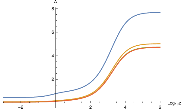
We see that varies modestly with redshift and with . As with late time values for should not to be taken too seriously for . The part of the plot that is most relevant to the loop distribution today for microlensing is large . The results are rather simple: and there is only about a factor of variation in as ranges from to near .
Appendix E Numbers of loops today in the universe as a whole
Loops formed at a given time will have size . As described previously, about 80% of the energy goes into loops with (radiation era) or (matter era) and about 20% goes into loops with . Set to describe the fraction of long string length that ends up in long loops. The comoving energy and the loop energy density is
| (E.1) |
where we have set . The velocity one scale model implies
| (E.2) |
and integrating in time
| (E.3) |
For short time increments this is
| (E.4) |
Large loops of a given size are made only at one instant so if we distinguish the loops of size then is nearly constant and
| (E.5) | |||||
| (E.6) |
Restoring “c” the birth rate density for loops of size born at time is
| (E.7) |
and the resultant density size distribution at time
| (E.8) | |||||
| (E.9) |
Integrating over and we have
| (E.10) | |||||
| (E.11) | |||||
| (E.12) |
where we require or . The quantity is a slowly varying function of time (on account of but we will treat the value as constant, taking typical numerical values at in the radiation era because the numerous small loops are of greatest observational interest. The form for peaks at but the quantity of interest for observational purposes is usually weighted by (or higher powers). The characteristic dissipative scale of the loop at the end of its life is . For a simple numerical estimate today when most loops are generated in the radiative era we write
| (E.13) | |||||
| (E.14) |
and using we have
| (E.15) |
The approximate expression suitable for describing the today’s loops formed in the radiative era, explicit numerical expressions for density of loops, the characteristic length and mass of the loops just evaporating, and the mass densities today are given in the main text.
It is also useful to have accurate descriptions of the loop distribution at earlier times. When the universe experiences pure power law expansion the loop distribution function at time is
| (E.16) |
During the radiation era () the result is identical to Eq.(4.14) except for the factor which accounts for the switch from radiation to matter expansion at . One derives , , , and for an observer at time .
Appendix F String Loop Clustering
Network simulations show that a loop cut of the network at time with length and has a moderately relativistic center of mass motion. The rms velocity . Smaller loops typically move faster than larger ones. The loop lives before shrinking to zero size. The characteristic number of e-foldings of the universe before the loop evaporates, , is large if . Cosmic superstrings can have very small tensions since is exponentially warped.
The universe’s expansion steadily damps any free particle’s peculiar motion. If a slow moving loop is at the right position when a perturbation begins to form then it can be captured. In the normal process of structure formation, cold dark matter is captured in precisely this manner.
Cold dark matter must be long-lived and, once accreted, is permanently bound to the nonlinear object ultimately formed. Superstring loops radiate energy steadily and their residence is temporary. The pattern of a loop’s emission is generally anisotropic, leading to a net recoil on the center of mass of the loop, the so-called “rocket effect.” When is less than a critical value the loop experiences the following sequence of events: (1) damped peculiar motion, (2) possible capture by growing gravitational perturbation, (3) residence in the bound object for a time comparable to , (4) ejection by the rocket effect towards the end of its life, (5) complete evaporation in the IGM. By contrast, when is too big the acceleration from the rocket effect occurs before capture. Such a loop never slows and evaporates in the IGM.
This process was studied in some detail in ref. [31]. An analytic estimate of the critical string tension for capture to radius in the Galaxy is
| (F.1) |
where is the initial loop velocity. The criterion leads to capture. This is a conservative estimate for clustering. It is based on assuming that the rocket effect is maximally effective in two senses. First, the orientation of the force on the center of mass of the loop is fixed. The loop receives the maximum cumulative impulse. The loop breaks free the gravitational potential at the earliest possible moment. Second, the magnitude of the rocket effect is estimated using loops with cusps. Studies of various loop configurations (with a few kinks or cusps) show that the cusps generate the greatest anisotropy in gravitational wave emission.
To check this understanding ref. [31] carried out a numerical calculation of how loops (born from a scaling string network) interact with a growing, galactic scale perturbation in cosmology. Initial conditions (loop sizes, velocities) were sampled and loop positions calculated. All the dynamical phases above were identified. The summary is simple: small tension loops of all sizes simply track the dark matter that collapses to form the bound object.
Let the enhancement of the dark matter within the Galaxy today with respect to the universe as a whole be
| (F.2) |
where and are spatially dependent. The simulation shows that the enhancement of the loops in the Galactic halo with respect to the universe as a whole, , is proportional to with proportionality constant that is primarily a function of tension:
| (F.3) |
If loops followed CDM perfectly then . In fact, for the Galactic halo
| (F.4) | |||||
| (F.5) | |||||
For the limiting enhancement is . In the limit we do not have because the rocket effect always removes the loop from the Galaxy before it fully evaporates.
At the local solar position we estimate so is a huge enhancement with respect to the universe as a whole for low tension strings.
Assume the anisotropy of the gravitational wave emission. As in the original study, this assumption minimizes the extent of clustering because it maximizes the effect of the rocket recoil and removes loops from the halo as soon as possible. The capture and ejection of the loops is the same for the joint axion and gravitational case as it is for the pure gravitational case with the substitution . The degree of clustering is set by the tension-dependent proportionality constant that becomes ; the spectrum is given by eq. 4.14.
Appendix G Galactic fit to the String Density
The dark matter halo of the galaxy is from Binney and Tremaine and fully described in Appendix J. One version is for a NFW-like cusp at the center and the other is for a core. We adopt a spherical version of the model . The dark matter enhancement is
| (G.1) |
the critical density (for km/s/Mpc) is
| (G.2) |
and the dark matter fraction is
| (G.3) |
Numerically, the spatially varying, dark matter enhancement is
| (G.4) |
The string enhancement is
| (G.5) |
and the spatially varying local string density as
| (G.6) |
and the bracket is the average for the loop density for the universe as a whole. Note that the string loop distribution, a function of , is enhanced by a single factor.
Appendix H Implementation for -CDM
Friedmann’s equation is
| (H.1) | |||||
| (H.2) | |||||
| (H.3) | |||||
| (H.4) |
with
| (H.5) | |||||
| (H.6) | |||||
| (H.7) | |||||
| (H.8) | |||||
| (H.9) |
And rewrite the terms in K’s equations by to give
| (H.11) | |||||
| (H.12) | |||||
| (H.13) |
The numerical results were pre-calculated for flat -CDM (, and ) and then used in the string network calculation. The quantity is shown in Fig. 15.

Appendix I Fit for the loop creation rate
The loop creation rate is written
| (I.1) |
where
| (I.2) |
The factor varies modestly. We use a simple Pade approximant for each factor and find
| (I.3) | |||||
| (I.4) | |||||
| (I.5) | |||||
| (I.6) | |||||
| (I.7) | |||||
| (I.8) |
and
| (I.9) | |||||
| (I.10) | |||||
| (I.11) |
This fit reproduces the numerical results to relative error and absolute error for .
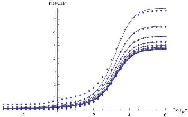
Appendix J Dark matter model
The dark matter halo of the galaxy is empirically described (Binney and Tremaine) by an ellipsoidal distribution; two models are given with parameters as follows:
| (J.1) | |||||
| (J.2) | |||||
| (J.3) | |||||
| (J.4) | |||||
| (J.5) | |||||
| (J.6) | |||||
| (J.7) |
where, has been set arbitrarily. We take so that the distribution is spherical. One model is for an NFW-like cusp and other is for a core.
Appendix K Lensing without light physically circling a string
A straight string in 3+1 dimensions generates a deficit angle in a plane perpendicular to it. There exist two straight line paths for light from a point source to an observer on the opposite side of the string in the same plane if they are all aligned, via circumnavigating the string in opposite senses, thus producing a double image.
In the braneworld scenario, although both the source (e.g., a star) and the observer are inside the standard model branes in “the standard model” throat, there are cosmic superstrings in other warped throats, so photons can never physically circle around them. Here we analyze lensing in that situation. Lensing is a gravitational effect which is transmitted through the bulk spacetime so the effect is not unexpected.
K.1 Lensing in Minkowski-like spacetime
Let the background metric be Minkowski – in other words, choose scaled coordinates so that the warp factors are absorbed. Einstein’s equations in N spacetime dimensions are
| (K.1) |
where Greek indices range from to . For ordinary spacetime , and and we will retain as the 4-dimensional Newton’s constant. For we write where is a length scale and retain units for tension . Taking the trace, solving for in terms of , we recast the Einstein equations as
| (K.2) |
Next we linearize the metric about N-dimensional Minkowski
| (K.3) |
where is the small quantity and find
| (K.4) |
(with summation over from to ) and adopt the gauge to find
| (K.5) |
where we have taken to be first order.
Let the string lie along axis . Since the background metric is flat and has been scaled to Minkowski we can be agnostic as to whether is in the Standard model brane or not.
The stress energy tensor is
| (K.6) |
where is the delta function in coordinate direction i. The first and last elements correspond to and . The stress energy combination
| (K.7) |
and the first order set of equations is
| (K.8) |
We restrict to time-independent solutions with for to . The equations for the off-diagonal elements of vanish, so if the off-diagonal elements vanish at infinity they vanish everywhere. We restrict to solutions that are independent of the coordinate along the string (labeled by ), the perturbed metric elements are functions of the form and we drop the derivatives with respect to . Define the dimensional Laplacian: . We have
| (K.9) |
and for to
| (K.10) |
All these equations are of the form
| (K.11) |
The equation describes the potential of a point particle of mass in dimensions where is the area of k-sphere (, ; in general, ). If () then the mass is ().
Explicitly, the constants are
| (K.12) |
and
| (K.13) |
For normal spacetime, we have , so that and for the two dimensions perpendicular to axis we have
| (K.14) |
where represents the constant of integration since it’s not possible to set at infinity.
For integer we have (restoring an explicit c)
| (K.15) | |||||
| (K.16) |
and and .
For example, for , and we have
| (K.17) |
and
| (K.18) |
Now we consider the geodesic equation for the photon. The string lies in direction . Let the photon move in direction for the unperturbed Minkowski metric, . The coordinates for give the transverse separation from the string which lies along direction .
We seek the effect of the gravitational perturbation on the photon’s path. For the transverse directions the geodesic equation is
| (K.19) |
and to lowest order (for the unperturbed motion)
| (K.20) |
and we have
| (K.21) |
| (K.22) |
with other terms vanishing. So
| (K.23) |
With , we have
| (K.24) |
K.2 3+1 spacetime
Now we will be explicit for the case of non-compact spacetime with : the photon moves in the direction , the string lies along and there is one transverse dimensions . The string passes through . The photon separation from the string is and the unperturbed photon path is , so . The transverse change in velocity of the photon is
| (K.25) |
We need the results for
| (K.26) |
which gives
| (K.27) |
The integral over all gives
| (K.28) | |||||
| (K.29) |
where is the sign of . To lowest order, this is the angle of bending of the massless particle
| (K.30) |
This illustrates the usual bending angle in 4 spacetime dimensions where is the macroscopic dimension perpendicular to the line of sight and the string. The alignment of string, source and observer varies in the macroscopic dimension because all three elements are typically moving in the macroscopic dimensions. In string lensing the sign of switches, i.e. the photon circumnavigates the string in two distinct paths because of the variation of the macroscopic geometry. The two paths have different bending angles. When both paths are accessible the observer sees two images of the source.
K.3 non-compact spacetime
For we have . Here we carry out the calculation for the non-compact dimensional space.
We will be explicit for : the photon moves in the direction , the string lies along and there are transverse dimensions, is macroscopic and the rest are microscopic. Label ; for we will set to zero. The string passes through and (and the remaining microscopic dimensions are zero). The Standard model brane has (and the remaining microscopic dimensions are zero) and the photon is confined to the brane. The photon separation from the string is and the unperturbed photon path is , so .
From the previous calculations, we have
| (K.31) | |||||
| (K.32) |
which gives
| (K.33) |
The velocity impulse in the y direction is
| (K.34) |
where the integral
| (K.35) |
(for ). The net result is
| (K.36) |
The bending angle therefore depends upon the impact parameter measured with respect to the physical scale that was introduced at the beginning and that relates to .
Set , the scale of the maximum separation in the small dimensions transverse to the brane of the standard model. As the motion in the macroscopic dimensions sends , changing the sign of we have, asymptotically,
| (K.37) |
If one assumes that the minimal scale for then one infers an angular bending at that scale is qualitatively similar but quantitatively different than the case . Note however that these results depend, in general, upon unlike those in eqn. K.29.
K.4 compact spacetime
Here, we consider normal spacetime having one extra microscopic toroidal coordinate: , , . The photon moves in the direction , the string lies along , the macroscopic transverse dimension is and the microscopic, periodic transverse dimension is with length . The string passes through and where and the Standard model brane has (“s” for source and “f” for field point).
The equations of motion for the non-compact spacetime were
| (K.38) |
We now impose is periodic in but there is a subtlety. If we require that vanishes at large macroscopic distances then the -integral of the source on the right hand side must vanish just as the volume integral of stress-energy sources in general relativity must vanish for a closed manifold. In string theory constructions with orientifolds there is a source of stable negative energy density in the macroscopic dimensions, namely, the rigid negative tension orientifold planes. Because the volume of the macroscopic dimensions is so large compared to that of the compact dimensions only a very small negative energy density is actually needed. We expect the orientifold contribution cancels that of the strings in the microscopic dimension.
We will first construct a “jellium” like solution in which a local source of negative tension in the compact dimensions exactly balances that of the positive string contribution. We will show that the metric perturbations are finite and that the individual lensing contributions from positive and negative terms exactly cancel. Then we argue that the orientifold shifts the boundary conditions at infinity so that we can simultaneously turn on the orientifold contribution and turn off the smooth jellium term. For photons moving in the Standard model brane we recover the exact 3+1 result for lensing by a string in a hidden throat.
The periodic solution may be constructed from the non-compact solution with two steps. First, adding image strings at positions for integer with . Second, by including a local homogeneous contribution (the jellium) that cancels the string component for each image:
The schematic form for one string () in the non-compact solution is
| (K.39) | |||||
| (K.40) | |||||
| (K.41) | |||||
| (K.42) |
with . Here, is the macroscopic distance from the field point to the string.
The schematic form for the background contribution for one string ()
| (K.43) | |||||
| (K.44) | |||||
| (K.45) |
Since the equations are linear we add the solutions for each discrete image and also the contribution of strings of negative tension uniformly distributed in the compact dimension (tension per compact length ). The individual sums are not absolutely convergent but the series with paired positive and negative contributions of each image grouped together is. Large contributions are small and convergent.
The total result summed over all images is
| (K.46) | |||||
Taking the derivative with respect , integrating over the photon path gives
| (K.50) | |||||
| (K.51) | |||||
| (K.52) | |||||
| (K.53) |
For the term simplifies to
| (K.54) |
and the sum in telescopes and successive terms cancel. Examining the representation for large but finite with and gives
| (K.55) | |||||
| (K.56) |
Since this result is independent of and , the final result is
| (K.57) |
This cancellation is not surprising since the net energy density is zero by construction.
The angle change for for the two terms are
| (K.58) |
The size of the jellium term is
| (K.59) | |||||
| (K.60) | |||||
| (K.61) |
Now, we argue that we can alter the boundary condition at large macroscopic distances replacing the jellium contribution with that of a properly chosen orientifold contribution. We are left with only the string lensing. If we take then this is identical to the result in normal spacetime.
References
- [1] T. W. B. Kibble, “Topology of Cosmic Domains and Strings,” J. Phys. A 9, 1387 (1976).
- [2] A. Villenkin and E.P.S. Shellard, Cosmic strings and other topological defects, Cambridge University Press, 2000.
- [3] L. Sousa and P. P. Avelino, Phys. Rev. D 94, no. 6, 063529 (2016) [arXiv:1606.05585 [astro-ph.CO]].
- [4] J. J. Blanco-Pillado and K. D. Olum, “Stochastic gravitational wave background from smoothed cosmic string loops,” arXiv:1709.02693 [astro-ph.CO].
- [5] J. J. Blanco-Pillado, K. D. Olum and X. Siemens, “New limits on cosmic strings from gravitational wave observation,” arXiv:1709.02434 [astro-ph.CO].
- [6] D. Baumann and L. McAllister, “Inflation and String Theory,” arXiv:1404.2601 [hep-th].
- [7] N. T. Jones, H. Stoica and S.-H. H. Tye, “Brane interaction as the origin of inflation,” JHEP 0207, 051 (2002) [hep-th/0203163].
- [8] S. Sarangi and S.-H. H. Tye, “Cosmic string production towards the end of brane inflation,” Phys. Lett. B 536, 185 (2002), [hep-th/0204074].
- [9] N. T. Jones, H. Stoica and S.-H. H. Tye, “The Production, spectrum and evolution of cosmic strings in brane inflation,” Phys. Lett. B 563, 6 (2003) [hep-th/0303269].
- [10] E. J. Copeland, R. C. Myers and J. Polchinski, “Cosmic F- and D-strings,” JHEP 0406, 013 (2004), hep-th/0312067.
- [11] B. P. Abbott et al. “Observation of Gravitational Waves from a Binary Black Hole Merger,” Phys. Rev. Lett. 116, 061102 (2016).
- [12] T. Damour and A. Vilenkin, “Gravitational radiation from cosmic (super)strings: Bursts, stochastic background, and observational windows,” Phys. Rev. D 71, 063510 (2005) [hep-th/0410222].
- [13] T. Damour and A. Vilenkin, “Gravitational wave bursts from cusps and kinks on cosmic strings,” Phys. Rev. D 64, 064008 (2001) [gr-qc/0104026].
- [14] D. F. Chernoff and S.-H. H. Tye, “Cosmic String Detection via Microlensing of Stars,” arXiv:0709.1139 [astro-ph].
- [15] D. F. Chernoff and S.-H. H. Tye, “Inflation, string theory and cosmic strings,” Int. J. Mod. Phys. D 24, no. 03, 1530010 (2015) [arXiv:1412.0579 [astro-ph.CO]].
- [16] S. B. Giddings, S. Kachru and J. Polchinski, “Hierarchies from fluxes in string compactifications,” Phys. Rev. D 66, 106006 (2002), hep-th/0105097.
- [17] S. Kachru, R. Kallosh, A. Linde and S. P. Trivedi, “De Sitter vacua in string theory”, Phys. Rev. D 68, 046005 (2003), hep-th/0301240.
- [18] J. Polchinski, “Dirichlet Branes and Ramond-Ramond charges,” Phys. Rev. Lett. 75, 4724 (1995) [hep-th/9510017].
- [19] G. R. Dvali and S.-H. H. Tye, “Brane inflation,” Phys. Lett. B 450, 72 (1999), hep-ph/9812483.
- [20] G. R. Dvali, Q. Shafi and S. Solganik, “D-brane inflation,” hep-th/0105203.
- [21] C. P. Burgess, M. Majumdar, D. Nolte, F. Quevedo, G. Rajesh and R. J. Zhang, “The Inflationary brane anti-brane universe,” JHEP 0107, 047 (2001) [hep-th/0105204].
- [22] S. Kachru, R. Kallosh, A. Linde, J. Maldacena, L. McAllister and S. P. Trivedi, “Towards inflation in string theory,” JCAP 0310 (2003) 013, hep-th/0308055.
- [23] Planck Collaboration, arXiv : 1303.5082 [astro-ph.co].
- [24] H. Firouzjahi and S.-H. H. Tye, “Brane inflation and cosmic string tension in superstring theory,” JCAP 0503, 009 (2005) [hep-th/0501099].
- [25] R. Bean, S. E. Shandera, S.-H. H. Tye and J. Xu, “Comparing brane inflation to WMAP,” JCAP 0705, 004 (2007) [hep-th/0702107].
- [26] L. Kofman and P. Yi, “Reheating the universe after string theory inflation,” Phys. Rev. D 72, 106001 (2005) [hep-th/0507257].
- [27] X. Chen and S.-H. H. Tye, “Heating in brane inflation and hidden dark matter,” JCAP 0606, 011 (2006) [hep-th/0602136].
- [28] D. Chialva, G. Shiu and B. Underwood, “Warped reheating in multi-throat brane inflation,” JHEP 0601, 014 (2006), hep-th/0508229.
- [29] M. G. Jackson, N. T. Jones and J. Polchinski, “Collisions of cosmic F- and D-strings,” JHEP 0510, 013 (2005), hep-th/0405229.
- [30] A. Avgoustidis and E. P. S. Shellard, “Effect of reconnection probability on cosmic (super)string network density,” Phys. Rev. D 73, 041301 (2006) [astro-ph/0512582].
- [31] D. F. Chernoff, “Clustering of Superstring Loops,” arXiv:0908.4077 [astro-ph.CO].
- [32] A. Avgoustidis and E. P. S. Shellard, “Cosmic string evolution in higher dimensions,” Phys. Rev. D 71, 123513 (2005) [hep-ph/0410349].
- [33] M. Sakellariadou, “A Note on the evolution of cosmic string/superstring networks,” JCAP 0504, 003 (2005) [hep-th/0410234].
- [34] H. Firouzjahi, L. Leblond and S.-H. H. Tye, “The (p,q) string tension in a warped deformed conifold,” JHEP 0605, 047 (2006) [hep-th/0603161].
- [35] S.S. Gubser, C. Herzog and I.R. Klebanov, ”Symmetry breaking and axionic strings in the warped deformed conifold”, JHEP 09 (2004) 036, hep-th/0405282.
- [36] X. Siemens, X. Martin and K. D. Olum, “Dynamics of Cosmic Necklaces,” Nucl. Phys. B 595, 402 (2001), astro-ph/0005411.
- [37] L. Leblond, B. Shlaer and X. Siemens, “Gravitational Waves from Broken Cosmic Strings: The Bursts and the Beads,” Phys. Rev. D 79, 123519 (2009) [arXiv:0903.4686 [astro-ph.CO]].
- [38] L. Leblond and S.-H. H. Tye, “Stability of D1 strings inside a D3-brane,” JHEP 0403, 055 (2004) [hep-th/0402072].
- [39] H. Firouzjahi, “Energy radiation by cosmic superstrings in brane inflation,” Phys. Rev. D 77, 023532 (2008) [arXiv:0710.4609 [hep-th]].
- [40] R. Gwyn, M. Sakellariadou and S. Sypsas, “Theoretical constraints on brane inflation and cosmic superstring radiation,” JHEP 1109, 075 (2011) [arXiv:1105.1784 [hep-th]].
- [41] A. Avgoustidis, “Cosmic String Dynamics and Evolution in Warped Spacetime,” Phys. Rev. D 78, 023501 (2008) [arXiv:0712.3224 [hep-th]].
- [42] A. Avgoustidis, S. Chadburn and R. Gregory, “Cosmic superstring trajectories in warped compactifications,” Phys. Rev. D 86, 063516 (2012) [arXiv:1204.0973 [hep-th]].
- [43] M. R. DePies and C. J. Hogan, “Stochastic Gravitational Wave Background from Light Cosmic Strings,” Phys. Rev. D 75, 125006 (2007) [astro-ph/0702335].
- [44] S. Kuroyanagi, K. Miyamoto, T. Sekiguchi, K. Takahashi and J. Silk, “Forecast constraints on cosmic string parameters from gravitational wave direct detection experiments,” Phys. Rev. D 86, 023503 (2012) [arXiv:1202.3032 [astro-ph.CO]].
- [45] S. Kuroyanagi, K. Miyamoto, T. Sekiguchi, K. Takahashi and J. Silk, “Forecast constraints on cosmic strings from future CMB, pulsar timing and gravitational wave direct detection experiments,” Phys. Rev. D 87, no. 2, 023522 (2013) Erratum: [Phys. Rev. D 87, no. 6, 069903 (2013)] [arXiv:1210.2829 [astro-ph.CO]].
- [46] J. J. Blanco-Pillado, K. D. Olum and B. Shlaer, “The number of cosmic string loops,” Phys. Rev. D 89, no. 2, 023512 (2014) [arXiv:1309.6637 [astro-ph.CO]].
- [47] M. R. DePies and C. J. Hogan, “Harmonic Gravitational Wave Spectra of Cosmic String Loops in the Galaxy,” arXiv:0904.1052 [astro-ph.CO].
- [48] J. P. Uzan and F. Bernardeau, “Cosmic strings lens phenomenology: General properties of distortion fields,” Phys. Rev. D 63, 023004 (2001) [astro-ph/0004105].
- [49] E. Witten, “Cosmic Superstrings,” Phys. Lett. 153B, 243 (1985).
- [50] S. Sarangi and S.-H. H. Tye, “Interbrane potential and the decay of a nonBPS D-brane to closed strings,” Phys. Lett. B 573, 181 (2003) [hep-th/0307078].
- [51] J. H. Schwarz, “An SL(2,Z) multiplet of type IIB superstrings,” Phys. Lett. B 360, 13 (1995) [Erratum-ibid. B 364, 252 (1995)], hep-th/9508143.
- [52] A. Avgoustidis, A. Pourtsidou and M. Sakellariadou, “Zipping and Unzipping in String Networks: Dynamics of Y-junctions,” Phys. Rev. D 91, no. 2, 025022 (2015) [arXiv:1411.7959 [hep-th]].
- [53] S.-H. H. Tye, I. Wasserman and M. Wyman, “Scaling of multi-tension cosmic superstring networks,” Phys. Rev. D 71, 103508 (2005) Erratum: [Phys. Rev. D 71, 129906 (2005)] [astro-ph/0503506].
- [54] I. R. Klebanov and M. J. Strassler, “Supergravity and a confining gauge theory: Duality cascades and chi-SB-resolution of naked singularities,” JHEP 0008, 052 (2000), hep-th/0007191.
- [55] S. Shandera, B. Shlaer, H. Stoica and S.-H. H. Tye, “Interbrane interactions in compact spaces and brane inflation,” JCAP 0402, 013 (2004) [hep-th/0311207].
- [56] S. E. Shandera and S.-H. H. Tye, “Observing brane inflation,” JCAP 0605, 007 (2006) [hep-th/0601099].
- [57] R. C. Myers, “Dielectric branes,” JHEP 9912, 022 (1999) [hep-th/9910053].
- [58] N. T. Jones and S. H. H. Tye, “An Improved brane anti-brane action from boundary superstring field theory and multivortex solutions,” JHEP 0301, 012 (2003) [hep-th/0211180].
- [59] B. Shlaer and M. Wyman, “Cosmic superstring gravitational lensing phenomena: Predictions for networks of (p,q) strings,” Phys. Rev. D 72, 123504 (2005), hep-th/0509177.
- [60] P. Candelas, A. Font, S. H. Katz and D. R. Morrison, “Mirror symmetry for two parameter models. 2.,” Nucl. Phys. B 429, 626 (1994), hep-th/9403187.
- [61] S. Kachru, J. Pearson and H. L. Verlinde, “Brane / flux annihilation and the string dual of a nonsupersymmetric field theory,” JHEP 0206 (2002) 021 [hep-th/0112197].
- [62] W. Hu, R. Barkana and A. Gruzinov, “Cold and fuzzy dark matter,” Phys. Rev. Lett. 85, 1158 (2000) [astro-ph/0003365].
- [63] L. Hui, J. P. Ostriker, S. Tremaine and E. Witten, Phys. Rev. D 95, no. 4, 043541 (2017) doi:10.1103/PhysRevD.95.043541 [arXiv:1610.08297 [astro-ph.CO]].
- [64] M. Hindmarsh, K. Rummukainen and D. J. Weir, “Numerical simulations of necklaces in SU(2) gauge-Higgs field theory,” Phys. Rev. D 95, no. 6, 063520 (2017) [arXiv:1611.08456 [astro-ph.CO]].
- [65] D. R. Lorimer, M. Bailes, M. A. McLaughlin, D. J. Narkevic and F. Crawford, “A bright millisecond radio burst of extragalactic origin,” Science 318, 777 (2007) doi:10.1126/science.1147532 [arXiv:0709.4301 [astro-ph]].
- [66] D. Thornton et al., “A Population of Fast Radio Bursts at Cosmological Distances,” Science 341, no. 6141, 53 (2013) doi:10.1126/science.1236789 [arXiv:1307.1628 [astro-ph.HE]].
- [67] T. Vachaspati, “Cosmic Sparks from Superconducting Strings,” Phys. Rev. Lett. 101, 141301 (2008) [arXiv:0802.0711 [astro-ph]].
- [68] Y. F. Cai, E. Sabancilar and T. Vachaspati, “Radio bursts from superconducting strings,” Phys. Rev. D 85, 023530 (2012) [arXiv:1110.1631 [astro-ph.CO]].
- [69] L. V. Zadorozhna and B. I. Hnatyk, “Electromagnetic emission bursts from the near-cusp regions of superconducting cosmic strings,” Ukr. J. Phys. 54, 1149 (2009).
- [70] Y. F. Cai, E. Sabancilar, D. A. Steer and T. Vachaspati, “Radio Broadcasts from Superconducting Strings,” Phys. Rev. D 86, 043521 (2012) doi:10.1103/PhysRevD.86.043521 [arXiv:1205.3170 [astro-ph.CO]].
- [71] Y. W. Yu, K. S. Cheng, G. Shiu and S.-H. H. Tye, “Implications of fast radio bursts for superconducting cosmic strings,” JCAP 1411, no. 11, 040 (2014) doi:10.1088/1475-7516/2014/11/040 [arXiv:1409.5516 [astro-ph.HE]].
- [72] J. Ye, K. Wang and Y. F. Cai, “Superconducting Cosmic Strings as Sources of Cosmological Fast Radio Bursts,” arXiv:1705.10956 [astro-ph.HE].
- [73] V. Berezinsky, B. Hnatyk and A. Vilenkin, “Gamma-ray bursts from superconducting cosmic strings,” Phys. Rev. D 64, 043004 (2001) [astro-ph/0102366].
- [74] A. Gruzinov and A. Vilenkin, “Fireballs from Superconducting Cosmic Strings,” JCAP 1701, no. 01, 029 (2017) [arXiv:1608.05396 [astro-ph.HE]].
- [75] R. Brandenberger, B. Cyr and A. V. Iyer, “Fast Radio Bursts from the Decay of Cosmic String Cusps,” arXiv:1707.02397 [astro-ph.CO].
- [76] J. K. Bloomfield and D. F. Chernoff, “Cosmic String Loop Microlensing,” Phys. Rev. D 89, no. 12, 124003 (2014) doi:10.1103/PhysRevD.89.124003 [arXiv:1311.7132 [astro-ph.CO]].
- [77] T. W. B. Kibble, “Evolution of a system of cosmic strings,” Nucl. Phys. B 252, 227 (1985) Erratum: [Nucl. Phys. B 261, 750 (1985)].
- [78] D. P. Bennett and F. R. Bouchet, “Evidence for a Scaling Solution in Cosmic String Evolution,” Phys. Rev. Lett. 60, 257 (1988).
- [79] D. P. Bennett and F. R. Bouchet, “Cosmic string evolution,” Phys. Rev. Lett. 63, 2776 (1989).
- [80] D. P. Bennett and F. R. Bouchet, “High Resolution Simulations Of Cosmic String Evolution: Part 1. Numerics And Long String Evolution. Part 2. Small Scale Structure And Loops,” PUPT-90-1162.
- [81] B. Allen and E. P. S. Shellard, “Cosmic string evolution: a numerical simulation,” Phys. Rev. Lett. 64, 119 (1990).
- [82] A. Albrecht and N. Turok, “Evolution of Cosmic Strings,” Phys. Rev. Lett. 54, 1868 (1985).
- [83] A. Albrecht and N. Turok, “Evolution of Cosmic String Networks,” Phys. Rev. D 40, 973 (1989).
- [84] D. Austin, E. J. Copeland and T. W. B. Kibble, “Evolution of cosmic string configurations,” Phys. Rev. D 48, 5594 (1993) [hep-ph/9307325].
- [85] J. Polchinski and J. V. Rocha, “Analytic study of small scale structure on cosmic strings,” Phys. Rev. D 74, 083504 (2006) [hep-ph/0606205].
- [86] F. Dubath, J. Polchinski and J. V. Rocha, “Cosmic String Loops, Large and Small,” Phys. Rev. D 77, 123528 (2008) [arXiv:0711.0994 [astro-ph]].
- [87] J. Polchinski and J. V. Rocha, “Cosmic string structure at the gravitational radiation scale,” Phys. Rev. D 75, 123503 (2007) [gr-qc/0702055 [GR-QC]].
- [88] J. Polchinski, “Cosmic String Loops and Gravitational Radiation,” arXiv:0707.0888 [astro-ph].
- [89] C. J. A. P. Martins and E. P. S. Shellard, “Fractal properties and small-scale structure of cosmic string networks,” Phys. Rev. D 73, 043515 (2006) [astro-ph/0511792].
- [90] C. Ringeval, M. Sakellariadou and F. Bouchet, “Cosmological evolution of cosmic string loops,” JCAP 0702, 023 (2007) [astro-ph/0511646].
- [91] K. D. Olum and V. Vanchurin, “Cosmic string loops in the expanding Universe,” Phys. Rev. D 75, 063521 (2007) [astro-ph/0610419].
- [92] V. Vanchurin, K. D. Olum and A. Vilenkin, “Scaling of cosmic string loops,” Phys. Rev. D 74, 063527 (2006) [gr-qc/0511159].
- [93] J. J. Blanco-Pillado, K. D. Olum and B. Shlaer, “A new parallel simulation technique,” J. Comput. Phys. 231, 98 (2012) [arXiv:1011.4046 [physics.comp-ph]].
- [94] J. J. Blanco-Pillado, K. D. Olum and B. Shlaer, “Large parallel cosmic string simulations: New results on loop production,” Phys. Rev. D 83, 083514 (2011) [arXiv:1101.5173 [astro-ph.CO]].
- [95] D. P. Bennett, “The evolution of cosmic strings,” Phys. Rev. D 33, 872 (1986) Erratum: [Phys. Rev. D 34, 3932 (1986)].
- [96] D. P. Bennett, “Evolution of cosmic strings. 2.,” Phys. Rev. D 34, 3592 (1986).
- [97] C. J. A. P. Martins and E. P. S. Shellard, “Extending the velocity dependent one scale string evolution model,” Phys. Rev. D 65, 043514 (2002) [hep-ph/0003298].
- [98] L. Pogosian and T. Vachaspati, “Cosmic microwave background anisotropy from wiggly strings,” Phys. Rev. D 60, 083504 (1999) [astro-ph/9903361].
- [99] R. A. Battye, J. Robinson and A. Albrecht, “Structure formation by cosmic strings with a cosmological constant,” Phys. Rev. Lett. 80, 4847 (1998) [astro-ph/9711336].
- [100] C. J. A. P. Martins and E. P. S. Shellard, “String evolution with friction,” Phys. Rev. D 53, 575 (1996) [hep-ph/9507335].
- [101] J. Aasi et al. [LIGO Scientific Collaboration], “Advanced LIGO,” Class. Quant. Grav. 32, 074001 (2015) [arXiv:1411.4547 [gr-qc]].
- [102] T. Accadia et al., “Status of the Virgo project,” Class. Quant. Grav. 28, 114002 (2011).
- [103] Y. Aso et al. [KAGRA Collaboration], “Interferometer design of the KAGRA gravitational wave detector,” Phys. Rev. D 88, no. 4, 043007 (2013) [arXiv:1306.6747 [gr-qc]].
- [104] M. Evans [LIGO Scientific and VIRGO and KAGRA Collaborations], “Gravitational wave detection with advanced ground based detectors,” Gen. Rel. Grav. 46, no. 10, 1778 (2014).
- [105] H. Audley et al., “Laser Interferometer Space Antenna,” arXiv:1702.00786 [astro-ph.IM].
- [106] S. Kawamura et al., “The Japanese space gravitational wave antenna: DECIGO,” Class. Quant. Grav. 28, 094011 (2011).
- [107] Z. Arzoumanian et al. [NANOGrav Collaboration], “The NANOGrav Nine-year Data Set: Limits on the Isotropic Stochastic Gravitational Wave Background,” Astrophys. J. 821, no. 1, 13 (2016) [arXiv:1508.03024 [astro-ph.GA]].
- [108] L. Lentati et al., “European Pulsar Timing Array Limits On An Isotropic Stochastic Gravitational-Wave Background,” Mon. Not. Roy. Astron. Soc. 453, no. 3, 2576 (2015) [arXiv:1504.03692 [astro-ph.CO]].
- [109] G. Hobbs, “The Parkes Pulsar Timing Array,” Class. Quant. Grav. 30, 224007 (2013) [arXiv:1307.2629 [astro-ph.IM]].
- [110] T. Damour and A. Vilenkin, “Gravitational wave bursts from cosmic strings,” Phys. Rev. Lett. 85, 3761 (2000) [gr-qc/0004075].
- [111] X. Siemens, V. Mandic and J. Creighton, “Gravitational wave stochastic background from cosmic (super)strings,” Phys. Rev. Lett. 98, 111101 (2007) [astro-ph/0610920].
- [112] B. P. Abbott et al. [LIGO Scientific and Virgo Collaborations], “Constraints on cosmic strings using data from the first Advanced LIGO observing run,” arXiv:1712.01168 [gr-qc].
- [113] L. Lorenz, C. Ringeval and M. Sakellariadou, JCAP 1010, 003 (2010) doi:10.1088/1475-7516/2010/10/003 [arXiv:1006.0931 [astro-ph.CO]].
- [114] C. Ringeval and T. Suyama, JCAP 1712, no. 12, 027 (2017) doi:10.1088/1475-7516/2017/12/027 [arXiv:1709.03845 [astro-ph.CO]].
- [115] C. S. Unnikrishnan, “IndIGO and LIGO-India: Scope and plans for gravitational wave research and precision metrology in India,” Int. J. Mod. Phys. D 22, 1341010 (2013) [arXiv:1510.06059 [physics.ins-det]].