\coltauthor

INRIA - Département d’Informatique de l’ENS
Ecole Normale Supérieure, CNRS, INRIA, PSL Research University

Exponential Convergence of Testing Error
for Stochastic Gradient Methods

Loucas Pillaud-Vivien Email: loucas.pillaud-vivien@inria.fr Alessandro Rudi Email: alessandro.rudi@inria.fr Francis Bach Email: francis.bach@inria.fr Affiliation:

Abstract

We consider binary classification problems with positive definite kernels and square loss, and study the convergence rates of stochastic gradient methods. We show that while the excess testing loss (squared loss) converges slowly to zero as the number of observations (and thus iterations) goes to infinity, the testing error (classification error) converges exponentially fast if low-noise conditions are assumed. To achieve these rates of convergence we show sharper high-probability bounds with respect to the number of observations for stochastic gradient descent.

keywords

SGD, positive-definite kernels, margin condition, binary classification.

1 Introduction

Stochastic gradient methods are now ubiquitous in machine learning, both from the practical side, as a simple algorithm that can learn from a single or a few passes over the data (Bottou and Le Cun, 2005), and from the theoretical side, as it leads to optimal rates for estimation problems in a variety of situations (Nemirovski and Yudin, 1983; Polyak and Juditsky, 1992).

They follow a simple principle (Robbins and Monro, 1951): to find a minimizer of a function $F$ defined on a vector space from noisy gradients, simply follow the negative stochastic gradient and the algorithm will converge to a stationary point, local minimum or global minimum of $F$ (depending on the properties of the function $F$ ), with a rate of convergence that decays with the number of gradient steps $n$ typically as $O(1/\sqrt{n})$ , or $O(1/n)$ depending on the assumptions which are made on the problem (Polyak and Juditsky, 1992; Nesterov and Vial, 2008; Nemirovski et al., 2009; Shalev-Shwartz et al., 2007; Xiao, 2010; Bach and Moulines, 2011; Bach and Moulines, 2013; Dieuleveut et al., 2017, see, e.g.,).

On the one hand, these rates are optimal for the estimation of the minimizer of a function given access to noisy gradients (Nemirovski and Yudin, 1983), which is essentially the usual machine learning set-up where the function $F$ is the expected loss, e.g., logistic or hinge for classification, or least-squares for regression, and the noisy gradients are obtained from sampling a single pair of observations.

On the other hand, although these rates as $O(1/\sqrt{n})$ or $O(1/n)$ are optimal, there are a variety of extra assumptions that allow for faster rates, even exponential rates.

First, for stochastic gradient from a finite pool, that is for $F=\frac{1}{k}\sum_{i=1}^{k}F_{i}$ , a sequence of works starting from SAG (Le Roux et al., 2012), SVRG (Johnson and Zhang, 2013), SAGA (Defazio et al., 2014), have shown explicit exponential convergence. However, these results, once applied to machine learning where the function $F_{i}$ is the loss function associated with the $i$ -th observation of a finite training data set of size $k$ , say nothing about the loss on unseen data (test loss). The rates we present in this paper are on unseen data.

Second, assuming that at the optimum all stochastic gradients are equal to zero, then for strongly-convex problems (e.g., linear predictions with low-correlated features), linear convergence rates can be obtained for test losses (Solodov, 1998; Schmidt and Le Roux, 2013). However, for supervised machine learning, this has limited relevance as having zero gradients for all stochastic gradients at the optimum essentially implies prediction problems with no uncertainty (that is, the output is a deterministic function of the input). Moreover, we can only get an exponential rate for strongly-convex problems and thus this imposes a parametric noiseless problem, which limits the applicability (even if the problem was noiseless, this can only reasonably be in a non-parametric way with neural networks or positive definite kernels). Our rates are on noisy problems and on infinite-dimensional problems where we can hope that we approach the optimal prediction function with large numbers of observations. For prediction functions described by a reproducing kernel Hilbert space, and for the square loss, the excess testing loss (equal to testing loss minus the minimal testing loss over all measurable prediction functions) is known to converge to zero at a subexponential rate typically greater than $O(1/n)$ (Dieuleveut and Bach, 2016; Dieuleveut et al., 2017), these rates being optimal for the estimation of testing losses.

Going back to the origins of supervised machine learning with binary labels, we will not consider getting to the optimal testing loss (using a convex surrogate such as logistic, hinge or least-squares) but the testing error (number of mistakes in predictions), also referred to as the 0-1 loss.

It is known that the excess testing error (testing error minus the minimal testing error over all measurable prediction functions) is upper bounded by a function of the excess testing loss (Zhang, 2004; Bartlett et al., 2006), but always with a loss in the convergence rate (e.g., no difference or taking square roots). Thus a slow rate in $O(1/n)$ or $O(1/\sqrt{n})$ on the excess loss leads to a slow(er) rate on the excess testing error.

Such general relationships between excess loss and excess error have been refined with the use of margin conditions, which characterize how hard the prediction problems are (Mammen and Tsybakov, 1999, see, e.g.,). Simplest input points are points where the label is deterministic (i.e., conditional probabilities of the label are equal to zero or one), while hardest points are the ones where the conditional probabilities are equal to $1/2$ . Margin conditions quantify the mass of input points which are hardest to predict, and lead to improved transfer functions from testing losses to testing errors, but still no exponential convergence rates (Bartlett et al., 2006).

In this paper, we consider the strongest margin condition, that is conditional probabilities are bounded away from $1/2$ , but not necessarily equal to $0$ or $1$ . This assumption on the learning problem has been used in the past to show that regularized empirical (convex) risk minimization leads to exponential convergence rates (Audibert and Tsybakov, 2007; Koltchinskii and Beznosova, 2005). Our main contribution is to show that stochastic gradient descent also achieves similar rates (see an empirical illustration in Figure 2 in the Appendix A). This requires several side contributions that are interesting on their own, that is, a new and simple formalization of the learning problem that allows exponential rates of estimation (regardless of the algorithms used to find the estimator) and a new concentration result for averaged stochastic gradient descent (SGD) applied to least-squares, which is finer than existing work (Bach and Moulines, 2013).

The paper is organized as follows: in Section 2, we present the learning set-up, namely binary classification with positive definite kernels, with a particular focus on the relationship between errors and losses. Our main results rely on a generic condition for which we give concrete examples in Section 3. In Section 4, we present our version of stochastic gradient descent, with the use of tail averaging (Jain et al., 2016), and provide new deviation inequalities, which we apply in Section 5 to our learning problem, leading to exponential convergence rates for the testing errors. We conclude in Section 6 by providing several avenues for future work. Finally, synthetic experiments illustrating our results can be found in Section A of the Appendix.

Main contributions of the paper.

We would like to underline that our main contributions are in the two following results; (a) we show in Theorem 10 the exponential convergence of stochastic gradient descent on the testing error, and (b) this result strongly rests on a new deviation inequality stated in Corollary 8 for stochastic gradient descent for least-square problems. This last result is interesting on its own and gives an improved high-probability result which does not depend on the dimension of the problem and has a tighter dependence on the strongly convex parameter –through the effective dimension of the problem, see Caponnetto and De Vito (2007); Dieuleveut and Bach (2016).

2 Problem Set-up

In this section, we present the general machine learning set-up, from generic assumptions to more specific assumptions.

2.1 Generic assumptions

We consider a measurable set ${\mathcal{X}}$ and a probability distribution $\rho$ on data $(x,y)\in{\mathcal{X}}\times\{-1,1\}$ ; we denote by ${\rho_{{\mathcal{X}}}}$ the marginal probability on $x$ , and by $\rho(\pm 1|x)$ the conditional probability that $y=\pm 1$ given $x$ . We have ${\mathbb{E}}(y|x)=\rho(1|x)-\rho(-1|x)$ . Our main margin condition is the following (and independent of the learning framework):

(A ) 1.

$|{\mathbb{E}}(y|x)|\geqslant\delta$ almost surely for some $\delta\in(0,1]$ .

This margin condition (often referred to as a low-noise condition) is commonly used in the theoretical study of binary classification (Mammen and Tsybakov, 1999; Audibert and Tsybakov, 2007; Koltchinskii and Beznosova, 2005), and usually takes the following form: $\forall\delta>0,\ {\mathbb{P}}(|{\mathbb{E}}(y|x)|<\delta)=O(\delta^{\alpha})$ for $\alpha>0$ . Here, however, $\delta$ is a fixed constant. Our stronger margin condition (A1) is necessary to show exponential convergence rates but we give also explicit rates in the case of the latter low-noise condition. This extension is derived in Appendix J and more precisely in Corollary 28. Note that the smaller the $\alpha$ , the larger the mass of inputs with hard-to-predict labels. Our condition corresponds to $\alpha=+\infty$ , and simply states that for all inputs, the problem is never totally ambiguous, and the degree of non-ambiguity is bounded from below by $\delta$ . When $\delta=1$ , then the label $y\in\{-1,1\}$ is a deterministic function of $x$ , but our results apply for all $\delta\in(0,1]$ and thus to noisy problems (with low noise). Note that problems like image classification or object recognition are well characterized by (A1). Indeed, the noise in classifying an image between two disparate classes (cars/pedestrians, bikes/airplanes) is usually way smaller that $1/2$ .

We will consider learning functions in a reproducing kernel Hilbert space (RKHS) ${\mathcal{H}}$ with kernel function $K:{\mathcal{X}}\times{\mathcal{X}}\to\mathbb{R}$ and dot-product $\langle\cdot,\cdot\rangle_{\mathcal{H}}$ . We make the following standard assumptions on ${\mathcal{H}}$ :

(A ) 2.

${\mathcal{H}}$ is a separable Hilbert space and there exists $R>0$ , such that for all $x\in{\mathcal{X}}$ , $K(x,x)\leqslant R^{2}$ .

For $x\in{\mathcal{X}}$ , we consider the function $K_{x}:{\mathcal{X}}\to\mathbb{R}$ defined as $K_{x}(x^{\prime})=K(x,x^{\prime})$ . We have the classical reproducing property for $g\in{\mathcal{H}}$ , $g(x)=\langle g,K_{x}\rangle_{\mathcal{H}}$ (Shawe-Taylor and Cristianini, 2004; Schölkopf and Smola, 2002). We will consider other norms, beyond the RKHS norm $\|g\|_{\mathcal{H}}$ , that is the $L_{2}$ -norm (always with respect to ${\rho_{{\mathcal{X}}}}$ ), defined as $\|g\|_{L_{2}}^{2}=\int_{{\mathcal{X}}}g(x)^{2}d{\rho_{{\mathcal{X}}}}(x)$ , as well as the $L_{\infty}$ -norm $\|\cdot\|_{L_{\infty}}$ on the support of ${\rho_{{\mathcal{X}}}}$ . A key property is that (A2) implies $\|g\|_{L_{\infty}}\leqslant R\|g\|_{\mathcal{H}}$ .

Finally, we will consider observations with standard assumptions:

(A ) 3.

The observations $(x_{n},y_{n})\in{\mathcal{X}}\times\{-1,1\},n\in\mathbb{N}^{*}$ are independent and identically distributed with respect to the distribution $\rho$ .

2.2 Ridge regression

In this paper, we focus primarily on least-squares estimation to obtain estimators. We define $g_{\ast}$ as the minimizer over $L_{2}$ of

{\mathbb{E}}(y-g(x))^{2}=\int_{{\mathcal{X}}\times\{-1,1\}}(y-g(x))^{2}d\rho(x,y).

We always have $g_{\ast}(x)={\mathbb{E}}(y|x)=\rho(1|x)-\rho(-1|x)$ , but we do not require $g_{\ast}\in{\mathcal{H}}$ . We also consider the ridge regression problem (Caponnetto and De Vito, 2007) and denote by $g_{\lambda}$ the unique (when $\lambda>0$ ) minimizer in ${\mathcal{H}}$ of

{\mathbb{E}}(y-g(x))^{2}+\lambda\|g\|_{\mathcal{H}}^{2}.

The function $g_{\lambda}$ always exists for $\lambda>0$ and is always an element of ${\mathcal{H}}$ . When ${\mathcal{H}}$ is dense in $L_{2}$ our results depend on the $L_{\infty}$ -error $\|g_{\lambda}-g_{\ast}\|_{\infty}$ , which is weaker than $\|g_{\lambda}-g_{\ast}\|_{\mathcal{H}}$ which itself only exists when $g_{\ast}\in{\mathcal{H}}$ (which we do not assume). When ${\mathcal{H}}$ is not dense we simply define $\tilde{g}_{*}$ as the orthonormal projector for the $L_{2}$ norm on ${\mathcal{H}}$ of $g_{*}={\mathbb{E}}(y|x)$ so that our bound will the depend on $\|g_{\lambda}-\tilde{g}_{*}\|_{\infty}$ . Note that $\tilde{g}_{*}$ is the minimizer of ${\mathbb{E}}(y-g(x))^{2}$ with respect to $g$ in the closure of ${\mathcal{H}}$ in $L_{2}$ .

Moreover our main technical assumption is:

(A ) 4.

There exists $\lambda>0$ such that almost surely, $\displaystyle\mathop{\mathrm{sign}}({\mathbb{E}}(y|x))g_{\lambda}(x)\geqslant\frac{\delta}{2}$ .

In the assumption above, we could replace $\delta/2$ by any multiplicative constants in $(0,1)$ times $\delta$ (instead of $1/2$ ). Note that with (A4), $\lambda$ depends on $\delta$ and on the probability measure $\rho$ , which are both fixed (respectively by (A1) and the problem), so that $\lambda$ is fixed too. It implies that for any estimator $\hat{g}$ such that $\|g_{\lambda}-\hat{g}\|_{L_{\infty}}<\delta/2$ , the predictions from $\hat{g}$ (obtained by taking the sign of $\hat{g}(x)$ for any $x$ ), are the same as the sign of the optimal prediction $\mathop{\mathrm{sign}}({\mathbb{E}}(y|x))$ . Note that a sufficient condition is $\|g_{\lambda}-\hat{g}\|_{{\mathcal{H}}}<\delta/(2R)$ (which does not assume that $g_{\ast}\in{\mathcal{H}}$ ), see next subsection.

Note that more generally, for all problems for which (A1) is true and ridge regression (in the population case) is so that $\|g_{\lambda}-g_{\ast}\|_{L_{\infty}}$ tends to zero as $\lambda$ tends to zero then (A4) is satisfied, since $\|g_{\lambda}-g_{\ast}\|_{L_{\infty}}\leqslant\delta/2$ for $\lambda$ small enough, together with (A1) then implies (A4).

In Section 3, we provide concrete examples where (A4) is satisfied and we then present the SGD algorithm and our convergence results. Before we relate excess testing losses to excess testing errors.

2.3 From testing losses to testing error

Here we provide some results that will be useful to prove exponential rates for classification with squared loss and stochastic gradient descent. First we define the 0-1 loss defining the classification error:

{\cal R}(g)=\rho(\{(x,y):\mathop{\mathrm{sign}}(g(x))\neq y\}),

where $\mathop{\mathrm{sign}}u=+1$ for $u\geq 0$ and $-1$ for $u<0$ . In particular denote by ${\cal R}^{*}$ the so-called Bayes risk ${\cal R}^{*}={\cal R}(\mathbb{E}\left({y}\middle|{x}\right))$ which is the minimum achievable classification error (Devroye et al., 2013).

A well known approach to bound the testing errors by testing losses is via transfer functions. In particular we recall the following result (Devroye et al., 2013; Bartlett et al., 2006), let $g_{\ast}(x)$ be equal to $\mathbb{E}\left({y}\middle|{x}\right)$ a.e., then

{\cal R}(g)-{\cal R}^{*}\leq\phi(\|g-g_{\ast}\|^{2}_{L^{2}}),\qquad\forall g\in L^{2}(d{\rho_{{\mathcal{X}}}}),

with $\phi(u)=\sqrt{u}$ (or $\phi(u)=u^{\beta}$ , with $\beta\in[1/2,1]$ , depending on some properties of $\rho$ (Bartlett et al., 2006). While this result does not require (A1) or (A4), it does not readily lead to exponential rates since the squared loss excess risk has minimax lower bounds that are polynomial in $n$ (Caponnetto and De Vito, 2007, see).

Here we follow a different approach, requiring via (A4) the existence of $g_{\lambda}$ having the same sign as $g_{\ast}$ and with absolute value uniformly bounded from below. Then we can bound the 0-1 error with respect to the distance in $\mathcal{H}$ of the estimator $\widehat{g}$ from $g_{\lambda}$ as shown in the next lemma (proof in Appendix C). This will lead to exponential rates when the distribution satisfies a margin condition (A1) as we prove in the next section and in Section 5. Note also that for the sake of completeness we recalled in Appendix D that exponential rates could be achieved for kernel ridge regression.

Lemma 1 (From approximately correct sign to 0-1 error).

Let $q\in(0,1)$ . Under (A1), (A2), (A4), let $\widehat{g}\in\mathcal{H}$ be a random function such that $\bigl\|{\widehat{g}-g_{\lambda}}\bigr\|_{\mathcal{H}}<\frac{\delta}{2R},\mbox{ with probability at least }1-q.$ Then

{\cal R}(\widehat{g})={\cal R}^{*},\mbox{ with probability at least }1-q,\ \textrm{and in particular}\ \mathbb{E}\left[{{\cal R}(\widehat{g})-{\cal R}^{*}}\right]\leq q.

In the next section we provide sufficient conditions and explicit settings naturally satisfying (A4).

3 Concrete Examples and Related Work

In this section we illustrate specific settings that naturally satisfy (A4). We start by the following simple result showing that the existence of $g_{\ast}\in\mathcal{H}$ such that $g_{\ast}(x)=\mathbb{E}\left({y}\middle|{x}\right)$ a.e. on the support of ${\rho_{{\mathcal{X}}}}$ , is sufficient to have (A4) (proof in Appendix E.1).

Proposition 2.

Under (A1), assume that there exists $g_{*}\in\mathcal{H}$ such that $g_{*}(x):=\mathbb{E}\left({y}\middle|{x}\right)$ on the support of ${\rho_{{\mathcal{X}}}}$ , then for any $\delta$ , there exists $\lambda>0$ satisfying (A4), that is, $\ \displaystyle\mathop{\mathrm{sign}}({\mathbb{E}}(y|x))g_{\lambda}(x)\geqslant\frac{\delta}{2}$ .

We are going to use the proposition above to derive more specific settings. In particular we consider the case where the positive and negative classes are separated by a margin that is strictly positive. Let ${\mathcal{X}}\subseteq\mathbb{R}^{d}$ and denote by $\mathcal{S}$ the support of the probability ${\rho_{{\mathcal{X}}}}$ and by $\mathcal{S}_{+}=\{x\in{\mathcal{X}}:g_{*}(x)>0\}$ the part associated to the positive class, and by $\mathcal{S}_{-}$ the one associated with the negative class. Consider the following assumption:

(A ) 5.

There exists $\mu>0$ such that $\min_{x\in\mathcal{S}_{+},x^{\prime}\in\mathcal{S}_{-}}\|x-x^{\prime}\|\geq\mu$ .

Denote by $W^{s,2}$ the Sobolev space of order $s$ defined with respect to the $L^{2}$ norm, on $\mathbb{R}^{d}$ (see Adams and Fournier, 2003, and Appendix E.2). We also introduce the following assumption:

(A ) 6.

${\mathcal{X}}\subseteq\mathbb{R}^{d}$ and the kernel is such that $W^{s,2}\subseteq\mathcal{H}$ , with $s>d/2$ .

An example of kernel such that $\mathcal{H}=W^{s,2}$ , with $s>d/2$ is the Abel kernel $K(x,x^{\prime})=e^{-\frac{1}{\sigma}\|x-x^{\prime}\|}$ , for $\sigma>0$ . In the following proposition we show that if there exist two functions in $\mathcal{H}$ , one matching $\mathbb{E}\left({y}\middle|{x}\right)$ on $\mathcal{S}_{+}$ and the second matching $\mathbb{E}\left({y}\middle|{x}\right)$ on $\mathcal{S}_{-}$ and if the kernel satisfies (A6), then (A4) is satisfied.

Proposition 3.

Under (A1), (A5), (A6), if there exist two functions $g_{+}^{*},g_{-}^{*}\in W^{s,2}$ such that $g_{+}^{*}(x)=\mathbb{E}\left({y}\middle|{x}\right)$ on $\mathcal{S}_{+}$ and $g_{-}^{*}(x)=\mathbb{E}\left({y}\middle|{x}\right)$ on $\mathcal{S}_{-}$ , then (A4) is satisfied.

Finally we are able to introduce another setting where (A4) is naturally satisfied (the proof of the proposition above and the example below are given in Appendix E.2).

Example 4 (Independent noise on the labels).

Let ${\rho_{{\mathcal{X}}}}$ be a probability distribution on ${\mathcal{X}}\subseteq\mathbb{R}^{d}$ and let $\mathcal{S}_{+},\mathcal{S}_{-}\subseteq{\mathcal{X}}$ be a partition of the support of $\rho_{\mathcal{X}}$ satisfying ${\rho_{{\mathcal{X}}}}(S_{+}),{\rho_{{\mathcal{X}}}}(S_{-})>0$ and (A5). Let $n\in\mathbb{N}^{*}$ . For $1\leq i\leq n$ , $x_{i}$ independently sampled from ${\rho_{{\mathcal{X}}}}$ and the label $y_{i}$ defined by the law

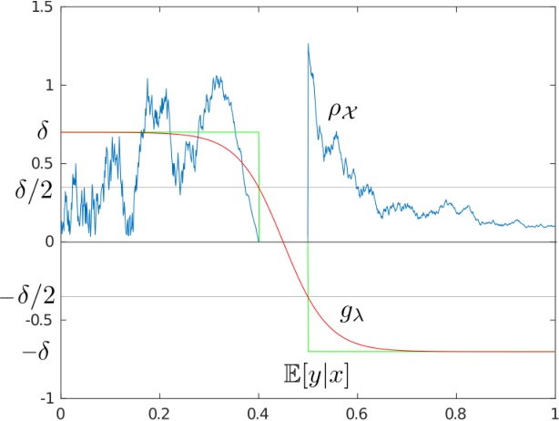
y_{i}=\begin{cases}\ \ \zeta_{i}&\textrm{if}~x_{i}\in S_{+}\\ -\zeta_{i}&\textrm{if}~x_{i}\in S_{-},\end{cases}

with $\zeta_{i}$ independently distributed as $\zeta_{i}=-1$ with probability $p\in[0,1/2)$ and $\zeta_{i}=1$ with probability $1-p$ . Then (A1) is satisfied with $\delta=1-2p$ and (A4) is satisfied as soon as (A2) and (A6) are, that is, the kernel is bounded and ${\mathcal{H}}$ is rich enough (see an example in Appendix E Figure 4).

Finally note that the results of this section can be easily generalized from ${\mathcal{X}}=\mathbb{R}^{d}$ to any Polish space, by using a separating kernel (De Vito et al., 2014; Rudi et al., 2014) instead of (A6).

4 Stochastic Gradient descent

We now consider the stochastic gradient algorithm to solve the ridge regression problem with a fixed strictly positive regularization parameter $\lambda$ . We consider solving the regularized problem with regularization $\|g-g_{0}\|_{{\mathcal{H}}}^{2}$ through stochastic approximation starting from a function $g_{0}\in{\mathcal{H}}$ (typically $0$ ).¹¹ 1 Note that $g_{0}$ is the initialization of the recursion, and is not the limit of $g_{\lambda}$ when $\lambda$ tends to zero (this limit being $\tilde{g}_{*}$ ). Denote by $F:\mathcal{H}\to\mathbb{R}$ , the functional

F(g)={\mathbb{E}}(Y-g(X))^{2}={\mathbb{E}}(Y-\langle K_{X},g\rangle)^{2},

where the last identity is due to the reproducing property of the RKHS $\mathcal{H}$ . Note that $F$ has the following gradient $\nabla F(g)=-2{\mathbb{E}}\left[(Y-\langle K_{X},g\rangle)K_{X}\right]$ . We consider also $F_{\lambda}=F+\lambda\|\cdot-g_{0}\|_{\mathcal{H}}^{2}$ , for which $\nabla F_{\lambda}(g)=\nabla F(g)+2\lambda(g-g_{0})$ , and we have for each pair of observation $(x_{n},y_{n})$ that $F_{\lambda}(g)={\mathbb{E}}\big[F_{n,\lambda}(g)\big]={\mathbb{E}}(\langle g,K_{x_{n}}\rangle-y_{n})^{2}+\lambda\|g-g_{0}\|_{\mathcal{H}}^{2}$ , with $F_{n,\lambda}(g)=(\langle g,K_{x_{n}}\rangle-y_{n})^{2}+\lambda\|g-g_{0}\|_{\mathcal{H}}^{2}$ .

Denoting $\Sigma={\mathbb{E}}\big[K_{x_{n}}\otimes K_{x_{n}}\big]$ the covariance operator defined as a linear operator from ${\mathcal{H}}$ to ${\mathcal{H}}$ (see Fukumizu et al., 2004, and references therein), we have the optimality conditions for $g_{\lambda}$ and $\tilde{g}_{*}$ :

\Sigma g_{\lambda}-{\mathbb{E}}\left(y_{n}K_{x_{n}}\right)+\lambda(g_{\lambda}-g_{0})=0,\qquad{\mathbb{E}}\left[\left(y_{n}-\tilde{g}_{*}(x_{n})\right)K_{x_{n}}\right]=0,

see Caponnetto and De Vito (2007) or Appendix F.1 for the proof of the last identity. Let $(\gamma_{n})_{n\geqslant 1}$ be a positive sequence; we consider the stochastic gradient recursion²² 2 The complexity of $n$ steps of the recursion is $O(n^{2})$ if using kernel functions or $O(\tau n)$ when using explicit feature representations, with $\tau$ the complexity of computing dot-products and adding feature vectors. in ${\mathcal{H}}$ started at $g_{0}$ :

\displaystyle{g}_{n}={g}_{n-1}-\frac{\gamma_{n}}{2}\nabla F_{n,\lambda}({g}_{n-1})={g}_{n-1}-\gamma_{n}\left[(\langle K_{x_{n}},{g}_{n-1}\rangle-y_{n})K_{x_{n}}+\lambda({g}_{n-1}-g_{0})\right].

(1)

We are going to consider Polyak-Ruppert averaging (Polyak and Juditsky, 1992), that is $\bar{g}_{n}=\frac{1}{n+1}\sum_{i=0}^{n}g_{i}$ , as well as the tail-averaging estimate $\bar{g}_{n}^{\textrm{tail}}=\frac{1}{\lfloor n/2\rfloor}\sum_{i=\lfloor n/2\rfloor}^{n}g_{i}$ , studied by Jain et al. (2016). For the sake of clarity, all the results in the main text are for the tail averaged estimate but note that all of them have been also proved for the full average in Appendix I.

As explained earlier (see Lemma 1), we need to show the convergence of ${g}_{n}$ to $g_{\lambda}$ in ${\mathcal{H}}$ -norm. We are going to consider two cases: (1) for the non-averaged recursion $(\gamma_{n})$ is a decreasing sequence, with the important particular case $\gamma_{n}=\gamma/n^{\alpha}$ , for $\alpha\in[0,1]$ ; (2) for the averaged or tail-averaged functions $(\gamma_{n})$ is a constant sequence equal to $\gamma$ . For all the proofs of this section see Appendix G. In the next subsection we reformulate the recursion in Eq. (1) as a least-squares recursion converging to $g_{\lambda}$ .

4.1 Reformulation as noisy recursion

We can first reformulate the SGD recursion equation in Eq. (1) as a regular least-squares SGD recursion with noise, with the notation $\xi_{n}=y_{n}-\tilde{g}_{*}(x_{n})$ , which satisfies ${\mathbb{E}}\big[\xi_{n}K_{x_{n}}\big]=0$ . This is the object of the following lemma (for the proof see Appendix F.2.):

Lemma 5.

The SGD recursion can be rewritten as follows:

\displaystyle{g}_{n}-g_{\lambda}=\big[I-\gamma_{n}(K_{x_{n}}\otimes K_{x_{n}}+\lambda I)\big]({g}_{n-1}-g_{\lambda})+\gamma_{n}\varepsilon_{n},

(2)

with the noise term $\varepsilon_{k}=\xi_{k}K_{x_{k}}+(\tilde{g}_{*}(x_{k})-g_{\lambda}(x_{k}))K_{x_{k}}-{\mathbb{E}}\left[(\tilde{g}_{*}(x_{k})-g_{\lambda}(x_{k}))K_{x_{k}}\right]\in{\mathcal{H}}.$

We are thus in presence of a least-squares problem in the Hilbert space ${\mathcal{H}}$ , to estimate a function $g_{\lambda}\in{\mathcal{H}}$ with a specific noise $\varepsilon_{n}$ in the gradient and feature vector $K_{x}$ . In the next section, we will consider the generic recursion above, which will require some bounds on the noise. In our setting, we have the following almost sure bounds and the noise (see Lemma 23 of Appendix G):

	$\displaystyle\\|\varepsilon_{n}\\|_{\mathcal{H}}$	$\displaystyle\leqslant R(1+2\\|\tilde{g}_{*}-g_{\lambda}\\|_{L_{\infty}})$
	$\displaystyle{\mathbb{E}}\big[\varepsilon_{n}\otimes\varepsilon_{n}\big]$	$\displaystyle\preccurlyeq 2\left(1+\\|\tilde{g}_{*}-g_{\lambda}\\|^{2}_{\infty}\right)\Sigma,$

where $\Sigma={\mathbb{E}}\big[K_{x_{n}}\otimes K_{x_{n}}\big]$ is the covariance operator.

4.2 SGD for general Least-Square problems

We now consider results on (averaged) SGD for least-squares that are interesting on their own. As said before, we show results in two different settings depending on the step-size sequence. First, we consider $(\gamma_{n})$ as a decreasing sequence, second we take $(\gamma_{n})$ constant but prove the convergence of the (tail-)averaged iterates.

Since the results we need could be of interest (even for finite-dimensional models), in this section, we study the following general recursion:

\displaystyle\eta_{n}=(I-\gamma H_{n})\eta_{n-1}+\gamma_{n}\varepsilon_{n},

(3)

We make the following assumptions:

(H ) 1.

We start at some $\eta_{0}\in{\mathcal{H}}$ .

(H ) 2.

$(H_{n},\varepsilon_{n})_{n\geqslant 1}$ are i.i.d. and $H_{n}$ is a positive self-adjoint operator so that almost surely $H_{n}\succcurlyeq\lambda I$ , and $H:={\mathbb{E}}H_{n}$ .

(H ) 3.

Noise: ${\mathbb{E}}\varepsilon_{n}=0$ , $\|\varepsilon_{n}\|_{\mathcal{H}}\leqslant c^{1/2}$ almost surely and ${\mathbb{E}}(\varepsilon_{n}\otimes\varepsilon_{n})\preccurlyeq C$ , with $C$ commuting with $H$ . Note that one consequence of this assumption is ${\mathbb{E}}\|\varepsilon_{n}\|_{\mathcal{H}}^{2}\leqslant\operatorname{Tr}C$ .

(H ) 4.

For all $n\geqslant 1$ , ${\mathbb{E}}\Big[H_{n}CH^{-1}H_{n}\Big]\preccurlyeq\gamma_{0}^{-1}C$ and $\gamma\leqslant\gamma_{0}$ .

(H ) 5.

$A$ is a positive self-adjoint operator which commutes with $H$ .

Note that we will later apply the results of this section to $H_{n}=K_{x_{n}}\otimes K_{x_{n}}+\lambda I$ , $H=\Sigma+\lambda I$ , $C=\Sigma$ and $A\in\{I,\Sigma\}$ . We first consider the non-averaged SGD recursion, then the (tail-)averaged recursion. The key difference with existing bounds is the need for precise probabilistic deviation results.

For least-squares, one can always separate the impact of the initial condition $\eta_{0}$ and of the noise terms $\varepsilon_{k}$ , namely $\eta_{n}=\eta_{n}^{\textrm{bias}}+\eta_{n}^{\textrm{variance}}$ , where $\eta_{n}^{\textrm{bias}}$ is the recursion with no noise ( $\varepsilon_{k}=0$ ), and $\eta_{n}^{\textrm{variance}}$ is the recursion started at $\eta_{0}=0$ . The final performance will be bounded by the sum of the two separate performances (Défossez and Bach, 2015, see, e.g.,). Hence all of our bounds will depend on these two. See more details in Appendix G.

4.3 Non-averaged SGD

In this section, we prove results for the recursion defined by Eq. (3) in the case where for $\alpha\in[0,1]$ , $\gamma_{n}=\gamma/n^{\alpha}$ . These results extend the ones of Bach and Moulines (2011) by providing deviation inequalities, but are limited to least-squares. For general loss functions and in the strongly-convex case, see also Kakade and Tewari (2009).

Theorem 6 (SGD, decreasing step size: $\gamma_{n}=\gamma/n^{\alpha}$ ).

Assume (H1), (H2), (H3), $\gamma_{n}=\gamma/n^{\alpha}$ , $\gamma\lambda<1$ and denote by $\eta_{n}\in{\mathcal{H}}$ the n-th iterate of the recursion in Eq. (3). We have for $t>0,n\geqslant 1$ and $\alpha\in(0,1)$ , $\|g_{n}-g_{\lambda}\|_{\mathcal{H}}\leqslant\exp\left(-\frac{\gamma\lambda}{1-\alpha}\left((n+1)^{1-\alpha}-1\right)\right)\|g_{0}-g_{\lambda}\|_{\mathcal{H}}+V_{n}$ , almost surely for $n$ large enough ³³ 3 See Appendix Section G Lemma 20 for more details., with $\displaystyle{\mathbb{P}}\left(V_{n}\geqslant t\right)\leqslant 2\exp\left(-\frac{t^{2}}{8\gamma\operatorname{Tr}C/\lambda+\gamma c^{1/2}t}\cdot n^{\alpha}\right).$

We can make the following observations:

•

The proof technique (see Appendix G.1 for the detailed proof) relies on the following scheme: we notice that $\eta_{n}$ can be decomposed in two terms, (a) the bias: obtained from a product of $n$ contractant operators, and (b) the variance: a sum of increments of a martingale. We treat separately the two terms. For the second one, we prove almost sure bounds on the increments and on the variance that lead to a Bernstein-type concentration result on the tail ${\mathbb{P}}(V_{n}\geqslant t)$ . Following this proof technique, the coefficient in the latter exponential is composed of the variance bound plus the almost sure bound of the increments of martingale times $t$ .
•

Note that we only presented in Theorem 6 the case where $\alpha\in(0,1)$ . Indeed, we only focused on the case where we had exponential convergence (see the whole result in the Appendix: Proposition 21). Actually, that there are three different regimes. For $\alpha=0$ (constant step-size), the algorithm is not converging, as the tail probability bound on ${\mathbb{P}}\left(V_{n}\geqslant t\right)$ is not dependent on $n$ . For $\alpha=1$ , confirming results from Bach and Moulines (2011), there is no exponential forgetting of initial conditions. And for $\alpha\in(0,1)$ , the forgetting of initial conditions and the tail probability are converging to zero exponentially fast, respectively, as $\exp(-Cn^{1-\alpha})$ and $\exp(-Cn^{\alpha})$ , for a constant $C$ , hence the natural choice of $\alpha=1/2$ in our experiments.

4.4 Averaged and Tail-averaged SGD with constant step-size

In the subsection, we take: $\forall n\geqslant 1,\ \gamma_{n}=\gamma$ . We first start with a result on the variance term, whose proof extends the work of Dieuleveut et al. (2017) to deviation inequalities which are sharper than the ones from Bach and Moulines (2013).

Theorem 7 (Convergence of the variance term in averaged SGD).

Assume (H1), (H2), (H3), (H4), (H5) and consider the average of the $n+1$ first iterates of the sequence defined in Eq. (3): $\bar{\eta}_{n}=\frac{1}{n+1}\sum_{i=0}^{n}\eta_{i}$ . Assume $\eta_{0}=0$ . We have for $t>0,n\geqslant 1$ :

\displaystyle{\mathbb{P}}\left(\left\|A^{1/2}\bar{\eta}_{n}\right\|_{\mathcal{H}}\geqslant t\right)\leqslant 2\exp\left[-\frac{(n+1)t^{2}}{E_{t}}\right],

(4)

where $E_{t}$ is defined with respect to the constants introduced in the assumptions:

E_{t}=4\operatorname{Tr}(AH^{-2}C)+\frac{2c^{1/2}\|A^{1/2}\|_{\textrm{op}}}{3\lambda}\cdot t.

(5)

The work that remains to be done is to bound the bias term of the recursion $\bar{\eta}_{n}^{\textrm{bias}}$ . We have done it for the full averaged sequence (see Appendix I.1 Theorem 25) but as it is quite technical and could lower a bit the clarity of the reasoning, we have decided to leave it in the Appendix. We present here another approach and consider the tail-averaged recursion, $\bar{\eta}_{n}^{\textrm{tail}}=\frac{1}{\lfloor n/2\rfloor}\sum_{i=\lfloor n/2\rfloor}^{n}\eta_{i}$ (Jain et al., 2016; Shamir, 2011, as proposed by). For this, we use the simple almost sure bound $\|\eta_{i}^{\textrm{bias}}\|_{\mathcal{H}}\leqslant(1-\lambda\gamma)^{i}\|\eta_{0}\|_{\mathcal{H}}$ , such that $\|\bar{\eta}_{n}^{\textrm{tail, bias}}\|_{\mathcal{H}}\leqslant(1-\lambda\gamma)^{n/2}\|\eta_{0}\|_{\mathcal{H}}$ . For the variance term, we can simply use the result above for $n$ and $n/2$ , as $\bar{\eta}_{n}^{\textrm{tail}}=2\bar{\eta}_{n}-\bar{\eta}_{n/2}$ . This leads to:

Corollary 8 (Convergence of tail-averaged SGD).

Assume (H1), (H2), (H3), (H4), (H5) and consider the tail-average of the sequence defined in Eq. (3): $\bar{\eta}_{n}^{\textrm{tail}}=\frac{1}{\lfloor n/2\rfloor}\sum_{i=\lfloor n/2\rfloor}^{n}\eta_{i}$ . We have for $t>0,n\geqslant 1$ :

	$\displaystyle\left\\|A^{1/2}\bar{\eta}_{n}^{\textrm{tail}}\right\\|_{\mathcal{H}}$	$\displaystyle\leqslant$	$\displaystyle(1-\gamma\lambda)^{n/2}\\|A^{1/2}\\|_{op}\\|\eta_{0}\\|_{\mathcal{H}}+L_{n}\quad,\ \text{with}$		(6)
	$\displaystyle{\mathbb{P}}(L_{n}\geqslant t)$	$\displaystyle\leqslant$	$\displaystyle 4\exp\left(-(n+1)t^{2}/(4E_{t})\right),$		(7)

where $L_{n}$ is defined in the proof (see Appendix G.3) and is the variance term of the tail-averaged recursion.

We can make the following observations on the two previous results:

•

The proof technique (see Appendix G.2 and G.3 for the detailed proofs) relies on concentration inequality of Bernstein type. Indeed, we notice that (in the setting of Theorem 7) $\bar{\eta}_{n}$ is a sum of increments of a martingale. We prove almost sure bounds on the increments and on the variance (Dieuleveut et al., 2017, following the proof technique of) that lead to a Bernstein type concentration result on the tail ${\mathbb{P}}(V_{n}\geqslant t)$ . Following the proof technique summed-up before, we see that $E_{t}$ is composed of the variance bound plus the almost sure bound times $t$ .
•

Remark that classically, $A$ and $C$ are proportional to $H$ for excess risk predictions. In the finite $d$ -dimensional setting this leads us to the usual variance bound proportional to the dimension $d$ : $\operatorname{Tr}(AH^{-2}C)\cong\operatorname{Tr}I=d$ . The result is general in the sense that we can apply it for all matrices $A$ commuting with $H$ (this can be used to prove results in $L_{2}$ or in ${\mathcal{H}}$ ).
•

Finally, note that we improved the variance bound with respect to the strong convexity parameter $\lambda$ which is usually of the order $1/\lambda^{2}$ (Shamir, 2011, see), and is here $\operatorname{Tr}(AH^{-2}C)$ . Indeed, in our setting, we will apply it for $A=C=\Sigma$ and $H=\Sigma+\lambda I$ , so that $\operatorname{Tr}(AH^{-2}C)$ is upper bounded by the effective dimension $\operatorname{Tr}(\Sigma(\Sigma+\lambda I)^{-1})$ which can be way smaller than $1/\lambda^{2}$ (Caponnetto and De Vito, 2007; Dieuleveut and Bach, 2016, see).
•

The complete proof for the full average is written in Appendix I.1 and more precisely in Theorem 25. In this case the initial conditions are not forgotten exponentially fast though.

5 Exponentially Convergent SGD for Classification error

In this section we want to show our main results, on the error made (on unseen data) by the $n$ -th iterate of the regularized SGD algorithm. Hence, we go back to the original SGD recursion defined in Eq. (2). Let us recall it:

{g}_{n}-g_{\lambda}=\big[I-\gamma_{n}(K_{x_{n}}\otimes K_{x_{n}}+\lambda I)\big]({g}_{n-1}-g_{\lambda})+\gamma_{n}\varepsilon_{n},

with the noise term $\varepsilon_{k}=\xi_{k}K_{x_{k}}+(\tilde{g}_{*}(x_{k})-g_{\lambda}(x_{k}))K_{x_{k}}-{\mathbb{E}}\left[(\tilde{g}_{*}(x_{k})-g_{\lambda}(x_{k}))K_{x_{k}}\right]\in{\mathcal{H}}.$ Like in the previous section we are going to state two results in two different settings, the first one for SGD with decreasing step-size ( $\gamma_{n}=\gamma/n^{\alpha}$ ) and the second one for tail averaged SGD with constant step-size. For all the proofs of this section see the Appendix (section H).

5.1 SGD with decreasing step-size

In this section, we focus on decreasing step-sizes $\gamma_{n}=\gamma/n^{\alpha}$ for $\alpha\in(0,1)$ , which lead to exponential convergence rates. Results for $\alpha=1$ and $\alpha=0$ can be derived in a similar way (but do not lead to exponential rates).

Theorem 9.

Assume (A1), (A2), (A3), (A4) and $\gamma_{n}=\gamma/n^{\alpha}$ , $\alpha\in(0,1)$ for any $n$ and $\gamma\lambda<1$ . Let $g_{n}$ be the n-th iterate of the recursion defined in Eq. (2), as soon as $n$ satisfies the inequality $\exp\left(-\frac{\gamma\lambda}{1-\alpha}\left((n+1)^{1-\alpha}-1\right)\right)\leqslant\delta/(5R\|g_{0}-g_{\lambda}\|_{\mathcal{H}})$ , then

\displaystyle{\cal R}(g_{n})={\cal R}^{*},\mbox{ with probability at least }1-2\exp\left(-\frac{\delta^{2}}{C_{R}}\cdot n^{\alpha}\right),

with $C_{R}=2^{\alpha+7}\gamma R^{2}\operatorname{Tr}\Sigma\left(1+\|\tilde{g}_{*}-g_{\lambda}\|^{2}_{\infty}\right)/\lambda+8\gamma R^{2}\delta(1+2\|\tilde{g}_{*}-g_{\lambda}\|_{\infty})/3$ , and in particular

\mathbb{E}\left[{{\cal R}(g_{n})-{\cal R}^{*}}\right]\leqslant 2\exp\left(-\frac{\delta^{2}}{C_{R}}\cdot n^{\alpha}\right).

Note that Theorem 9 shows that with probability at least $1-2\exp\left(-\frac{\delta^{2}}{C_{R}}\cdot n^{\alpha}\right)$ , the predictions of $g_{n}$ are perfect. We can also make the following observations:

•

The idea of the proof (see Appendix H.1 for the detailed proof) is the following: we know that as soon as $\|g_{n}-g_{\lambda}\|_{\mathcal{H}}\leqslant\delta/(2R)$ , the predictions of $g_{n}$ are perfect (Lemma 1). We just have to apply Theorem 6 for to the original SGD recursion and make sure to bound each term by $\delta/(4R)$ . Similar results for non-averaged SGD could be derived beyond least-squares (e.g., hinge or logistic loss) using results from Kakade and Tewari (2009).
•

Also note that the larger the $\alpha$ , the smaller the bound. However, it is only valid for $n$ larger that a certain quantity depending of $\lambda\gamma$ . A good trade-off is $\alpha=1/2$ , for which we get an excess error of $2\exp\left(-\frac{\delta^{2}}{C_{R}}n^{1/2}\right)$ , which is valid as soon as $n\geqslant\log(10R\|g_{0}-g_{\lambda}\|_{\mathcal{H}}/\delta)/(4\lambda^{2}\gamma^{2})$ . Notice also that we should go for large $\gamma\lambda$ to increase the factor in the exponential and make the condition happen as soon as possible.
•

If we want to emphasize the dependence of the bound on the important parameters, we can write that: $\mathbb{E}\left[{{\cal R}(g_{n})-{\cal R}^{*}}\right]\lesssim 2\exp\left(-\lambda\delta^{2}n^{\alpha}/R^{2}\right).$
•

When the condition on $n$ is not met, then we still have the usual bound obtained by taking directly the excess loss (Bartlett et al., 2006) but we lose exponential convergence.

5.2 Tail averaged SGD with constant step-size

We now consider the tail-averaged recursion⁴⁴ 4 The full averaging result corresponding to Theorem 10 is proved in Appendix I.2, Theorem 26., with the following result:

Theorem 10.

Assume (A1), (A2), (A3), (A4) and $\gamma_{n}=\gamma$ for any n, $\gamma\lambda<1$ and $\gamma\leqslant\gamma_{0}=(R^{2}+2\lambda)^{-1}$ . Let $g_{n}$ be the n-th iterate of the recursion defined in Eq. (2), and $\bar{g}_{n}^{\textrm{tail}}=\frac{1}{\lfloor n/2\rfloor}\sum_{i=\lfloor n/2\rfloor}^{n}g_{i}$ , as soon as $n\geqslant 2/(\gamma\lambda)\ln(5R\|g_{0}-g_{\lambda}\|_{\mathcal{H}}/\delta)$ , then

{\cal R}(\bar{g}_{n}^{\textrm{tail}})={\cal R}^{*},\mbox{ with probability at least }1-4\exp\left(-\delta^{2}K_{R}(n+1)\right),

with $K_{R}^{-1}=2^{9}R^{2}\left(1+\|\tilde{g}_{*}-g_{\lambda}\|^{2}_{\infty}\right)\operatorname{Tr}(\Sigma(\Sigma+\lambda I)^{-2})+32\delta R^{2}(1+2\|\tilde{g}_{*}-g_{\lambda}\|_{\infty})/(3\lambda),$ and in particular

\mathbb{E}\left[{{\cal R}(\bar{g}_{n}^{\textrm{tail}})-{\cal R}^{*}}\right]\leqslant 4\exp\left(-\delta^{2}K_{R}(n+1)\right).

Theorem 10 shows that with probability at least $1-4\exp\left(-\delta^{2}K_{R}(n+1)\right)$ , the predictions of $\bar{g}_{n}^{\textrm{tail}}$ are perfect. We can also make the following observations:

•

The idea of the proof (see Appendix H.2 for the detailed proof) is the following: we know that as soon as $\|\bar{g}_{n}^{\textrm{tail}}-g_{\lambda}\|_{\mathcal{H}}\leqslant\delta/(2R)$ , the predictions of $\bar{g}_{n}^{\textrm{tail}}$ are perfect (Lemma 1). We just have to apply Corollary 8 to the original SGD recursion, and make sure to bound each term by $\delta/(4R)$ .
•

If we want to emphasize the dependence of the bound on the important parameters, we can write that: $\mathbb{E}\left[{{\cal R}(g_{n})-{\cal R}^{*}}\right]\lesssim 2\exp\left(-\lambda^{2}\delta^{2}n/R^{4}\right).$ Note that the $\lambda^{2}$ could be made much smaller with assumptions on the decrease of eigenvalues of $\Sigma$ (it has been shown Caponnetto and De Vito, 2007, that if the decay happens at speed $1/n^{\beta}$ : $\operatorname{Tr}\Sigma(\Sigma+\lambda I)^{-2}\leqslant\lambda^{-1}\operatorname{Tr}\Sigma(\Sigma+\lambda I)^{-1}\leqslant R^{2}/\lambda^{1+1/\beta}$ ).
•

We want to take $\gamma\lambda$ as big as possible to satisfy quickly the condition. In comparison to the convergence rate in the case of decreasing step-sizes, the dependence on $n$ is improved as the convergence is really an exponential of $n$ (and not of some power of $n$ as in the previous result).
•

Finally, the complete proof for the full average is contained in Appendix I.2 and more precisely in Theorem 26.

6 Conclusion

In this paper, we have shown that stochastic gradient could be exponentially convergent, once some margin conditions are assumed; and even if a weaker margin condition is assumed, fast rates can be achieved (see Appendix J). This is obtained by running averaged stochastic gradient on a least-squares problem, and proving new deviation inequalities.

Our work could be extended in several natural ways: (a) our work relies on new concentration results for the least-mean-squares algorithm (i.e., SGD for square loss), it is natural to extend it to other losses, such as the logistic or hinge loss; (b) going beyond binary classification is also natural with the square loss (Ciliberto et al., 2016; Osokin et al., 2017) or without (Taskar et al., 2005); (c) in our experiments, we use regularization, but we have experimented with unregularized recursions, which do exhibit fast convergence, but for which proofs are usually harder (Dieuleveut and Bach, 2016); finally, (d) in order to avoid the $O(n^{2})$ complexity, extending the results of Rudi et al. (2017); Rudi and Rosasco (2017) would lead to a subquadratic complexity.

acknowledgments-disclosure-of-funding.

We acknowledge support from the European Research Council (grant SEQUOIA 724063). We would like to thank Raphaël Berthier for useful discussions.

References

Adams and Fournier (2003) Robert A. Adams and John J.F. Fournier. Sobolev spaces, volume 140. Academic Press, 2003.
Audibert and Tsybakov (2007) Jean-Yves Audibert and Alexandre B. Tsybakov. Fast learning rates for plug-in classifiers. The Annals of statistics, 35(2):608–633, 2007.
Bach and Moulines (2011) F. Bach and E. Moulines. Non-asymptotic analysis of stochastic approximation algorithms for machine learning. In Advances in Neural Information Processing Systems (NIPS), 2011.
Bach and Moulines (2013) F. Bach and E. Moulines. Non-strongly-convex smooth stochastic approximation with convergence rate ${O}(1/n)$ . In Advances in Neural Information Processing Systems (NIPS), 2013.
Bartlett et al. (2006) Peter L. Bartlett, Michael I. Jordan, and Jon D. McAuliffe. Convexity, classification, and risk bounds. Journal of the American Statistical Association, 101(473):138–156, 2006.
Bottou and Le Cun (2005) L. Bottou and Y. Le Cun. On-line learning for very large data sets. Applied Stochastic Models in Business and Industry, 21(2):137–151, 2005.
Caponnetto and De Vito (2007) Andrea Caponnetto and Ernesto De Vito. Optimal rates for the regularized least-squares algorithm. Foundations of Computational Mathematics, 7(3):331–368, 2007.
Ciliberto et al. (2016) Carlo Ciliberto, Lorenzo Rosasco, and Alessandro Rudi. A consistent regularization approach for structured prediction. In Advances in Neural Information Processing Systems, 2016.
De Vito et al. (2014) Ernesto De Vito, Lorenzo Rosasco, and Alessandro Toigo. Learning sets with separating kernels. Applied and Computational Harmonic Analysis, 37(2):185–217, 2014.
Defazio et al. (2014) Aaron Defazio, Francis Bach, and Simon Lacoste-Julien. SAGA: A fast incremental gradient method with support for non-strongly convex composite objectives. In Advances in Neural Information Processing Systems, 2014.
Défossez and Bach (2015) A. Défossez and F. Bach. Constant step size least-mean-square: Bias-variance trade-offs and optimal sampling distributions. In Proc. AISTATS, 2015.
Devroye et al. (2013) Luc Devroye, László Györfi, and Gábor Lugosi. A Probabilistic Theory of Pattern Recognition, volume 31. Springer Science & Business Media, 2013.
Dieuleveut and Bach (2016) Aymeric Dieuleveut and Francis Bach. Nonparametric stochastic approximation with large step-sizes. The Annals of Statistics, 44(4):1363–1399, 2016.
Dieuleveut et al. (2017) Aymeric Dieuleveut, Nicolas Flammarion, and Francis Bach. Harder, better, faster, stronger convergence rates for least-squares regression. Journal of Machine Learning Research, pages 1–51, 2017.
Fukumizu et al. (2004) Kenji Fukumizu, Francis Bach, and Michael I. Jordan. Dimensionality reduction for supervised learning with reproducing kernel Hilbert spaces. Journal of Machine Learning Research, 5(Jan):73–99, 2004.
Jain et al. (2016) Prateek Jain, Sham M. Kakade, Rahul Kidambi, Praneeth Netrapalli, and Aaron Sidford. Parallelizing stochastic approximation through mini-batching and tail-averaging. Technical Report 1610.03774, arXiv, 2016.
Johnson and Zhang (2013) R. Johnson and T. Zhang. Accelerating stochastic gradient descent using predictive variance reduction. In Advances in Neural Information Processing Systems, 2013.
Kakade and Tewari (2009) Sham M. Kakade and Ambuj Tewari. On the generalization ability of online strongly convex programming algorithms. In Advances in Neural Information Processing Systems, 2009.
Koltchinskii and Beznosova (2005) Vladimir Koltchinskii and Olexandra Beznosova. Exponential convergence rates in classification. In International Conference on Computational Learning Theory. Springer, 2005.
Le Roux et al. (2012) Nicolas Le Roux, Mark Schmidt, and Francis Bach. A stochastic gradient method with an exponential convergence rate for finite training sets. In Advances in Neural Information Processing Systems, 2012.
Mammen and Tsybakov (1999) Enno Mammen and Alexandre Tsybakov. Smooth discrimination analysis. The Annals of Statistics, 27(6):1808–1829, 1999.
Nemirovski et al. (2009) A. Nemirovski, A. Juditsky, G. Lan, and A. Shapiro. Robust stochastic approximation approach to stochastic programming. SIAM Journal on Optimization, 19(4):1574–1609, 2009.
Nemirovski and Yudin (1983) A. S. Nemirovski and D. B. Yudin. Problem complexity and method efficiency in optimization. John Wiley, 1983.
Nesterov and Vial (2008) Y. Nesterov and J. P. Vial. Confidence level solutions for stochastic programming. Automatica, 44(6):1559–1568, 2008.
Osokin et al. (2017) Anton Osokin, Francis Bach, and Simon Lacoste-Julien. On structured prediction theory with calibrated convex surrogate losses. In Advances in Neural Information Processing Systems, 2017.
Pinelis (1994) Iosif Pinelis. Optimum bounds for the distributions of martingales in banach spaces. The Annals of Probability, pages 1679–1706, 1994.
Polyak and Juditsky (1992) B. T. Polyak and A. B. Juditsky. Acceleration of stochastic approximation by averaging. SIAM Journal on Control and Optimization, 30(4):838–855, 1992.
Robbins and Monro (1951) H. Robbins and S. Monro. A stochastic approximation method. Ann. Math. Statistics, 22:400–407, 1951.
Rosasco et al. (2010) Lorenzo Rosasco, Mikhail Belkin, and Ernesto De Vito. On learning with integral operators. Journal of Machine Learning Research, 11(Feb):905–934, 2010.
Rudi and Rosasco (2017) Alessandro Rudi and Lorenzo Rosasco. Generalization properties of learning with random features. In Advances in Neural Information Processing Systems, 2017.
Rudi et al. (2014) Alessandro Rudi, Guillermo D Canas, Ernesto De Vito, and Lorenzo Rosasco. Learning sets and subspaces. Regularization, Optimization, Kernels, and Support Vector Machines, pages 337–357, 2014.
Rudi et al. (2017) Alessandro Rudi, Luigi Carratino, and Lorenzo Rosasco. FALKON: An optimal large scale kernel method. In Advances in Neural Information Processing Systems 30. 2017.
Schmidt and Le Roux (2013) Mark Schmidt and Nicolas Le Roux. Fast convergence of stochastic gradient descent under a strong growth condition. Technical Report 1308.6370, arXiv, 2013.
Schölkopf and Smola (2002) B. Schölkopf and A. J. Smola. Learning with Kernels. MIT Press, 2002.
Shalev-Shwartz et al. (2007) S. Shalev-Shwartz, Y. Singer, and N. Srebro. Pegasos: Primal estimated sub-gradient solver for svm. In Proceedings of the International Conference on Machine Learning (ICML), 2007.
Shamir (2011) Ohad Shamir. Making gradient descent optimal for strongly convex stochastic optimization. CoRR, abs/1109.5647, 2011.
Shawe-Taylor and Cristianini (2004) J. Shawe-Taylor and N. Cristianini. Kernel Methods for Pattern Analysis. Cambridge University Press, 2004.
Solodov (1998) Mikhail V Solodov. Incremental gradient algorithms with stepsizes bounded away from zero. Computational Optimization and Applications, 11(1):23–35, 1998.
Taskar et al. (2005) B. Taskar, V. Chatalbashev, D. Koller, and C. Guestrin. Learning structured prediction models: A large margin approach. In Proceedings of the International Conference on Machine Learning (ICML), 2005.
Xiao (2010) L. Xiao. Dual averaging methods for regularized stochastic learning and online optimization. Journal of Machine Learning Research, 9:2543–2596, 2010.
Yao et al. (2007) Yuan Yao, Lorenzo Rosasco, and Andrea Caponnetto. On early stopping in gradient descent learning. Constructive Approximation, 26(2):289–315, 2007.
Zhang (2004) Tong Zhang. Statistical behavior and consistency of classification methods based on convex risk minimization. Annals of Statistics, pages 56–85, 2004.

Organization of the Appendix

A.

Experiments
where the experiments and their settings are explained.
B.

Probabilistic lemmas
where concentration inequalities in Hilbert spaces used in section G are recalled.
C.

From ${\mathcal{H}}$ to 0-1 loss
where, from high probability bound for $\|\cdot\|_{\mathcal{H}}$ , we derived bound for the 0-1 error.
D.

Proofs of Exponential rates for Kernel Ridge Regression
where exponential rates for Kernel Ridge Regression are proven (Theorem 14).
E.

Proofs and additional results about concrete examples
where additional results and croncrete examples to satisfy (A4) are given.
F.

Preliminaries for Stochastic Gradient Descent
where the SGD recursion is derived.
G.

Proof of stochastic gradient descent results
where high probability bounds for the general SGD recursion are shown (Theorems 6 and 7).
H.

Exponentially convergent SGD for classification error
where exponential convergence of test error are shown (Theorems 9 and 10).
I.

Extension for the full averaged case
where previous results are extended for full averaged SGD (instead of tail-averaged).
J.

Convergence under weaker margin assumption
where previous results are extended in the case of a weaker margin assumption.

Appendix A Experiments

To illustrate our results, we consider one-dimensional synthetic examples ( ${\mathcal{X}}=[0,1]$ ) for which our assumptions are easily satisfied. Indeed, we consider the following set-up that fulfils our assumptions:

•

(A1), (A3) We consider here $X\sim U\left([0,(1-\varepsilon)/2]\cup[(1+\varepsilon)/2,1]\right)$ and with the notations of Example 4, we take $\mathcal{S}_{+}=[0,(1-\varepsilon)/2]$ and $\mathcal{S}_{-}=[(1+\varepsilon)/2,1]$ . For $1\leq i\leq n$ , $x_{i}$ independently sampled from ${\rho_{{\mathcal{X}}}}$ we define $y_{i}=1$ if $x_{i}\in\mathcal{S}_{+}$ and $y_{i}=-1$ if $x_{i}\in\mathcal{S}_{-}$ .
•

(A2) We take the kernel to be the exponential kernel $K(x,x^{\prime})=\exp(-|x-x^{\prime}|)$ for which the RKHS is a Sobolev space ${\mathcal{H}}=W^{s,2}$ , with $s>d/2$ , which is dense in $L_{2}$ (Adams and Fournier, 2003).

•

(A4) With this setting we could find a closed form for $g_{\lambda}$ and checked that it verified (A4). Indeed we could solve the optimality equation satisfied by $g_{\lambda}$ :

\forall z\in[0,1],\ \int_{0}^{1}K(x,z)g_{\lambda}(x)d\rho_{X}(x)+\lambda g_{\lambda}(z)=\int_{0}^{1}K(x,z)g_{\rho}(x)d\rho_{X}(x),

the solution being a linear combination of exponentials in each set : $[0,(1-\varepsilon)/2]$ , $[(1-\varepsilon)/2,(1+\varepsilon)/2]$ and $[(1+\varepsilon)/2,1]$ .

Figure 1: Representing the

\rho_{\mathcal{X}}

density (uniform with

\varepsilon

-margin), the best estimator, i.e.,

{\mathbb{E}}(x|y)

and

g_{\lambda}

used for the simulations (

\lambda=0.01

In the case of SGD with decreasing step size, we computed only the test error $\mathbb{E}({\cal R}(g_{n})-{\cal R}^{*}))$ . For tail averaged SGD with constant step size, we computed the test error as well as the training error, the test loss (which corresponds to the $L_{2}$ loss : $\int_{0}^{1}(g_{n}(x)-g_{\lambda}(x))^{2}d\rho(x)$ ) and the training loss. In all cases we computed the errors of the $n$ -th iterate with respect to the calculated $g_{\lambda}$ , taking $g_{0}=0$ . For any $n\geqslant 1$ ,

g_{n}={g}_{n-1}-\gamma_{n}\big[({g}_{n-1}(x_{n})-y_{n})K_{x_{n}}+\lambda{g}_{n-1}\big].

We can use representants to find the recursion on the coefficients. Indeed, if $g_{n}=\sum_{i=1}^{n}a^{n}_{i}K_{x_{i}},$ then the following recursion for the $(a_{i}^{n})$ reads :

	$\displaystyle\text{for }i\leqslant n-1,\ a_{i}^{n}$	$\displaystyle=$	$\displaystyle(1-\gamma_{n}\lambda)a_{i}^{n-1}$
	$\displaystyle a_{n}^{n}$	$\displaystyle=$	$\displaystyle-\gamma_{n}(\sum_{i=1}^{n-1}a_{i}^{n-1}K(x_{n},x_{i})-y_{n}).$

From $(a_{i}^{n})$ , we can also compute the coefficients of $\bar{g}_{n}$ and $\bar{g}_{n}^{\textrm{tail}}$ that we note $\bar{a}^{n}_{i}$ and $\bar{a}^{n,\textrm{tail}}_{i}$ respectively: $\bar{a}^{n}_{i}=\sum_{k=i}^{n}\frac{a_{i}^{k}}{n+1}$ and $\bar{a}^{n,\textrm{tail}}_{i}=\frac{1}{\lfloor n/2\rfloor}\sum_{k=\lfloor n/2\rfloor}^{n}a_{i}^{k}.$ To show our theoretical results we have decided to present the following figures:

•

For the exponential convergence of the averaged and tail averaged cases, we plotted the error $\log_{10}\mathbb{E}({\cal R}(g_{n})-{\cal R}^{*}))$ as a function of $n$ . With this scale and following our results it goes as a line after a certain $n$ (Figures 2 and 3 right).
•

We recover the results of Dieuleveut et al. (2017) that show convergence at speed $1/n$ for the loss (Figure 2 left). We adapted the scale to compare with the error plot.
•

For Figure 3 left, we plotted $-\log(-\log(\mathbb{E}({\cal R}(g_{n})-{\cal R}^{*})))$ of the excess error with respect to the $\log$ of $n$ to show a line of slope $-1/2$ . It meets our theoretical bound of the form $\exp(-K\sqrt{n})$ ,

Note that for the plots where we plotted the expected excess errors, i.e., $\mathbb{E}({\cal R}(g_{n})-{\cal R}^{*})$ , we plotted the mean of the errors over 1000 replications until $n=200$ , whereas for the plots where we plotted the losses, i.e., a function of $\|g_{n}-g_{*}\|_{2}$ , we plotted the mean of the loss over 100 replications until $n=2000$ .

Figure 2: Showing linear convergence for the

L^{01}

errors in the case of margin of width

\varepsilon

. Left figure corresponds to the test and training loss in the averaged case whereas the right one corresponds to the error in the same setting. Note that the y-axis is the same while the x-axis is different of a factor 10. The fact that the error plot is a line after a certain

n

matches our theoretical results. We took the following parameters :

\varepsilon=0.05

\gamma=0.25

\lambda=0.01

We can make the following observations:

First remark that between plots of losses and errors (Figure 2 left and right resp.), there is a factor 10 between the numbers of samples (200 for errors and 2000 for losses) and another factor 10 between errors and losses ( $10^{-4}$ for errors and $10^{-3}$ for losses). That underlines well our theoretical result which is the difference between exponential rates of convergence of the excess error and $1/n$ rate of convergence of the loss.

Figure 3: Left plot shows the error in the non-averaged case for

\gamma_{n}=\gamma/\sqrt{n}

and right compares the test error between averaged and tail averaged case. We took the following parameters :

\varepsilon=0.05

\gamma=0.25

\lambda=0.01

Moreover, we see that even if the excess error with tail averaging seems a bit faster, we have linear rates too for the convergence of the excess error in the averaged case. Finally, we remark that the error on the train set is always below the one for a unknown test set (of what seems to be close to a factor 2).

Appendix B Probabilistic lemmas

In this section we recall two fundamental results for concentration inequalities in Hilbert spaces shown in Pinelis (1994).

Proposition 11.

Let $(X_{k})_{k\in\mathbb{N}}$ be a sequence of vectors of $\mathcal{H}$ adapted to a non decreasing sequence of $\sigma$ -fields $(\mathcal{F}_{k})$ such that ${\mathbb{E}}\left[X_{k}|\mathcal{F}_{k-1}\right]=0$ , $\sup_{k\leqslant n}\|X_{k}\|\leqslant a_{n}$ and $\sum_{k=1}^{n}{\mathbb{E}}\left[\|X_{k}\|^{2}|\mathcal{F}_{k-1}\right]\leqslant b_{n}^{2}$ for some sequences $(a_{n}),(b_{n})\in\left(\mathbb{R}_{+}^{*}\right)^{\mathbb{N}}$ . Then, for all $t\geqslant 0$ , $n\geqslant 1$ ,

\displaystyle{\mathbb{P}}\left(\left\|\sum_{k=1}^{n}X_{k}\right\|\geqslant t\right)\leqslant 2\exp\left(\frac{t}{a_{n}}-\left(\frac{t}{a_{n}}+\frac{b_{n}^{2}}{a_{n}^{2}}\right)\ln\left(1+\frac{ta_{n}}{b_{n}}\right)\right).

(8)

Proof.

As ${\mathbb{E}}\left[X_{k}|\mathcal{F}_{k-1}\right]=0$ , the $\mathcal{F}_{j}$ -adapted sequence $(f_{j})$ defined by $f_{j}=\sum_{k=1}^{j}X_{k}$ is a martingale and so is the stopped-martingale $(f_{j\wedge n})$ . By applying Theorem 3.4 of Pinelis (1994) to the martingale $(f_{j\wedge n})$ , we have the result. ∎

Corollary 12.

\displaystyle{\mathbb{P}}\left(\left\|\sum_{k=1}^{n}X_{k}\right\|\geqslant t\right)\leqslant 2\exp\left(-\frac{t^{2}}{2\left(b_{n}^{2}+a_{n}t/3\right)}\right).

(9)

Proof.

We apply 11 and simply notice that

	$\displaystyle\frac{t}{a_{n}}-\left(\frac{t}{a_{n}}+\frac{b_{n}^{2}}{a_{n}^{2}}\right)\ln\left(1+\frac{ta_{n}}{b_{n}}\right)$	$\displaystyle=$	$\displaystyle-\frac{b_{n}^{2}}{a_{n}^{2}}\left(\left(1+\frac{a_{n}t}{b_{n}^{2}}\right)\ln\left(1+\frac{a_{n}t}{b_{n}^{2}}\right)-\frac{a_{n}t}{b_{n}^{2}}\right)$
		$\displaystyle=$	$\displaystyle-\frac{b_{n}^{2}}{a_{n}^{2}}\phi\left(\frac{a_{n}t}{b_{n}^{2}}\right),$

where $\phi(u)=(1+u)\ln(1+u)-u$ for $u>0$ . Moreover $\phi(u)\geqslant\displaystyle\frac{u^{2}}{2\left(1+u/3\right)}$ , so that:

\displaystyle\frac{t}{a_{n}}-\left(\frac{t}{a_{n}}+\frac{b_{n}^{2}}{a_{n}^{2}}\right)\ln\left(1+\frac{ta_{n}}{b_{n}}\right)\leqslant-\frac{b_{n}^{2}}{a_{n}^{2}}\frac{(a_{n}t/b_{n}^{2})^{2}}{2\left(1+a_{n}t/3b_{n}^{2}\right)}=-\frac{t^{2}}{2\left(b_{n}^{2}+a_{n}t/3\right)}.

∎

Appendix C From ${\mathcal{H}}$ to 0-1 loss

In this section we prove Lemma 1. Note that (A4) requires the existence of $g_{\lambda}$ having the same sign of $g_{\ast}$ almost everywhere on the support of ${\rho_{{\mathcal{X}}}}$ and with absolute value uniformly bounded from below. In Lemma 1 we prove that we can bound the 0-1 error with respect to the distance in $\mathcal{H}$ of the estimator $\widehat{g}$ form $g_{\lambda}$ .

Proof.

of Lemma 1 Denote by $W$ the event such that $\bigl\|{\widehat{g}-g_{\lambda}}\bigr\|_{\mathcal{H}}<\delta/(2R)$ . Note that for any $f\in\mathcal{H}$ ,

f(x)=\left\langle{f},{K_{x}}\right\rangle_{\mathcal{H}}\leq\bigl\|{K_{x}}\bigr\|_{\mathcal{H}}\bigl\|{f}\bigr\|_{\mathcal{H}}\leq R\bigl\|{f}\bigr\|_{\mathcal{H}},

for any $x\in{\mathcal{X}}$ . So for $\widehat{g}\in W$ , we have

|\widehat{g}(x)-g_{\lambda}(x)|\leq R\bigl\|{\widehat{g}-g_{\lambda}}\bigr\|_{\mathcal{H}}<\delta/2\quad\forall x\in{\mathcal{X}}.

Let $x$ be in the support of ${\rho_{{\mathcal{X}}}}$ . By (A4) $|g_{\lambda}(x)|\geq\delta/2$ a.e.. Let $\widehat{g}\in W$ and $x\in{\mathcal{X}}$ such that $g_{\lambda}(x)>0$ , we have

\widehat{g}(x)=g_{\lambda}(x)-(g_{\lambda}(x)-\widehat{g}(x))\geq g_{\lambda}(x)-|g_{\lambda}(x)-\widehat{g}(x)|>0,

so $\mathop{\mathrm{sign}}(\widehat{g}(x))=\mathop{\mathrm{sign}}(g_{\lambda}(x))=+1$ . Similarly let $\widehat{g}\in W$ and $x\in{\mathcal{X}}$ such that $g_{\lambda}(x)<0$ , we have

\widehat{g}(x)=g_{\lambda}(x)+(\widehat{g}(x)-g_{\lambda}(x))\leq g_{\lambda}(x)+|g_{\lambda}(x)-\widehat{g}(x)|<0,

so $\mathop{\mathrm{sign}}(\widehat{g}(x))=\mathop{\mathrm{sign}}(g_{\lambda}(x))=-1$ . Finally note that for any $\widehat{g}\in\mathcal{H}$ , by (A4), either $g_{\lambda}(x)>0$ or $g_{\lambda}(x)<0$ a.e., so $\mathop{\mathrm{sign}}(\widehat{g}(x))=\mathop{\mathrm{sign}}(g_{\lambda}(x))$ a.e.

Now note that by (A1), (A4) we have that $\mathop{\mathrm{sign}}(g_{\ast}(x))=\mathop{\mathrm{sign}}(g_{\lambda}(x))$ a.e., where $g_{\ast}(x):=\mathbb{E}\left({y}\middle|{x}\right)$ . So when $\widehat{g}\in W$ , we have that $\mathop{\mathrm{sign}}(\widehat{g}(x))=\mathop{\mathrm{sign}}(g_{\lambda}(x))=\mathop{\mathrm{sign}}(g_{\ast}(x))$ a.e., so

{\cal R}(\widehat{g})=\rho(\{(x,y):\mathop{\mathrm{sign}}(\widehat{g}(x))\neq y\})=\rho(\{(x,y):\mathop{\mathrm{sign}}(g_{\ast}(x))\neq y\})={\cal R}^{*}.

Finally note that

\mathbb{E}\left[{{\cal R}(\widehat{g})}\right]=\mathbb{E}\left[{{\cal R}(\widehat{g}){\mathbf{1}}_{W}}\right]+\mathbb{E}\left[{{\cal R}(\widehat{g}){\mathbf{1}}_{W^{c}}}\right],

where ${\mathbf{1}}_{W}$ is $1$ on the set $W$ and $0$ outside, $W^{c}$ is the complement set of $W$ . So, when $\widehat{g}\in W$ , we have

\mathbb{E}\left[{{\cal R}(\widehat{g}){\mathbf{1}}_{W}}\right]={\cal R}^{*}\mathbb{E}\left[{{\mathbf{1}}_{W}}\right]\leq{\cal R}^{*},

while

\mathbb{E}\left[{{\cal R}(\widehat{g}){\mathbf{1}}_{W^{c}}}\right]\leq\mathbb{E}\left[{{\mathbf{1}}_{W^{c}}}\right]\leq q.

∎

Appendix D Exponential rates for Kernel Ridge Regression

D.1 Results

In this section, we first specialize some results already known in literature about the consistency of kernel ridge least-squares regression (KRLS) in $\mathcal{H}$ -norm (Caponnetto and De Vito, 2007) and then we derive exponential classification learning rates. Let $(x_{i},y_{i})_{i=1}^{n}$ be $n$ examples independently and identically distributed according to $\rho$ , that is Assumption (A3). Denote by $\Sigma,\widehat{\Sigma}$ the linear operators on $\mathcal{H}$ defined by

\widehat{\Sigma}=\frac{1}{n}\sum_{i=1}^{n}K_{x_{i}}\otimes K_{x_{i}},\quad\Sigma=\int_{\mathcal{X}}(K_{x}\otimes K_{x})d{\rho_{{\mathcal{X}}}}(x),

referred to as the covariance and empirical (non-centered) covariance operators (see Fukumizu et al., 2004, and references therein). We recall that the KRLS estimator $\widehat{g}_{\lambda}\in\mathcal{H}$ , which minimizes the regularized empirical risk, is defined as follows in terms of $\widehat{\Sigma}$ ,

\widehat{g}_{\lambda}=(\widehat{\Sigma}+\lambda I)^{-1}\left(\frac{1}{n}\sum_{i=1}^{n}y_{i}K_{x_{i}}\right).

Moreover we recall that the population regularized estimator $g_{\lambda}$ is characterized by (Caponnetto and De Vito, 2007, see)

g_{\lambda}=(\Sigma+\lambda I)^{-1}\left(\mathbb{E}\left[{yK_{x}}\right]\right).

The following lemma bounds the empirical regularized estimator with respect to the population one in terms of $\lambda,n$ and is essentially contained in the work of Caponnetto and De Vito (2007); here we rederive it in a subcase (see below for the proof).

Lemma 13.

Under assumption (A2), (A3) for any $\lambda>0$ , note $u_{n}=\|\frac{1}{n}\sum_{i=1}^{n}y_{i}K_{x_{i}}-\mathbb{E}\left[{yK_{x}}\right]\|_{\mathcal{H}}$ and $v_{n}=\|\Sigma-\widehat{\Sigma}\|_{\textrm{op}}$ , we have:

\|\widehat{g}_{\lambda}-g_{\lambda}\|_{\mathcal{H}}\leq\frac{u_{n}}{\lambda}+\frac{Rv_{n}}{\lambda^{2}}.

By using deviation inequalities for $u_{n},v_{n}$ in Lemma 13 and then applying Lemma 1, we obtain the following exponential bound for kernel ridge regression (see complete proof below):

Theorem 14.

Under (A1),(A2),(A3),(A4) we have that for any $n\in\mathbb{N}$ ,

{\cal R}(\widehat{g}_{\lambda})-{\cal R}^{*}=0\mbox{ with probability at least }1-4\exp\left(-\frac{C_{0}\lambda^{4}\delta^{2}}{R^{8}}n\right).

Moreover, $\displaystyle\mathbb{E}\left[{{\cal R}(\widehat{g}_{\lambda})-{\cal R}^{*}}\right]\leq 4\exp\left(-C_{0}\lambda^{4}\delta^{2}n/R^{8}\right),$ with $C_{0}^{-1}:=72(1+\lambda R^{2})^{2}$ .

The result above is a refinement of Thm. 2.6 from Yao et al. (2007). We improved the dependency in $n$ and removed the requirements that $g^{*}\in\mathcal{H}$ or $g^{*}=\Sigma^{r}w$ for a $w\in L^{2}(d{\rho_{{\mathcal{X}}}})$ and $r>1/2$ . Similar results exist for losses that are usually considered more suitable for classification, like the hinge or logistic loss and more generally losses that are non-decreasing (Koltchinskii and Beznosova, 2005, see). With respect to this latter work, our analysis uses the explicit characterization of the kernel ridge regression estimator in terms of linear operators on $\mathcal{H}$ (Caponnetto and De Vito, 2007, see). This, together with (A4), allows us to use analytic tools specific to reproducing kernel Hilbert spaces, leading to proofs that are comparatively simpler, with explicit constants and a clearer problem setting (consisting essentially in (A1), (A4) and no assumptions on $\mathbb{E}\left({y}\middle|{x}\right)$ ).

Finally note that the exponent of $\lambda$ could be reduced by using a refined analysis under additional regularity assumption of ${\rho_{{\mathcal{X}}}}$ and $\mathbb{E}\left({y}\middle|{x}\right)$ (Caponnetto and De Vito, 2007, as source condition and intrinsic dimension from), but it is beyond the scope of this paper.

D.2 Proofs

Here we prove that Kernel Ridge Regression achieves exponential classification rates under assumptions (A1), (A4). In particular by Lemma 13 we bound $\bigl\|{\widehat{g}_{\lambda}-g_{\lambda}}\bigr\|_{\mathcal{H}}$ in high probability and then we use Lemma 1 that gives exponential classfication rates when $\bigl\|{\widehat{g}_{\lambda}-g_{\lambda}}\bigr\|_{\mathcal{H}}$ is small enough in high probability.

Proof.

of Lemma 13 Denote by $\widehat{\Sigma}_{\lambda}$ the operator $\widehat{\Sigma}+\lambda I$ and with $\Sigma_{\lambda}$ the operator $\Sigma+\lambda I$ . We have

	$\displaystyle\widehat{g}_{\lambda}-g_{\lambda}$	$\displaystyle=\widehat{\Sigma}_{\lambda}^{-1}\left(\frac{1}{n}\sum_{i=1}^{n}y_{i}K_{x_{i}}\right)-\Sigma_{\lambda}^{-1}(\mathbb{E}\left[{yK_{x}}\right])$
		$\displaystyle=\widehat{\Sigma}_{\lambda}^{-1}\left(\frac{1}{n}\sum_{i=1}^{n}y_{i}K_{x_{i}}-\mathbb{E}\left[{yK_{x}}\right]\right)~+~(\widehat{\Sigma}_{\lambda}^{-1}-\Sigma_{\lambda}^{-1})\mathbb{E}\left[{yK_{x}}\right].$

For the first term, since $\bigl\|{\widehat{\Sigma}_{\lambda}^{-1}}\bigr\|_{\textrm{op}}\leq\lambda^{-1}$ , we have

	$\displaystyle\bigl\\|{\widehat{\Sigma}_{\lambda}^{-1}\left(\frac{1}{n}\sum_{i=1}^{n}y_{i}K_{x_{i}}-\mathbb{E}\left[{yK_{x}}\right]\right)}\bigr\\|_{\mathcal{H}}$	$\displaystyle\leq\bigl\\|{\widehat{\Sigma}_{\lambda}^{-1}}\bigr\\|_{\textrm{op}}\bigl\\|{\frac{1}{n}\sum_{i=1}^{n}y_{i}K_{x_{i}}-\mathbb{E}\left[{yK_{x}}\right]}\bigr\\|_{\mathcal{H}}$
		$\displaystyle\leq\frac{1}{\lambda}\bigl\\|{\frac{1}{n}\sum_{i=1}^{n}y_{i}K_{x_{i}}-\mathbb{E}\left[{yK_{x}}\right]}\bigr\\|_{\mathcal{H}}.$

For the second term, since $\|\Sigma_{\lambda}^{-1}\|_{\textrm{op}}\leq\lambda^{-1}$ and $\|\mathbb{E}\left[{yK_{x}}\right]\|\leq\mathbb{E}\left[{\|yK_{x}\|}\right]\leq R$ , we have

	$\displaystyle\bigl\\|{(\widehat{\Sigma}_{\lambda}^{-1}-\Sigma_{\lambda}^{-1})\mathbb{E}\left[{yK_{x}}\right]}\bigr\\|_{\mathcal{H}}$	$\displaystyle=\bigl\\|{\widehat{\Sigma}_{\lambda}^{-1}(\Sigma-\widehat{\Sigma})\Sigma_{\lambda}^{-1}\mathbb{E}\left[{yK_{x}}\right]}\bigr\\|_{\mathcal{H}}$
		$\displaystyle\leq\bigl\\|{\widehat{\Sigma}_{\lambda}^{-1}}\bigr\\|_{\textrm{op}}\bigl\\|{\Sigma-\widehat{\Sigma}}\bigr\\|_{\textrm{op}}\bigl\\|{\Sigma_{\lambda}^{-1}}\bigr\\|_{\textrm{op}}\bigl\\|{\mathbb{E}\left[{yK_{x}}\right]}\bigr\\|_{\mathcal{H}}\leq\frac{R}{\lambda^{2}}\bigl\\|{\Sigma-\widehat{\Sigma}}\bigr\\|_{\textrm{op}}.$

∎

Proof.

of Theorem 14 Let $\tau>0$ . By Lemma 2 we know that

\|\widehat{g}_{\lambda}-g_{\lambda}\|_{\mathcal{H}}\leq\frac{u_{n}}{\lambda}+\frac{Rv_{n}}{\lambda^{2}},

with $u_{n}=\|\frac{1}{n}\sum_{i=1}^{n}(y_{i}K_{x_{i}}-\mathbb{E}\left[{yK_{x}}\right])\|_{\mathcal{H}}$ and $v_{n}=\|\Sigma-\widehat{\Sigma}\|_{\textrm{op}}$ . For $u_{n}$ we can apply Pinelis inequality (Pinelis, 1994, Thm. 3.5), since $(x_{i},y_{i})_{i=1}^{n}$ are sampled independently according to the probability $\rho$ and that $y_{i}K_{x_{i}}-\mathbb{E}\left[{yK_{x}}\right]$ is zero mean. Since

\bigl\|{\frac{1}{n}(y_{i}K_{x_{i}}-\mathbb{E}\left[{yK_{x}}\right])}\bigr\|_{\mathcal{H}}\leq\frac{2R}{n}

a.e. and $\mathcal{H}$ is a Hilbert space, then we apply Pinelis inequality with $b^{2}_{*}=\frac{4R^{2}}{n}$ and $D=1$ , obtaining

u_{n}\leq\sqrt{\frac{8R^{2}\tau}{n}},

with probability at least $1-2e^{-\tau}$ . Now, denote by $\bigl\|{\cdot}\bigr\|_{HS}$ the Hilbert-Schmidt norm and recall that $\bigl\|{\cdot}\bigr\|\leq\bigl\|{\cdot}\bigr\|_{HS}$ . To bound $v_{n}$ we apply again the Pinelis inequality (Rosasco et al., 2010, see also) considering that the space of Hilbert-Schmidt operators is again a Hilbert space and that $\widehat{\Sigma}=\frac{1}{n}\sum_{i=1}^{n}K_{x_{i}}\otimes K_{x_{i}}$ , that $(x_{i})_{i=1}^{n}$ are independently sampled from ${\rho_{{\mathcal{X}}}}$ and that $\mathbb{E}\left[{K_{x_{i}}\otimes K_{x_{i}}}\right]=\Sigma$ . In particular we apply it with $D=1$ and $b^{2}_{*}=\frac{4R^{4}}{n}$ , so

v_{n}=\bigl\|{\Sigma-\widehat{\Sigma}}\bigr\|\leq\bigl\|{\Sigma-\widehat{\Sigma}}\bigr\|_{HS}\leq\sqrt{\frac{8R^{4}\tau}{n}},

with probability $1-2e^{-\tau}$ . Finally we take the intersection bound of the two events obtaining, with probability at least $1-4e^{-\tau}$ ,

\|\widehat{g}_{\lambda}-g_{\lambda}\|_{\mathcal{H}}\leq\sqrt{\frac{8R^{2}\tau}{\lambda^{2}n}}+\sqrt{\frac{8R^{6}\tau}{\lambda^{4}n}}.

By selecting $\tau=\frac{\delta^{2}}{9R^{2}(\sqrt{\frac{8R^{2}}{\lambda^{2}n}}+\sqrt{\frac{8R^{6}}{\lambda^{4}n}})^{2}}$ , we obtain $\|\widehat{g}_{\lambda}-g_{\lambda}\|_{\mathcal{H}}\leq\frac{\delta}{3R}$ , with probability $1-4e^{-\tau}$ . Now we can apply Lemma 1 to have the exponential bound for the classification error. ∎

Appendix E Proofs and additional results about concrete examples

In the next subsection we prove that $g_{\ast}\in\mathcal{H}$ is sufficient to satisfy (A4), while in subsection E.2 we prove that specific settings naturally satisfy (A4).

E.1 From $g_{\ast}\in\mathcal{H}$ to (A4)

Here we assume that there exists $g_{\ast}\in\mathcal{H}$ such that $g_{\ast}(x)=\mathbb{E}\left({y}\middle|{x}\right)$ a.e. on the support of ${\rho_{{\mathcal{X}}}}$ . First we introduce $A(\lambda)$ , that is a quantity related to the approximation error of $g_{\lambda}$ with respect to $g_{\ast}$ and we study its behavior when $\lambda\to 0$ . Then we express $\bigl\|{g_{\lambda}-g_{\ast}}\bigr\|_{\mathcal{H}}$ in terms of $A(\lambda)$ . Finally we prove that for any $\delta$ given by (A1), there exists $\lambda$ such that (A4) is satisfied.

Let $(\sigma_{t},u_{t})_{t\in\mathbb{N}}$ be an eigenbasis of $\Sigma$ with $\sigma_{1}\geq\sigma_{2}\geq\dots\geq 0$ , and let $\alpha_{j}=\left\langle{g_{\ast}},{u_{j}}\right\rangle$ we introduce the following quantity

A(\lambda)=\sum_{t:\sigma_{t}\leq\lambda}\alpha_{t}^{2}.

Lemma 15.

Under (A2), $A(\lambda)$ is decreasing for any $\lambda>0$ and

\lim_{\lambda\to 0}A(\lambda)=0.

Proof.

Under (A2) and the linearity of trace, we have that

\sum_{j\in N}\sigma_{j}=\operatorname{Tr}(\Sigma)=\int\operatorname{Tr}\left(K_{x}\otimes K_{x}\right)d{\rho_{{\mathcal{X}}}}(x)=\int\left\langle{K_{x}},{K_{x}}\right\rangle_{\mathcal{H}}d{\rho_{{\mathcal{X}}}}(x)=\int K(x,x)d{\rho_{{\mathcal{X}}}}(x)\leq R^{2}.

Denote by $t_{\lambda}\in\mathbb{N}$ , the number $\min\{t\in\mathbb{N}~|~\sigma_{t}\leq\lambda\}$ . Since the $(\sigma_{j})_{j\in\mathbb{N}}$ is a non-decreasing summable sequence, then it converges to $0$ , then

\lim_{\lambda\to 0}~t_{\lambda}=\infty.

Finally, since $(\alpha_{j}^{2})_{j\in\mathbb{N}}$ is a summable sequence we have that

\lim_{\lambda\to 0}A(\lambda)=\lim_{\lambda\to 0}\sum_{t:\sigma_{t}\leq\lambda}\alpha_{t}^{2}=\lim_{\lambda\to 0}\sum_{j=t_{\lambda}}\alpha_{j}^{2}=\lim_{t\to\infty}\sum_{j=t}^{\infty}\alpha_{j}^{2}=0.

∎

Here we express $\bigl\|{g_{\lambda}-g_{\ast}}\bigr\|_{\mathcal{H}}$ in terms of $\bigl\|{g_{\ast}}\bigr\|_{\mathcal{H}}$ and of $A(\sqrt{\lambda})$ .

Lemma 16.

Under (A2), for any $\lambda>0$ we have

\bigl\|{g_{\lambda}-g_{\ast}}\bigr\|_{\mathcal{H}}\leq\sqrt{\sqrt{\lambda}\bigl\|{g_{\ast}}\bigr\|_{\mathcal{H}}^{2}+{A}(\sqrt{\lambda})}.

Proof.

Denote by $\Sigma_{\lambda}$ the operator $\Sigma+\lambda I$ . Note that since $g_{\ast}\in\mathcal{H}$ , then

\mathbb{E}\left[{yK_{x}}\right]=\mathbb{E}\left[{g_{\ast}(x)K_{x}}\right]=\mathbb{E}\left[{(K_{x}\otimes K_{x})g_{\ast}}\right]=\mathbb{E}\left[{K_{x}\otimes K_{x}}\right]g_{\ast}=\Sigma g_{\ast},

then $g_{\lambda}=\Sigma_{\lambda}^{-1}\mathbb{E}\left[{yK_{x}}\right]=\Sigma_{\lambda}^{-1}\Sigma g_{\ast}$ . So we have

\displaystyle\bigl\|{g_{\lambda}-g_{\ast}}\bigr\|_{\mathcal{H}}

\displaystyle=\bigl\|{\Sigma_{\lambda}^{-1}\Sigma g_{\ast}-g_{\ast}}\bigr\|_{\mathcal{H}}=\bigl\|{(\Sigma_{\lambda}^{-1}\Sigma-I)g_{\ast}}\bigr\|_{\mathcal{H}}=\lambda\bigl\|{\Sigma_{\lambda}^{-1}g_{\ast}}\bigr\|_{\mathcal{H}}.

Moreover

\lambda\bigl\|{(\Sigma+\lambda I)^{-1}g_{\ast}}\bigr\|_{\mathcal{H}}\leq\sqrt{\lambda}\bigl\|{(\Sigma+\lambda I)^{-1/2}}\bigr\|~\sqrt{\lambda}\bigl\|{(\Sigma+\lambda I)^{-1/2}g_{\ast}}\bigr\|_{\mathcal{H}}\leq\sqrt{\lambda}\bigl\|{(\Sigma+\lambda I)^{-1/2}g_{\ast}}\bigr\|_{\mathcal{H}}.

Now we express $\sqrt{\lambda}\bigl\|{(\Sigma+\lambda I)^{-1/2}g_{\ast}}\bigr\|_{\mathcal{H}}$ in terms of $A(\lambda)$ . We have that

	$\displaystyle\lambda\bigl\\|{(\Sigma+\lambda I)^{-1/2}g_{\ast}}\bigr\\|_{\mathcal{H}}^{2}=\lambda\left\langle{g_{\ast}},{(\Sigma+\lambda I)^{-1}g_{\ast}}\right\rangle$	$\displaystyle=\lambda\left\langle{g_{\ast}},{\left(\sum_{j\in\mathbb{N}}(\sigma_{j}+\lambda)^{-1}u_{j}\otimes u_{j}\right)g_{\ast}}\right\rangle$
		$\displaystyle=\sum_{j\in\mathbb{N}}\frac{\lambda\alpha_{j}^{2}}{\sigma_{j}+\lambda}.$

Now divide the series in two parts

\sum_{j\in\mathbb{N}}\frac{\lambda\alpha_{j}^{2}}{\sigma_{j}+\lambda}=S_{1}(\lambda)+S_{2}(\lambda),\quad S_{1}(\lambda)=\sum_{j:\sigma_{j}\geq\sqrt{\lambda}}\frac{\lambda\alpha_{j}^{2}}{\sigma_{j}+\lambda},~~S_{2}(\lambda)=\sum_{j:\sigma_{j}<\sqrt{\lambda}}\frac{\lambda\alpha_{j}^{2}}{\sigma_{j}+\lambda}.

For each term in $S_{1}$ , since $j$ is selected such that $\sigma_{j}\geq\sqrt{\lambda}$ we have that $\lambda(\sigma_{j}+\lambda)^{-1}\leq\lambda(\sqrt{\lambda}+\lambda)^{-1}\leq\lambda/\sqrt{\lambda}\leq\sqrt{\lambda},$ so

S_{1}(\lambda)\leq\sqrt{\lambda}\sum_{j:\sigma_{j}\geq\sqrt{\lambda}}\alpha_{j}^{2}\leq\sqrt{\lambda}\sum_{j\in\mathbb{N}}\alpha_{j}^{2}=\sqrt{\lambda}\bigl\|{g_{\ast}}\bigr\|^{2}.

For $S_{2}$ , we have that $\lambda(\sigma_{j}+\lambda)^{-1}\leq 1$ , so

S_{2}(\lambda)\leq\sum_{j:\sigma_{j}<\sqrt{\lambda}}\alpha_{j}^{2}=A(\sqrt{\lambda}).

∎

Proof.

of Proposition 2 By Lemma 16 we have that

\bigl\|{g_{\lambda}-g_{\ast}}\bigr\|_{\mathcal{H}}\leq\sqrt{\sqrt{\lambda}\bigl\|{g_{\ast}}\bigr\|_{\mathcal{H}}^{2}+{A}(\sqrt{\lambda})}.

Now note that the r.h.s. is non-decreasing in $\lambda$ , and is $0$ when $\lambda\to 0$ , due to Lemma 15. Then there exists $\lambda$ such that $\bigl\|{g_{\lambda}-g_{\ast}}\bigr\|_{\mathcal{H}}<\frac{\delta}{2R}$ .

Since $|f(x)|\leq R\bigl\|{f}\bigr\|_{\mathcal{H}}$ for any $f\in\mathcal{H}$ when the kernel satisfies (A2) and moreover (A1) holds, we have that for any $x\in{\mathcal{X}}$ such that $g_{\ast}(x)>0$ we have

\displaystyle g_{\lambda}(x)=g_{\ast}(x)-(g_{\ast}(x)-g_{\lambda}(x))\geq g_{\ast}(x)-|g_{\ast}(x)-g_{\lambda}(x)|\geq\delta-R\bigl\|{g_{\lambda}-g_{\ast}}\bigr\|\geq\delta/2,

so $\mathop{\mathrm{sign}}(g_{\ast}(x))=\mathop{\mathrm{sign}}(g_{\lambda}(x))=+1$ and $\mathop{\mathrm{sign}}(g_{\ast}(x))g_{\lambda}(x)\geq\delta/2$ . Analogously for any $x\in{\mathcal{X}}$ such that $g_{\ast}(x)<0$ we have

\displaystyle g_{\lambda}(x)=g_{\ast}(x)+(g_{\lambda}(x)-g_{\ast}(x))\leq g_{\ast}(x)+|g_{\ast}(x)-g_{\lambda}(x)|\leq-\delta+R\bigl\|{g_{\lambda}-g_{\ast}}\bigr\|\leq-\delta/2,

so $\mathop{\mathrm{sign}}(g_{\ast}(x))=\mathop{\mathrm{sign}}(g_{\lambda}(x))=-1$ and $\mathop{\mathrm{sign}}(g_{\ast}(x))g_{\lambda}(x)\geq\delta/2$ . Note finally that $g_{\ast}(x)=0$ on a zero measure set by (A4). ∎

E.2 Examples

In this subsection we first introduce some notation and basic results about Sobolev spaces, then we prove Prop. 3 and Example 4.

In what follows denote by $A_{t}$ the $t$ -fattening of a set $A\subseteq\mathbb{R}^{d}$ , that is $A_{t}=\bigcup_{x\in P}B_{t}(x)$ where $B_{t}(x)$ is the open ball of ray $t$ centered in $x$ . We denote by $W^{s,2}(\mathbb{R}^{d})$ the Sobolev space endowed with norm

\bigl\|{f}\bigr\|_{W^{s,2}}=\left\{f\in{\Lambda}^{1}(\mathbb{R}^{d})\cap{\Lambda}^{2}(\mathbb{R}^{d})~\middle|~\int_{\mathbb{R}^{d}}{\cal F}(f)(\omega)^{2}(1+\|\omega\|^{2})^{s/2}d\omega<\infty\right\}.

Finally we define the function $\phi_{s,t}:{\mathcal{X}}\to\mathbb{R}$ , that will be used in the proofs as follows

\phi_{s,t}(x)~~=~~q_{d,\delta}~t^{-d}~1_{\{0\}_{t}}(x)~(1-\|x/t\|^{2})^{s-d/2},

with $q_{d,s}=\pi^{-d/2}\Gamma(1+s)/\Gamma(1+s-d/2)$ and $t>0,s\geq d/2$ . Note that $\phi_{s,t}(x)$ is supported on $\{0\}_{\epsilon/2}$ , satisfies

\int_{\mathbb{R}^{d}}\phi_{s,t}(y)dy=1

and it is continuous and belongs to $W^{s,2}(\mathbb{R}^{d})$ .

Proposition 17.

Let $P,N$ two compact subsets of $\mathbb{R}^{d}$ with Hausdorff distance at least $\epsilon>0$ . There exists $g_{P,N}\in W^{s,2}$ such that

g_{P,N}(x)=1,~~\forall~x\in P,\qquad q_{P,N}(x)=0,~~\forall~x\in N.

In particular $g_{P,N}=1_{P_{\epsilon/2}}*\phi_{s,\epsilon/2}$ .

Proof.

Denote by $v_{\epsilon,s}$ the function $(1-\|2x/\epsilon\|^{2})^{s-d/2}$ . We have

	$\displaystyle g_{P,N}(x)$	$\displaystyle~~=~~q_{d,s}(\epsilon/2)^{-d}\int_{\mathbb{R}^{d}}~1_{P_{\epsilon/2}}(x-y)~1_{\{0\}_{\epsilon/2}}(y)~v_{\epsilon,s}(y)~dy$
		$\displaystyle~~=~~q_{d,s}(\epsilon/2)^{-d}\int_{\{0\}_{\epsilon/2}}~1_{P_{\epsilon/2}}(x-y)~v_{\epsilon,s}(y)~dy$
		$\displaystyle~~=~~q_{d,s}(\epsilon/2)^{-d}\int_{\{x\}_{\epsilon/2}}~1_{P_{\epsilon/2}}(y)~v_{\epsilon,s}(y-x)~dy$

Now when $x\in P$ , then $\{x\}_{\epsilon/2}\subseteq P_{\epsilon/2}$ , so

	$\displaystyle g_{P,N}(x)$	$\displaystyle~~=~~q_{d,s}(\epsilon/2)^{-d}\int_{\{x\}_{\epsilon/2}}~1_{P_{\epsilon/2}}(y)~v_{\epsilon,s}(y-x)~dy$
		$\displaystyle~~=~~q_{d,s}(\epsilon/2)^{-d}\int_{\{x\}_{\epsilon/2}}v_{\epsilon,s}(y-x)dy~~=~~q_{d,s}\epsilon^{-d}\int_{\{0\}_{\epsilon/2}}v_{\epsilon,s}(y)dy$
		$\displaystyle~~=~~q_{d,s}(\epsilon/2)^{-d}\int_{\mathbb{R}^{d}}1_{\{0\}_{\epsilon/2}}(y)v_{\epsilon,s}(y)dy~~=~~\int_{\mathbb{R}^{d}}\phi_{s,\epsilon/2}(y)dy~~=~~1.$

Conversely, when $x\in N$ , then $\{x\}_{\epsilon/2}\cap P_{\epsilon/2}=\emptyset$ , so

\displaystyle g_{P,N}(x)

\displaystyle~~=~~q_{d,s}(\epsilon/2)^{-d}\int_{\{x\}_{\epsilon/2}}~1_{P_{\epsilon/2}}(y)~v_{\epsilon,s}(y-x)~dy~~=~~0.

Now we prove that $g_{P,N}\in W^{s,2}$ . First note that $P_{\epsilon/2}$ is compact whenever $P$ is compact. This implies that $1_{P_{\epsilon/2}}$ is in $L^{2}(\mathbb{R}^{d})$ . Since $g_{\delta}$ is the convolution of an $L^{2}(\mathbb{R}^{d})$ function and a $W^{s,2}$ , then it belongs to $W^{s,2}$ . ∎

Refer to caption — Figure 4: Pictorial representation of a model in $1$ D satisfying Example 4, ( $p=0.15$ ). Blue: ${\rho_{{\mathcal{X}}}}$ , green: $\mathbb{E}\left({y}\middle|{x}\right)$ , red: $g_{\lambda}$ .

Proof.

of Proposition 3 Since we are under (A5), we can apply Prop. 17 that prove the existence two functions $q_{\mathcal{S}_{+},\mathcal{S}_{-}},q_{\mathcal{S}_{-},\mathcal{S}_{+}}\in W^{s,2}$ with the property to be respectively equal to $1$ on $\mathcal{S}_{+}$ , $0$ on $\mathcal{S}_{-}$ , and $1$ on $\mathcal{S}_{-}$ , $0$ on $\mathcal{S}_{+}$ . Since $W^{s,2}$ is a Banach algebra (Adams and Fournier, 2003, see), then $gh\in W^{s,2}$ for any $g,h\in W^{s,2}$ . So in particular

g_{\ast}~=~g_{+}^{*}q_{\mathcal{S}_{+},\mathcal{S}_{-}}~-~g_{-}^{*}q_{\mathcal{S}_{-},\mathcal{S}_{+}},

belongs to $W^{s,2}$ (and so to $\mathcal{H}$ ) and is equal to $\mathbb{E}\left({y}\middle|{x}\right)$ a.e. on the support of ${\rho_{{\mathcal{X}}}}$ by definition. Finally, (A4) is satisfied, by Prop. 2. ∎

Proof.

of Example 4 By definition of $y$ , we have that

\mathbb{E}\left({y}\middle|{x}\right)=(1-2p)g(x),\quad g(x)={\mathbf{1}}_{\mathcal{S}_{+}}-{\mathbf{1}}_{\mathcal{S}_{-}}.

In particular note that (A1) is satisfied with $\delta=1-2p>0$ since $p\in[0,1/2)$ . Moreover note that $\mathbb{E}\left({y}\middle|{x}\right)$ is constant $\delta$ on $\mathcal{S}_{+}$ and $-\delta$ on $\mathcal{S}_{-}$ . Note now that there exists two functions in $W^{s,2}\subseteq\mathcal{H}$ (due to (A6)) that are, respectively $\delta$ on $\mathcal{S}_{+}$ and $-\delta$ on $\mathcal{S}_{-}$ . They are exactly $g^{*}_{+}:=\delta q_{\mathcal{S}_{+},\mathcal{S}_{-}}$ and $g^{\ast}_{-}=-\delta q_{\mathcal{S}_{-},\mathcal{S}_{+}}$ , from Prop. 17. So we can apply Prop. 3, that given $g^{\ast}_{+},g^{*}_{-}$ guarantees that (A4) is satisfied. See an example in Figure 4. ∎

Appendix F Preliminaries for Stochastic Gradient Descent

In this section we show two preliminary results on stochastic gradient descent.

F.1 Proof of the optimality condition on $g_{*}$

In this subsection we prove the optimality condition on $g_{*}$ :

{\mathbb{E}}\left[\left(y_{n}-\tilde{g}_{*}(x_{n})\right)K_{x_{n}}\right]=0.

Let us recall that as ${\mathcal{H}}$ is not necessarily dense in $L_{2}$ , we have defined $\tilde{g}_{*}$ as the orthonormal projector for the $L_{2}$ norm on ${\mathcal{H}}$ of $g_{*}={\mathbb{E}}(y|x)$ which is the minimizer over all $g\in L_{2}$ of ${\mathbb{E}}(y-g(x))^{2}$ . Let ${\mathcal{F}}$ be the linear space $\bar{{\mathcal{H}}}^{L_{2}}$ equipped with the $L_{2}$ norm, remark that $\tilde{g}_{*}$ verifies $\tilde{g}_{*}=\underset{g\in{\mathcal{F}}}{\text{argmin}}\|g-g_{*}\|^{2}_{L_{2}}$ and that $g_{*}-\tilde{g}_{*}=\mathcal{P}_{{\mathcal{H}}^{\perp}}(g_{*})\in{\mathcal{F}}^{\perp}$ .

	$\displaystyle{\mathbb{E}}\left[\left(y_{n}-\tilde{g}_{*}(x_{n})\right)K_{x_{n}}\right]$	$\displaystyle={\mathbb{E}}\left[\left(y_{n}-{\mathbb{E}}(y_{n}\|x_{n})+{\mathbb{E}}(y_{n}\|x_{n})-\tilde{g}_{*}(x_{n})\right)K_{x_{n}}\right]$
		$\displaystyle={\mathbb{E}}\left[\left(y_{n}-{\mathbb{E}}(y_{n}\|x_{n})\right)K_{x_{n}}\right]+{\mathbb{E}}\left[\left(g_{}(x_{n})-\tilde{g}_{}(x_{n})\right)K_{x_{n}}\right]$
		$\displaystyle={\mathbb{E}}\left[\mathcal{P}_{{\mathcal{H}}^{\perp}}(g_{*})(x_{n})K_{x_{n}}\right]$
		$\displaystyle=0,$

where the last equality is true because we have $<\mathcal{P}_{{\mathcal{H}}^{\perp}}(g_{*}),K(\cdot,z)>_{L_{2}}=0$ and,

	$\displaystyle\\|{\mathbb{E}}\left[\mathcal{P}_{{\mathcal{H}}^{\perp}}(g_{*})(x_{n})K_{x_{n}}\right]\\|^{2}_{\mathcal{H}}$	$\displaystyle=\left\\|\int_{x}\mathcal{P}_{{\mathcal{H}}^{\perp}}(g_{*})(x)K_{x}d\rho(x)\right\\|^{2}_{\mathcal{H}}$
		$\displaystyle=\int_{z}\mathcal{P}_{{\mathcal{H}}^{\perp}}(g_{})(z)\left(\underbrace{\int_{x}\mathcal{P}_{{\mathcal{H}}^{\perp}}(g_{})(x)K(x,z)d\rho(x)}_{=0}\right)d\rho(z)=0.$

F.2 Proof of Lemma 5: reformulation of SGD as noisy recursion

Let $n\geqslant 1$ and $g_{0}\in{\mathcal{H}}$ , we start form the SGD recursion defined by (1):

	$\displaystyle{g}_{n}$	$\displaystyle={g}_{n-1}-\gamma_{n}\big[(\langle K_{x_{n}},{g}_{n-1}\rangle-y_{n})K_{x_{n}}+\lambda({g}_{n-1}-g_{0})\big]$
		$\displaystyle={g}_{n-1}-\gamma_{n}\big[K_{x_{n}}\otimes K_{x_{n}}{g}_{n-1}-y_{n}K_{x_{n}}+\lambda({g}_{n-1}-g_{0})\big]$
		$\displaystyle={g}_{n-1}-\gamma_{n}\big[K_{x_{n}}\otimes K_{x_{n}}{g}_{n-1}-\tilde{g}_{*}(x_{n})K_{x_{n}}-\xi_{n}K_{x_{n}}+\lambda({g}_{n-1}-g_{0})\big],$

leading to (using the optimality conditions for $g_{\lambda}$ and $g_{\ast}$ ):

	$\displaystyle{g}_{n}-g_{\lambda}$	$\displaystyle={g}_{n-1}-g_{\lambda}-\gamma_{n}\big[K_{x_{n}}\otimes K_{x_{n}}({g}_{n-1}-g_{\lambda})+\lambda({g}_{n-1}-g_{0})$
		$\displaystyle\hskip 50.3615pt+(K_{x_{n}}\otimes K_{x_{n}})g_{\lambda}-\tilde{g}_{*}(x_{n})K_{x_{n}}\big]+\gamma_{n}\xi_{n}K_{x_{n}}$
		$\displaystyle={g}_{n-1}-g_{\lambda}-\gamma_{n}\big[K_{x_{n}}\otimes K_{x_{n}}({g}_{n-1}-g_{\lambda})+\lambda({g}_{n-1}-g_{0})$
		$\displaystyle\hskip 50.3615pt+(K_{x_{n}}\otimes K_{x_{n}}-\Sigma)g_{\lambda}+\Sigma g_{\lambda}-\tilde{g}_{*}(x_{n})K_{x_{n}}\big]+\gamma_{n}\xi_{n}K_{x_{n}}$
		$\displaystyle={g}_{n-1}-g_{\lambda}-\gamma_{n}\big[K_{x_{n}}\otimes K_{x_{n}}({g}_{n-1}-g_{\lambda})+\lambda{g}_{n-1}+(K_{x_{n}}\otimes K_{x_{n}}-\Sigma)g_{\lambda}$
		$\displaystyle\hskip 50.3615pt-\lambda g_{\lambda}+{\mathbb{E}}\left[\tilde{g}_{}(x_{n})K_{x_{n}}\right]-\tilde{g}_{}(x_{n})K_{x_{n}}\big]+\gamma_{n}\xi_{n}K_{x_{n}}$
		$\displaystyle={g}_{n-1}-g_{\lambda}-\gamma_{n}\big[(K_{x_{n}}\otimes K_{x_{n}}+\lambda I)({g}_{n-1}-g_{\lambda})+(K_{x_{n}}\otimes K_{x_{n}}-\Sigma)g_{\lambda}$
		$\displaystyle\hskip 50.3615pt+{\mathbb{E}}\left[\tilde{g}_{}(x_{n})K_{x_{n}}\right]-\tilde{g}_{}(x_{n})K_{x_{n}}\big]+\gamma_{n}\xi_{n}K_{x_{n}}$
		$\displaystyle=\big[I-\gamma_{n}(K_{x_{n}}\otimes K_{x_{n}}+\lambda I)\big]({g}_{n-1}-g_{\lambda})$
		$\displaystyle\hskip 50.3615pt+\gamma_{n}\left[\xi_{n}K_{x_{n}}+(\Sigma-K_{x_{n}}\otimes K_{x_{n}})g_{\lambda}+\tilde{g}_{}(x_{n})K_{x_{n}}-{\mathbb{E}}\left[\tilde{g}_{}(x_{n})K_{x_{n}}\right]\right]$
		$\displaystyle=\big[I-\gamma_{n}(K_{x_{n}}\otimes K_{x_{n}}+\lambda I)\big]({g}_{n-1}-g_{\lambda})$
		$\displaystyle\hskip 50.3615pt+\gamma_{n}\left[\xi_{n}K_{x_{n}}-(K_{x_{n}}\otimes K_{x_{n}})g_{\lambda}+\tilde{g}_{}(x_{n})K_{x_{n}}+\Sigma g_{\lambda}-{\mathbb{E}}\left[\tilde{g}_{}(x_{n})K_{x_{n}}\right]\right]$
		$\displaystyle=\big[I-\gamma_{n}(K_{x_{n}}\otimes K_{x_{n}}+\lambda I)\big]({g}_{n-1}-g_{\lambda})$
		$\displaystyle\hskip 50.3615pt+\gamma_{n}\left[\xi_{n}K_{x_{n}}+(\tilde{g}_{}(x_{n})-g_{\lambda}(x_{n}))K_{x_{n}}-{\mathbb{E}}\left[(\tilde{g}_{}(x_{n})-g_{\lambda}(x_{n}))K_{x_{n}}\right]\right].$

Appendix G Proof of stochastic gradient descent results

Let us recall for the Appendix the SGD recursion defined in Eq. (3):

\eta_{n}=(I-\gamma H_{n})\eta_{n-1}+\gamma_{n}\varepsilon_{n},

for which we assume (H1), (H2), (H3),(H4), (H5).

Notations.

We define the following notations, which will be useful during all the proofs of the section:

•

the following contractant operators: for $i\geqslant k$ ,

$M(i,k)=(I-\gamma H_{i})\cdots(I-\gamma H_{k}),\text{ and }M(i,i+1)=I,$
•

the following sequences $Z_{k}=M(n,k+1)\varepsilon_{k}$ and $W_{n}=\sum_{k=1}^{n}\gamma_{k}Z_{k}$ .

then,

\eta_{n}=M(n,n)\eta_{n-1}+\gamma_{n}\varepsilon_{n}

(10)

\eta_{n}=M(n,1)\eta_{0}+\sum_{k=1}^{n}\gamma_{k}M(n,k+1)\varepsilon_{k},

(11)

Note that in all this section, when there is no ambiguity, we will use $\|\cdot\|$ instead of $\|\cdot\|_{\mathcal{H}}$ .

G.1 Non-averaged SGD - Proof of Theorem 6

In this section, we define the two following sequences: $\displaystyle\alpha_{n}=\prod_{i=1}^{n}(1-\gamma_{i}\lambda)$ ,
$\displaystyle\beta_{n}=\sum_{k=1}^{n}\gamma_{k}^{2}\prod_{i=k+1}^{n}(1-\gamma_{i}\lambda)^{2}$ and $\zeta_{n}=\displaystyle\sup_{k\leqslant n}\gamma_{k}\prod_{i=k+1}^{n}\left(1-\gamma_{i}\lambda\right)$ .

We can decompose $\eta_{n}$ in two terms:

\displaystyle\eta_{n}=\underbrace{M(n,1)\eta_{0}}_{\textbf{Biais term}}+\underbrace{W_{n}}_{\textbf{Noise term}},

(12)

•

The biais term represents the speed at which we forget initial conditions. It is the product of $n$ contracting operators

$\|M(n,1)\eta_{0}\|\leqslant\prod_{i=1}^{n}(1-\gamma_{i}\lambda)\|\eta_{0}\|=\alpha_{n}\|\eta_{0}\|.$
•

The noise term $W_{n}$ which is a martingale. We are going to show by using a concentration inequality that the probability of the event $\{\|W_{n}\|\geq t\}$ goes to zero exponentially fast.

G.1.1 General result for all $(\gamma_{n})$

As $W_{n}=\sum_{k=1}^{n}\gamma_{k}Z_{k}$ , we want to apply Corollary 12 of section B to $(\gamma_{k}Z_{k})_{k\in\mathbb{N}}$ that is why we need the following lemma:

Lemma 18.

We have the following bounds:

	$\displaystyle\sup_{k\leqslant n}\\|\gamma_{k}Z_{k}\\|$	$\displaystyle\leqslant$	$\displaystyle c^{1/2}\zeta_{n},\ and$		(13)
	$\displaystyle\sum_{k=1}^{n}\mathbb{E}\left[\\|\gamma_{k}Z_{k}\\|^{2}\|\mathcal{F}_{k-1}\right]$	$\displaystyle\leqslant$	$\displaystyle\operatorname{Tr}C\beta_{n},$		(14)

where $c$ and $C$ are defined by (H3).

Proof.

First, $\|\gamma_{k}Z_{k}\|=\gamma_{k}\left\|M(n,k+1)\varepsilon_{k}\right\|\leq\gamma_{k}\left\|M(n,k+1)\right\|_{\text{op}}\left\|\varepsilon_{k}\right\|\leq\gamma_{k}\displaystyle\frac{\alpha_{n}}{\alpha_{k}}\left\|\varepsilon_{k}\right\|\leqslant\zeta_{n}c^{1/2}$ .

Second,

	$\displaystyle\sum_{k=1}^{n}\mathbb{E}\left[\\|\gamma_{k}Z_{k}\\|^{2}\|\mathcal{F}_{k-1}\right]$	$\displaystyle\leqslant$	$\displaystyle\sum_{k=1}^{n}\displaystyle\frac{\alpha_{n}^{2}}{\alpha_{k}^{2}}\ \gamma_{k}^{2}\ {\mathbb{E}}\left\\|\varepsilon_{k}\right\\|^{2}$
		$\displaystyle\leqslant$	$\displaystyle\sum_{k=1}^{n}\displaystyle\frac{\alpha_{n}^{2}}{\alpha_{k}^{2}}\ \gamma_{k}^{2}\ \operatorname{Tr}C.$

Hence,

	$\displaystyle\sum_{k=1}^{n}\mathbb{E}\left[\\|\gamma_{k}Z_{k}\\|^{2}\|\mathcal{F}_{k-1}\right]$	$\displaystyle\leqslant$	$\displaystyle\sum_{k=1}^{n}\gamma_{k}^{2}\prod_{i=k+1}^{n}(1-\gamma_{i}\lambda)^{2}\operatorname{Tr}C$
		$\displaystyle=$	$\displaystyle\operatorname{Tr}C\beta_{n}.$

∎

Proposition 19.

We have the following inequality: for $t>0,n\geqslant 1$ ,

	$\displaystyle\\|\eta_{n}\\|$	$\displaystyle\leqslant$	$\displaystyle\alpha_{n}\\|\eta_{0}\\|+V_{n},\quad\text{with}$		(15)
	$\displaystyle{\mathbb{P}}\left(V_{n}\geqslant t\right)$	$\displaystyle\leqslant$	$\displaystyle 2\exp\left(-\frac{t^{2}}{2(\operatorname{Tr}C\beta_{n}+c^{1/2}\zeta_{n}t/3)}\right).$		(16)

Proof.

We just need to apply Lemma 18 and Corollary 12 to the martingale $W_{n}$ and $V_{n}=\|W_{n}\|$ for all $n$ . ∎

G.1.2 Result for $\gamma_{n}=\gamma/n^{\alpha}$

We now derive estimates of $\alpha_{n},\beta_{n}$ and $\zeta_{n}$ to have explicit bound for the previous result in the case where $\gamma_{n}=\displaystyle\frac{\gamma}{n^{\alpha}}$ for $\alpha\in[0,1]$ . Some of the estimations are taken from Bach and Moulines (2011).

Lemma 20.

In the interesting particular case where $\gamma_{n}=\displaystyle\frac{\gamma}{n^{\alpha}}$ for $\alpha\in[0,1]$ :

•

for $\alpha=1,\ i.e\ \gamma_{n}=\displaystyle\frac{\gamma}{n}$ , then $\zeta_{n}=\displaystyle\frac{\gamma}{1-\gamma\lambda}\alpha_{n}$ , and we have the following estimations for $\gamma\lambda<1/2$ :
(i) $\alpha_{n}\leqslant\displaystyle\frac{1}{n^{\gamma\lambda}}$ , (ii) $\beta_{n}\leqslant\displaystyle\frac{2(1-\gamma\lambda)}{1-2\gamma\lambda}\frac{4^{\gamma\lambda}\gamma^{2}}{n^{2\gamma\lambda}}$ , (iii) $\zeta_{n}\leqslant\displaystyle\frac{\gamma}{(1-\lambda\gamma)n^{\gamma\lambda}}$ .
•

for $\alpha=0,\ i.e\ \gamma_{n}=\displaystyle\gamma$ , then $\zeta_{n}=\gamma$ , and we have the following:
(i) $\alpha_{n}=(1-\gamma\lambda)^{n}$ , (ii) $\beta_{n}\leqslant\displaystyle\frac{\gamma}{\lambda}$ , (iii) $\zeta_{n}=\gamma$ .
•

for $\alpha\in\left]0,1\right[,\ \zeta_{n}=\max\left\{\gamma_{n},\displaystyle\frac{\gamma}{1-\gamma\lambda}\alpha_{n}\right\}$ , and we have the following estimations:

(i) $\alpha_{n}\leqslant\displaystyle\exp\left(-\frac{\gamma\lambda}{1-\alpha}\left((n+1)^{1-\alpha}-1\right)\right)$ ,
(ii) Denoting $L_{\alpha}=\frac{2\lambda\gamma}{1-\alpha}2^{1-\alpha}\left(1-\left(\frac{3}{4}\right)^{1-\alpha}\right)$ , we distinguish three cases:
- –
  
  $\alpha>1/2$ , $\beta_{n}\leqslant\gamma^{2}\frac{2\alpha}{2\alpha-1}\exp\left(-L_{\alpha}n^{1-\alpha}\right)+\frac{2^{\alpha}\gamma}{\lambda n^{\alpha}}$ ,
- –
  
  $\alpha=1/2$ , $\beta_{n}\leqslant\gamma^{2}\ln(3n)\exp\left(-L_{\alpha}n^{1-\alpha}\right)+\frac{2^{\alpha}\gamma}{\lambda n^{\alpha}}$ ,
- –
  
  $\alpha<1/2$ , $\beta_{n}\leqslant\gamma^{2}\frac{n^{1-2\alpha}}{1-2\alpha}\exp\left(-L_{\alpha}n^{1-\alpha}\right)+\frac{2^{\alpha}\gamma}{\lambda n^{\alpha}}$ .
(iii) $\zeta_{n}\leqslant\max\left\{\frac{\gamma}{1-\gamma\lambda}\exp\left(-\frac{\gamma\lambda}{1-\alpha}\left((n+1)^{1-\alpha}-1\right)\right),\frac{\gamma}{n^{\alpha}}\right\}.$

Note that in this case for $n$ large enough we have the following estimations:

(i) $\alpha_{n}\leqslant\displaystyle\exp\left(-\frac{\gamma\lambda}{2^{1-\alpha}(1-\alpha)}n^{1-\alpha}\right)$ , (ii) $\beta_{n}\leqslant\displaystyle\frac{2^{\alpha+1}\gamma}{\lambda n^{\alpha}}$ , (iii) $\zeta_{n}\leqslant\displaystyle\frac{\gamma}{n^{\alpha}}$ .

Proof.

First we show for $\alpha\in[0,1]$ the equality for $\zeta_{n}$ . Denote $a_{k}=\gamma_{k}\prod_{i=k+1}^{n}(1-\gamma_{i}\lambda)$ , we want to find $\zeta_{n}=\sup_{k\leqslant n}a_{k}$ . We show for $\gamma_{n}=\displaystyle\frac{\gamma}{n^{\alpha}}$ that $(a_{k})_{k\geqslant 1}$ decreases then increases so that $\zeta_{n}=\max\{a_{1},a_{n}\}$ . Let $k\leqslant n-1$ ,

	$\displaystyle\frac{a_{k+1}}{a_{k}}$	$\displaystyle=$	$\displaystyle\frac{\gamma_{k+1}}{\gamma_{k}}\frac{1}{(1-\gamma_{k+1}\lambda)}$
		$\displaystyle=$	$\displaystyle\frac{1}{\frac{\gamma_{k}}{\gamma_{k+1}}-\gamma_{k}\lambda}$

Hence, $\displaystyle\frac{a_{k}}{a_{k+1}}-1=\frac{\gamma_{k}}{\gamma_{k+1}}-\gamma_{k}\lambda-1$ . Take $\alpha\in\left]0,1\right[$ , in this case where $\gamma_{n}=\displaystyle\frac{\gamma}{n^{\alpha}}$ ,

\frac{a_{k}}{a_{k+1}}-1=\left(1+\frac{1}{k}\right)^{\alpha}-\frac{\gamma\lambda}{k^{\alpha}}-1.

A rapid study of the function $\displaystyle f_{\alpha}(x)=\left(1+\frac{1}{x}\right)^{\alpha}-\frac{\gamma\lambda}{x^{\alpha}}-1$ in $\mathbb{R}_{+}^{\star}$ shows that it decreases until $x_{\star}=\left(\gamma\lambda\right)^{\frac{1}{(\alpha-1)}}-1$ then increases. This concludes the proof for $\alpha\in\left]0,1\right[$ . By a direct calculation for $\alpha=1$ , $\displaystyle\frac{a_{k}}{a_{k+1}}-1=\frac{1-\gamma\lambda}{k}\geqslant 0$ thus $a_{k}$ is non increasing and $\zeta_{n}=a_{1}=\displaystyle\frac{\gamma}{1-\gamma\lambda}\alpha_{n}$ . Similarly, for $\alpha=0$ , $\displaystyle\frac{a_{k}}{a_{k+1}}-1=\gamma\lambda<0$ thus $a_{k}$ is increasing and $\zeta_{n}=a_{n}=\gamma_{n}$ .

We show now the different estimations we have for $\alpha_{n}$ , $\beta_{n}$ and $\zeta_{n}$ for the three cases above.

•

for $\alpha=1$ ,

	$\displaystyle\ln\alpha_{n}$	$\displaystyle=$	$\displaystyle\sum_{i=1}^{n}\ln\left(1-\frac{\gamma\lambda}{i}\right)\leqslant-\gamma\lambda\sum_{i=1}^{n}\frac{1}{i}\leqslant-\gamma\lambda\ln n$
	$\displaystyle\alpha_{n}$	$\displaystyle\leqslant$	$\displaystyle\frac{1}{n^{\gamma\lambda}}.$

Then,

$\displaystyle\beta_{n}$	$\displaystyle=$	$\displaystyle\gamma^{2}\sum_{k=1}^{n}\frac{1}{k^{2}}\prod_{i=k+1}^{n}\left(1-\frac{\gamma\lambda}{i}\right)^{2}$
$\displaystyle\beta_{n}$	$\displaystyle\leqslant$	$\displaystyle\gamma^{2}\sum_{k=1}^{n}\frac{1}{k^{2}}\exp\left(-2\gamma\lambda\sum_{i=k+1}^{n}\frac{1}{i}\right)$
	$\displaystyle\leqslant$	$\displaystyle\gamma^{2}\sum_{k=1}^{n}\frac{1}{k^{2}}\exp\left(-2\gamma\lambda\ln\left(\frac{n+1}{k+1}\right)\right)$
	$\displaystyle\leqslant$	$\displaystyle\gamma^{2}\sum_{k=1}^{n}\frac{1}{k^{2}}\left(\frac{k+1}{n+1}\right)^{2\gamma\lambda}$
	$\displaystyle\leqslant$	$\displaystyle 4^{\gamma\lambda}\gamma^{2}\sum_{k=1}^{n}\frac{1}{k^{2}}\left(\frac{k}{n}\right)^{2\gamma\lambda}$
	$\displaystyle\leqslant$	$\displaystyle\frac{4^{\gamma\lambda}\gamma^{2}}{n^{2\gamma\lambda}}\sum_{k=1}^{n}k^{2\gamma\lambda-2},$

Moreover for $\displaystyle\gamma\lambda<\frac{1}{2},\ \sum_{k=1}^{n}k^{2\gamma\lambda-2}\leqslant 1-\frac{1}{2\gamma\lambda-1}=\frac{2(1-\gamma\lambda)}{1-2\gamma\lambda}$ , hence,

\displaystyle\beta_{n}

\displaystyle\leqslant

\displaystyle\frac{2(1-\gamma\lambda)}{1-2\gamma\lambda}\frac{4^{\gamma\lambda}\gamma^{2}}{n^{2\gamma\lambda}}

Finally,

\displaystyle\zeta_{n}=\frac{\gamma}{1-\gamma\lambda}\alpha_{n}\leqslant\frac{\gamma}{1-\gamma\lambda}\frac{1}{n^{\gamma\lambda}}.

•

for $\alpha=0$ ,

\displaystyle\alpha_{n}=\prod_{i=1}^{n}\left(1-\gamma\lambda\right)=(1-\gamma\lambda)^{n}.

Then,

\displaystyle\beta_{n}=\gamma^{2}\sum_{k=1}^{n}\prod_{i=k+1}^{n}\left(1-\gamma\lambda\right)^{2}=\gamma^{2}\sum_{k=1}^{n}\left(1-\gamma\lambda\right)^{2(n-k)}\leqslant\frac{1}{1-(1-\lambda\gamma)^{2}}\leqslant\frac{\gamma}{\lambda}.

Finally,

\displaystyle\zeta_{n}=\gamma_{n}=\gamma.

•

for $\alpha\in]0,1[$ ,

	$\displaystyle\ln\alpha_{n}$	$\displaystyle=$	$\displaystyle\sum_{i=1}^{n}\ln\left(1-\frac{\gamma\lambda}{i^{\alpha}}\right)\leqslant-\gamma\lambda\sum_{i=1}^{n}\frac{1}{i^{\alpha}}\leqslant-\gamma\lambda\frac{(n+1)^{1-\alpha}-1}{1-\alpha}$
	$\displaystyle\alpha_{n}$	$\displaystyle\leqslant$	$\displaystyle\exp\left(-\frac{\gamma\lambda}{1-\alpha}\left((n+1)^{1-\alpha}-1\right)\right).$

To have an estimation on $\beta_{n}$ , we are going to split it into two sums. Let $m\in\llbracket 1,n\rrbracket$ ,

	$\displaystyle\beta_{n}$	$\displaystyle=\sum_{k=1}^{n}\gamma_{k}^{2}\prod_{i=k+1}^{n}\left(1-\gamma_{i}\lambda\right)^{2}=\sum_{k=1}^{m}\gamma_{k}^{2}\prod_{i=k+1}^{n}\left(1-\gamma_{i}\lambda\right)^{2}+\sum_{k=m+1}^{n}\gamma_{k}^{2}\prod_{i=k+1}^{n}\left(1-\gamma_{i}\lambda\right)^{2}$
	$\displaystyle\beta_{n}$	$\displaystyle\leqslant\sum_{k=1}^{m}\gamma_{k}^{2}\exp\left(-2\lambda\sum_{i=m+1}^{n}\gamma_{i}\right)+\frac{\gamma_{m}}{\lambda}\sum_{k=m+1}^{n}\prod_{i=k+1}^{n}\left(1-\gamma_{i}\lambda\right)^{2}\lambda\gamma_{k}$
		$\displaystyle\leqslant\sum_{k=1}^{n}\gamma_{k}^{2}\exp\left(-2\lambda\sum_{i=m+1}^{n}\gamma_{i}\right)$
		$\displaystyle\hskip 84.78908pt+\frac{\gamma_{m}}{\lambda}\sum_{k=m+1}^{n}\left[\prod_{i=k+1}^{n}\left(1-\gamma_{i}\lambda\right)^{2}-\prod_{i=k+1}^{n}\left(1-\gamma_{i}\lambda\right)^{2}(1-\gamma_{k}\lambda)\right]$
		$\displaystyle\leqslant\sum_{k=1}^{n}\gamma_{k}^{2}\exp\left(-2\lambda\sum_{i=m+1}^{n}\gamma_{i}\right)+\frac{\gamma_{m}}{\lambda}\sum_{k=m+1}^{n}\left[\prod_{i=k+1}^{n}\left(1-\gamma_{i}\lambda\right)^{2}-\prod_{i=k}^{n}\left(1-\gamma_{i}\lambda\right)^{2}\right]$
		$\displaystyle\leqslant\sum_{k=1}^{n}\gamma_{k}^{2}\exp\left(-2\lambda\sum_{i=m+1}^{n}\gamma_{i}\right)+\frac{\gamma_{m}}{\lambda}\left(1-\prod_{i=m+1}^{n}\left(1-\gamma_{i}\lambda\right)^{2}\right)$
		$\displaystyle\leqslant\sum_{k=1}^{n}\gamma_{k}^{2}\exp\left(-2\lambda\sum_{i=m+1}^{n}\gamma_{i}\right)+\frac{\gamma_{m}}{\lambda}.$

By taking $\gamma_{n}=\displaystyle\frac{\gamma}{n^{\alpha}}$ and $m=\displaystyle\lfloor\frac{n}{2}\rfloor$ , we get:

$\displaystyle\beta_{n}$	$\displaystyle\leqslant$	$\displaystyle\gamma^{2}\sum_{k=1}^{n}\frac{1}{k^{2\alpha}}\exp\left(-2\lambda\gamma\sum_{i=\lfloor\frac{n}{2}\rfloor+1}^{n}\frac{1}{i^{\alpha}}\right)+\frac{2^{\alpha}\gamma}{\lambda n^{\alpha}}$
	$\displaystyle\leqslant$	$\displaystyle\gamma^{2}\sum_{k=1}^{n}\frac{1}{k^{2\alpha}}\exp\left(-\frac{2\lambda\gamma}{1-\alpha}\left(\left(n+1\right)^{1-\alpha}-\left(\frac{n}{2}+1\right)^{1-\alpha}\right)\right)+\frac{2^{\alpha}\gamma}{\lambda n^{\alpha}}$
	$\displaystyle\leqslant$	$\displaystyle\gamma^{2}\sum_{k=1}^{n}\frac{1}{k^{2\alpha}}\exp\left(-\frac{2\lambda\gamma}{1-\alpha}n^{1-\alpha}\left(\left(1+\frac{1}{n}\right)^{1-\alpha}-\left(\frac{1}{2}+\frac{1}{n}\right)^{1-\alpha}\right)\right)+\frac{2^{\alpha}\gamma}{\lambda n^{\alpha}}$
	$\displaystyle\leqslant$	$\displaystyle\gamma^{2}\sum_{k=1}^{n}\frac{1}{k^{2\alpha}}\exp\left(-\frac{2\lambda\gamma}{1-\alpha}n^{1-\alpha}2^{1-\alpha}\left(1-\left(\frac{3}{4}\right)^{1-\alpha}\right)\right)+\frac{2^{\alpha}\gamma}{\lambda n^{\alpha}}.$

Calling $S_{n}^{\alpha}=\sum_{k=1}^{n}\frac{1}{k^{2\alpha}}$ and noting that: for $\alpha>1/2,\ S_{n}^{\alpha}\leqslant\frac{2\alpha}{2\alpha-1}$ , $\alpha=1/2,\ S_{n}^{\alpha}\leqslant\ln(3n)$ and $\alpha<1/2,\ S_{n}^{\alpha}\leqslant\frac{n^{1-2\alpha}}{1-2\alpha}$ we have the expected result.

Finally,

\displaystyle\zeta_{n}\leqslant\max\left\{\frac{\gamma}{1-\gamma\lambda}\exp\left(-\frac{\gamma\lambda}{1-\alpha}\left((n+1)^{1-\alpha}-1\right)\right),\frac{\gamma}{n^{\alpha}}\right\}.

∎

With this estimations we can easily show the Theorem 6. In the following we recall the main result of this Theorem and give an extension for $\alpha=0$ and $\alpha=1$ that cannot be found in the main text.

Proposition 21 (SGD, decreasing step size: $\gamma_{n}=\gamma/n^{\alpha}$ ).

Assume (H1), (H2), (H3), $\gamma_{n}=\gamma/n^{\alpha}$ , $\gamma\lambda<1$ and denote by $\eta_{n}\in{\mathcal{H}}$ the n-th iterate of the recursion in Eq. (3). We have for $t>0,n\geqslant 1$ ,

•

for $\alpha=1$ and $\gamma\lambda<1/2$ , $\displaystyle\ \|g_{n}-g_{\lambda}\|_{\mathcal{H}}\leqslant\frac{\|g_{0}-g_{\lambda}\|_{\mathcal{H}}}{n^{\gamma\lambda}}+V_{n},$ almost surely, with

\displaystyle{\mathbb{P}}\left(V_{n}\geqslant t\right)\leqslant 2\exp\left(-\frac{t^{2}}{4^{3/2}(\operatorname{Tr}C)\gamma^{2}/((1-2\gamma\lambda)n^{\gamma\lambda})+4tc^{1/2}\gamma/3}\cdot n^{\gamma\lambda}\right);

•

for $\alpha=0$ , $\displaystyle\ \|g_{n}-g_{\lambda}\|_{\mathcal{H}}\leqslant(1-\gamma\lambda)^{n}\|g_{0}-g_{\lambda}\|_{\mathcal{H}}+V_{n}$ , almost surely, with

{\mathbb{P}}\left(V_{n}\geqslant t\right)\leqslant 2\exp\left(-\frac{t^{2}}{2\gamma(\operatorname{Tr}C/\lambda+tc^{1/2}/3)}\right);

•

for $\alpha\in(0,1)$ , $\|g_{n}-g_{\lambda}\|_{\mathcal{H}}\leqslant\exp\left(-\frac{\gamma\lambda}{1-\alpha}\left((n+1)^{1-\alpha}-1\right)\right)\|g_{0}-g_{\lambda}\|_{\mathcal{H}}+V_{n}$ , almost surely for $n$ large enough ⁵⁵ 5 See Appendix Section G Lemma 20 for more details., with

{\mathbb{P}}\left(V_{n}\geqslant t\right)\leqslant 2\exp\left(-\frac{t^{2}}{\gamma(2^{\alpha+2}\operatorname{Tr}C/\lambda+2c^{1/2}t/3)}\cdot n^{\alpha}\right).

Proof of Theorem 6.

We apply Proposition 19, and the bound found on $\alpha_{n}$ , $\beta_{n}$ and $\zeta_{n}$ in Lemma 20 to get the results. ∎

G.2 Averaged SGD for the variance term ( $\eta_{0}=0$ ) - Proof of Theorem 7

We consider the same recursion but with $\gamma_{n}=\gamma$ :

\eta_{n}=(I-\gamma H_{n})\eta_{n-1}+\gamma\varepsilon_{n},

started at $\eta_{0}=0$ and with assumptions (H1), (H2), (H3),(H4), (H5).

However, in this section, we consider the averaged:

\bar{\eta}_{n}=\frac{1}{n+1}\sum_{i=0}^{n}\eta_{i}.

Thus, we get

\bar{\eta}_{n}=\frac{1}{n+1}\sum_{i=0}^{n}\gamma\sum_{k=1}^{i}M(i,k+1)\varepsilon_{k}=\frac{\gamma}{n+1}\sum_{k=1}^{n}\Big(\sum_{i=k}^{n}M(i,k+1)\Big)\varepsilon_{k}=\frac{\gamma}{n+1}\sum_{k=1}^{n}\bar{Z}_{k}.

Our the goal is to bound $\displaystyle{\mathbb{P}}\left(\left\|\bar{\eta}_{n}\right\|\geqslant t\right)$ using Propostion 11 that is going to lead us to some Bernstein concentration inquality. Calling, as above, $\displaystyle\bar{Z}_{k}=\sum_{i=k}^{n}M(i,k+1)\varepsilon_{k}$ , and as ${\mathbb{E}}\left[\bar{Z}_{k}|\mathcal{F}_{k-1}\right]=0$ we just need to bound, $\sup_{k\leqslant n}\|\bar{Z}_{k}\|$ and $\sum_{k=1}^{n}{\mathbb{E}}\left[\|\bar{Z}_{k}\|^{2}|\mathcal{F}_{k-1}\right]$ . For a more general result, we consider in the following lemma $\displaystyle(A^{1/2}\bar{Z}_{k})_{k}$ .

Lemma 22.

Assuming (H1), (H2), (H3),(H4), (H5), we have the following bounds for $\displaystyle\bar{Z}_{k}=\sum_{i=k}^{n}M(i,k+1)\varepsilon_{k}$ :

	$\displaystyle\sup_{k\leqslant n}\\|A^{1/2}\bar{Z}_{k}\\|$	$\displaystyle\leqslant\frac{c^{1/2}\\|A\\|_{op}^{1/2}}{\gamma\lambda}$		(17)
	$\displaystyle\sum_{k=1}^{n}{\mathbb{E}}\left[\\|A^{1/2}\bar{Z}_{k}\\|^{2}\|\mathcal{F}_{k-1}\right]$	$\displaystyle\leqslant n\frac{1}{\gamma^{2}}\frac{1}{1-\gamma/2\gamma_{0}}\operatorname{Tr}\left(AH^{-2}\cdot C\right).$		(18)

Proof.

First $\|A^{1/2}\bar{Z}_{k}\|\leqslant\|A\|_{op}^{1/2}\|\bar{Z}_{k}\|$ and we have, almost surely, $\|\varepsilon_{k}\|\leqslant c^{1/2}$ and $H_{n}\succcurlyeq\lambda I$ , thus for all $k$ , as $\gamma\lambda\leqslant 1$ , $I-\gamma H_{k}\preccurlyeq(1-\gamma\lambda)I$ . Hence, $\|M(i,k+1)\|_{\textrm{op}}\leqslant(1-\gamma\lambda)^{i-k}$ and,

\|\bar{Z}_{k}\|\leqslant\|\varepsilon_{k}\|\sum_{i=k}^{n}\|M(i,k+1)\|_{\textrm{op}}\leqslant c^{1/2}\sum_{i=k}^{n}(1-\gamma\lambda)^{i-k}\leqslant\frac{c^{1/2}}{\gamma\lambda}

Second, we need an upper bound on $\displaystyle{\mathbb{E}}\left[\|A^{1/2}\bar{Z}_{k}\|^{2}|\mathcal{F}_{k-1}\right]$ , we are going to find it in two steps:

•

Step 1: we first show that the upper bound depends of the trace of some operator involving $H^{-1}$ .

\displaystyle{\mathbb{E}}\left[\|A^{1/2}\bar{Z}_{k}\|^{2}|\mathcal{F}_{k-1}\right]

\displaystyle\leqslant

\displaystyle 2\sum_{i=k}^{n}\operatorname{Tr}\left(A\left(\gamma H\right)^{-1}{\mathbb{E}}\left[M(i,k+1)C{M(i,k+1)}^{*}\right]\right),

•

Step 2: we then upperbound this sum to a telescopic one involving $H^{-2}$ to finally show:

\displaystyle{\mathbb{E}}\left[\|A^{1/2}\bar{Z}_{k}\|^{2}|\mathcal{F}_{k-1}\right]

\displaystyle\leqslant

\displaystyle\frac{1}{\gamma^{2}}\frac{1}{1-\gamma/2\gamma_{0}}\operatorname{Tr}\left(AH^{-2}C\right).

Step 1:

We write,

$\displaystyle{\mathbb{E}}\left[\\|A^{1/2}\bar{Z}_{k}\\|^{2}\|\mathcal{F}_{k-1}\right]$	$\displaystyle=$	$\displaystyle{\mathbb{E}}\left[\sum_{k\leqslant i,j\leqslant n}\left\langle A^{1/2}M(i,k+1)\varepsilon_{k},A^{1/2}M(j,k+1)\varepsilon_{k}\right\rangle\|\mathcal{F}_{k-1}\right]$
	$\displaystyle=$	$\displaystyle{\mathbb{E}}\left[\sum_{k\leqslant i,j\leqslant n}\left\langle M(i,k+1)\varepsilon_{k},AM(j,k+1)\varepsilon_{k}\right\rangle\|\mathcal{F}_{k-1}\right]$
	$\displaystyle=$	$\displaystyle\sum_{k\leqslant i,j\leqslant n}{\mathbb{E}}\left[\operatorname{Tr}\left(M(i,k+1)^{*}AM(j,k+1)\cdot\varepsilon_{k}\otimes\varepsilon_{k}\right)\right]$
	$\displaystyle=$	$\displaystyle\sum_{k\leqslant i,j\leqslant n}\operatorname{Tr}\left({\mathbb{E}}\left[M(i,k+1)^{*}AM(j,k+1)\right]\cdot{\mathbb{E}}\left[\varepsilon_{k}\otimes\varepsilon_{k}\right]\right).$

We have ${\mathbb{E}}\left[\varepsilon_{k}\otimes\varepsilon_{k}\right]\preccurlyeq C$ so that as every operators are positive semi-definite,

\displaystyle{\mathbb{E}}\left[\|A^{1/2}\bar{Z}_{k}\|^{2}|\mathcal{F}_{k-1}\right]

\displaystyle\leqslant

\displaystyle\sum_{k\leqslant i,j\leqslant n}\operatorname{Tr}\left({\mathbb{E}}\left[M(i,k+1)^{*}AM(j,k+1)\right]\cdot C\right).

We now bound the last expression by dividing it into two terms, noting $M(i,k)=M^{i}_{k}$ for more compact notations (only until the end of the proof),

	$\displaystyle\sum_{k\leqslant i,j\leqslant n}\operatorname{Tr}\left({\mathbb{E}}\left[{M^{i}_{k+1}}^{*}AM^{j}_{k+1}\right]\cdot C\right)$	$\displaystyle=\sum_{i=k}^{n}\operatorname{Tr}\left({\mathbb{E}}\left[{M^{i}_{k+1}}^{*}AM^{i}_{k+1}\right]\cdot C\right)$
		$\displaystyle\hskip 56.9055pt+2\sum_{k\leqslant i<j\leqslant n}\operatorname{Tr}\left({\mathbb{E}}\left[{M^{i}_{k+1}}^{*}AM^{j}_{k+1}\right]\cdot C\right).$

Moreover,

			$\displaystyle\sum_{k\leqslant i<j\leqslant n}\operatorname{Tr}\left({\mathbb{E}}\left[{M^{i}_{k+1}}^{*}AM^{j}_{k+1}\right]\cdot C\right)$
		$\displaystyle=$	$\displaystyle\sum_{k\leqslant i<j\leqslant n}\operatorname{Tr}\left({\mathbb{E}}\left[{M^{i}_{k+1}}^{*}A\left(I-\gamma H\right)^{j-i}M^{i}_{k+1}\right]\cdot C\right)$
		$\displaystyle=$	$\displaystyle\sum_{i=k}^{n}\operatorname{Tr}\left({\mathbb{E}}\left[{M^{i}_{k+1}}^{*}A\sum_{j=i+1}^{n}\left(I-\gamma H\right)^{j-i}M^{i}_{k+1}\right]\cdot C\right)$
		$\displaystyle=$	$\displaystyle\sum_{i=k}^{n}\operatorname{Tr}\left({\mathbb{E}}\left[{M^{i}_{k+1}}^{*}A\left[\left(I-\gamma H\right)\left(I-\left(I-\gamma H\right)^{n-i}\right)\left(\gamma H\right)^{-1}\right]M^{i}_{k+1}\right]\cdot C\right)$
		$\displaystyle\leqslant$	$\displaystyle\sum_{i=k}^{n}\operatorname{Tr}\left({\mathbb{E}}\left[{M^{i}_{k+1}}^{*}A\left[\left(\gamma H\right)^{-1}-I\right]M^{i}_{k+1}\right]\cdot C\right)$
		$\displaystyle\leqslant$	$\displaystyle\sum_{i=k}^{n}\operatorname{Tr}\left({\mathbb{E}}\left[{M^{i}_{k+1}}^{}A\left(\gamma H\right)^{-1}M^{i}_{k+1}\right]\cdot C\right)-\sum_{i=k}^{n}\operatorname{Tr}\left({\mathbb{E}}\left[{M^{i}_{k+1}}^{}AM^{i}_{k+1}\right]\cdot C\right).$

Hence,

	$\displaystyle\sum_{k\leqslant i,j\leqslant n}\operatorname{Tr}$	$\displaystyle\left({\mathbb{E}}\left[{M^{i}_{k+1}}^{*}AM^{j}_{k+1}\right]\cdot C\right)$
		$\displaystyle=\sum_{i=k}^{n}\operatorname{Tr}\left({\mathbb{E}}\left[{M^{i}_{k+1}}^{}AM^{i}_{k+1}\right]\cdot C\right)+2\sum_{k\leqslant i<j\leqslant n}\operatorname{Tr}\left({\mathbb{E}}\left[{M^{i}_{k+1}}^{}AM^{j}_{k+1}\right]\cdot C\right)$
		$\displaystyle\leqslant 2\sum_{i=k}^{n}\operatorname{Tr}\left({\mathbb{E}}\left[{M^{i}_{k+1}}^{}A\left(\gamma H\right)^{-1}M^{i}_{k+1}\right]\cdot C\right)-\sum_{i=k}^{n}\operatorname{Tr}\left({\mathbb{E}}\left[{M^{i}_{k+1}}^{}AM^{i}_{k+1}\right]\cdot C\right)$
		$\displaystyle\leqslant 2\sum_{i=k}^{n}\operatorname{Tr}\left({\mathbb{E}}\left[{M^{i}_{k+1}}^{*}A\left(\gamma H\right)^{-1}M^{i}_{k+1}\right]\cdot C\right)$
		$\displaystyle\leqslant 2\sum_{i=k}^{n}\operatorname{Tr}\left(A\left(\gamma H\right)^{-1}{\mathbb{E}}\left[M^{i}_{k+1}C{M^{i}_{k+1}}^{*}\right]\right)$

This concludes step 1.

Step 2:

Let us now try to bound $\displaystyle\sum_{i=k}^{n}\operatorname{Tr}\left(A\left(\gamma H\right)^{-1}{\mathbb{E}}\left[M^{i}_{k+1}C{M^{i}_{k+1}}^{*}\right]\right)$ . We will do so by bounding it by a telescopic sum. Indeed,

		$\displaystyle{\mathbb{E}}\left[{M^{i+1}_{k+1}}C\left(\gamma H\right)^{-1}{M^{i+1}_{k+1}}^{}\right]={\mathbb{E}}\left[{M^{i}_{k+1}}\left(I-\gamma H_{i+1}\right)C\left(\gamma H\right)^{-1}\left(I-\gamma H_{i+1}\right){M^{i}_{k+1}}^{}\right]$
		$\displaystyle={\mathbb{E}}\left[{M^{i}_{k+1}}{\mathbb{E}}\left[C\left(\gamma H\right)^{-1}-CH^{-1}H_{i+1}-H_{i+1}CH^{-1}+\gamma H_{i+1}CH^{-1}H_{i+1}\right]{M^{i}_{k+1}}^{*}\right]$
		$\displaystyle={\mathbb{E}}\left[{M^{i}_{k+1}}C\left(\gamma H\right)^{-1}{M^{i}_{k+1}}^{}\right]-2{\mathbb{E}}\left[{M^{i}_{k+1}}C{M^{i}_{k+1}}^{}\right]+\gamma{\mathbb{E}}\left[{M^{i}_{k+1}}{\mathbb{E}}\left[H_{i+1}CH^{-1}H_{i+1}\right]{M^{i}_{k+1}}^{*}\right],$

such that, by multiplying the previous equality by $A\left(\gamma H\right)^{-1}$ and taking the trace we have,

	$\displaystyle\operatorname{Tr}\left(A\left(\gamma H\right)^{-1}{\mathbb{E}}\left[{M^{i+1}_{k+1}}C\left(\gamma H\right)^{-1}{M^{i+1}_{k+1}}^{*}\right]\right)$	$\displaystyle=\operatorname{Tr}\left(A\left(\gamma H\right)^{-1}{\mathbb{E}}\left[{M^{i}_{k+1}}C\left(\gamma H\right)^{-1}{M^{i}_{k+1}}^{*}\right]\right)$
		$\displaystyle-2\operatorname{Tr}\left(A\left(\gamma H\right)^{-1}{\mathbb{E}}\left[{M^{i}_{k+1}}C{M^{i}_{k+1}}^{*}\right]\right)$
		$\displaystyle+\gamma\operatorname{Tr}\left(A\left(\gamma H\right)^{-1}{\mathbb{E}}\left[{M^{i}_{k+1}}{\mathbb{E}}\left[H_{i+1}CH^{-1}H_{i+1}\right]{M^{i}_{k+1}}^{*}\right]\right),$

And as ${\mathbb{E}}\Big[H_{k}CH^{-1}H_{k}\Big]\preccurlyeq\gamma_{0}^{-1}C$ we have,

\gamma\operatorname{Tr}\left(A\left(\gamma H\right)^{-1}{\mathbb{E}}\left[{M^{i}_{k+1}}{\mathbb{E}}\left[H_{i+1}CH^{-1}H_{i+1}\right]{M^{i}_{k+1}}^{*}\right]\right)\leqslant\gamma/\gamma_{0}\operatorname{Tr}\left(A\left(\gamma H\right)^{-1}{\mathbb{E}}\left[{M^{i}_{k+1}}C{M^{i}_{k+1}}^{*}\right]\right),

thus,

$\displaystyle\operatorname{Tr}\left(A\left(\gamma H\right)^{-1}{\mathbb{E}}\left[{M^{i+1}_{k+1}}C\left(\gamma H\right)^{-1}{M^{i+1}_{k+1}}^{*}\right]\right)$	$\displaystyle\leqslant$	$\displaystyle\operatorname{Tr}\left(A\left(\gamma H\right)^{-1}{\mathbb{E}}\left[{M^{i}_{k+1}}C\left(\gamma H\right)^{-1}{M^{i}_{k+1}}^{*}\right]\right)$
	$\displaystyle-$	$\displaystyle 2\operatorname{Tr}\left(A\left(\gamma H\right)^{-1}{\mathbb{E}}\left[{M^{i}_{k+1}}C{M^{i}_{k+1}}^{*}\right]\right)$
	$\displaystyle+$	$\displaystyle\gamma/\gamma_{0}\operatorname{Tr}\left(A\left(\gamma H\right)^{-1}{\mathbb{E}}\left[{M^{i}_{k+1}}C{M^{i}_{k+1}}^{*}\right]\right)$

		$\displaystyle\operatorname{Tr}\left(A\left(\gamma H\right)^{-1}{\mathbb{E}}\left[{M^{i}_{k+1}}C{M^{i}_{k+1}}^{*}\right]\right)$
		$\displaystyle\leqslant\frac{1}{2-\frac{\gamma}{\gamma_{0}}}\left(\operatorname{Tr}\left(A\left(\gamma H\right)^{-1}{\mathbb{E}}\left[{M^{i}_{k+1}}C\left(\gamma H\right)^{-1}{M^{i}_{k+1}}^{}\right]\right)-\operatorname{Tr}\left(A\left(\gamma H\right)^{-1}{\mathbb{E}}\left[{M^{i+1}_{k+1}}C\left(\gamma H\right)^{-1}{M^{i+1}_{k+1}}^{}\right]\right)\right).$

If we take all the calculations from the beginning,

$\displaystyle{\mathbb{E}}\left[\\|A^{1/2}\bar{Z}_{k}\\|^{2}\|\mathcal{F}_{k-1}\right]$	$\displaystyle\leqslant$	$\displaystyle\sum_{k\leqslant i,j\leqslant n}\operatorname{Tr}\left({\mathbb{E}}\left[{M^{i}_{k+1}}^{*}AM^{j}_{k+1}\right]\cdot C\right)$
	$\displaystyle\leqslant$	$\displaystyle 2\sum_{i=k}^{n}\operatorname{Tr}\left(A\left(\gamma H\right)^{-1}{\mathbb{E}}\left[{M^{i}_{k+1}}C{M^{i}_{k+1}}^{*}\right]\right)$
	$\displaystyle\leqslant$	$\displaystyle\frac{2}{2-\gamma/\gamma_{0}}\sum_{i=k}^{n}\operatorname{Tr}\left(A\left(\gamma H\right)^{-1}{\mathbb{E}}\left[{M^{i}_{k+1}}C\left(\gamma H\right)^{-1}{M^{i}_{k+1}}^{*}\right]\right)$
		$\displaystyle\hskip 50.3615pt-\operatorname{Tr}\left(A\left(\gamma H\right)^{-1}{\mathbb{E}}\left[{M^{i+1}_{k+1}}C\left(\gamma H\right)^{-1}{M^{i+1}_{k+1}}^{*}\right]\right)$
	$\displaystyle\leqslant$	$\displaystyle\frac{2}{2-\gamma/\gamma_{0}}\operatorname{Tr}\left(A\left(\gamma H\right)^{-1}{\mathbb{E}}\left[{M^{k}_{k+1}}C\left(\gamma H\right)^{-1}{M^{k}_{k+1}}^{*}\right]\right)$
	$\displaystyle\leqslant$	$\displaystyle\frac{1}{\gamma^{2}}\frac{1}{1-\gamma/2\gamma_{0}}\operatorname{Tr}\left(AH^{-2}\cdot C\right),$

which concludes the proof if we sum this inequality from $1$ to $n$ .

∎

We can now prove Theorem 7:

Proof of Theorem 7.

We apply Corollary 12 to the sequence $\left(\displaystyle\frac{\gamma}{n+1}A^{1/2}Z_{k}\right)_{k\leqslant n}$ thanks to Lemma 22. We have:

	$\displaystyle\sup_{k\leqslant n}\\|\frac{\gamma}{n+1}A^{1/2}Z_{k}\\|$	$\displaystyle\leqslant$	$\displaystyle\frac{c^{1/2}\\|A^{1/2}\\|}{(n+1)\lambda}$
	$\displaystyle\sum_{k=1}^{n}{\mathbb{E}}\left[\\|\frac{\gamma}{n+1}A^{1/2}Z_{k}\\|^{2}\|\mathcal{F}_{k-1}\right]$	$\displaystyle\leqslant$	$\displaystyle\frac{1}{n+1}\frac{1}{1-\gamma/2\gamma_{0}}\operatorname{Tr}\left(AH^{-2}\cdot C\right),$

so that,

	$\displaystyle{\mathbb{P}}\left(\left\\|A^{1/2}\bar{\eta}_{n}\right\\|\geqslant t\right)$	$\displaystyle={\mathbb{P}}\left(\left\\|\sum_{k=1}^{n}\displaystyle\frac{\gamma}{n+1}A^{1/2}Z_{k}\right\\|\geqslant t\right)\leqslant 2\exp\left(-\frac{t^{2}}{2\left(\frac{\operatorname{Tr}\left(AH^{-2}\cdot C\right)}{(n+1)(1-\gamma/2\gamma_{0})}+\frac{c^{1/2}\\|A^{1/2}\\|t}{3\lambda(n+1)}\right)}\right)$
	$\displaystyle{\mathbb{P}}\left(\left\\|A^{1/2}\bar{\eta}_{n}\right\\|\geqslant t\right)$	$\displaystyle\leqslant 2\exp\left(-\frac{(n+1)t^{2}}{\frac{2\operatorname{Tr}\left(AH^{-2}\cdot C\right)}{(1-\gamma/2\gamma_{0})}+\frac{2\\|A^{1/2}\\|c^{1/2}t}{3\lambda}}\right).$

∎

G.3 Tail-averaged SGD - Proof of Corollary 8

We now prove the result for tail-averaging that allow us to relax the assumption that $\eta_{0}=0$ . The proof relies on the fact that the bias term can easily be bounded as $\|\bar{\eta}_{n}^{\textrm{tail, bias}}\|_{\mathcal{H}}\leqslant(1-\lambda\gamma)^{n/2}\|\eta_{0}\|_{\mathcal{H}}$ . For the variance term, we can simply use the Theorem 7 for $n$ and $n/2$ , as $\bar{\eta}_{n}^{\textrm{tail}}=2\bar{\eta}_{n}-\bar{\eta}_{n/2}$ .

Proof of Corollary 8.

Let $n\geqslant 1$ and $n$ an even number for the sake of clarity (the case where $n$ is an odd number can be solved similarly),

$\displaystyle A^{1/2}\bar{\eta}_{n}^{\textrm{tail}}$	$\displaystyle=$	$\displaystyle\frac{1}{n/2}\sum_{k=n/2}^{n}A^{1/2}\eta_{k}$
	$\displaystyle=$	$\displaystyle\frac{1}{n/2}\sum_{k=n/2}^{n}A^{1/2}M(k,1)\eta_{0}+\frac{1}{n/2}\sum_{k=n/2}^{n}A^{1/2}W_{k}$
	$\displaystyle=$	$\displaystyle\frac{1}{n/2}\sum_{k=n/2}^{n}A^{1/2}M(k,1)\eta_{0}+2A^{1/2}\overline{W}_{n}-A^{1/2}\overline{W}_{n/2}.$

Hence,

	$\displaystyle\left\\|A^{1/2}\bar{\eta}_{n}^{\textrm{tail}}\right\\|$	$\displaystyle\leqslant$	$\displaystyle\left\\|\frac{1}{n/2}\sum_{k=n/2}^{n}A^{1/2}M(k,1)\eta_{0}\right\\|+2\left\\|A^{1/2}\overline{W}_{n}\right\\|+\left\\|A^{1/2}\overline{W}_{n/2}\right\\|$
		$\displaystyle\leqslant$	$\displaystyle\frac{1}{n/2}\sum_{k=n/2}^{n}\left\\|A^{1/2}M(k,1)\right\\|_{op}\left\\|\eta_{0}\right\\|+2\left\\|A^{1/2}\overline{W}_{n}\right\\|+\left\\|A^{1/2}\overline{W}_{n/2}\right\\|,$

Let $L_{n}=2\left\|A^{1/2}\overline{W}_{n}\right\|+\left\|A^{1/2}\overline{W}_{n/2}\right\|$ ,

	$\displaystyle\left\\|A^{1/2}\bar{\eta}_{n}^{\textrm{tail}}\right\\|$	$\displaystyle\leqslant$	$\displaystyle\frac{1}{n/2}\sum_{k=n/2}^{n}\\|A^{1/2}\\|_{op}(1-\gamma\lambda)^{k}\left\\|\eta_{0}\right\\|+L_{n}$
	$\displaystyle\left\\|A^{1/2}\bar{\eta}_{n}^{\textrm{tail}}\right\\|$	$\displaystyle\leqslant$	$\displaystyle(1-\gamma\lambda)^{n/2}\\|A^{1/2}\\|_{op}\left\\|\eta_{0}\right\\|+L_{n},$

And finally for $t\geqslant 0$ ,

$\displaystyle{\mathbb{P}}(L_{n}\geqslant t)$	$\displaystyle=$	$\displaystyle{\mathbb{P}}(2\left\\|A^{1/2}\overline{W}_{n}\right\\|+\left\\|A^{1/2}\overline{W}_{n/2}\right\\|\geqslant t)$
	$\displaystyle\leqslant$	$\displaystyle{\mathbb{P}}\left(2\left\\|A^{1/2}\overline{W}_{n}\right\\|\geqslant t\right)+{\mathbb{P}}\left(\left\\|A^{1/2}\overline{W}_{n/2}\right\\|\geqslant t\right)$
	$\displaystyle\leqslant$	$\displaystyle 2\left[\exp\left(-\frac{(n+1)(t/2)^{2}}{E_{t/2}}\right)+\exp\left(-\frac{(n/2+1)t^{2}}{E_{t}}\right)\right].$

Let us remark that $E_{t/2}\leqslant E_{t}$ . Hence,

	$\displaystyle{\mathbb{P}}(L_{n}\geqslant t)$	$\displaystyle\leqslant$	$\displaystyle 2\left[\exp\left(-\frac{(n+1)t^{2}}{4E_{t}}\right)+\exp\left(-\frac{(n+1)t^{2}}{2E_{t}}\right)\right]$
		$\displaystyle\leqslant$	$\displaystyle 4\exp\left(-\frac{(n+1)t^{2}}{4E_{t}}\right).$

∎

Appendix H Exponentially convergent SGD for classification error

In this section we prove the results for the error in the case of SGD. Let us recall the recursion:

{g}_{n}-g_{\lambda}=\big[I-\gamma_{n}(K_{x_{n}}\otimes K_{x_{n}}+\lambda I)\big]({g}_{n-1}-g_{\lambda})+\gamma_{n}\varepsilon_{n},

\eta_{n}=(I-\gamma H_{n})\eta_{n-1}+\gamma_{n}\varepsilon_{n},

with $H_{n}=K_{x_{n}}\otimes K_{x_{n}}+\lambda I$ and $\eta_{n}=g_{n}-g_{\lambda}$ . First we begin by showing that for this recursion and assuming (A2), (A3), we can show (H1), (H2), (H3),(H4).

Lemma 23 (Showing (H1), (H2), (H3),(H4) for SGD recursion.).

Let us assume (A2), (A3),

•

(H1) We start at some $g_{0}-g_{\lambda}\in{\mathcal{H}}$ .
•

(H2) $(H_{n},\varepsilon_{n})$ i.i.d. and $H_{n}$ is a positive self-adjoint operator so that almost surely $H_{n}\succcurlyeq\lambda I$ , with $H={\mathbb{E}}H_{n}=\Sigma+\lambda I$ .

•

(H3) We have the two following bounds on the noise:

$\displaystyle\\|\varepsilon_{n}\\|$	$\displaystyle\leqslant$	$\displaystyle R(1+2\\|\tilde{g}_{*}-g_{\lambda}\\|_{L_{\infty}})=c^{1/2}$
$\displaystyle{\mathbb{E}}\varepsilon_{n}\otimes\varepsilon_{n}$	$\displaystyle\preccurlyeq$	$\displaystyle 2\left(1+\\|\tilde{g}_{*}-g_{\lambda}\\|^{2}_{\infty}\right)\Sigma=C$
$\displaystyle{\mathbb{E}}\\|\varepsilon_{n}\\|^{2}$	$\displaystyle\leqslant$	$\displaystyle 2\left(1+\\|\tilde{g}_{*}-g_{\lambda}\\|^{2}_{\infty}\right)\operatorname{Tr}\Sigma=\operatorname{Tr}C.$

•

(H4) We have:

\displaystyle{\mathbb{E}}\Big[H_{k}CH^{-1}H_{k}\Big]

\displaystyle\preccurlyeq

\displaystyle\left(R^{2}+2\lambda\right)C=\gamma_{0}^{-1}C\ .

Proof.

(H1), (H2) are obviously satisfied.

Let us show (H3):

$\displaystyle\\|\varepsilon_{n}\\|$	$\displaystyle=$	$\displaystyle\\|\xi_{n}K_{x_{n}}+(\tilde{g}_{}(x_{n})-g_{\lambda}(x_{n}))K_{x_{n}}-{\mathbb{E}}\left[(\tilde{g}_{}(x_{n})-g_{\lambda}(x_{n}))K_{x_{n}}\right]\\|$
	$\displaystyle\leqslant$	$\displaystyle(\|\xi_{n}\|+\|\tilde{g}_{}(x_{n})-g_{\lambda}(x_{n})\|)\\|K_{x_{n}}\\|+{\mathbb{E}}\left[\|\tilde{g}_{}(x_{n})-g_{\lambda}(x_{n})\|\\|K_{x_{n}}\\|\right]$
	$\displaystyle\leqslant$	$\displaystyle(1+\\|\tilde{g}_{}-g_{\lambda}\\|_{\infty})R+\\|\tilde{g}_{}-g_{\lambda}\\|_{\infty}R$
	$\displaystyle=$	$\displaystyle R(1+2\\|\tilde{g}_{*}-g_{\lambda}\\|_{\infty})$

We have ⁶⁶ 6 We use the following inequality: for all $a$ and $b\in{\mathcal{H}}$ , $(a+b)\otimes(a+b)\preccurlyeq 2a\otimes a+2b\otimes b$ . Indeed, for all $x\in{\mathcal{H}}$ , $\langle x,(a+b)\otimes(a+b)x\rangle=(\langle a+b,x\rangle)^{2}=(\langle a,x\rangle+\langle b,x\rangle)^{2}\leqslant 2\langle a,x\rangle^{2}+2\langle b,x\rangle^{2}=2\langle x,(a\otimes a)x\rangle+2\langle x,(b\otimes b)x\rangle$ .:

	$\displaystyle\varepsilon_{n}\otimes\varepsilon_{n}$	$\displaystyle\preccurlyeq 2\xi_{n}K_{x_{n}}\otimes\xi_{n}K_{x_{n}}+2\left((\tilde{g}_{}(x_{n})-g_{\lambda}(x_{n}))K_{x_{n}}-{\mathbb{E}}\left[(\tilde{g}_{}(x_{n})-g_{\lambda}(x_{n}))K_{x_{n}}\right]\right)$
		$\displaystyle\otimes\left((\tilde{g}_{}(x_{n})-g_{\lambda}(x_{n}))K_{x_{n}}-{\mathbb{E}}\left[(\tilde{g}_{}(x_{n})-g_{\lambda}(x_{n}))K_{x_{n}}\right]\right)$

Moreover, ${\mathbb{E}}[\xi_{n}K_{x_{n}}\otimes\xi_{n}K_{x_{n}}]={\mathbb{E}}[\xi_{n}^{2}K_{x_{n}}\otimes K_{x_{n}}]\preccurlyeq\Sigma,$ And,

		$\displaystyle{\mathbb{E}}[((\tilde{g}_{}(x_{n})-g_{\lambda}(x_{n}))K_{x_{n}}-{\mathbb{E}}\left[(\tilde{g}_{}(x_{n})-g_{\lambda}(x_{n})K_{x_{n}}\right])$
		$\displaystyle\hskip 104.13718pt\otimes((\tilde{g}_{}(x_{n})-g_{\lambda}(x_{n}))K_{x_{n}}-{\mathbb{E}}\left[(\tilde{g}_{}(x_{n})-g_{\lambda}(x_{n}))K_{x_{n}}\right])]$
		$\displaystyle={\mathbb{E}}\left[(\tilde{g}_{}(x_{n})-g_{\lambda}(x_{n}))^{2}(x_{n})K_{x_{n}}\otimes K_{x_{n}}\right]-{\mathbb{E}}\left[(\tilde{g}_{}(x_{n})-g_{\lambda}(x_{n}))K_{x_{n}}\right]$
		$\displaystyle\hskip 256.0748pt\otimes{\mathbb{E}}\left[(\tilde{g}_{*}(x_{n})-g_{\lambda}(x_{n}))K_{x_{n}}\right]$
		$\displaystyle\preccurlyeq{\mathbb{E}}\left[(\tilde{g}_{*}(x_{n})-g_{\lambda}(x_{n}))^{2}(x_{n})K_{x_{n}}\otimes K_{x_{n}}\right]$
		$\displaystyle\preccurlyeq\\|\tilde{g}_{*}-g_{\lambda}\\|^{2}_{\infty}\Sigma.$

So that,

{\mathbb{E}}\varepsilon_{n}\otimes\varepsilon_{n}\preccurlyeq 2\left(1+\|\tilde{g}_{*}-g_{\lambda}\|^{2}_{\infty}\right)\Sigma

Finally ${\mathbb{E}}\varepsilon_{n}\otimes\varepsilon_{n}\preccurlyeq 2\left(1+\|\tilde{g}_{*}-g_{\lambda}\|^{2}_{\infty}\right)\Sigma$ , we have $\operatorname{Tr}{\mathbb{E}}\varepsilon_{n}\otimes\varepsilon_{n}\leqslant 2\left(1+\|\tilde{g}_{*}-g_{\lambda}\|^{2}_{\infty}\right)\operatorname{Tr}\Sigma$ , thus

\operatorname{Tr}{\mathbb{E}}\varepsilon_{n}\otimes\varepsilon_{n}={\mathbb{E}}\operatorname{Tr}\varepsilon_{n}\otimes\varepsilon_{n}={\mathbb{E}}\|\varepsilon_{n}\|^{2}\leqslant 2\left(1+\|\tilde{g}_{*}-g_{\lambda}\|^{2}_{\infty}\right)\operatorname{Tr}\Sigma.

To conclude the proof of this lemma, let us show (H4). We have:

	$\displaystyle{\mathbb{E}}\Big[(K_{x_{k}}\otimes K_{x_{k}}+\lambda I)\Sigma(\Sigma+\lambda I)^{-1}(K_{x_{k}}\otimes K_{x_{k}}+\lambda I)\Big]$	$\displaystyle={\mathbb{E}}\Big[K_{x_{k}}\otimes K_{x_{k}}\Sigma(\Sigma+\lambda I)^{-1}K_{x_{k}}\otimes K_{x_{k}}\Big]$
		$\displaystyle+\lambda\Sigma\Sigma(\Sigma+\lambda I)^{-1}+\lambda\Sigma$

Moreover, $\lambda\Sigma\Sigma(\Sigma+\lambda I)^{-1}=\lambda\Sigma(\Sigma+\lambda I-\lambda I)(\Sigma+\lambda I)^{-1}=\lambda\Sigma-\lambda^{2}\Sigma(\Sigma+\lambda I)^{-1}\preccurlyeq\lambda\Sigma,$ and similarly, ${\mathbb{E}}\Big[K_{x_{k}}\otimes K_{x_{k}}\Sigma(\Sigma+\lambda I)^{-1}K_{x_{k}}\otimes K_{x_{k}}\Big]={\mathbb{E}}\Big[(K_{x_{k}}\otimes K_{x_{k}})^{2}\Big]-\lambda{\mathbb{E}}\Big[K_{x_{k}}\otimes K_{x_{k}}(\Sigma+\lambda I)^{-1}K_{x_{k}}\otimes K_{x_{k}}\Big]\preccurlyeq R^{2}\Sigma$ .

Finally we obtain ${\mathbb{E}}\Big[(K_{x_{k}}\otimes K_{x_{k}}+\lambda I)\Sigma(\Sigma+\lambda I)^{-1}(K_{x_{k}}\otimes K_{x_{k}}+\lambda I)\Big]\preccurlyeq R^{2}\Sigma+\lambda\Sigma+\lambda\Sigma=(R^{2}+2\lambda)\Sigma.$

∎

H.1 SGD with decreasing step-size: proof of Theorem 9

Proof of Theorem 9 .

Let us apply Theorem 6 to $g_{n}-g_{\lambda}$ . We assume (A2), (A3) and $A=I$ , such that (A2), (A3), we can show that (H1), (H2), (H3),(H4), (H5) are verified (Lemma 23). Let $\delta$ correspond to the one of (A4). We have for $t=\delta/(4R),n\geqslant 1$ :

	$\displaystyle\\|g_{n}-g_{\lambda}\\|_{\mathcal{H}}$	$\displaystyle\leqslant\exp\left(-\frac{\gamma\lambda}{1-\alpha}\left((n+1)^{1-\alpha}-1\right)\right)\\|g_{0}-g_{\lambda}\\|_{\mathcal{H}}+\\|W_{n}\\|_{\mathcal{H}},\ \text{a.s, with}$
	$\displaystyle{\mathbb{P}}\left(\\|W_{n}\\|_{\mathcal{H}}\geqslant\delta/(4R)\right)$	$\displaystyle\leqslant 2\exp\left(-\frac{\delta^{2}}{C_{R}}n^{\alpha}\right),\quad C_{R}=\displaystyle\gamma(2^{\alpha+6}R^{2}\operatorname{Tr}C/\lambda+8Rc^{1/2}\delta/3).$

Then if $n$ is such that $\exp\left(-\frac{\gamma\lambda}{1-\alpha}\left((n+1)^{1-\alpha}-1\right)\right)\leqslant\displaystyle\frac{\delta}{5R\|g_{0}-g_{\lambda}\|_{\mathcal{H}}}$ ,

	$\displaystyle\left\\|g_{n}-g_{\lambda}\right\\|_{\mathcal{H}}$	$\displaystyle\leqslant$	$\displaystyle\frac{\delta}{5R}+\frac{\delta}{4R},\ \text{ with probability }1-2\exp\left(-\frac{\delta^{2}}{C_{R}}n^{\alpha}\right),$
	$\displaystyle\left\\|g_{n}-g_{\lambda}\right\\|_{\mathcal{H}}$	$\displaystyle<$	$\displaystyle\frac{\delta}{2R},\ \text{ with probability }1-2\exp\left(-\frac{\delta^{2}}{C_{R}}n^{\alpha}\right).$

Now assume (A1), (A4), we simply apply Lemma 1 to $g_{n}$ with $q=2\exp\left(-\frac{\delta^{2}}{C_{R}}n^{\alpha}\right)$ And

	$\displaystyle C_{R}$	$\displaystyle=\gamma(2^{\alpha+6}R^{2}\operatorname{Tr}C/\lambda+8Rc^{1/2}\delta/3)$
	$\displaystyle C_{R}$	$\displaystyle==\gamma\left(\frac{2^{\alpha+7}R^{2}\operatorname{Tr}\Sigma\left(1+\\|\tilde{g}_{}-g_{\lambda}\\|^{2}_{\infty}\right)}{\lambda}+\frac{8R^{2}\delta(1+2\\|\tilde{g}_{}-g_{\lambda}\\|_{\infty})}{3}\right).$

∎

H.2 Tail averaged SGD with constant step-size: proof of Theorem 10

Proof of Theorem 10 .

Let us apply Corollary 8 to $g_{n}-g_{\lambda}$ . We assume (A2), (A3) and $A=I$ , such that (H1), (H2), (H3),(H4), (H5) are verified (Lemma 23). Let $\delta$ correspond to the one of (A4). We have for $t=\delta/(4R),n\geqslant 1$ :

	$\displaystyle\left\\|\bar{g}_{n}^{\textrm{tail}}-g_{\lambda}\right\\|_{\mathcal{H}}$	$\displaystyle\leqslant$	$\displaystyle(1-\gamma\lambda)^{n/2}\\|g_{0}-g_{\lambda}\\|_{\mathcal{H}}+L_{n}\quad,\text{with}$
	$\displaystyle{\mathbb{P}}(L_{n}\geqslant t)$	$\displaystyle\leqslant$	$\displaystyle 4\exp\left(-(n+1)t^{2}/(4E_{t})\right).$

Then as soon as $(1-\gamma\lambda)^{n/2}\leqslant\displaystyle\frac{\delta}{5R\|g_{0}-g_{\lambda}\|_{\mathcal{H}}}$ ,

	$\displaystyle\left\\|\bar{g}_{n}^{\textrm{tail}}-g_{\lambda}\right\\|_{\mathcal{H}}$	$\displaystyle\leqslant$	$\displaystyle\frac{\delta}{5R}+\frac{\delta}{4R},\ \text{ with probability }1-4\exp\left(-(n+1)\delta^{2}/(64R^{2}E_{\delta/(4R)})\right),$
	$\displaystyle\left\\|\bar{g}_{n}^{\textrm{tail}}-g_{\lambda}\right\\|_{\mathcal{H}}$	$\displaystyle<$	$\displaystyle\frac{\delta}{2R},\ \text{ with probability }1-4\exp\left(-(n+1)\delta^{2}/(64R^{2}E_{\delta/(4R)})\right).$

Now assume (A1), (A4), we simply apply Lemma 1 to $\bar{g}_{n}^{\textrm{tail}}$ with $q=4\exp\left(-(n+1)\delta^{2}/K_{R})\right)$ . And

	$\displaystyle K_{R}=64R^{2}E_{\delta/(4R)}$	$\displaystyle=64R^{2}\left(4\operatorname{Tr}(H^{-2}C)+\frac{2c^{1/2}}{3\lambda}\cdot\frac{\delta}{4R}\right)$
		$\displaystyle=512R^{2}\left(1+\\|\tilde{g}_{}-g_{\lambda}\\|^{2}_{\infty}\right)\operatorname{Tr}((\Sigma+\lambda I)^{-2}\Sigma)+\frac{32\delta R^{2}(1+2\\|\tilde{g}_{}-g_{\lambda}\\|_{\infty})}{3\lambda}.$

∎

Appendix I Extension of Corollary 8 and Theorem 10 for the full averaged case.

I.1 Extension of Corollary 8 for the full averaged case.

Let us recall the SGD abstract recursion defined in Eq. (3) that we are going to further apply with $\eta_{n}=g_{n}-g_{\lambda}$ , $H_{n}=K_{x_{n}}\otimes K_{x_{n}}+\lambda I$ and $H=\Sigma+\lambda I$ :

	$\displaystyle\eta_{n}$	$\displaystyle=(I-\gamma H_{n})\eta_{n-1}+\gamma_{n}\varepsilon_{n},$
	$\displaystyle\eta_{n}$	$\displaystyle=\underbrace{M(n,1)\eta_{0}}_{\eta_{n}^{\textrm{bias}}}+\underbrace{\sum_{k=1}^{n}\gamma_{k}M(n,k+1)\varepsilon_{k}}_{\eta_{n}^{\textrm{variance}}}.$

Notations.

The second term, $\eta_{n}^{\textrm{variance}}$ , is treated by Theorem 7 of the article. Now consider that $\eta_{0}\neq 0$ and let us bound the initial condition term i.e., $\eta_{n}^{\textrm{bias}}=M(n,1)\eta_{0}$ . Let us define also an auxiliary sequence $(u_{n})$ that follows the same recursion as $\eta_{n}^{\textrm{bias}}$ but with $H$ :

	$\displaystyle\eta_{n}^{\textrm{bias}}$	$\displaystyle=(I-\gamma H_{n})\eta_{n-1}^{\textrm{bias}}$
	$\displaystyle u_{n}$	$\displaystyle=(I-\gamma H)u_{n-1},\qquad u_{0}=\eta_{0}^{\textrm{bias}}=\eta_{0}.$

We define $w_{n}=\eta_{n}^{\textrm{bias}}-u_{n}$ and as always we consider the first $n$ average of each of these sequences that we are going to denote $\bar{w}_{n}$ , $\bar{\eta}^{\textrm{bias}}_{n}$ and $\bar{u}_{n}$ respectively.

Note $\tilde{\varepsilon}_{n}=(H-H_{n})\eta_{n-1}^{\textrm{bias}}$ and $\tilde{H}_{n}=H$ , then $w_{n}$ follows the recursion : $w_{0}=0$ , and

\displaystyle w_{n}=(I-\gamma\tilde{H}_{n})w_{n-1}+\gamma\tilde{\varepsilon}_{n}.

(19)

Thus, $w_{n}$ follows the same recursion as Eq.(3) with $(\tilde{H}_{n},\tilde{\varepsilon}_{n})$ . We thus have the following corollary:

Corollary 24.

Assume that the sequence $(w_{n})$ defined in Eq. (19) verifies (H1), (H2), (H3), (H4) and (H5) with $(\tilde{H}_{n},\tilde{\varepsilon}_{n})$ , then for $t>0,n\geqslant 1$ :

\displaystyle{\mathbb{P}}\left(\left\|A^{1/2}\bar{w}_{n}\right\|_{\mathcal{H}}\geqslant t\right)\leqslant 2\exp\left[-\frac{(n+1)t^{2}}{\tilde{E}_{t}}\right],

where $\tilde{E}_{t}$ is defined with respect to the constants introduced in the assumptions (with a tilde):

\tilde{E}_{t}=4\operatorname{Tr}(AH^{-2}\tilde{C})+\frac{2\tilde{c}^{1/2}\|A^{1/2}\|_{\textrm{op}}}{3\lambda}\cdot t.

Proof.

Apply Theorem 7 to the sequence $(w_{n})$ defined in Eq. (19). ∎

Now, we can decompose $\eta_{n}$ in three terms: $\eta_{n}=\eta_{n}^{\textrm{bias}}+\eta_{n}^{\textrm{variance}}=w_{n}+u_{n}+\eta_{n}^{\textrm{variance}}$ . We can thus state the following general result:

Theorem 25.

Assume (H1), (H2), (H3), (H4), (H5) for both $(H_{n},\varepsilon_{n})$ and $(\tilde{H}_{n},\tilde{\varepsilon}_{n})$ , and consider the average of the sequence defined in Eq. (3). We have for $t>0,n\geqslant 1$ :

	$\displaystyle\left\\|A^{1/2}\bar{\eta}_{n}\right\\|_{\mathcal{H}}$	$\displaystyle\leqslant$	$\displaystyle\frac{\left\\|A^{1/2}\right\\|\left\\|\eta_{0}\right\\|_{\mathcal{H}}}{(n+1)\gamma\lambda}+L_{n}\quad,\text{with}$		(20)
	$\displaystyle{\mathbb{P}}(L_{n}\geqslant t)$	$\displaystyle\leqslant$	$\displaystyle 4\exp\left(-\frac{(n+1)t^{2}}{\max(E_{t},\tilde{E}_{t})}\right).$		(21)

Proof of Theorem 25.

As $\bar{\eta}_{n}=\bar{\eta}_{n}^{\textrm{bias}}+\bar{\eta}_{n}^{\textrm{variance}}=\bar{w}_{n}+\bar{u}_{n}+\bar{\eta}_{n}^{\textrm{variance}}$ , we are going to bound $\bar{u}_{n}$ , then the sum $\bar{w}_{n}+\bar{\eta}_{n}^{\textrm{variance}}$ .

First, $\displaystyle\|\bar{u}_{n}\|=\left\|\frac{1}{n+1}\sum_{k=0}^{n}u_{k}\right\|\leqslant\frac{1}{n+1}\sum_{k=0}^{n}\left\|u_{k}\right\|\leqslant\frac{1}{n+1}\sum_{k=0}^{n}(1-\gamma\lambda)^{k}\left\|\eta_{0}\right\|\leqslant\frac{\left\|\eta_{0}\right\|}{(n+1)\gamma\lambda}.$

Thus, we have:

\displaystyle\left\|A^{1/2}\bar{\eta}_{n}\right\|

\displaystyle\leqslant

\displaystyle\frac{\left\|A^{1/2}\right\|\left\|\eta_{0}\right\|}{(n+1)\gamma\lambda}+\left\|A^{1/2}\bar{w}_{n}\right\|+\left\|A^{1/2}\bar{\eta}_{n}^{\textrm{variance}}\right\|,

Let $L_{n}=\left\|A^{1/2}\bar{w}_{n}\right\|+\left\|A^{1/2}\bar{\eta}_{n}^{\textrm{variance}}\right\|$ , for $t\geqslant 0$ ,

$\displaystyle{\mathbb{P}}(L_{n}\geqslant t)$	$\displaystyle=$	$\displaystyle{\mathbb{P}}(\left\\|A^{1/2}\bar{w}_{n}\right\\|+\left\\|A^{1/2}\bar{\eta}_{n}^{\textrm{variance}}\right\\|\geqslant t)$
	$\displaystyle\leqslant$	$\displaystyle{\mathbb{P}}\left(\left\\|A^{1/2}\bar{w}_{n}\right\\|\geqslant t\right)+{\mathbb{P}}\left(\left\\|A^{1/2}\bar{\eta}_{n}^{\textrm{variance}}\right\\|\geqslant t\right)$
	$\displaystyle\leqslant$	$\displaystyle 2\left[\exp\left[-\frac{(n+1)t^{2}}{\tilde{E}_{t}}\right]+\exp\left[-\frac{(n+1)t^{2}}{E_{t}}\right]\right].$

Hence,

\displaystyle{\mathbb{P}}(L_{n}\geqslant t)

\displaystyle\leqslant

\displaystyle 4\exp\left(-\frac{(n+1)t^{2}}{\max(E_{t},\tilde{E}_{t})}\right).

∎

I.2 Extension of Theorem 10 for the full averaged case.

Same situation here, we want to apply full averaged SGD instead of the tail-averaged technique.

Theorem 26.

Assume (A1), (A2), (A3), (A4) and $\gamma_{n}=\gamma$ for any n, $\gamma\lambda<1$ and $\gamma\leqslant\gamma_{0}=(R^{2}+\lambda)^{-1}$ . Let $\bar{g}_{n}$ be the average of the first n iterate of the SGD recursion defined in Eq. (2), as soon as: $\displaystyle n\geqslant\frac{5R\|g_{0}-g_{\lambda}\|_{\mathcal{H}}}{\lambda\gamma\delta}$ , then

\mathcal{R}(\bar{g}_{n}^{\textrm{tail}})=\mathcal{R}^{*},\mbox{ with probability at least }1-4\exp\left(-\delta^{2}K_{R}(n+1)\right),

and in particular

{\mathbb{E}}{\mathcal{R}(\bar{g}_{n}^{\textrm{tail}})-\mathcal{R}^{*}}\leqslant 4\exp\left(-\delta^{2}K_{R}(n+1)\right),

with

\displaystyle K_{R}^{-1}=\max\left.\begin{cases}\displaystyle 128R^{2}\left(1+\|\tilde{g}_{*}-g_{\lambda}\|^{2}_{\infty}\right)\operatorname{Tr}((\Sigma+\lambda I)^{-2}\Sigma)+\frac{8R^{2}(1+2\|\tilde{g}_{*}-g_{\lambda}\|_{\infty})}{3\lambda}\\ \displaystyle 64R^{4}\|g_{0}-g_{\lambda}\|_{\mathcal{H}}\operatorname{Tr}((\Sigma+\lambda I)^{-2}\Sigma)+\frac{16R^{4}\|g_{0}-g_{\lambda}\|_{\mathcal{H}}}{3\lambda}.\end{cases}\right\}

Proof of Theorem 26.

We want to apply Theorem 25 to the SGD recursion. We thus want to check that assumptions (H1), (H2), (H3), (H4), (H5) are verified for both $(H_{n},\varepsilon_{n})$ and $(\tilde{H}_{n},\tilde{\varepsilon}_{n})$ . For the recursion involving $(H_{n},\varepsilon_{n})$ , this corresponds to Lemma 23. For the recursion involving $(\tilde{H}_{n}=H,\tilde{\varepsilon}_{n}=(H-H_{n})M(n-1,1)(g_{0}-g_{\lambda})$ , this corresponds to the following lemma:

Lemma 27 (Showing (H1), (H2), (H3), (H4) for the auxiliary recursion.).

Let us assume (A2), (A3),

•

(H1) We start at some $g_{0}-g_{\lambda}\in{\mathcal{H}}$ .
•

(H2) $(\tilde{H}_{n},\tilde{\varepsilon}_{n})$ i.i.d. and $\tilde{H}_{n}$ is a positive self-adjoint operator so that almost surely $\tilde{H}_{n}\succcurlyeq\lambda I$ , with $H={\mathbb{E}}\tilde{H}_{n}=\Sigma+\lambda I$ .

•

(H3) We have the two following bounds on the noise:

$\displaystyle\\|\tilde{\varepsilon}_{n}\\|$	$\displaystyle\leqslant$	$\displaystyle 2R^{2}\\|g_{0}-g_{\lambda}\\|_{\mathcal{H}}=\tilde{c}^{1/2}$
$\displaystyle{\mathbb{E}}\tilde{\varepsilon}_{n}\otimes\tilde{\varepsilon}_{n}$	$\displaystyle\preccurlyeq$	$\displaystyle R^{2}\\|g_{0}-g_{\lambda}\\|_{\mathcal{H}}\Sigma=\tilde{C}$
$\displaystyle{\mathbb{E}}\\|\tilde{\varepsilon}_{n}\\|^{2}$	$\displaystyle\leqslant$	$\displaystyle R^{2}\\|g_{0}-g_{\lambda}\\|_{\mathcal{H}}\operatorname{Tr}\Sigma=\operatorname{Tr}\tilde{C}.$

•

(H4) We have:

\displaystyle{\mathbb{E}}\Big[\tilde{H}_{k}\tilde{C}H^{-1}\tilde{H}_{k}\Big]

\displaystyle\preccurlyeq

\displaystyle\left(R^{2}+\lambda\right)\tilde{C}=\tilde{\gamma_{0}}^{-1}\tilde{C}\ .

Proof.

(H1), (H2) are obviously satisfied.

Let us show (H3): For the first one:

	$\displaystyle\\|\tilde{\varepsilon}_{n}\\|$	$\displaystyle=\left\\|(H-H_{n})M(n-1,1)(g_{0}-g_{\lambda})\right\\|$
		$\displaystyle\leqslant\left\\|(\Sigma-K_{x_{n}}\otimes K_{x_{n}})\right\\|\left\\|M(n-1,1)\right\\|\left\\|g_{0}-g_{\lambda}\right\\|$
		$\displaystyle\leqslant 2R^{2}\\|g_{0}-g_{\lambda}\\|_{\mathcal{H}}.$

	$\displaystyle\\|\tilde{\varepsilon}_{n}\\|$	$\displaystyle=\left\\|(H-H_{n})M(n-1,1)(g_{0}-g_{\lambda})\right\\|$
		$\displaystyle\leqslant\left\\|(\Sigma-K_{x_{n}}\otimes K_{x_{n}})\right\\|\left\\|M(n-1,1)\right\\|\left\\|g_{0}-g_{\lambda}\right\\|$
		$\displaystyle\leqslant 2R^{2}\\|g_{0}-g_{\lambda}\\|_{\mathcal{H}}.$

And for the second inquality:

	$\displaystyle{\mathbb{E}}\left[\tilde{\varepsilon}_{n}\otimes\tilde{\varepsilon}_{n}\|{\mathcal{F}}_{n-1}\right]$	$\displaystyle={\mathbb{E}}\left[\left(\Sigma-K_{x_{n}}\otimes K_{x_{n}}\right)\eta_{n}^{\textrm{bias}}\otimes\eta_{n}^{\textrm{bias}}\left(\Sigma-K_{x_{n}}\otimes K_{x_{n}}\right)\|{\mathcal{F}}_{n-1}\right]$
		$\displaystyle=\Sigma\eta_{n}^{\textrm{bias}}\otimes\eta_{n}^{\textrm{bias}}\Sigma-2\Sigma\eta_{n}^{\textrm{bias}}\otimes\eta_{n}^{\textrm{bias}}\Sigma+{\mathbb{E}}\left[K_{x_{n}}\otimes K_{x_{n}}\eta_{n}^{\textrm{bias}}\otimes\eta_{n}^{\textrm{bias}}K_{x_{n}}\otimes K_{x_{n}}\right]$
		$\displaystyle=-\Sigma\eta_{n}^{\textrm{bias}}\otimes\eta_{n}^{\textrm{bias}}\Sigma+{\mathbb{E}}\left[\langle K_{x_{n}},\eta_{n}^{\textrm{bias}}\rangle^{2}K_{x_{n}}\otimes K_{x_{n}}\right]$
		$\displaystyle\preccurlyeq R^{2}\\|g_{0}-g_{\lambda}\\|_{\mathcal{H}}\Sigma.$

Finally, we have for (H4) :

	$\displaystyle{\mathbb{E}}\Big[\tilde{H}_{k}\tilde{C}H^{-1}\tilde{H}_{k}\Big]=H\tilde{C}=R^{2}\\|g_{0}-g_{\lambda}\\|_{\mathcal{H}}(\Sigma^{2}+\lambda\Sigma)$	$\displaystyle\preccurlyeq$	$\displaystyle R^{2}\\|g_{0}-g_{\lambda}\\|_{\mathcal{H}}(\\|\Sigma\\|_{\textrm{op}}+\lambda)\Sigma$
		$\displaystyle\preccurlyeq$	$\displaystyle\left(R^{2}+\lambda\right)\tilde{C}=\tilde{\gamma_{0}}^{-1}\tilde{C}.$

∎

Let us apply now Theorem 25 to $g_{n}-g_{\lambda}$ . We assume (A2), (A3) and $A=I$ , such that (H1), (H2), (H3), (H4), (H5) are verified for both problems ( $(H_{n},\varepsilon_{n})$ and $(\tilde{H}_{n},\tilde{\varepsilon}_{n})$ ) (Lemma 23,27). Let $\delta$ correspond to the one of Assumption 4. We have for $t=\delta/(4R),n\geqslant 1$ :

	$\displaystyle\left\\|\bar{g}_{n}-g_{\lambda}\right\\|_{\mathcal{H}}$	$\displaystyle\leqslant$	$\displaystyle\frac{\left\\|g_{0}-g_{\lambda}\right\\|_{\mathcal{H}}}{(n+1)\gamma\lambda}+L_{n}\quad,\text{with}$
	$\displaystyle{\mathbb{P}}(L_{n}\geqslant t)$	$\displaystyle\leqslant$	$\displaystyle 4\exp\left(-\frac{(n+1)t^{2}}{\max(E_{t},\tilde{E}_{t})}\right).$

Then as soon as $\displaystyle\frac{1}{(n+1)\lambda\gamma}\leqslant\frac{\delta}{5R\|g_{0}-g_{\lambda}\|_{\mathcal{H}}}$ ,

	$\displaystyle\left\\|\bar{g}_{n}-g_{\lambda}\right\\|_{\mathcal{H}}$	$\displaystyle\leqslant$	$\displaystyle\frac{\delta}{5R}+\frac{\delta}{4R},\ \text{ with probability }1-4\exp\left(-\frac{(n+1)\delta^{2}}{16R^{2}\max(E_{\delta/4R},\tilde{E}_{\delta/4R})}\right),$
	$\displaystyle\left\\|\bar{g}_{n}-g_{\lambda}\right\\|_{\mathcal{H}}$	$\displaystyle<$	$\displaystyle\frac{\delta}{2R},\ \text{ with probability }1-4\exp\left(-\frac{(n+1)\delta^{2}}{16R^{2}\max(E_{\delta/4R},\tilde{E}_{\delta/4R})}\right).$

Now assume (A1), (A4), we now only have to apply Lemma 1 to the estimator $\bar{g}_{n}$ with the probability $\displaystyle q=4\exp\left(-\frac{(n+1)\delta^{2}}{16R^{2}\max(E_{\delta/4R},\tilde{E}_{\delta/4R})}\right)$ . And,

	$\displaystyle K_{R}^{-1}$	$\displaystyle=16R^{2}\max(E_{\delta/4R},\tilde{E}_{\delta/4R})$
		$\displaystyle=\max\begin{cases}\displaystyle 128R^{2}\left(1+\\|\tilde{g}_{}-g_{\lambda}\\|^{2}_{\infty}\right)\operatorname{Tr}((\Sigma+\lambda I)^{-2}\Sigma)+\frac{8R^{2}(1+2\\|\tilde{g}_{}-g_{\lambda}\\|_{\infty})}{3\lambda}\\ \displaystyle 64R^{4}\\|g_{0}-g_{\lambda}\\|_{\mathcal{H}}\operatorname{Tr}((\Sigma+\lambda I)^{-2}\Sigma)+\frac{16R^{4}\\|g_{0}-g_{\lambda}\\|_{\mathcal{H}}}{3\lambda}.\end{cases}$

∎

Appendix J Convergence rate under weaker margin assumption

We make the following assumptions:

(A ) 7.

$\forall\delta>0,\ {\mathbb{P}}\left(|g_{*}|\leqslant 2\delta\right)\leqslant\delta^{\alpha}.$

(A ) 8.

There exists ⁷⁷ 7 This assumption is verified for the following source condition $\exists g\in{\mathcal{H}},r>0$ s.t. ${\mathbb{P}}_{\mathcal{H}}(g)=\Sigma^{r}g_{*}$ . If the additionnal assumption (A9) is verified then (A8) is verified with $\gamma=\frac{r-1/2}{2r+1/\beta}$ (Caponnetto and De Vito, 2007). $\gamma>0$ such that $\forall\lambda>0,$ $\|g_{*}-g_{\lambda}\|_{\infty}\leqslant\lambda^{\gamma}$ .

(A ) 9.

The eigenvalues of $\Sigma$ decrease as $1/n^{\beta}$ for $\beta>1$ .

Note that (A7) is weaker than (A1) and to balance this we need a stronger condition on $g_{\lambda}$ than (A4) which is (A8). (A9) is just a technical assumption needed to give explicit rate. The following Corollary corresponds to Theorem 10 with the new assumptions. Note that it could also be shown for the full average sequence $\bar{g}_{n}$ .

Corollary 28 (Explicit onvergence rate under weaker margin condition).

Assume (A2), (A3), (A7), (A8) and (A9). Let $\gamma_{n}=\gamma$ for any n, $\gamma\lambda<1$ and $\gamma\leqslant\gamma_{0}=(R^{2}+2\lambda)^{-1}$ . Let $\bar{g}_{n}^{\textrm{tail}}$ be the n-th iterate of the recursion defined in Eq. (2), and $\bar{g}_{n}^{\textrm{tail}}=\frac{1}{\lfloor n/2\rfloor}\sum_{i=\lfloor n/2\rfloor}^{n}g_{i}$ , as soon as $\displaystyle n\geqslant\frac{2}{\gamma\lambda}\ln(\frac{5R\|g_{0}-g_{\lambda}\|_{\mathcal{H}}}{\delta})$ , then

{\mathbb{E}}\left[R(\bar{g}_{n}^{\textrm{tail}})-R^{*}\right]\leqslant\frac{C_{\alpha,\beta}}{n^{\alpha\cdot q_{\gamma,\beta}}}.

Proof.

The proof technique follows the one of Audibert and Tsybakov (2007).

Let $\delta,\lambda>0$ , such that $\|g_{*}-g_{\lambda}\|_{\infty}\leqslant\delta$ . Remark that $\forall j\in\mathbb{N}$ ,

${\mathbb{P}}\left({\textrm{sign}(g_{*}(X))g_{\lambda}(X)\leqslant 2^{j}\delta}\right)\leqslant{\mathbb{P}}\left({|g_{\lambda}(X)|\leqslant 2^{j}\delta}\right)\leqslant{\mathbb{P}}\left({|g_{*}(X)|\leqslant 2^{j+1}\delta}\right)\leqslant 2^{\alpha j}\delta^{\alpha}.$

Note $A_{0}=\{x\in{\mathcal{X}}|\ {\textrm{sign}(g_{*})g_{\lambda}\leqslant\delta}\}$ and for $j\geqslant 1$ , $A_{j}=\{x\in{\mathcal{X}}|\ 2^{j-1}\delta<{\textrm{sign}(g_{*})g_{\lambda}\leqslant 2^{j}\delta}\}$ . Then,

	$\displaystyle{\mathbb{E}}\left[R(\bar{g}_{n}^{\textrm{tail}})-R^{*}\right]$	$\displaystyle=\sum_{j\in\mathbb{N}}{\mathbb{E}}\left[\left(R(\bar{g}_{n}^{\textrm{tail}})-R^{*}\right)\mathbf{1}_{A_{j}}\right]$
		$\displaystyle={\mathbb{E}}\left[\left(R(\bar{g}_{n}^{\textrm{tail}})-R^{}\right)\mathbf{1}_{{\textrm{sign}(g_{})g_{\lambda}\leqslant\delta}}\right]+\sum_{j\geqslant 1}{\mathbb{E}}\left[\left(R(\bar{g}_{n}^{\textrm{tail}})-R^{*}\right)\mathbf{1}_{A_{j}}\right]$
		$\displaystyle\leqslant{\mathbb{P}}\left({\textrm{sign}(g_{}(X))g_{\lambda}(X)\leqslant\delta}\right)+\sum_{j\geqslant 1}{\mathbb{E}}\left[\left(R(\bar{g}_{n}^{\textrm{tail}})-R^{}\right)\mathbf{1}_{2^{j-1}\delta<{\textrm{sign}(g_{*}(X))g_{\lambda}(X)\leqslant 2^{j}\delta}}\right]$
		$\displaystyle\leqslant\delta^{\alpha}+\sum_{j\geqslant 1}{\mathbb{E}}_{X}\left[{\mathbb{E}}_{x_{1},\dots,x_{n}}\left[\underbrace{\left(R(\bar{g}_{n}^{\textrm{tail}})-R^{}\right)\mathbf{1}_{2^{j-1}\delta<{\textrm{sign}(g_{}(X))g_{\lambda}(X)}}}_{\textrm{Theorem\ \ref{th:errortail}}}\|x_{1},\dots,x_{n}\right]\right.$
		$\displaystyle\hskip 262.6188pt\left.\cdot\mathbf{1}_{{\textrm{sign}(g_{*}(X))g_{\lambda}(X)\leqslant 2^{j}\delta}}\right]$
		$\displaystyle\leqslant\delta^{\alpha}+4\sum_{j\geqslant 1}{\mathbb{P}}\left({\textrm{sign}(g_{*}(X))g_{\lambda}(X)\leqslant 2^{j}\delta}\right)\exp\left(-(2^{j}\delta)^{2}K_{R}(\delta)(n+1)\right)$
		$\displaystyle\leqslant\delta^{\alpha}+4\delta^{\alpha}\sum_{j\geqslant 1}2^{\alpha j}\exp\left(-(2^{j}\delta)^{2}K_{R}(\delta)(n+1)\right),$

and $\displaystyle K_{R}(\delta)^{-1}=2^{9}R^{2}\left(1+\|\tilde{g}_{*}-g_{\lambda}\|^{2}_{\infty}\right)\operatorname{Tr}(\Sigma(\Sigma+\lambda I)^{-2})+\frac{32\delta R^{2}(1+2\|\tilde{g}_{*}-g_{\lambda}\|_{\infty})}{3\lambda}.$ Let us now choose $\delta$ as a function of $n$ to cancel the dependence on $n$ in the exponential term. In the following, as we assumed (A8), we chose $\lambda=\delta^{1/\gamma}$ such that $\|g_{*}-g_{\lambda}\|_{\infty}\leqslant\lambda^{\gamma}=\delta$ . Second, (A9) implies (Caponnetto and De Vito, 2007, see) that $\displaystyle\operatorname{Tr}(\Sigma(\Sigma+\lambda I)^{-2})\leqslant\frac{\beta}{(\beta-1)\lambda^{1+1/\beta}}.$ For $\delta$ small enough, we have:

	$\displaystyle K_{R}(\delta)^{-1}$	$\displaystyle\leqslant 2^{10}\frac{\beta R^{2}}{(\beta-1)\delta^{\frac{1+1/\beta}{\gamma}}}+32\delta^{(\gamma-1)/\gamma}R^{2}$
	$\displaystyle K_{R}(\delta)^{-1}$	$\displaystyle\leqslant 2^{11}\frac{\beta R^{2}}{(\beta-1)}\cdot\delta^{-(\beta+1)/\beta\gamma}$

Hence, if we take $\delta^{2}\delta^{(\beta+1)/\beta\gamma}=1/n$ , i.e., $\delta=n^{-\gamma/(2\gamma+1+1/\beta)}$ , we have:

\displaystyle{\mathbb{E}}\left[R(\bar{g}_{n}^{\textrm{tail}})-R^{*}\right]

\displaystyle\leqslant\frac{1+\sum_{j\geqslant 1}2^{\alpha j+2}\exp\left(-4^{j}(\beta-1)/(2^{11}\beta R^{2})\right)}{n^{\alpha\gamma/(2\gamma+1+1/\beta)}}.

As the sum converges, we have proved the result.

∎

	$\displaystyle\\|\varepsilon_{n}\\|_{\mathcal{H}}$	$\displaystyle\leqslant R(1+2\\|\tilde{g}_{*}-g_{\lambda}\\|_{L_{\infty}})$
	$\displaystyle{\mathbb{E}}\big[\varepsilon_{n}\otimes\varepsilon_{n}\big]$	$\displaystyle\preccurlyeq 2\left(1+\\|\tilde{g}_{*}-g_{\lambda}\\|^{2}_{\infty}\right)\Sigma,$

	$\displaystyle{\mathbb{P}}\left(\left\\|A^{1/2}\bar{\eta}_{n}\right\\|\geqslant t\right)$	$\displaystyle={\mathbb{P}}\left(\left\\|\sum_{k=1}^{n}\displaystyle\frac{\gamma}{n+1}A^{1/2}Z_{k}\right\\|\geqslant t\right)\leqslant 2\exp\left(-\frac{t^{2}}{2\left(\frac{\operatorname{Tr}\left(AH^{-2}\cdot C\right)}{(n+1)(1-\gamma/2\gamma_{0})}+\frac{c^{1/2}\\|A^{1/2}\\|t}{3\lambda(n+1)}\right)}\right)$
	$\displaystyle{\mathbb{P}}\left(\left\\|A^{1/2}\bar{\eta}_{n}\right\\|\geqslant t\right)$	$\displaystyle\leqslant 2\exp\left(-\frac{(n+1)t^{2}}{\frac{2\operatorname{Tr}\left(AH^{-2}\cdot C\right)}{(1-\gamma/2\gamma_{0})}+\frac{2\\|A^{1/2}\\|c^{1/2}t}{3\lambda}}\right).$

	$\displaystyle\left\\|A^{1/2}\bar{\eta}_{n}^{\textrm{tail}}\right\\|$	$\displaystyle\leqslant$	$\displaystyle\left\\|\frac{1}{n/2}\sum_{k=n/2}^{n}A^{1/2}M(k,1)\eta_{0}\right\\|+2\left\\|A^{1/2}\overline{W}_{n}\right\\|+\left\\|A^{1/2}\overline{W}_{n/2}\right\\|$
		$\displaystyle\leqslant$	$\displaystyle\frac{1}{n/2}\sum_{k=n/2}^{n}\left\\|A^{1/2}M(k,1)\right\\|_{op}\left\\|\eta_{0}\right\\|+2\left\\|A^{1/2}\overline{W}_{n}\right\\|+\left\\|A^{1/2}\overline{W}_{n/2}\right\\|,$

	$\displaystyle\left\\|A^{1/2}\bar{\eta}_{n}^{\textrm{tail}}\right\\|$	$\displaystyle\leqslant$	$\displaystyle\frac{1}{n/2}\sum_{k=n/2}^{n}\\|A^{1/2}\\|_{op}(1-\gamma\lambda)^{k}\left\\|\eta_{0}\right\\|+L_{n}$
	$\displaystyle\left\\|A^{1/2}\bar{\eta}_{n}^{\textrm{tail}}\right\\|$	$\displaystyle\leqslant$	$\displaystyle(1-\gamma\lambda)^{n/2}\\|A^{1/2}\\|_{op}\left\\|\eta_{0}\right\\|+L_{n},$

$\displaystyle\\|\varepsilon_{n}\\|$	$\displaystyle\leqslant$	$\displaystyle R(1+2\\|\tilde{g}_{*}-g_{\lambda}\\|_{L_{\infty}})=c^{1/2}$
$\displaystyle{\mathbb{E}}\varepsilon_{n}\otimes\varepsilon_{n}$	$\displaystyle\preccurlyeq$	$\displaystyle 2\left(1+\\|\tilde{g}_{*}-g_{\lambda}\\|^{2}_{\infty}\right)\Sigma=C$
$\displaystyle{\mathbb{E}}\\|\varepsilon_{n}\\|^{2}$	$\displaystyle\leqslant$	$\displaystyle 2\left(1+\\|\tilde{g}_{*}-g_{\lambda}\\|^{2}_{\infty}\right)\operatorname{Tr}\Sigma=\operatorname{Tr}C.$

Exponential Convergence of Testing Error for Stochastic Gradient Methods

Abstract

keywords

1 Introduction

Main contributions of the paper.

2 Problem Set-up

2.1 Generic assumptions

(A ) 1.

(A ) 2.

(A ) 3.

2.2 Ridge regression

(A ) 4.

2.3 From testing losses to testing error

Lemma 1 (From approximately correct sign to 0-1 error).

3 Concrete Examples and Related Work

Proposition 2.

(A ) 5.

(A ) 6.

Proposition 3.

Example 4 (Independent noise on the labels).

4 Stochastic Gradient descent

4.1 Reformulation as noisy recursion

Lemma 5.

4.2 SGD for general Least-Square problems

(H ) 1.

(H ) 2.

(H ) 3.

(H ) 4.

(H ) 5.

4.3 Non-averaged SGD

Theorem 6 (SGD, decreasing step size: γn=γ/nα\gamma_{n}=\gamma/n^{\alpha}).

4.4 Averaged and Tail-averaged SGD with constant step-size

Theorem 7 (Convergence of the variance term in averaged SGD).

Corollary 8 (Convergence of tail-averaged SGD).

5 Exponentially Convergent SGD for Classification error

5.1 SGD with decreasing step-size

Theorem 9.

5.2 Tail averaged SGD with constant step-size

Theorem 10.

6 Conclusion

acknowledgments-disclosure-of-funding.

References

Appendix A Experiments

Appendix B Probabilistic lemmas

Proposition 11.

Proof.

Corollary 12.

Proof.

Appendix C From ℋ{\mathcal{H}} to 0-1 loss

Proof.

Appendix D Exponential rates for Kernel Ridge Regression

D.1 Results

Lemma 13.

Theorem 14.

D.2 Proofs

Proof.

Proof.

Appendix E Proofs and additional results about concrete examples

E.1 From g∗∈ℋg_{\ast}\in\mathcal{H} to (A4)

Lemma 15.

Proof.

Lemma 16.

Proof.

Proof.

E.2 Examples

Proposition 17.

Proof.

Proof.

Proof.

Appendix F Preliminaries for Stochastic Gradient Descent

F.1 Proof of the optimality condition on g∗g_{*}

F.2 Proof of Lemma 5: reformulation of SGD as noisy recursion

Appendix G Proof of stochastic gradient descent results

Notations.

G.1 Non-averaged SGD - Proof of Theorem 6

G.1.1 General result for all (γn)(\gamma_{n})

Lemma 18.

Proof.

Proposition 19.

Proof.

Exponential Convergence of Testing Error
for Stochastic Gradient Methods

Theorem 6 (SGD, decreasing step size: $\gamma_{n}=\gamma/n^{\alpha}$ ).

Appendix C From ${\mathcal{H}}$ to 0-1 loss

E.1 From $g_{\ast}\in\mathcal{H}$ to (A4)

F.1 Proof of the optimality condition on $g_{*}$

G.1.1 General result for all $(\gamma_{n})$

G.1.2 Result for $\gamma_{n}=\gamma/n^{\alpha}$

Proposition 21 (SGD, decreasing step size: $\gamma_{n}=\gamma/n^{\alpha}$ ).

G.2 Averaged SGD for the variance term ( $\eta_{0}=0$ ) - Proof of Theorem 7