跳到论文正文
W Papers独立论文阅读器 arXiv:1712.04625 论文正文 计算阅读时间 · 0%
引用这篇论文根据当前论文元数据生成,正式投稿前建议核对。


License: arXiv.org perpetual non-exclusive license
arXiv:1712.04625v1 [quant-ph] 13 Dec 2017

Long-lived quantum coherences in a V-type system strongly driven by a thermal environment

Suyesh Koyu and Timur V. Tscherbul Affiliation: Department of Physics, University of Nevada, Reno, NV 89557, USA Email: ttscherbul@unr.edu
August 24, 2026
Abstract

We explore the coherent dynamics of a three-level V-system interacting with a thermal bath in the regime where thermal excitation occurs much faster than spontaneous decay. We present analytic solutions of the Bloch-Redfield quantum master equations, which show that strong incoherent pumping can generate long-lived quantum coherences among the excited states of the V-system in the overdamped regime defined by the condition Δ/(n¯​γ)<f⁡(p)\Delta/(\bar{n}\gamma)<f(p), where Δ\Delta is the excited-state level splitting, γ\gamma is the spontaneous decay rate, n¯≫1\bar{n}\gg 1 is the effective photon occupation number proportional to the pumping intensity, and f⁡(p)f(p) is a universal function of the transition dipole alignment parameter pp. In the limit of nearly parallel transition dipoles (p→1p\to 1) the coherence lifetime τc=1.34​(n¯/γ)​(Δ/γ)−2\tau_{c}=1.34(\bar{n}/\gamma)(\Delta/\gamma)^{-2} scales linearly with n¯\bar{n} and is enhanced by the factor 0.67​n¯0.67\bar{n} with respect to the weak-pumping limit [Phys. Rev. Lett. 113, 113601 (2014); J. Chem. Phys. 144, 244108 (2016)]. We also establish the existence of long-lived quasistationary states, which occur in the overdamped regime and affect the process of thermalization of the V-system with the bath, slowing down the approach to thermal equilibrium. In the case of nonparallel transition dipole moments (p<1p<1), no quasistationary states are formed and the coherence lifetime decreases sharply. Our results reveal new regimes of long-lived quantum coherent dynamics, which could be observed in thermally driven atomic and molecular systems.

I introduction

Relaxation and loss of coherence in multilevel quantum systems caused by their interaction with a thermal environment is a subject of paramount importance in many areas of physics including quantum optics [1, 2, 3], quantum sensing [4], and quantum information processing [5]. While interaction with the environment is generally believed to destroy any quantum coherence initially present in the system [1], recent theoretical studies have challenged this point of view suggesting a number of mechanisms for the generation of quantum (Fano) coherences in multilevel systems driven by thermal noise [6, 7, 8, 16, 9, 10, 11, 12, 13, 14, 15]. These mechanisms have attracted attention due to their predicted ability to enhance the efficiency of quantum heat engines [11, 12] and as potential sources of non-trivial quantum effects in photosynthetic light-harvesting [13, 14, 15].

The noise-induced Fano coherences can be understood as arising from quantum interference of the different incoherent excitation pathways originating from the same initial state [9, 6]. The mathematical description of the interference effects requires the use of non-secular Bloch-Redfield (BR) theory, in which populations and coherences are treated on the same footing, leading to more complex dynamics than predicted by the secular rate equations [14, 13, 17]. Such noise-induced coherent dynamics are responsible for a number of remarkable effects such as vacuum-induced coherence [18], enhanced efficiency of quantum heat engines [11, 12], and long-lived quasistationary states [13]. Note that the secular approximation cannot be justified in systems with nearly degenerate energy levels, where the system evolution time can be much longer than the timescale of interest [13].

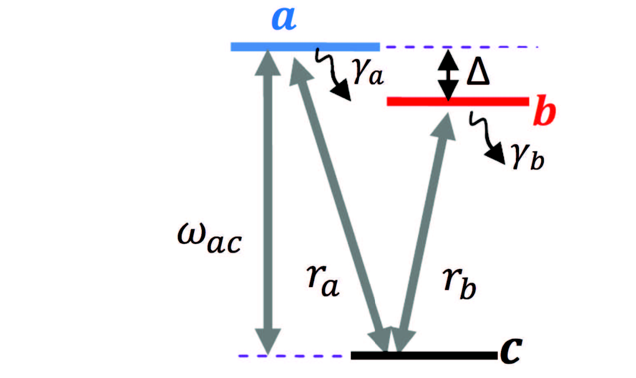
The three-level V-system comprising a single ground state coupled by the system-bath interaction to a pair of excited states (see Fig. 1) serves as a minimal model of a multilevel quantum system exhibiting non-trivial Fano coherence dynamics. This system has been extensively studied in the weak-pumping limit (relevant for photosynthetic light-harvesting) where incoherent excitation occurs much more slowly than spontaneous emission. In this limit, the coherent dynamics of the V-system is determined by the ratio ζ=12​(γa+γb)/Δp\zeta=\frac{1}{2}(\gamma_{a}+\gamma_{b})/\Delta_{p}, where Δp=Δ2+(1−p2)​γa​γb\Delta_{p}=\sqrt{\Delta^{2}+(1-p^{2})\gamma_{a}\gamma_{b}} is the renormalized excited-level splitting, γa\gamma_{a} and γb\gamma_{b} are the spontaneous decay rates, and pp is the angle between the transition dipole moments of the g→ag\to a and g→bg\to b transitions (see Fig. 1) [14]. The two-photon coherences between the excited states of the V-system exhibit damped oscillations in the regime where the excited levels are widely spaced (ζ≪1\zeta\ll 1). In the opposite regime of small level spacing (ζ≫1\zeta\gg 1), the coherences evolve monotonously and can survive for an arbitrarily long time τc=2​γa​γb/Δp2\tau_{c}=2\sqrt{\gamma_{a}\gamma_{b}}/\Delta_{p}^{2} [13, 14].

While the weak pumping regime of noise-induced coherent dynamics is well understood [9, 13, 14, 15], much less is known about the opposite limit where incoherent excitation occurs much faster than spontaneous emission. The strong pumping regime is central to the theory of quantum heat engines, where quantum coherence has been predicted to enhance the engine’s efficiency [11, 12]. Accordingly, the generation and steady-state properties of quantum coherences in this regime have been studied in closed-cycle quantum heat engine models [11] and in the degenerate Λ\Lambda-system [10]. However, these studies did not explore the time dynamics of the coherences as a function of the system’s excited-state splitting and radiative decay rates. In addition, the quantum heat engine studies [11, 12] considered a more complex case of a 5-level system interacting with two baths, where the coherences emerge as a result of non-equilibrium transport dynamics involving both of the baths. This leaves open the question of whether strong incoherent driving can generate coherences in multilevel quantum systems interacting with a single thermal bath.

Here, we address this question by presenting a theoretical analysis of the quantum dynamics of a V-system strongly driven by a thermal bath. We derive closed-form analytic solutions of the Bloch-Redfield (BR) quantum master equations, which show that (1) quantum coherences can be generated by strong incoherent driving provided that the transition dipole moments of the V-system are nearly perfectly aligned, and (2) the coherence lifetime scales linearly with the pumping intensity n¯\bar{n} and quadratically with the inverse excited-level spacing γ/Δ\gamma/\Delta. These results suggest the possibility of observing long-lived coherence dynamics in strongly driven Rydberg atoms and polyatomic molecules.

This paper is structured as follows. In Sec. II we present the theoretical formalism based on the BR master equations and outline the procedure of their analytical solution. The dynamical regimes of the strongly driven V-system are classified in Sec. IIB. Sections IIC and III present analytical expressions for the coherence lifetimes and for the time dynamics of the populations and coherences. Section IV summarizes the main fundings of this work and outlines an experimental scenario for observing the noise-induced coherences.

II Theory

II.1 Bloch-Redfield equations and their general solution

Consider a three-level V-system weakly coupled to a thermal environment (see Fig. 1). The system resides in the ground state |a⟩|a\rangle (i.e. ρa​a​(0)=1\rho_{aa}(0)=1) before the system-environment coupling is suddenly turned on at t=0t=0, leading to the population transfer to the excited states |b⟩|b\rangle and |c⟩|c\rangle. To describe the time evolution of the system, we use a quantum master equation approach based on the Liouville-von Neumann equation for the density operator of the system+bath complex [2, 21, 1]. Neglecting the system-bath correlations, tracing over the bath modes, and adopting the Markov approximation for bath correlation functions, we arrive at the Bloch-Redfield (BR) master equation for the reduced density matrix of the V-system [8, 9, 13, 14]

ρ˙i​i\displaystyle\dot{\rho}_{ii} =−(ri+γi)​ρi​i+ri​ρc​c−p⁡(ra​rb+γa​γb)​ρa​bR\displaystyle=-(\textit{r}_{i}+\gamma_{i})\rho_{ii}+\textit{r}_{i}\rho_{cc}-p(\sqrt{\textit{r}_{a}\textit{r}_{b}}+\sqrt{\gamma_{a}\gamma_{b}})\rho^{R}_{ab} (1)
ρ˙a​b\displaystyle\dot{\rho}_{ab} =−12​(ra+rb+γa+γb)​ρa​b−i​ρa​b​Δ\displaystyle=-\frac{1}{2}(\textit{r}_{a}+\textit{r}_{b}+\gamma_{a}+\gamma_{b})\rho_{ab}-i\rho_{ab}\Delta
+p2​ra​rb​(2​ρc​c−ρa​a−ρb​b)−p2​γa​γb​(ρa​a+ρb​b)\displaystyle+\frac{p}{2}\sqrt{\textit{r}_{a}\textit{r}_{b}}(2\rho_{cc}-\rho_{aa}-\rho_{bb})-\frac{p}{2}\sqrt{\gamma_{a}\gamma_{b}}(\rho_{aa}+\rho_{bb}) (2)

where aa, bb, and cc are the system’s energy eigenstates, the two-photon coherence ρa​b=ρa​bR+i​ρa​bI\rho_{ab}=\rho^{R}_{ab}+i\rho^{I}_{ab} is given as a sum of its real and imaginary parts, and we have used the conservation of probability condition to express ρa​a=1−ρb​b−ρc​c\rho_{aa}=1-\rho_{bb}-\rho_{cc}.

The BR equations are parametrized by the excited-state energy splitting Δ=ωa​b\Delta=\omega_{ab} (see Fig. 1), the system-bath coupling parameters γi\gamma_{i} (i=a,bi=a,b) which determine the rate of spontaneous decay into the vacuum modes of the bath, and the (pseudo)thermal pumping rates ri=γi​n¯r_{i}=\gamma_{i}\bar{n} [16], where n¯\bar{n} is the effective occupation number of thermal modes at the transition frequency ωa​c\omega_{ac} (see Fig. 1). In thermal equilibrium, n¯=(1−eβ​ω0)−1\bar{n}=(1-e^{\beta\omega_{0}})^{-1}, where β=1/kB​T\beta=1/k_{B}T, TT is the temperature of the bath, and kBk_{B} is Boltzmann’s constant. An important parameter p=μ→a​c.μ→b​c|μ→a​c|​|μ→b​c|p=\frac{\vec{\mu}_{ac}.\vec{\mu}_{bc}}{|\vec{\mu}_{ac}||\vec{\mu}_{bc}|} quantifies the alignment of the transition dipole moment vectors μ→a​c\vec{\mu}_{ac} and μ→b​c\vec{\mu}_{bc} [8, 9, 13, 14]. We will show that the solutions of the BR equations tend to be extremely sensitive to the value of pp. Note that for p=0p=0, the BR equations reduce to the standard Pauli rate equations, which give coherence-free dynamics [8, 9, 13, 14], We will therefore focus on the non-trivial case of p≠0p\neq 0.

The BR quantum master equations (1) generally describe the dynamics of the V-system interacting with stochastic bosonic fields, such as photons or phonons [2]. Here, we will consider the BR equations in a quantum optical context, relevant to the incoherent light excitation of quantum heat engines in the strong pumping limit, n¯≫1\bar{n}\gg 1. We can then identify γi=ωc​i3​|μ→c​i|23​π​ϵ0​ℏ​c3\gamma_{i}=\frac{\omega_{ci}^{3}|\vec{\mu}_{ci}|^{2}}{3\pi\epsilon_{0}\hbar c^{3}} with the spontaneous emission rate of the excited level i=a,bi=a,b. Further, ri=Bi​W​(ωc​i)\textit{r}_{i}=B_{i}W(\omega_{ci}) are the incoherent pumping rates of |c⟩\ket{c} ↔\leftrightarrow |i⟩\ket{i} transitions with Bi=π​|μ→c​i|23​ϵ0​ℏ2B_{i}=\frac{\pi|\vec{\mu}_{ci}|^{2}}{3\epsilon_{0}\hbar^{2}} being the Einstein’s BB-coefficients and W⁡(ωc​i)W(\omega_{ci}) is the intensity of the incident blackbody radiation at the corresponding transition frequencies. Finally, ri=n¯​γir_{i}=\bar{n}\gamma_{i} are the incoherent absorption rates defined in terms of the effective photon occupation number n¯=Bi​W​(ωc​i)/γi\bar{n}=B_{i}W(\omega_{ci})/\gamma_{i} [9, 13, 16], which is proportional to the pumping intensity.

A comment is in order regarding the validity of the BR quantum mater equations in the strong-pumping limit. The weak-coupling assumption underlying the BR equations holds as long as the system-bath coupling (as quantified by the incoherent pumping rates rr) is much smaller than the energy gap ωa​c\omega_{ac} between the ground and excited energy eigenstates (see Fig. 1). This condition is well satisfied for typical optical frequencies (ωa​c∼106\omega_{ac}\sim 10^{6} GHz [2]) and incoherent pumping rates (ri=1−103r_{i}=1-10^{3} GHz) corresponding to the effective photon occupation numbers n¯=10−103\bar{n}=10-10^{3} typically used in few-level models of quantum heat engines [19, 20, 11, 12]. Thus, the strong-pumping condition r≫γr\gg\gamma remains valid in the weak-coupling limit. In contrast, the Markovian assumption is expected to break down at very large pumping rates approaching the inverse bath correlation times 1/τc1/\tau_{c}. In this limit, the BR equations remain valid as long as ri≪1/τcr_{i}\ll 1/\tau_{c}. For incoherent pumping with solar light (τc∼1.3\tau_{c}\sim 1.3 fs), this condition implies n¯≪1/(τc​γi)≃106\bar{n}\ll 1/(\tau_{c}\gamma_{i})\simeq 10^{6}, which is much larger than the effective photon occupation numbers considered here (n¯=102−103\bar{n}=10^{2}-10^{3}). Following previous theoretical work [11, 12, 19, 20], we neglect multiphoton transitions originating from the excited states of the V-system.

Here we consider the case of a symmetric V-system, where γa=γb=γ\gamma_{a}=\gamma_{b}=\gamma, ra=rb=r\textit{r}_{a}=\textit{r}_{b}=\textit{r}, and hence ρa​a​(t)=ρb​b​(t)\rho_{aa}(t)=\rho_{bb}(t) [13]. The imposed symmetry simplifies the analytical solution of the BR equations to a great extent, while retaining the essential features of the dynamics [13, 14]. The BR master equations for the symmetric V-system (1) can be expressed in matrix-vector form

𝒙˙​(t)=𝐀​𝒙​(t)+𝒅,\dot{\bm{x}}(t)=\mathbf{A}\bm{x}(t)+\bm{d}, (3)

where 𝒙⁡(t)=[ρa​a​(t),ρa​bR​(t),ρa​bI​(t)]T{\bm{x}}(t)=[\rho_{aa}(t),\rho_{ab}^{R}(t),\rho_{ab}^{I}(t)]^{T} is the state vector in the Liouville representation, where the elements of a N×NN\times N density matrix are represented by a vector of dimension N2N^{2} [21], and 𝒅=[r,p​r,0]T\bm{d}=[r,p{r},0]^{T} is the driving vector. Note that the state vector excludes the ground-state population and the one-photon coherences ρa​c\rho_{ac} and ρb​c\rho_{bc}, which evolve independently [8]. The coefficient matrix 𝐀\mathbf{A} in Eq. (3) is given by

𝐀=[−(3​r+γ)−p⁡(r+γ)0−p⁡(3​r+γ)−(r+γ)Δ0−Δ−(r+γ)].\mathbf{A}=\begin{bmatrix}-(3\textit{r}+\gamma)&-p(\textit{r}+\gamma)&0\\ -p(3\textit{r}+\gamma)&-(\textit{r}+\gamma)&\Delta\\ 0&-\Delta&-(\textit{r}+\gamma)\\ \end{bmatrix}. (4)

The general solution of the system of inhomogeneous differential equations (3) may be obtained as [23]

𝒙⁡(t)=e𝐀​t​𝒙0+∫0td​s​e𝐀⁡(t−s)​𝒅​(s),\bm{x}{(t)}=e^{\mathbf{A}t}\bm{x}_{0}+\int_{0}^{t}dse^{\mathbf{A}(t-s)}\bm{d}(s), (5)

where 𝒙0\bm{x}_{0} specifies the initial conditions for the density matrix, and 𝒅⁡(s)\bm{d}(s) is the driving vector defined above. Since our interest here is in the generation of noise-induced Fano coherences by incoherent driving, we choose a coherence-free initial state ρc​c​(t=0)=1\rho_{cc}(t=0)=1, or 𝒙0=(0,0,0)T\bm{x}_{0}=(0,0,0)^{T}, corresponding to the V-system initially in the ground state. The exponent of matrix 𝐀\mathbf{A} in Eq. (5) and the density matrix dynamics 𝒙⁡(t)\bm{x}{(t)} can be evaluated analytically in the limit n¯≫1\bar{n}\gg 1 by expanding the matrix elements in the small parameter x=1/n¯x=1/\bar{n} as described in the Appendix.

II.2 Dynamical regimes

The behavior of the general solution of the BR equations (5) is determined by the eigenvalue spectrum λk\lambda_{k} of the coefficient matrix 𝐀\mathbf{A}. While the spectrum can be obtained analytically as described below and in the Appendix, its general features can be understood by examining the discriminant DD of the characteristic equation for 𝐀\mathbf{A}

D=B3+[C−32​A​(B+A2)]2,D=B^{3}+\left[C-\frac{3}{2}A(B+A^{2})\right]^{2}, (6)

where

A\displaystyle A =13​(5​r+3​γ),\displaystyle=\frac{1}{3}(5r+3\gamma),
B\displaystyle B =13​(r+γ)​[Δ2+(r+γ)+(2−p2)​(3​r+γ)]−A2,\displaystyle=\frac{1}{3}(r+\gamma)[\Delta^{2}+(r+\gamma)+(2-p^{2})(3r+\gamma)]-A^{2},
C\displaystyle C =12​(3​r+γ)​[Δ2+(1−p2)​(r+γ)2]+A3\displaystyle=\frac{1}{2}(3r+\gamma)[\Delta^{2}+(1-p^{2})(r+\gamma)^{2}]+A^{3} (7)

The above expressions are valid for all pp.

Depending on the sign of DD, three dynamical regimes can be distinguished:

  1. 1.

    Underdamped regime (D>0D>0). If the discriminant (6) is positive, one of the eigenvalues of 𝐀\mathbf{A} is real and the other two eigenvalues are complex. The corresponding normal modes include an exponentially decaying eigenmode and two oscillating eigenmodes. Using the analogy with the damped harmonic oscillator [14], we will refer to this regime as underdamped.

  2. 2.

    Overdamped regime (D<0D<0). If the discriminant (6) is negative, all of the eigenvalues λk\lambda_{k} are real with Re​(λk)<0\text{Re}(\lambda_{k})<0, and thus all normal modes decay exponentially. Following our previous work [14], we will refer to this regime as overdamped.

  3. 3.

    Critical regime (D=0D=0). If the discriminant (6) vanishes, all of the eigenvalues λk\lambda_{k} are real with at least two of them being equal. This is the critical regime [14], which marks a transition between the underdamped and overdamped regimes.

To classify the dynamical regimes of the strongly driven V-system, we therefore need to identify the regions of the parameter space where the discriminant (6) takes on positive and negative values. As shown in the Appendix, the discriminant can be expressed as a polynomial function of the occupation number n¯=r/γ\bar{n}={r}/{\gamma}

D=γ6108​∑k=06dk​n¯kD=\frac{\gamma^{6}}{108}\sum\limits_{k=0}^{6}d_{k}\bar{n}^{k} (8)

where the coefficients dkd_{k} depend on the ratio Δ/γ\Delta/\gamma of the excited-state splitting to the radiative decay rate and the transition dipole alignment factor pp.

Figure 2 shows the lines of zero discriminant separating the overdamped (D>0D>0) from underdamped (D<0D<0) regimes as a function of the average photon occupation number n¯\bar{n} and the excited-state energy splitting Δ/γ\Delta/\gamma for selected values of pp. A contour plot of the discriminant is shown in Fig. 3. We observe that when both n¯\bar{n} and Δ/γ\Delta/\gamma are large, the solution of the equation D=0D=0 is given by the straight line Δ/γ=f⁡(p)​n¯\Delta/\gamma=f(p)\bar{n}. It can be shown analytically (see the Appendix) that the slope of the line f⁡(p)f(p) is a function of pp only. The slope function f⁡(p)f(p) plotted in Fig. 4(a) increases monotonically from zero to 0.6 as pp is varied between 0 and 1.

As illustrated in Fig. 3(a), the discriminant is positive in the underdamped region above the zero-DD lines, where the coherences exhibit damped oscillations. Below the D=0D=0 lines, the sign of DD changes from positive to negative and the V-system enters the overdamped regime, with coherences evolving monotonously as a function of time. Since, as shown above, the zero-DD lines are described by Δ/γ=f⁡(p)​n¯\Delta/\gamma=f(p)\bar{n} at large n¯\bar{n} and Δ/γ\Delta/\gamma, the dynamical regimes of the strongly driven V-system can be classified based on a single dimensionless parameter Δ/(n¯​γ)=Δ/r\Delta/(\bar{n}\gamma)=\Delta/r. The overdamped regime is defined by the condition Δ/(n¯​γ)<f⁡(p)\Delta/(\bar{n}\gamma)<f(p) whereas the underdamped regime is defined by Δ/(n¯​γ)>f⁡(p)\Delta/(\bar{n}\gamma)>f(p). For perfectly aligned transition dipole moments, we have f⁡(1)=0.6f(1)=0.6 [see Fig. 4(a)] and the overdamped regime occurs for Δ/(n¯​γ)<0.6\Delta/(\bar{n}\gamma)<0.6. As the transition dipoles get out of alignment, the function f⁡(p)f(p) decreases, and smaller values of Δ\Delta are needed to reach the overdamped regime for a given n¯\bar{n}. For instance, at p=1/2p=1/2 the overdamped regime is reached for Δ/(n¯​γ)<0.16\Delta/(\bar{n}\gamma)<0.16 as illustrated in Fig. 2(a), which shows that the slopes of the D=0D=0 lines decrease proportionally to pp.

Figures 2(a) and 2(b) show that the overdamped regime becomes progressively more widespread with increasing the pumping intensity n¯\bar{n}. For large values of p≃1p\simeq 1 and n¯≫10\bar{n}\gg 10 of interest here, the underdamped regime is reached only at very large excited-state splittings (Δ/γ≫10\Delta/\gamma\gg 10). In contrast, incoherent excitation of large molecules with dense spectra of rovibrational levels [13] and quantum heat engines [11, 12] typically occurs in the small level spacing regime Δ/γ≪1\Delta/\gamma\ll 1. This is the regime we will consider in the remainder of this paper.

As shown in Figs. 2(b), the zero-DD lines approach constant values Δ/p​γ\Delta/p\gamma in the weak pumping limit (n¯→0\bar{n}\to 0). This implies that in this limit, the boundary between the overdamped and underdamped dynamical regimes is defined by the condition Δ/p​γ=1\Delta/p\gamma=1, which is consistent with our previous results [13, 14]. It worth observing that the zero-DD lines in Fig. 2(b) curve downward as n¯\bar{n} increases from zero to n¯∼0.01\bar{n}\sim 0.01. The reason for this is that the linear term (d1​n¯d_{1}\bar{n}) in Eq. (8) becomes negligible compared to the zeroth and second-order terms and the discriminant is given by D=γ6108​(d0+d2​n¯2)D=\frac{\gamma^{6}}{108}(d_{0}+d_{2}\bar{n}^{2}). At higher values of n¯∼0.1\bar{n}\sim 0.1, the zero-DD lines reach a minimum and then start to approach their large-n¯\bar{n} limiting values as discussed above.

II.3 Eigenvalues and coherence lifetimes

As discussed in Sec. IIA, in order to obtain the general solution of the BR equations (5), it is necessary to find the exponent of the coefficient matrix 𝐀\mathbf{A}. To this end, we first diagonalize 𝐀\mathbf{A} to obtain the eigenvalues λk\lambda_{k}, which give the inverse lifetimes (or decay rates) of the corresponding normal modes 𝑽k\bm{V}_{k} [13, 14]. Expanding the characteristic equation for 𝐀\mathbf{A} in terms of the small parameter x=γ/r=1/n¯x={\gamma}/{r}={1}/{\bar{n}} (see the Appendix) we obtain the eigenvalues as

λj=r​∑k=08zj​k​xk,(j=1,2,3).\lambda_{j}=r\sum_{k=0}^{8}z_{jk}x^{k},\quad(j=1,2,3). (9)

This expansion (9) is valid for x≤0.01x\leq 0.01 and p>0.1p>0.1 (for Δ/γ<1\Delta/\gamma<1) and 0.89<p<10.89<p<1 (for Δ/γ>1\Delta/\gamma>1).

In the overdamped regime, where Δγ​n¯≪f⁡(p)\frac{\Delta}{\gamma\bar{n}}\ll f(p), the expansion (9) converges rapidly. Keeping the lowest-order terms, we find to excellent accuracy

λj=r⁡[zj​0+zj​1​x+zj​2​x2],\lambda_{j}=r[z_{j0}+z_{j1}x+z_{j2}x^{2}], (10)

where the expressions for the coefficients zj​kz_{jk} in terms of the system parameters pp, Δ/γ\Delta/\gamma, and n¯\bar{n} are (see the Appendix)

zj​0​(p)\displaystyle z_{j0}(p) =(8+27​p2)27+p4​(1+3​p2)3​i3\displaystyle=\sqrt[3]{\frac{(8+27p^{2})}{27}+\sqrt{\frac{p^{4}(1+3p^{2})}{3}}i}
zj​1​(p)\displaystyle z_{j1}(p) =−1−αj3​K​4​p2+[αj3​K​(43+3​p2)−βj​K]​v1,\displaystyle=-1-\frac{\alpha_{j}}{3K}4p^{2}+\left[\frac{\alpha_{j}}{3K}\left(\frac{4}{3}+3p^{2}\right)-\beta_{j}K\right]v_{1},
zj​2​(p)\displaystyle z_{j2}(p) =fj​1​(p)​(Δγ)2+fj​2​(p),\displaystyle=f_{j1}(p)\left(\frac{\Delta}{\gamma}\right)^{2}+f_{j2}(p), (11)

and the parameters KK, v1v_{1} and fj​k​(p)f_{jk}(p) are listed in Tables 1, 2, and 4 of the Appendix. Here αj\alpha_{j} and βj\beta_{j} are the cube roots of unity with values (α1,β1)=(1,1)(\alpha_{1},\beta_{1})=(1,1), (α2,β2)=(ω2,ω)(\alpha_{2},\beta_{2})=(\omega^{2},\omega), (α3,β3)=(ω,ω2)(\alpha_{3},\beta_{3})=(\omega,\omega^{2}) with ω=(−1+i​3)2\omega=\frac{(-1+i\sqrt{3})}{2} and ω2=(−1−i​3)2\omega^{2}=\frac{(-1-i\sqrt{3})}{2}. Note that since these parameters depend on pp only, the coefficients zj​1z_{j1} and zj​0z_{j0} are independent of the ratio of the excited-state splitting to the radiative decay rate Δ/γ{\Delta}/{\gamma}. In contrast, the coefficient of x2x^{2} in Eq. (10) carries an explicit quadratic dependence on Δ/γ\Delta/\gamma.

In order to compare the relative importance of the different terms in Eq. (10), we plot in Fig. 5 the pp dependence of ln⁡|zj​k|\ln|z_{jk}| for k=0k=0 - 2. Figures 5(a) and 5(c) show that z10z_{10} provides the dominant contribution to λ1\lambda_{1} and z30z_{30} provides the dominant contribution to λ3\lambda_{3} for all pp, and we can thus approximate

λj=r​zj​0=(γ​zj​0)​n¯,(j=1,3)\lambda_{j}=rz_{j0}=(\gamma z_{j0})\bar{n},\kern 5.0pt(j=1,3) (12)

where zj​0​(p)z_{j0}(p) are given by Eq. (11). The scaling behavior given by Eq. (12) is illustrated in Fig. 6(b), which shows that the eigenvalues λ1\lambda_{1} and λ3\lambda_{3} are independent of Δ/γ{\Delta}/{\gamma} regardless of the value of pp.

Remarkably, however, this is not the case for the eigenvalue λ2\lambda_{2}: As shown in Fig. 5(b) there is a critical value of p=pcp=p_{c} at which the curves z20​(p)z_{20}(p) and z22​(p)​x2z_{22}(p)x^{2} cross and the relative contributions of the different terms to λ2\lambda_{2} change dramatically. At p<pcp<p_{c}, z20​(p)z_{20}(p) is the dominating term so λ2\lambda_{2} scales in the same way as the other eigenvalues (12). For p>pcp>p_{c}, the leading term is z22​x2z_{22}x^{2} and hence the scaling of λ2\lambda_{2} with Δ/γ\Delta/\gamma is, quadratic the same as that of z22z_{22} [see Eq. (11)]. The critical value of pp depends on Δ/γ\Delta/\gamma and n¯\bar{n} and ranges from 0.995 to 1.0 for n¯=103\bar{n}=10^{3} and Δ/γ=102−10−2\Delta/\gamma=10^{2}-10^{-2} [See Fig. 4(b)]. The remarkable sensitivity of the second eigenvalue to the transition dipole alignment parameter pp shown in Fig. 5(c) leads to qualitatively different population and coherence dynamics for p<pcp<p_{c} and p>pcp>p_{c} as shown below.

As shown in Fig. 5(b), the quadratic contribution to the second eigenvalue is much larger than the linear and constant terms, and hence λ2≃r​zj​2​(γ/r)2\lambda_{2}\simeq rz_{j2}({\gamma}/{r})^{2}. Combining Eqs. (10) and (11) and noting that f22​(p)→0f_{22}(p)\rightarrow 0 for p>pcp>p_{c}, we find

λ2=γn¯​f21​(p)​(Δγ)2\lambda_{2}=\frac{\gamma}{\bar{n}}f_{21}(p)\left(\frac{\Delta}{\gamma}\right)^{2} (13)

The distinct quadratic scaling of λ2\lambda_{2} with Δ/γ\Delta/\gamma is illustrated in Fig. 6(a). The function f21​(p)f_{21}(p) (see the Appendix) increases monotonously approaching the value −0.749-0.749 in the limit p→1p\to 1. As the second eigenvalue gives the decay rate of the real part of the coherence (see Sec. IIA) the coherence lifetime τc=1/|λ2|\tau_{c}=1/|\lambda_{2}| is given by

τc=1.34​n¯γ​(Δγ)−2(p>pc).\tau_{c}=1.34\frac{\bar{n}}{\gamma}\left(\frac{\Delta}{\gamma}\right)^{-2}\qquad(p>p_{c}). (14)

The linear scaling of the coherence lifetime with the incoherent pumping intensity n¯\bar{n} is a direct consequence of the second eigenvalue being dominated by a single z22​x2z_{22}x^{2} contribution as shown in Fig. 5(b). This characteristic scaling occurs only for p>pcp>p_{c} with pc=1−ϵp_{c}=1-\epsilon very close to unity [typical values of ϵ\epsilon range from 5×10−115\times 10^{-11} to 5×10⁻³⁵\times 10^{-3} for n¯=103\bar{n}=10^{3} as shown in Fig. 4(b). Thus, the V-system with nearly parallel transition dipole moments can exhibit very long coherence times in the strong pumping limit.

For subcritical transition dipole alignment (p<pcp<p_{c}), the coherence lifetime becomes

τc=1γ​z20​(p)​n¯−1(p<pc).\tau_{c}=\frac{1}{\gamma z_{20}(p)}\bar{n}^{-1}\qquad(p<p_{c}). (15)

The coherence lifetimes thus become shorter with increasing the pumping intensity, in stark contrast with the situation in the supercritical regime (p>pcp>p_{c}), where the lifetimes increase linearly with n¯\bar{n} (14).

It is instructive to compare the coherence time of the V-system in the strong-pumping and weak-pumping regimes. In the small level spacing regime (Δ/γ<1\Delta/\gamma<1), the coherence time under weak pumping τcW​P=2γ​(Δγ)−2\tau_{c}^{WP}=\frac{2}{\gamma}\left(\frac{\Delta}{\gamma}\right)^{-2} [13, 14] exhibits the same (Δ/γ)−2(\Delta/\gamma)^{-2} scaling as in the strong-pumping regime [13, 14], becoming longer as the excited-state energy gap Δ\Delta narrows down. The ratio of the coherence times in the strong and weak-pumping limits is thus, for p>pcp>p_{c}

τcτcW​P≃0.67​n¯\frac{\tau_{c}}{\tau_{c}^{WP}}\simeq 0.67\bar{n} (16)

The enhancement of the coherence lifetime under strong pumping (n>1.5n>1.5) may facilitate the experimental observation of the noise-induced coherences in atomic systems [22].

We note in passing that nearly perfect alignment of the transition dipole moments (p>pcp>p_{c}) is an essential condition for the longevity of noise-induced coherences in the strong pumping regime. In practice, since pcp_{c} is very close to unity, this condition is equivalent to the requirement p=1p=1. The coherence lifetime exhibits two dramatically different scalings with the pumping intensity n¯\bar{n}. For p<pcp<p_{c}, the lifetime decreases with n¯\bar{n}, whereas for p>pcp>p_{c} the opposite trend is observed. This means that in the strong-pumping limit, even slightest misalignment of the transition dipole moments will destroy long-lived coherent dynamics.

III Population and coherence dynamics

III.1 Analytic solutions in the overdamped regime [Δ/(n¯​γ)<f⁡(p)\Delta/(\bar{n}\gamma)<f(p)]

Having classified the dynamical regimes of the strongly driven V-system and analyzed the relevant eigenmodes, we now turn to the time evolution of the density matrix elements. From Eq. (5), we obtain [24]

ρi​j​(t)=rdet⁡(𝐌)​∑k=13(eλk​t−1)λk​Vk,n⁡(i,j)​(Tk​1+p​Tk​2).\rho_{ij}(t)=\frac{r}{\det(\mathbf{M})}\sum_{k=1}^{3}\frac{(e^{\lambda_{k}t}-1)}{\lambda_{k}}V_{k,n(i,j)}(T_{k1}+pT_{k2}). (17)

where n⁡(i,j)n(i,j) = 1 for the excited-state population (i=j=ai=j=a) and n​(i,j)=2​(3)n(i,j)=2(3) for the real (imaginary) part of the two-photon coherence (i=a,j=bi=a,j=b). The density matrix elements in Eq. (17) are expressed as a linear combination of exponentially decaying terms, weighted with the components Vk​jV_{kj} of eigenvectors of 𝐀\mathbf{A} (which form the fundamental matrix 𝐌\mathbf{M}) and the elements of its adjoint matrix Tk​jT_{kj}, which depend on pp only.

To express the density matrix dynamics in terms of the physical parameters Δ/γ\Delta/\gamma, n¯\bar{n}, and pp, we evaluate the eigenvector components Vk​jV_{kj} and Tk​jT_{kj} in Eq. (17) as described in the Appendix and use the resulting expressions in Eq. (5) to obtain for p>pcp>p_{c}

ρa​a​(t)=1[T1​(p)+T2​(p)​1n¯2​(Δγ)2]{[A1+A21n¯2(Δγ)2]1−e−γ​|z10​(p)|​n¯​t|z10​(p)|+[A3+A41n¯2(Δγ)2]n¯2(Δγ)−21−e−γ​|f21​(p)|​1n¯​(Δγ)2​t|f21​(p)|+A51n¯2(Δγ)21−e−γ​|z30​(p)|​n¯​t|z30​(p)|}\begin{split}\rho_{aa}(t)&=\frac{1}{[T_{1}(p)+T_{2}(p)\frac{1}{\bar{n}^{2}}(\frac{\Delta}{\gamma})^{2}]}\biggl\{\left[A_{1}+A_{2}\frac{1}{\bar{n}^{2}}\left(\frac{\Delta}{\gamma}\right)^{2}\right]\frac{1-e^{-\gamma|z_{10}(p)|\bar{n}t}}{|z_{10}(p)|}\\ &+\left[A_{3}+A_{4}\frac{1}{\bar{n}^{2}}\left(\frac{\Delta}{\gamma}\right)^{2}\right]\bar{n}^{2}\left(\frac{\Delta}{\gamma}\right)^{-2}\frac{1-e^{-\gamma|f_{21}(p)|\frac{1}{\bar{n}}(\frac{\Delta}{\gamma})^{2}t}}{|f_{21}(p)|}+A_{5}\frac{1}{\bar{n}^{2}}\left(\frac{\Delta}{\gamma}\right)^{2}\frac{1-e^{-\gamma|z_{30}(p)|\bar{n}t}}{|z_{30}(p)|}\biggr\}\end{split} (18)
ρa​bR​(t)=1[T1​(p)+T2​(p)​1n¯2​(Δγ)2]{[B1+B21n¯2(Δγ)2]1−e−γ​|z10​(p)|​n¯​t|z10​(p)|+[B3+B41n¯2(Δγ)2]n¯2(Δγ)−21−e−γ​|f21​(p)|​1n¯​(Δγ)2​t|f21​(p)|+B51n¯2(Δγ)21−e−γ​|z30​(p)|​n¯​t|z30​(p)|}\begin{split}\rho^{R}_{ab}(t)&=\frac{1}{[T_{1}(p)+T_{2}(p)\frac{1}{\bar{n}^{2}}(\frac{\Delta}{\gamma})^{2}]}\biggl\{\left[B_{1}+B_{2}\frac{1}{\bar{n}^{2}}\left(\frac{\Delta}{\gamma}\right)^{2}\right]\frac{1-e^{-\gamma|z_{10}(p)|\bar{n}t}}{|z_{10}(p)|}\\ &+\left[B_{3}+B_{4}\frac{1}{\bar{n}^{2}}\left(\frac{\Delta}{\gamma}\right)^{2}\right]\bar{n}^{2}\left(\frac{\Delta}{\gamma}\right)^{-2}\frac{1-e^{-\gamma|f_{21}(p)|\frac{1}{\bar{n}}(\frac{\Delta}{\gamma})^{2}t}}{|f_{21}(p)|}+B_{5}\frac{1}{\bar{n}^{2}}\left(\frac{\Delta}{\gamma}\right)^{2}\frac{1-e^{-\gamma|z_{30}(p)|\bar{n}t}}{|z_{30}(p)|}\biggr\}\end{split} (19)
ρa​bI​(t)=1[T1​(p)+T2​(p)​1n¯2​(Δγ)2]1n¯(Δγ){[C1+C21n¯2(Δγ)2]1−e−γ​|z10​(p)|​n¯​t|z10|+[C3+C41n¯2(Δγ)2]n¯2(Δγ)−21−e−γ​|f21​(p)|​1n¯​(Δγ)2​t|f21​(p)|+[C5+C61n¯2(Δγ)2]1−e−γ​|z30|​n¯​t|z30​(p)|},\begin{split}\rho^{I}_{ab}(t)&=\frac{1}{[T_{1}(p)+T_{2}(p)\frac{1}{\bar{n}^{2}}(\frac{\Delta}{\gamma})^{2}]}\frac{1}{\bar{n}}\left(\frac{\Delta}{\gamma}\right)\biggl\{\left[C_{1}+C_{2}\frac{1}{\bar{n}^{2}}\left(\frac{\Delta}{\gamma}\right)^{2}\right]\frac{1-e^{-\gamma|z_{10}(p)|\bar{n}t}}{|z_{10}|}\\ &+\left[C_{3}+C_{4}\frac{1}{\bar{n}^{2}}\left(\frac{\Delta}{\gamma}\right)^{2}\right]\bar{n}^{2}\left(\frac{\Delta}{\gamma}\right)^{-2}\frac{1-e^{-\gamma|f_{21}(p)|\frac{1}{\bar{n}}(\frac{\Delta}{\gamma})^{2}t}}{|f_{21}(p)|}+\left[C_{5}+C_{6}\frac{1}{\bar{n}^{2}}\left(\frac{\Delta}{\gamma}\right)^{2}\right]\frac{1-e^{-\gamma|z_{30}|\bar{n}t}}{|z_{30}(p)|}\biggr\},\end{split} (20)

where the eigenvalue components zj​0​(p)z_{j0}(p) are given by Eqs. (11) and the coefficients AiA_{i}, BiB_{i}, and CiC_{i} plotted in Figs. 7 and 8 depend on pp only (see the Appendix for analytic expressions, which are rather cumbersome). The second term on the right-hand-side of Eq. (19) represents the slowly decaying coherent mode discussed in Sec. IIB, which also manifests itself in the time evolution of excited-state populations (18). The lifetime of the coherent mode scales as n¯​(Δ/γ)−2\bar{n}(\Delta/\gamma)^{-2}, leading to arbitrarily long coherence lifetimes for small excited-state splittings. In contrast, the first and third terms on the right-hand side of Eqs. (18)-(20) decay much faster, with lifetimes proportional to 1/n¯1/\bar{n}.

To further simplify our analytic solutions (18)-(20), we note that the coefficients AiA_{i}, BiB_{i}, and CiC_{i} plotted in Figs. 7 and 8 do not vary strongly with pp in the vicinity of p=1p=1. We can thus replace the coefficients by their limiting values at p→1p\to 1 to yield

ρa​a​(t)=1[−4+1.33​1n¯2​(Δγ)2]{[−4+2.921n¯2(Δγ)2](1−e−4​γ​n¯​t)4−(1−e−0.75​γn¯​(Δγ)2​t)3+0.441n¯2(Δγ)2(1−e−γ​n¯​t)}\begin{split}\rho_{aa}(t)&=\frac{1}{[-4+1.33\frac{1}{\bar{n}^{2}}(\frac{\Delta}{\gamma})^{2}]}\biggl\{\left[-4+2.92\frac{1}{\bar{n}^{2}}\left(\frac{\Delta}{\gamma}\right)^{2}\right]\frac{(1-e^{-4\gamma\bar{n}t})}{4}\\ &-\frac{(1-e^{-0.75\frac{\gamma}{\bar{n}}(\frac{\Delta}{\gamma})^{2}t})}{3}+0.44\frac{1}{\bar{n}^{2}}\left(\frac{\Delta}{\gamma}\right)^{2}(1-e^{-\gamma\bar{n}t})\biggr\}\end{split} (21)
ρa​bR​(t)=1[−4+1.33​1n¯2​(Δγ)2]{[−4+3.2491n¯2(Δγ)2](1−e−4​γ​n¯​t)4+(1−e−0.75​γn¯​(Δγ)2​t)−0.891n¯2(Δγ)2(1−e−γ​n¯​t)}\begin{split}\rho^{R}_{ab}(t)&=\frac{1}{[-4+1.33\frac{1}{\bar{n}^{2}}(\frac{\Delta}{\gamma})^{2}]}\biggl\{\left[-4+3.249\frac{1}{\bar{n}^{2}}\left(\frac{\Delta}{\gamma}\right)^{2}\right]\frac{(1-e^{-4\gamma\bar{n}t})}{4}\\ &+(1-e^{-0.75\frac{\gamma}{\bar{n}}(\frac{\Delta}{\gamma})^{2}t})-0.89\frac{1}{\bar{n}^{2}}\left(\frac{\Delta}{\gamma}\right)^{2}(1-e^{-\gamma\bar{n}t})\biggr\}\end{split} (22)
ρa​bI​(t)=1[−4+1.33​1n¯2​(Δγ)2]1n¯(Δγ){[−1.33+0.991n¯2(Δγ)2](1−e−4​γ​n¯​t)4−(1−e−0.75​γn¯​(Δγ)2​t)+[1.33−0.251n¯2(Δγ)2](1−e−γ​n¯​t)},\begin{split}\rho^{I}_{ab}(t)&=\frac{1}{[-4+1.33\frac{1}{\bar{n}^{2}}(\frac{\Delta}{\gamma})^{2}]}\frac{1}{\bar{n}}\left(\frac{\Delta}{\gamma}\right)\biggl\{\left[-1.33+0.99\frac{1}{\bar{n}^{2}}\left(\frac{\Delta}{\gamma}\right)^{2}\right]\frac{(1-e^{-4\gamma\bar{n}t})}{4}\\ &-(1-e^{-0.75\frac{\gamma}{\bar{n}}(\frac{\Delta}{\gamma})^{2}t})+\left[1.33-0.25\frac{1}{\bar{n}^{2}}\left(\frac{\Delta}{\gamma}\right)^{2}\right](1-e^{-\gamma\bar{n}t})\biggr\},\end{split} (23)

For subcritical transition dipole alignment (p<pcp<p_{c}) the population and coherence dynamics take the form

ρa​a​(t)=1[T1​(p)+T2​(p)​1n¯2​(Δγ)2]{[A1+A21n¯2(Δγ)2]1−e−γ​|z10|​n¯​t|z10|+[A3+A41n¯2(Δγ)2]1−e−γ​|z20|​n¯​t|z20|+A51n¯2(Δγ)21−e−γ​|z30|​n¯​t|z30|}\begin{split}\rho_{aa}(t)&=\frac{1}{[T_{1}(p)+T_{2}(p)\frac{1}{\bar{n}^{2}}(\frac{\Delta}{\gamma})^{2}]}\biggl\{\left[A_{1}+A_{2}\frac{1}{\bar{n}^{2}}\left(\frac{\Delta}{\gamma}\right)^{2}\right]\frac{1-e^{-\gamma|z_{10}|\bar{n}t}}{|z_{10}|}\\ &+\left[A_{3}+A_{4}\frac{1}{\bar{n}^{2}}\left(\frac{\Delta}{\gamma}\right)^{2}\right]\frac{1-e^{-\gamma|z_{20}|\bar{n}t}}{|z_{20}|}+A_{5}\frac{1}{\bar{n}^{2}}\left(\frac{\Delta}{\gamma}\right)^{2}\frac{1-e^{-\gamma|z_{30}|\bar{n}t}}{|z_{30}|}\biggr\}\end{split} (24)
ρa​bR​(t)=1[T1​(p)+T2​(p)​1n¯2​(Δγ)2]{[B1+B21n¯2(Δγ)2]1−e−γ​|z10|​n¯​t|z10|+[B3+B41n¯2(Δγ)2]1−e−γ​|z20|​n¯​t|z20|+B51n¯2(Δγ)21−e−γ​|z30|​n¯​t|z30|}\begin{split}\rho^{R}_{ab}(t)&=\frac{1}{[T_{1}(p)+T_{2}(p)\frac{1}{\bar{n}^{2}}(\frac{\Delta}{\gamma})^{2}]}\biggl\{\left[B_{1}+B_{2}\frac{1}{\bar{n}^{2}}\left(\frac{\Delta}{\gamma}\right)^{2}\right]\frac{1-e^{-\gamma|z_{10}|\bar{n}t}}{|z_{10}|}\\ &+\left[B_{3}+B_{4}\frac{1}{\bar{n}^{2}}\left(\frac{\Delta}{\gamma}\right)^{2}\right]\frac{1-e^{-\gamma|z_{20}|\bar{n}t}}{|z_{20}|}+B_{5}\frac{1}{\bar{n}^{2}}\left(\frac{\Delta}{\gamma}\right)^{2}\frac{1-e^{-\gamma|z_{30}|\bar{n}t}}{|z_{30}|}\biggr\}\end{split} (25)
ρa​bI​(t)=1[T1​(p)+T2​(p)​1n¯2​(Δγ)2]1n¯(Δγ){[(C1+C21n¯2(Δγ)2]1−e−γ​|z10|​n¯​t|z10|+[C3+C41n¯2(Δγ)2]1−e−γ​|z20|​n¯​t|z20|)+[C5+C61n¯2(Δγ)2]1−e−γ​|z30|​n¯​t|z30|}\begin{split}\rho^{I}_{ab}(t)&=\frac{1}{[T_{1}(p)+T_{2}(p)\frac{1}{\bar{n}^{2}}(\frac{\Delta}{\gamma})^{2}]}\frac{1}{\bar{n}}\left(\frac{\Delta}{\gamma}\right)\biggr\{\left[(C_{1}+C_{2}\frac{1}{\bar{n}^{2}}\left(\frac{\Delta}{\gamma}\right)^{2}\right]\frac{1-e^{-\gamma|z_{10}|\bar{n}t}}{|z_{10}|}\\ &+\left[C_{3}+C_{4}\frac{1}{\bar{n}^{2}}\left(\frac{\Delta}{\gamma}\right)^{2}\right]\frac{1-e^{-\gamma|z_{20}|\bar{n}t}}{|z_{20}|})+\left[C_{5}+C_{6}\frac{1}{\bar{n}^{2}}\left(\frac{\Delta}{\gamma}\right)^{2}\right]\frac{1-e^{-\gamma|z_{30}|\bar{n}t}}{|z_{30}|}\biggr\}\end{split} (26)

where, in contrast to the p>pcp>p_{c} case considered above, all of the exponential terms on the right-hand side scale linearly with n¯\bar{n} and are independent of Δ/γ\Delta/\gamma (see Sec. IIB). The coherence dynamics given by Eqs. (24)-(26) is thus much more short lived than that observed for the case of nearly parallel transition dipole moments.

Figure 9 compares our analytical results (18)-(26) with the time evolution of the populations and coherences obtained by numerical integration of the BR equations (1) for Δ/γ=10\Delta/\gamma=10. A sudden turn-on of incoherent pumping at t=0t=0 initiates population transfer from the ground state to the excited eigenstates and generates two-photon coherences among them. We observe excellent agreement between the analytical and numerical dynamics. The excited-state populations grow monotonously to their steady-state values ρa​a/ρg​g=1\rho_{aa}/\rho_{gg}=1 given by the Boltzmann distribution as expected for the solutions of the BR equations  [8].

It follows from the analytical expressions for ρa​a\rho_{aa} and ρa​b\rho_{ab} [Eqs. (21)-(22)] that the time it takes for the populations to reach the steady state is the same as the lifetime of the long-lived coherent mode given by Eq. (14). Figures 9(a) and 9(d) show that the timescale on which the V-system thermalizes with the bath depends strongly on the value of the transition dipole alignment factor pp. For p>pcp>p_{c}, the coherence lifetime can be extremely long and full thermalization does not occur until after t>τct>\tau_{c} as shown in Fig. 9(a).

Importantly, at shorter times (t<τct<\tau_{c}), instead of the expected coherence-free, canonical steady state, we observe the formation of a long-lived quasisteady state featuring significant coherences in the energy eigenstate basis. The excited-state populations in the quasisteady state are suppressed compared to those in thermal equilibrium, as previously found for the weakly driven V-system [13, 14]. The emergence of the long-lived, coherent quasisteady state is another remarkable aspect of the fully aligned V-system undergoing thermalization dynamics with the bath. Finally, we note that no quasisteady states are formed for p<pcp<p_{c}, leading to more conventional thermalization dynamics shown in Fig. 9(d), in contrast to the weakly driven V-system case, where the long-lived coherent states are present even for p<pcp<p_{c} [13, 14]. The sharp transition between the different dynamical regimes as a function of pp is thus a unique feature of the strongly driven V-system.

The real and imaginary parts of the two-photon coherence shown in Figs. 9(b) and 9(c) grow monotonously, reaching a plateau on the timescale t∼1/r=n¯​γt\sim 1/r=\bar{n}{\gamma} and then surviving for the duration τc\tau_{c} of the coherence lifetime given by Eq. (14). By comparing Fig. 9(b) and Fig. 9(e), we observe that the coherences become much more short-lived for subcritical transition dipole alignment (p<pcp<p_{c}) in accordance with Eqs. (14) and (15). In the limit t≫τct\gg\tau_{c} the coherences decay to zero and the V-system reaches the expected thermal equilibrium state [8].

III.2 Analytic solutions for closely spaced levels [Δ/γ≪1\Delta/\gamma\ll 1]

As discussed in the previous section the analytical expressions (18) - (20) are valid in the overdamped regime defined by the condition Δ/(n¯​γ)<f⁡(p)\Delta/(\bar{n}\gamma)<f(p). Since n¯≫1\bar{n}\gg 1, the condition Δ/(n¯​γ)<f⁡(p)\Delta/(\bar{n}\gamma)<f(p) does not necessarily imply that the excited-state splittings should be small compared to the radiative decay rate (i.e. Δ/γ≪1\Delta/\gamma\ll 1). As a result, the strongly driven V-system can exhibit overdamped coherent behavior even when the excited-state level splitting is large compared to the natural linewidth (Δ/γ≫1\Delta/\gamma\gg 1) provided that Δ/γ<f⁡(p)​n¯\Delta/\gamma<f(p)\bar{n}. Nevertheless, major simplifications are possible in the limit of closely spaced excited-state levels (Δ/γ≪1\Delta/\gamma\ll 1), which is of special interest for incoherent excitation of large molecules [13]. It is also in this limit that the weakly driven V-system exhibits long-lived coherences [13, 14].

Neglecting the terms proportional to (Δ/γ)2(\Delta/\gamma)^{2} in the expressions for the population and coherence dynamics (18)-(20) we obtain for nearly parallel transition dipole moments (p>pcp>p_{c})

ρa​a​(t)\displaystyle\rho_{aa}(t) =1T1​(p)​{A1​1−e−γ​|z10​(p)|​n¯​t|z10​(p)|+A4​1−e−γ​|f21​(p)|​1n¯​(Δγ)2​t|f21​(p)|}\displaystyle=\frac{1}{T_{1}(p)}\biggl\{A_{1}\frac{1-e^{-\gamma|z_{10}(p)|\bar{n}t}}{|z_{10}(p)|}+A_{4}\frac{1-e^{-\gamma|f_{21}(p)|\frac{1}{\bar{n}}\left(\frac{\Delta}{\gamma}\right)^{2}t}}{|f_{21}(p)|}\biggr\} (27)
ρa​bR​(t)\displaystyle\rho^{R}_{ab}(t) =1T1​(p)​{B1​1−e−γ​|z10​(p)|​n¯​t|z10​(p)|+B4​1−e−γ​|f21|​1n¯​(Δγ)2​t|f21​(p)|}\displaystyle=\frac{1}{T_{1}(p)}\biggl\{B_{1}\frac{1-e^{-\gamma|z_{10}(p)|\bar{n}t}}{|z_{10}(p)|}+B_{4}\frac{1-e^{-\gamma|f_{21}|\frac{1}{\bar{n}}\left(\frac{\Delta}{\gamma}\right)^{2}t}}{|f_{21}(p)|}\biggr\} (28)
ρa​bI​(t)\displaystyle\rho^{I}_{ab}(t) =1T1​(p)​(Δn¯​γ)​{C1​1−e−γ​|z10​(p)|​n¯​t|z10​(p)|+C4​1−e−γ​|f21​(p)|​1n¯​(Δγ)2​t|f21​(p)|+C5​1−e−γ​|z30​(p)|​n¯​t|z30​(p)|}\displaystyle=\frac{1}{T_{1}(p)}\left(\frac{\Delta}{\bar{n}\gamma}\right)\biggl\{C_{1}\frac{1-e^{-\gamma|z_{10}(p)|\bar{n}t}}{|z_{10}(p)|}+C_{4}\frac{1-e^{-\gamma|f_{21}(p)|\frac{1}{\bar{n}}(\frac{\Delta}{\gamma})^{2}t}}{|f_{21}(p)|}+C_{5}\frac{1-e^{-\gamma|z_{30}(p)|\bar{n}t}}{|z_{30}(p)|}\biggr\} (29)

where the quantities zj​kz_{jk} and f21f_{21} depend on pp only (see the Appendix and Sec. IIC above) and |f21​(p)|=0.749|f_{21}(p)|=0.749 in the limit p→1p\to 1.

To further simplify our analytic solutions (27)-(29), we note that the coefficients AiA_{i}, BiB_{i}, and CiC_{i} plotted in Figs. 7 and 8 do not vary strongly with pp in the vicinity of p=1p=1. Replacing the coefficients by their values at p=1p=1, we find

ρa​a​(t)\displaystyle\rho_{aa}(t) =13−112​(3​e−4​γ​n¯​t+e−0.75​γn¯​(Δγ)2​t)\displaystyle=\frac{1}{3}-\frac{1}{12}\left(3e^{-4\gamma\bar{n}t}+e^{-0.75\frac{\gamma}{\bar{n}}(\frac{\Delta}{\gamma})^{2}t}\right) (30)
ρa​bR​(t)\displaystyle\rho^{R}_{ab}(t) =14​(e−0.75​γn¯​(Δγ)2​t−e−4​γ​n¯​t)\displaystyle=\frac{1}{4}\left(e^{-0.75\frac{\gamma}{\bar{n}}(\frac{\Delta}{\gamma})^{2}t}-e^{-4\gamma\bar{n}t}\right) (31)
ρa​bI​(t)\displaystyle\rho^{I}_{ab}(t) =−112​(Δn¯​γ)​(e−4​γ​n¯​t+3​e−0.75​γn¯​(Δγ)2​t−4​e−γ​n¯​t)\displaystyle=-\frac{1}{12}\left(\frac{\Delta}{\bar{n}\gamma}\right)\left(e^{-4\gamma\bar{n}t}+3e^{-0.75\frac{\gamma}{\bar{n}}(\frac{\Delta}{\gamma})^{2}t}-4e^{-\gamma\bar{n}t}\right) (32)

These expressions clearly establish the existence of two vastly different timescales of coherent dynamics. At very short times (t<14​γ​n¯t<\frac{1}{4\gamma\bar{n}}) the real part of the coherence increases to its quasisteady value of 14\frac{1}{4} as shown in Fig. 10(a). The coherence survives for a long time τc\tau_{c} given by Eq. (14) before eventually decaying to zero. The imaginary part of the coherence is suppressed by the factor (Δn¯​γ≪1\frac{\Delta}{\bar{n}\gamma}\ll 1), as previously found in the weak-pumping limit [13,14].

For imperfectly aligned transition dipole moments (p<pcp<p_{c}) we find

ρa​a​(t)\displaystyle\rho_{aa}(t) =1T1​(p)​{A1​(1−e−γ​|z10|​n¯​t|z10|)+A3​(1−e−γ​|z20|​n¯​t|z20|)}\displaystyle=\frac{1}{T_{1}(p)}\biggl\{A_{1}\left(\frac{1-e^{-\gamma|z_{10}|\bar{n}t}}{|z_{10}|}\right)+A_{3}\left(\frac{1-e^{-\gamma|z_{20}|\bar{n}t}}{|z_{20}|}\right)\biggr\} (33)
ρa​bR​(t)\displaystyle\rho^{R}_{ab}(t) =1T1​(p)​{B1​(1−e−γ​|z10|​n¯​t|z10|)+B3​(1−e−γ​|z20|​n¯​t|z20|)}\displaystyle=\frac{1}{T_{1}(p)}\biggl\{B_{1}\left(\frac{1-e^{-\gamma|z_{10}|\bar{n}t}}{|z_{10}|}\right)+B_{3}\left(\frac{1-e^{-\gamma|z_{20}|\bar{n}t}}{|z_{20}|}\right)\biggr\} (34)
ρa​bI​(t)\displaystyle\rho^{I}_{ab}(t) =1T1​(p)​(Δn¯​γ)​{C1​(1−e−γ​|z10|​n¯​t|z10|)+C3​(1−e−γ​|z20|​n¯​t|z20|)+C5​(1−e−γ​|z30|​n¯​t|z30|)}\displaystyle=\frac{1}{T_{1}(p)}\left(\frac{\Delta}{\bar{n}\gamma}\right)\biggl\{C_{1}\left(\frac{1-e^{-\gamma|z_{10}|\bar{n}t}}{|z_{10}|}\right)+C_{3}\left(\frac{1-e^{-\gamma|z_{20}|\bar{n}t}}{|z_{20}|}\right)+C_{5}\left(\frac{1-e^{-\gamma|z_{30}|\bar{n}t}}{|z_{30}|}\right)\biggr\} (35)

As shown in Figs. 10(d)-(f), these analytical solutions are in excellent agreement with numerical results. The population and coherence dynamics in the limit of small excited-state splitting is qualitatively similar to that observed for large excited-state splittings discussed above.

IV Summary and conclusions

We have studied the quantum dynamics of a three-level V-system interacting with a thermal environment in a previously unexplored regime, where incoherent pumping occurs much faster than spontaneous emission. This regime is characterized by a large number of thermal bath phonons (n¯≫1\bar{n}\gg 1) at the excitation frequency, and it is relevant for artificial solar light harvesting and the design of efficient quantum heat engines [19, 20, 11, 12], of which the V-system is a key building block.

As a primary tool to study the dynamics of the strongly driven V-system, we use non-secular BR equations, which provide a unified description of time-evolving populations and coherences in multilevel quantum systems interacting with a thermal bath. The non-secular description retains the population-to-coherence coupling terms proportional to the transition dipole alignment factor pp, which are essential for a proper description of noise-induced coherences [13]. By examining the discriminant of the characteristic polynomial, we classify the dynamical regimes of the strongly driven V-system into underdamped, overdamped, and critical (Sec. IIA). For large excited-state splittings such that Δ/(n¯​γ)>f⁡(p)\Delta/(\bar{n}\gamma)>f(p), where f⁡(p)f(p) is a universal function of pp plotted in Fig. 4, the two-photon coherences show underdamped oscillations. In the overdamped regime of small level spacing [Δ/(n¯​γ)<1\Delta/(\bar{n}\gamma)<1], the coherences evolve monotonously as a function of time. A remarkable dynamical effect which occurs in this regime is the formation of long-lived, coherent quasisteady states with lifetimes τc=1.34​(n¯/γ)​(Δ/γ)−2\tau_{c}=1.34(\bar{n}/\gamma)({\Delta}/\gamma)^{-2} that can be arbitrarily long in V-systems with vanishingly small level splittings. As illustrated in Fig. 9, the quasi-steady states strongly affect the time evolution of the density matrix elements, enhancing the lifetime of two-photon coherences and slowing down the approach of excited-state populations to thermodynamic equilibrium. The quasisteady states only form when the transition dipole moments of the V-system are nearly perfectly aligned, in contrast to the behavior of the weakly driven V-system, which can display long-lived coherence dynamics for p<pcp<p_{c} [13, 14].

We further show that in the overdamped regime, the solutions of the BR equations can be represented analytically as a sum of three exponentially decaying terms (18)-(20). The behavior of the solutions depends strongly on the transition dipole alignment factor pp. For p>pcp>p_{c}, the long-lived coherent mode emerges, whereas for p<pcp<p_{c} all modes have comparable lifetimes, which scale as 1/n¯1/\bar{n}. Particularly simple expressions (30) are obtained in the limit of small level spacing Δ/γ≪1\Delta/\gamma\ll 1. All of the expressions are in excellent agreement with numerical solutions of the BR equations (Figs. 9 and 10).

Finally, we consider the question of how the long-lived noise-induced coherent effects predicted here could be observed in the laboratory. Such an observation would require an atomic or molecular V-system with nearly parallel transition dipole moments (p>pcp>p_{c}) driven by a bright (n¯≫1)(\bar{n}\gg 1) source of incoherent radiation. For the latter, one can use concentrated solar light (for which n¯≃104\bar{n}\simeq 10^{4} can be achieved at typical optical frequencies [20, 11, 12]) or broadband laser radiation [8].

The requirement of nearly perfectly aligned transition dipoles (p>pcp>p_{c}) is more restrictive, since the overwhelming majority of electric dipole transitions to nearly degenerate (V-system-like) excited atomic states tend to have p<0p<0 [8, 6, 13]. To bypass this requirement, we consider incoherent excitation by a linearly polarized blackbody radiation, for which transitions to nearly degenerate upper levels with different mJm_{J} exhibit Fano interference [8, 22].

In future work, we intend to explore the possibility for experimental observation of Fano coherences with highly excited Rydberg atoms. As a consequence of their exaggerated transition dipole moments, Rydberg atoms couple strongly to blackbody radiation, and can therefore be used as an attractive experimental platform to study noise-induced coherence effects [24, 25]. Consider, e.g., the 65​s65s Rydberg state of atomic Rb interacting with thermal blackbody radiation at T=300T=300 K [25]. The energy splitting ωa​c\omega_{ac} between the initial 65​s65s state and the nearby mJm_{J} components of the 65​p65p state (forming the Rydberg V-system) is 0.44 cm-1. The average number of thermal photons at this transition frequency is n¯∼400\bar{n}\sim 400 [24], putting the Rydberg V-system in the strong pumping regime. The splitting between the different mJm_{J} components of the 65​p65p state can be tuned by an external magnetic field to vary the ratio Δ/n¯​γ\Delta/\bar{n}\gamma, providing access to the different regimes of noise-induced coherent dynamics studied in this work.
Refer to caption
Figure 1: A schematic depiction of the three-level V-system characterized by the excited-state energy splitting Δ=ωa​b\Delta=\omega_{ab}, the rates of spontaneous decay into the vacuum modes of the bath γi\gamma_{i} (i=a,bi=a,b), and the thermal pumping rates ri=γi​n¯r_{i}=\gamma_{i}\bar{n}. The factor p=μ→a​c⋅μ→b​c/|μ→a​c|​|μ→b​c|p={\vec{\mu}_{ac}\cdot\vec{\mu}_{bc}}/{|\vec{\mu}_{ac}||\vec{\mu}_{bc}|} quantifies the alignment of the transition dipole moment vectors μ→a​c\vec{\mu}_{ac} and μ→b​c\vec{\mu}_{bc}.
Refer to caption
Figure 2: (a) Lines of zero discriminant separating the overdamped (D<0D<0) from underdamped (D>0D>0) regions for large Δ/γ{\Delta}/{\gamma} and n¯\bar{n}. The dashed line corresponds to Δγ\frac{\Delta}{\gamma} = n¯\bar{n}. The overdamped behavior occurs in the upper left corner of the plot, where Δ/γ≫n¯\Delta/\gamma\gg\bar{n}. (b) A zoom into the small (Δ/γ{\Delta}/{\gamma}, n¯\bar{n}) region. Regions below the zero-DD lines correspond to overdamped dynamics; those above the zero-DD lines correspond to underdamped dynamics.
Figure 3: (a) A contour plot of the discriminant DD for large Δγ\frac{\Delta}{\gamma} and n¯\bar{n} and p=1.0p=1.0; (b) A zoom into the region close to the origin (Δγ≪1\frac{\Delta}{\gamma}\ll 1 and n¯≪1\bar{n}\ll 1 for p=1.0p=1.0). Regions of negative DD correspond to overdamped dynamics; those of positive DD correspond to underdamped dynamics.
Refer to caption
Figure 4: (a) The universal function f⁡(p)f(p) that defines the boundary between the underdamped and overdamped regimes of the strongly driven V-system. (b) ϵ=1−pc\epsilon=1-p_{c} as a function of Δ/γ\Delta/\gamma for n¯=103\bar{n}=10^{3}.
Refer to caption
Figure 5: Relative contributions of the different terms to the eigenvalues λ1\lambda_{1} (a), λ2\lambda_{2} (b) and λ3\lambda_{3} (c) plotted as a function of pp for Δ/γ=10−1\Delta/\gamma=10^{-1}, n¯=103\bar{n}=10^{3}. The absolute value of zj​k​xkz_{jk}x^{k} are plotted because the zj​kz_{jk} can take negative values.
Refer to caption
Figure 6: (a) The eigenvalues λj\lambda_{j} (j=1−3j=1-3) of matrix 𝐀\mathbf{A} plotted vs Δ/γ{\Delta}/{\gamma} for n¯\bar{n}=10310^{3} and p=1p=1 (b) Same as in panel (a) but for n¯\bar{n}=10310^{3} and p=0.9p=0.9.
Refer to caption
Figure 7: Normalized contributions A2​i+1/T1​(p)A_{2i+1}/T_{1}(p), B2​i+1/T1​(p)B_{2i+1}/T_{1}(p), and C2​i+1/T1​(p)C_{2i+1}/T_{1}(p) (i=1−3i=1-3) to ρa​a​(t)\rho_{aa}(t) (a), ρa​bR​(t)\rho^{R}_{ab}(t) (b) and ρa​bI​(t)\rho^{I}_{ab}(t) (c) plotted as a function of pp for Δγ<<1\frac{\Delta}{\gamma}<<1.
Refer to caption
Figure 8: Normalized contributions A2​iA_{2i}, B2​iB_{2i}, C2​iC_{2i} (i=1−3i=1-3) to ρa​a​(t)\rho_{aa}(t) (a), ρa​bR​(t)\rho^{R}_{ab}(t) (b) and ρa​bI​(t)\rho^{I}_{ab}(t) (c) plotted as a function of pp for n¯=103\bar{n}=10^{3}, Δγ=102\frac{\Delta}{\gamma}=10^{2}. The normalization factor D=[T1​(p)+T2​(p)​1n¯2​(Δγ)2]D=[T_{1}(p)+T_{2}(p)\frac{1}{\bar{n}^{2}}(\frac{\Delta}{\gamma})^{2}].
Refer to caption
Figure 9: Excited-state population [(a), (d)] and coherence [(b), (c), (e), (f)] dynamics of the symmetric V-system irradiated by incoherent light for n¯=103\bar{n}=10^{3} and Δγ=10\frac{\Delta}{\gamma}=10. The transition dipole alignment parameter pp is set to 1 [panels (a)-(c)] and to 0.9 [panels (c)-(d)]. Full lines – analytical solution of the BR equations, dashed lines – numerical expressions (18)-(20) [panels (a)-(c)] and (24)-(26) [panels (d)-(f)].
Refer to caption
Figure 10: Excited-state population [(a), (d)] and coherence [(b), (c), (e), (f)] dynamics of the symmetric V-system irradiated by incoherent light for n¯=103\bar{n}=10^{3} and Δγ=10−1\frac{\Delta}{\gamma}=10^{-1}. The transition dipole alignment parameter pp is set to 1 [panels (a)-(c)] and to 0.9 [panels (c)-(d)]. Full lines – analytical solution of the BR equations, dashed lines – numerical expressions (27) [panels (a)-(c)] and (29)-(31) [panels (d)-(f)]. The coherences in panel (c) will eventually decay to zero (not shown).

References

  • [1] M. Schlosshauer, Decoherence and The Quantum-to-Classical Transition (Springer-Verlag Berlin Heidelberg, 1997).
  • [2] H.-P. Breuer and F. Petruccione, The Theory of Open Quantum Systems (Clarendon Press, Oxford, 2006), Chap. 3.4.
  • [3] M. O. Scully and M. S. Zubairy, Quantum Optics (Cambridge University Press, Cambridge, UK, 1997).
  • [4] C. L. Degen, F. Reinhard, and P. Cappellaro, Quantum sensing, Rev. Mod. Phys. 89, 035002 (2017).
  • [5] T. D. Ladd, F. Jelezko, R. Laflamme, Y. Nakamura, C. Monroe, and J. L. O’Brien, Quantum Computers, Nature (London) 464, 45 (2010).
  • [6] M. Fleischhauer, C. H. Keitel, M. O. Scully, and C. Su, Lasing without inversion and enhancement of the index of refraction via interference of incoherent pump processes, Opt. Commun 87, 109 (1992).
  • [7] G. C. Hegerfeldt and M. B. Plenio, Coherence with incoherent light: A new type of quantum beats for a single atom, Phys. Rev. A 47, 2186 (1993).
  • [8] G. S. Agarwal and S. Menon, Quantum interferences and the question of thermodynamic equilibrium, Phys. Rev. A 63, 023818 (2001).
  • [9] V. V. Kozlov, Y. Rostovtsev, and M. O. Scully, Inducing quantum coherence via decays and incoherent pumping with application to population trapping, lasing without inversion, and quenching of spontaneous emission, Phys. Rev. A 74, 063829 (2006).
  • [10] B.-Q. Ou, L.-M. Liang, and C.-Z. Li, Coherence induced by incoherent pumping field and decay process in three-level Λ\Lambda-type atomic system Opt. Commun. 281, 4940 (2008).
  • [11] M. O. Scully, K. R. Chapin, K.E. Dorfman, M. B. Kim, and A. Svidzinsky, Quantum Heat Engine Power can be Increased by Noise-Induced Coherence, Proc. Natl. Acad. Sci. USA 108, 15097 (2011).
  • [12] K. E. Dorfman, D. V. Voronine, S. Mukamel, and M. O. Scully, Photosynthetic reaction center as a quantum heat engine, Proc. Natl. Acad. Sci. USA 110, 2746 (2013).
  • [13] T. V. Tscherbul and P. Brumer, Long-lived Quasistationary Coherences in a VV-type System Driven by Incoherent Light, Phys. Rev. Lett. 113, 113601 (2014).
  • [14] A. Dodin, T. V. Tscherbul, and P. Brumer, Quantum dynamics of incoherently driven V-type systems: Analytic solutions beyond the secular approximation, J. Chem. Phys. 144, 244108 (2016).
  • [15] A. Dodin, T. V. Tscherbul, and P. Brumer, Coherent dynamics of V-type systems driven by time-dependent incoherent radiation, J. Chem. Phys. 145, 244313 (2016).
  • [16] M. Macovei, J. Evers, and C. H. Keitel, Quantum correlations of an atomic ensemble via an incoherent bath, Phys. Rev. A 72, 063809 (2005).
  • [17] G. S. Agarwal, Quantum Statistical Theories of Spontaneous Emission and their Relation to Other Approaches (Springer-Verlag, Berlin, 1974).
  • [18] K. P. Heeg et al., Vacuum-Assisted Generation and Control of Atomic Coherences at X-Ray Energies, Phys. Rev. Lett. 111, 073601 (2013))
  • [19] C. Creatore, M. A. Parker, S. Emmott, and A. W. Chin, Efficient Biologically Inspired Photocell Enhanced by Delocalized Quantum States, Phys. Rev. Lett. 111, 253601 (2013).
  • [20] A. Fruchtman, R. Gómez-Bombarelli, B. W. Lovett, and E. M. Gauger, Photocell Optimization Using Dark State Protection, Phys. Rev. Lett. 117, 203603 (2016).
  • [21] K. Blum, Density Matrix Theory and Applications (Springer, 2011).
  • [22] A. Dodin, T. V. Tscherbul, R. Alicki, A. Vutha, and P. Brumer, Non-secular Redfield Dynamics and Fano Coherences in Incoherent Excitation: An Experimental Proposal, arXiv:1711.10074v1 (2017).
  • [23] W. E. Boyce and R. C. DiPrima, Elementary Differential Equations (Wiley, NY, 2008).
  • [24] T. F. Gallagher, Rydberg Atoms (Cambridge University Press, Cambridge, UK, 1994).
  • [25] T. V. Tscherbul and P. Brumer, Coherent dynamics of Rydberg atoms in cosmic-microwave-background radiation, Phys. Rev. A 89, 013423 (2014).

*

Appendix A Analytic expressions

In this Appendix, we present a detailed derivation of the analytic expressions for the discriminant 𝒟\mathcal{D} and the eigenvalues and eigenvectors of the coefficient matrix 𝐀\mathbf{A} given by Eq. (4) of the main text as a function of the V-system parameters γ\gamma, rr and Δγ\frac{\Delta}{\gamma}. We also derive the analytic expressions for the populations and coherence dynamics which appear in Eqs. (18)-(20) and (24)-(26) of the main text. The solutions are expressed in terms of the pp-dependent coefficients listed in Tables 1-12.

A.1 Discriminant of the coefficient matrix A

The general expression of the discriminant of the coefficient matrix is

D=B3+(C−32​A​(B+A2))2D=B^{3}+\big(C-\frac{3}{2}A\big(B+A^{2}\big)\big)^{2} (36)

where,

A\displaystyle A =13​(5​r+3​γ)\displaystyle=\frac{1}{3}\big(5r+3\gamma\big) (37)
B\displaystyle B =Δ23−γ2​p23+γ2−43​γ​p2​r+103​γ​r−p2​r2+73​r2−19​(5​r+3​γ)2\displaystyle=\frac{\Delta^{2}}{3}-\frac{\gamma^{2}p^{2}}{3}+\gamma^{2}-\frac{4}{3}\gamma p^{2}r+\frac{10}{3}\gamma r-p^{2}r^{2}+\frac{7}{3}r^{2}-\frac{1}{9}\big(5r+3\gamma\big)^{2} (38)
C\displaystyle C =12​Δ2​γ+32​Δ2​r−12​γ3​p2+12​γ3−52​r​γ2−72​γ​p2​r2+72​γ​r2−32​p2​r3+32​r3+127​(5​r+3​γ)3\displaystyle=\frac{1}{2}\Delta^{2}\gamma+\frac{3}{2}\Delta^{2}r-\frac{1}{2}\gamma^{3}p^{2}+\frac{1}{2}\gamma^{3}-\frac{5}{2}r\gamma^{2}-\frac{7}{2}\gamma p^{2}r^{2}+\frac{7}{2}\gamma r^{2}-\frac{3}{2}p^{2}r^{3}+\frac{3}{2}r^{3}+\frac{1}{27}\big(5r+3\gamma\big)^{3} (39)

It is convenient to express the terms AA, BB, CC as a function of the occupation number n¯\bar{n}

A\displaystyle A =γ3​(3+5​n¯)\displaystyle=\frac{\gamma}{3}\big(3+5\bar{n}\big) (40)
B\displaystyle B =γ23​[Δ2γ2−p2−4​p2​n¯−(43+3​p2)​n¯2]\displaystyle=\frac{\gamma^{2}}{3}\bigg[\frac{\Delta^{2}}{\gamma^{2}}-p^{2}-4p^{2}\bar{n}-\big(\frac{4}{3}+3p^{2}\big)\bar{n}^{2}\bigg] (41)
C=γ32​[Δ2γ2+(3−p2)+(15−5​p2+3​Δ2γ2)​n¯+(713−7​p2)​n¯2+(33127−3​p2)​n¯3]\displaystyle\begin{split}C&=\frac{\gamma^{3}}{2}\bigg[\frac{\Delta^{2}}{\gamma^{2}}+\big(3-p^{2}\big)+\big(15-5p^{2}+3\frac{\Delta^{2}}{\gamma^{2}}\big)\bar{n}+\big(\frac{71}{3}-7p^{2}\big)\bar{n}^{2}+\big(\frac{331}{27}-3p^{2}\big)\bar{n}^{3}\bigg]\end{split} (42)
C−32​A​(B+A2)\displaystyle C-\frac{3}{2}A(B+A^{2}) =γ36​[(4​Δ2γ2+2​p2)​n¯+8​p2​n¯2+(16+54​p2)9​n¯3]\displaystyle=\frac{\gamma^{3}}{6}\bigg[\big(4\frac{\Delta^{2}}{\gamma^{2}}+2p^{2}\big)\bar{n}+8p^{2}\bar{n}^{2}+\frac{(16+54p^{2})}{9}\bar{n}^{3}\bigg] (43)

Substituting Eqs. (A.6) and (A.8) into Eq. (A.1) we obtain the general expression of the discriminant as the polynomial function of the occupation number (i.e. n¯=rγ\bar{n}=\frac{r}{\gamma}).

D=γ6108​∑k=06dk​n¯k,D=\frac{\gamma^{6}}{108}\sum\limits_{k=0}^{6}d_{k}\bar{n}^{k}, (44)

where the expansion coefficients dkd_{k} are listed in Table 1.

A.1.1 Solving the equation D=0D=0 in the strong pumping limit

For large Δγ\frac{\Delta}{\gamma} and n¯\bar{n}, the significant terms in Eq. (9) are the 6th order terms d0d_{0}, d4​n¯4d_{4}\bar{n}^{4} and d6​n¯6d_{6}\bar{n}^{6}

D=γ6108​(d0+d4​n¯4+d6​n¯6).D=\frac{\gamma^{6}}{108}\big(d_{0}+d_{4}\bar{n}^{4}+d_{6}\bar{n}^{6}\big). (45)

To solve the equation D=0D=0, we take Δγ=y\frac{\Delta}{\gamma}=y, n¯=x\bar{n}=x and simplify as

4​(y2−p2)3+[83​(8+27​p2)​(2​y2+p2)+43​(4+9​p2)2​(y2−p2)−64​p4​(1+9​p2)]​x4−36​p4​(1+3​p2)​x6\displaystyle 4\big(y^{2}-p^{2}\big)^{3}+\bigg[\frac{8}{3}\big(8+27p^{2}\big)\big(2y^{2}+p^{2}\big)+\frac{4}{3}\big(4+9p^{2}\big)^{2}\big(y^{2}-p^{2}\big)-64p^{4}\big(1+9p^{2}\big)\bigg]x^{4}-36p^{4}\big(1+3p^{2}\big)x^{6} =0\displaystyle=0
4​y6+[83​(8+27​p2)​2​y2+43​(4+9​p2)2​y2−64​p4​(1+9​p2)]​x4−36​p4​(1+3​p2)​x6\displaystyle 4y^{6}+\bigg[\frac{8}{3}\big(8+27p^{2}\big)2y^{2}+\frac{4}{3}\big(4+9p^{2}\big)^{2}y^{2}-64p^{4}\big(1+9p^{2}\big)\bigg]x^{4}-36p^{4}\big(1+3p^{2}\big)x^{6} =0\displaystyle=0

Dividing on both sides by x6x^{6}, we get

4​(yx)6+[163​(8+27​p2)+43​(4+9​p2)2]​(yx)2−64​p4​(1+9​p2)​1x2−36​p4​(1+3​p2)=04\bigg(\frac{y}{x}\bigg)^{6}+\bigg[\frac{16}{3}\big(8+27p^{2}\big)+\frac{4}{3}\big(4+9p^{2}\big)^{2}\bigg]\bigg(\frac{y}{x}\bigg)^{2}-64p^{4}\big(1+9p^{2}\big)\frac{1}{x^{2}}-36p^{4}\big(1+3p^{2}\big)=0

Neglecting the term proportional to 1x2\frac{1}{x^{2}} for large n¯=x\bar{n}=x and defining (yx)2=z(\frac{y}{x})^{2}=z, the above equation reduces to the form of a depressed cubic

z3+P​z+Q\displaystyle z^{3}+Pz+Q =0,\displaystyle=0, (46)

where

P\displaystyle P =(16+60​p2+27​p4)\displaystyle=\big(16+60p^{2}+27p^{4}\big) (47)
Q\displaystyle Q =−9​p4​(1+3​p2)\displaystyle=-9p^{4}\big(1+3p^{2}\big) (48)

To solve the depressed cubic equation, we substitute z=u+vz=u+v into Eq. (11) which becomes

u3+v3+(u+v)​(3​u​v+P)+Q=0u^{3}+v^{3}+\big(u+v\big)\big(3uv+P\big)+Q=0 (49)

The arbitary variables uu, vv are choosen in such a way that

(3​u​v+P)\displaystyle\big(3uv+P\big) =0\displaystyle=0
u​v=−P3\displaystyle uv=-\frac{P}{3} (50)

Cubing Eq. (15) on both sides and expressing v3v^{3} in terms of u3u^{3}, we get

v3=−P327​1u3v^{3}=-\frac{P^{3}}{27}\frac{1}{u^{3}} (51)

Using Eqs. (A.15) and (A.16) into Eq. (A.14), we rearrange terms to get a quadratic equation in u3=tu^{3}=t

t2+Q​t−4​P327=0t^{2}+Qt-\frac{4P^{3}}{27}=0 (52)

The two roots of the above equation are

t1=−Q2+Q24+P327t_{1}=-\frac{Q}{2}+\sqrt{\frac{Q^{2}}{4}+\frac{P^{3}}{27}} (53)
t2=−Q2−Q24+P327t_{2}=-\frac{Q}{2}-\sqrt{\frac{Q^{2}}{4}+\frac{P^{3}}{27}} (54)

We set u3=t1u^{3}=t_{1}, v3=t2v^{3}=t_{2} which satisfy the required conditions u3+v3=−Qu^{3}+v^{3}=-Q, u3​v3=−P327u^{3}v^{3}=-\frac{P^{3}}{27}. This shows that u=t13u=\sqrt[3]{t_{1}} and v=t23v=\sqrt[3]{t_{2}} are solutions to Eq. (A.14). As z=(yx)2z=(\frac{y}{x})^{2} can not be complex valued and t13\sqrt[3]{t_{1}}, t13\sqrt[3]{t_{1}} are real and positive for all pp values, the real solution for zz is

z\displaystyle z =u+v\displaystyle=u+v
(yx)2\displaystyle\bigg(\frac{y}{x}\bigg)^{2} =t13+t23\displaystyle=\sqrt[3]{t_{1}}+\sqrt[3]{t_{2}}
Δγ\displaystyle\frac{\Delta}{\gamma} =t13+t23​n¯\displaystyle=\sqrt{\sqrt[3]{t_{1}}+\sqrt[3]{t_{2}}}\kern 4.25006pt\bar{n}
Δγ\displaystyle\frac{\Delta}{\gamma} =f⁡(p)​n¯\displaystyle=f(p)\kern 4.25006pt\bar{n} (55)

where

f⁡(p)=t13+t23f(p)=\sqrt{\sqrt[3]{t_{1}}+\sqrt[3]{t_{2}}} (56)

with t1t_{1} and t2t_{2} given by Eqs. (A.18) and (A.19). This shows that in the strong pumping limit and when Δγ\frac{\Delta}{\gamma} and n¯\bar{n} are large, the critical D=0D=0 line behaves as a straight line with slope given by m=f⁡(p)m=f(p), a function of pp only. A plot of f⁡(p)f(p) is shown in Fig. 4(a) of the main text.

A.2 Eigenvalues of matrix A

The eigenvalues λk\lambda_{k} of the coefficient matrix 𝐀\mathbf{A} are given by Cardano’s solution of the characteristic equation

λj=−A+αj​B𝒯−βj​𝒯​(j=1−3),\lambda_{j}=-A+\alpha_{j}\frac{B}{\mathcal{T}}-\beta_{j}\mathcal{T}\kern 4.25006pt(j=1-3), (57)

where

𝒯\displaystyle\mathcal{T} =E+D3\displaystyle=\sqrt[3]{E+\sqrt{D}} (58)
E\displaystyle E =(C−32​A​(B+A2))\displaystyle=(C-\frac{3}{2}A(B+A^{2})) (59)
D\displaystyle D =B3+(C−32​A​(B+A2))2\displaystyle=B^{3}+(C-\frac{3}{2}A(B+A^{2}))^{2} (60)
ω\displaystyle\omega =−1+i​32\displaystyle=\frac{-1+i\sqrt{3}}{2} (61)
ω2\displaystyle\omega^{2} =−1−i​32\displaystyle=\frac{-1-i\sqrt{3}}{2} (62)

and (α1,β1)=(1,1),(α2,β2)=(ω2,ω),(α3,β3)=(ω,ω2)(\alpha_{1},\beta_{1})=(1,1),\kern 4.25006pt(\alpha_{2},\beta_{2})=(\omega^{2},\omega),\kern 4.25006pt(\alpha_{3},\beta_{3})=(\omega,\omega^{2}).

A.2.1 Eigenvalues in the overdamped regime [Δ/(n¯​γ)<f⁡(p)\Delta/(\bar{n}\gamma)<f(p)]

In the strong pumping limit where n¯≫1\bar{n}\gg 1, we define a new variable x=1/n¯≪1x=1/\bar{n}\ll 1 and express the terms 𝒟\mathcal{D} and EE in the polynomial form of x=1/n¯=γ/rx=1/\bar{n}=\gamma/r. We find the expression for EE by rearranging Eq. (A.8) as

E=r36​∑k=13ck​x3−kE=\frac{r^{3}}{6}\sum\limits_{k=1}^{3}c_{k}x^{3-k} (63)

where the pp-dependent expansion coefficients ckc_{k} (kk = 1, 2, 3) are listed in Table 1.
In order to simplify the term 𝒯\mathcal{T} in the eigenvalue expression, we first express D\sqrt{D} [with DD given by Eq. (A.9)] in the following form

D=r3​d6108​(1+α⁡(x))\sqrt{D}=r^{3}\sqrt{\frac{d_{6}}{108}}\sqrt{(1+\alpha(x))} (64)

where,

α⁡(x)=1d6​∑k=16d6−k​xk\alpha(x)=\frac{1}{d_{6}}\sum\limits_{k=1}^{6}d_{6-k}x^{k} (65)

In the strong pumping limit (x=1/n¯≪1x=1/\bar{n}\ll 1) the terms d6−kd6​xk\frac{d_{6-k}}{d_{6}}x^{k}, k≥1k\geq 1 are all negligible compared to 1 and thus |α⁡(x)|≪1|\alpha(x)|\ll 1. The binomial expansion presented here and all the succeeding expansions are valid for n¯≥102\bar{n}\geq 10^{2} and p>0.1p>0.1 (for Δ/γ<1\Delta/\gamma<1) and 0.89<p<10.89<p<1 (for Δ/γ>1\Delta/\gamma>1). Taking the binomial expansion of 1+α⁡(x)\sqrt{1+\alpha(x)}.

(1+α)12=1+12​α−18​α2+348​α3−15384​α4+1053840​α5−…​…(1+\alpha)^{\frac{1}{2}}=1+\frac{1}{2}\alpha-\frac{1}{8}\alpha^{2}+\frac{3}{48}\alpha^{3}-\frac{15}{384}\alpha^{4}+\frac{105}{3840}\alpha^{5}-...... (66)

we find the terms αk\alpha^{k} with k≤4k\leq 4 by using a multinomial expansion

α2\displaystyle\alpha^{2} =(d5d6)2​x2+(2​d4​d5d62)​x3+(2​d3​d5d62+(d4d6)2)​x4+(2​d2​d5d62+2​d3​d4d62)​x5+(2​d1​d5d62+2​d2​d4d62+(d4d6)3)​x6\displaystyle=(\frac{d_{5}}{d_{6}})^{2}x^{2}+(2\frac{d_{4}d_{5}}{d_{6}^{2}})x^{3}+({2\frac{d_{3}d_{5}}{d_{6}^{2}}+(\frac{d_{4}}{d_{6}})^{2}})x^{4}+(2\frac{d_{2}d_{5}}{d_{6}^{2}}+2\frac{d_{3}d_{4}}{d_{6}^{2}})x^{5}+(2\frac{d_{1}d_{5}}{d_{6}^{2}}+2\frac{d_{2}d_{4}}{d_{6}^{2}}+(\frac{d_{4}}{d_{6}})^{3})x^{6}
α3\displaystyle\alpha^{3} =(d5d6)3​x3+(3​d4​d52d63)​x4+(3​d3​d52d63+3​d42​d5d63)​x5+(3​d2​d52d63+6​d3​d4​d5d63+(d4d6)3)​x6\displaystyle=(\frac{d_{5}}{d_{6}})^{3}x^{3}+(3\frac{d_{4}d_{5}^{2}}{d_{6}^{3}})x^{4}+(3\frac{d_{3}d_{5}^{2}}{d_{6}^{3}}+3\frac{d_{4}^{2}d_{5}}{d_{6}^{3}})x^{5}+(3\frac{d_{2}d_{5}^{2}}{d_{6}^{3}}+6\frac{d_{3}d_{4}d_{5}}{d_{6}^{3}}+(\frac{d_{4}}{d_{6}})^{3})x^{6}
α4\displaystyle\alpha^{4} =(d5d6)4​x4+(4​d4​d53d64)​x5+(4​d3​d53d64+6​d42​d52d64)​x6\displaystyle=(\frac{d_{5}}{d_{6}})^{4}x^{4}+(4\frac{d_{4}d_{5}^{3}}{d_{6}^{4}})x^{5}+(4\frac{d_{3}d_{5}^{3}}{d_{6}^{4}}+6\frac{d_{4}^{2}d_{5}^{2}}{d_{6}^{4}})x^{6}

Substituting Eq. (A.30) and the above expressions into Eq. (A.29), we get

D=r3​d6108​[1+∑k=16uk​xk]\sqrt{D}=r^{3}\sqrt{\frac{d_{6}}{108}}\Big[1+\sum\limits_{k=1}^{6}u_{k}x^{k}\Big] (67)

where the expansion coefficients uku_{k} are listed in Table 2. Now, using Eqs. (A.28), (A.32) in Eq. (A.23) the term 𝒯\mathcal{T} can be expanded as

𝒯\displaystyle\mathcal{T} =[r36​∑k=13ck​x3−k+r3​d6108​(1+∑k=16uk​xk)]13\displaystyle=\Big[\frac{r^{3}}{6}\sum\limits_{k=1}^{3}c_{k}{x}^{3-k}+r^{3}\sqrt{\frac{d_{6}}{108}}(1+\sum\limits_{k=1}^{6}u_{k}{x}^{k})\Big]^{\frac{1}{3}}
=r​c36+d61083​[1+∑k=12(c3−k6+d6108​uk)c36+d61083​xk+∑k=36d6108​ukc36+d61083​xk]13\displaystyle=r\sqrt[3]{\frac{c_{3}}{6}+\sqrt{\frac{d_{6}}{108}}}\Bigg[1+\frac{\sum\limits_{k=1}^{2}(\frac{c_{3-k}}{6}+\sqrt{\frac{d_{6}}{108}}u_{k})}{\sqrt[3]{\frac{c_{3}}{6}+\sqrt{\frac{d_{6}}{108}}}}x^{k}+\frac{\sum\limits_{k=3}^{6}\sqrt{\frac{d_{6}}{108}}u_{k}}{\sqrt[3]{\frac{c_{3}}{6}+\sqrt{\frac{d_{6}}{108}}}}x^{k}\Bigg]^{\frac{1}{3}}
=r​K​[1+∑k=06bk​xk]13\displaystyle=rK\Big[1+\sum\limits_{k=0}^{6}b_{k}x^{k}\Big]^{\frac{1}{3}} (68)

where the term KK and the coefficients bkb_{k} are listed in Table 1.

Equation (A.33) can be rewritten as

𝒯=r​K​[1+β⁡(x)]13,\mathcal{T}=rK\Big[1+\beta(x)\Big]^{\frac{1}{3}}, (69)

where

β⁡(x)=∑k=16bk​xk\beta(x)=\sum\limits_{k=1}^{6}b_{k}x^{k}

In the strong pumping limit (x=1/n¯≪1x=1/\bar{n}\ll 1), the terms bk​xkb_{k}x^{k}, k≥1k\geq 1 are all negligible compared to 1 and thus |β⁡(x)|≪1|\beta(x)|\ll 1. Taking the binomial expansion of 1+β3\sqrt[3]{1+\beta}.

(1+β)13=1+13​β−19​β2+581​β3−10243​β4+…,(1+\beta)^{\frac{1}{3}}=1+\frac{1}{3}\beta-\frac{1}{9}\beta^{2}+\frac{5}{81}\beta^{3}-\frac{10}{243}\beta^{4}+..., (70)

evaluating the terms βk\beta^{k} with k≤3k\leq 3 using the multinomial expansion

β2\displaystyle\beta^{2} =b12​x2+2​b1​b2​x3+(2​b1​b3+b22)​x4+(2​b1​b4+2​b2​b3)​x5+(2​b1​b5+2​b2​b4+b32)​x6+…\displaystyle=b_{1}^{2}x^{2}+2b_{1}b_{2}x^{3}+(2b_{1}b_{3}+b_{2}^{2})x^{4}+(2b_{1}b_{4}+2b_{2}b_{3})x^{5}+(2b_{1}b_{5}+2b_{2}b_{4}+b_{3}^{2})x^{6}+...
β3\displaystyle\beta^{3} =b13​x3+(3​b12​b2)​x4+(3​b12​b3+3​b1​b22)​x5+(3​b12​b4+6​b1​b2​b3+b23)​x6+….\displaystyle=b_{1}^{3}x^{3}+(3b_{1}^{2}b_{2})x^{4}+(3b_{1}^{2}b_{3}+3b_{1}b_{2}^{2})x^{5}+(3b_{1}^{2}b_{4}+6b_{1}b_{2}b_{3}+b_{2}^{3})x^{6}+....

and substituting the result in Eq. (A.34), we get

𝒯=r​K​[1+∑k=06vk​xk]\mathcal{T}=rK\Big[1+\sum\limits_{k=0}^{6}v_{k}x^{k}\Big] (71)

where the expansion coefficients vkv_{k} are listed in Table 2. The second term in the eigenvalue expression contains the fraction 1𝒯\frac{1}{\mathcal{T}}, which we simplify to obtain

1𝒯\displaystyle\frac{1}{\mathcal{T}} =1r​K​[1+∑k=06vk​xk]−1\displaystyle=\frac{1}{rK}\Big[1+\sum\limits_{k=0}^{6}v_{k}x^{k}\Big]^{-1}
=1r​K​[1+Λ⁡(x)]−1\displaystyle=\frac{1}{rK}\Big[1+\Lambda(x)\Big]^{-1} (72)

where,

Λ⁡(x)=∑k=06vk​xk\Lambda(x)=\sum\limits_{k=0}^{6}v_{k}x^{k} (73)

In the strong pumping limit (x=1/n¯<<1x=1/\bar{n}<<1) the terms vk​xkv_{k}x^{k}, k≥1k\geq 1 are all negligible compared to 1 and thus |Λ⁡(x)|<<1|\Lambda(x)|<<1. Taking the binomial expansion of (1+Λ)−1(1+\Lambda)^{-1}

(1+Λ)−1=1−Λ+Λ2−Λ3+Λ4−Λ5+…..(1+\Lambda)^{-1}=1-\Lambda+\Lambda^{2}-\Lambda^{3}+\Lambda^{4}-\Lambda^{5}+..... (74)

we find the terms Λk\Lambda^{k} with k≤4k\leq 4 by using the multinomial expansion

Λ2\displaystyle\Lambda^{2} =v12​x2+2​v1​v2​x3+(2​v1​v3+v22)​x4+(2​v1​v4+2​v2​v3)​x5+(2​v1​v5+2​v2​v4+v32)​x6\displaystyle=v_{1}^{2}x^{2}+2v_{1}v_{2}x^{3}+(2v_{1}v_{3}+v_{2}^{2})x^{4}+(2v_{1}v_{4}+2v_{2}v_{3})x^{5}+(2v_{1}v_{5}+2v_{2}v_{4}+v_{3}^{2})x^{6}
Λ3\displaystyle\Lambda^{3} =v13​x3+3​v12​v2​x4+(3​v12​v3+3​v1​v22)​x5+(3​v12​v4+6​v1​v2​v3+v32)​x6\displaystyle=v_{1}^{3}x^{3}+3v_{1}^{2}v_{2}x^{4}+(3v_{1}^{2}v_{3}+3v_{1}v_{2}^{2})x^{5}+(3v_{1}^{2}v_{4}+6v_{1}v_{2}v_{3}+v_{3}^{2})x^{6}
Λ4\displaystyle\Lambda^{4} =v14​x4+4​v13​v2​x5+(4​v13​v3+6​v12​v22)​x6\displaystyle=v_{1}^{4}x^{4}+4v_{1}^{3}v_{2}x^{5}+(4v_{1}^{3}v_{3}+6v_{1}^{2}v_{2}^{2})x^{6}

Substituting the above expressions into Eq. (A.37), we obtain

1𝒯=1r​K​[1+∑k=06𝒲k​xk],\frac{1}{\mathcal{T}}=\frac{1}{rK}\Big[1+\sum\limits_{k=0}^{6}\mathcal{W}_{k}x^{k}\Big], (75)

where the expansion coefficients 𝒲k\mathcal{W}_{k} are listed in Table 3. Now we evaluate the second term B𝒯\frac{B}{\mathcal{T}} of the eigenvalue expression given by Eq. (A.22). In the polynomial form of x=1/n¯x=1/\bar{n}, we have

B=r23​[(Δ2γ2−p2)​x2−4​p2​x−(43+3​p2)]B=\frac{r^{2}}{3}\Big[\Big(\frac{\Delta^{2}}{\gamma^{2}}-p^{2}\Big)x^{2}-4p^{2}x-\Big(\frac{4}{3}+3p^{2}\Big)\Big] (76)

Multiplying Eq. (A.40) and Eq. (A.41), we get

B𝒯=r23​[(Δ2γ2−p2)​x2−4​p2​x−(43+3​p2)]×1r​K​[1+∑k=06𝒲k​xk]\frac{B}{\mathcal{T}}=\frac{r^{2}}{3}\Big[\Big(\frac{\Delta^{2}}{\gamma^{2}}-p^{2}\Big)x^{2}-4p^{2}x-\Big(\frac{4}{3}+3p^{2}\Big)]\times\frac{1}{rK}\Big[1+\sum\limits_{k=0}^{6}\mathcal{W}_{k}x^{k}\Big]
=r3​K[−(43+3p2)−[(43+3p2)𝒲1+4p2]x+[(Δ2γ2−p2)−4p2𝒲1−(43+3p2)𝒲2]x2+[(Δ2γ2−p2)​𝒲1−4​p2​𝒲2−(43+3​p2)​𝒲3]​x3+[(Δ2γ2−p2)​𝒲2−4​p2​𝒲3−(43+3​p2)​𝒲4]​x4+[(Δ2γ2−p2)​𝒲3−4​p2​𝒲4−(43+3​p2)​𝒲5]​x5+[(Δ2γ2−p2)​𝒲4−4​p2​𝒲5−(43+3​p2)​𝒲6]​x6+[(Δ2γ2−p2)𝒲5−4p2𝒲6]x7+(Δ2γ2−p2)𝒲6]x8\begin{split}=\frac{r}{3K}\Big[-\Big(\frac{4}{3}+3p^{2}\Big)-\Big[\Big(\frac{4}{3}+3p^{2}\Big)\mathcal{W}_{1}+4p^{2}\Big]x+\Big[\Big(\frac{\Delta^{2}}{\gamma^{2}}-p^{2}\Big)-4p^{2}\mathcal{W}_{1}-\Big(\frac{4}{3}+3p^{2}\Big)\mathcal{W}_{2}\Big]x^{2}\\ +\Big[\Big(\frac{\Delta^{2}}{\gamma^{2}}-p^{2}\Big)\mathcal{W}_{1}-4p^{2}\mathcal{W}_{2}-\Big(\frac{4}{3}+3p^{2}\Big)\mathcal{W}_{3}\Big]x^{3}+\Big[\Big(\frac{\Delta^{2}}{\gamma^{2}}-p^{2}\Big)\mathcal{W}_{2}-4p^{2}\mathcal{W}_{3}-\Big(\frac{4}{3}+3p^{2}\Big)\mathcal{W}_{4}\Big]x^{4}\\ +\Big[\Big(\frac{\Delta^{2}}{\gamma^{2}}-p^{2}\Big)\mathcal{W}_{3}-4p^{2}\mathcal{W}_{4}-\Big(\frac{4}{3}+3p^{2}\Big)\mathcal{W}_{5}\Big]x^{5}+\Big[\Big(\frac{\Delta^{2}}{\gamma^{2}}-p^{2}\Big)\mathcal{W}_{4}-4p^{2}\mathcal{W}_{5}-\Big(\frac{4}{3}+3p^{2}\Big)\mathcal{W}_{6}\Big]x^{6}\\ +\Big[\Big(\frac{\Delta^{2}}{\gamma^{2}}-p^{2}\Big)\mathcal{W}_{5}-4p^{2}\mathcal{W}_{6}\Big]x^{7}+\Big(\frac{\Delta^{2}}{\gamma^{2}}-p^{2}\Big)\mathcal{W}_{6}\Big]x^{8}\end{split} (77)

Substituting the expressions of AA, B𝒯\frac{B}{\mathcal{T}} and 𝒯\mathcal{T} in Eq. (A.22) and simplifying, we get Eq. (A.9) of the main text for the eigenvalues of the coefficient matrix

λj=r​∑k=08zj​k​xk​(j=1−3),\lambda_{j}=r\sum_{k=0}^{8}z_{jk}x^{k}\kern 4.25006pt(j=1-3), (78)

where the expansion coefficients zj​kz_{jk} are listed in Table 3.

A.3 Eigenvectors of matrix 𝐀\mathbf{A}

The general expression for the eigenvectors of the coefficient matrix 𝐀\mathbf{A} is obtained by solving the system of linear equations (𝐀−λj)​Vj=0\big(\mathbf{A}-\lambda_{j}\big)V_{j}=0 to yield

Vj=[Δ​p​(r+γ)𝒟j−Δ⁡(3​r+γ+λj)𝒟j1.0]⁡(j=1−3),V_{j}=\begin{bmatrix}\frac{\Delta p(r+\gamma)}{\mathcal{D}_{j}}\\ -\frac{\Delta(3r+\gamma+\lambda_{j})}{\mathcal{D}_{j}}\\ 1.0\\ \end{bmatrix}\kern 4.25006pt(j=1-3), (79)

where

𝒟j=−λj2−2​(γ+2​r)​λj−(1−p2)​γ2−4​γ​r​(1−p2)+3​r2​(1−p2).\mathcal{D}_{j}=-\lambda_{j}^{2}-2(\gamma+2r)\lambda_{j}-(1-p^{2})\gamma^{2}-4\gamma r(1-p^{2})+3r^{2}(1-p^{2}). (80)

A.3.1 Eigenvectors in the overdamped regime [Δ/(n¯​γ)<f⁡(p)\Delta/(\bar{n}\gamma)<f(p)]

In the strong pumping regime (x≪1x\ll 1), the terms xnx^{n} with n≥3n\geq 3 in Eq. (A.43) can be neglected and the eigenvalues are given by

λj=r⁡[zj​0+zj​1​x+zj​2​x2]\lambda_{j}=r\Big[z_{j0}+z_{j1}x+z_{j2}x^{2}\Big] (81)

To evaluate the term 𝒟j\mathcal{D}_{j}, we evaluate the square of λj\lambda_{j} as

λj2=r2​[zj​02+2​zj​0​zj​1​x+(zj​12+2​zj​0​zj​2)​x2+2​zj​1​zj​2​x3+zj​22​x4]\lambda_{j}^{2}=r^{2}\Big[z_{j0}^{2}+2z_{j0}z_{j1}x+\Big(z_{j1}^{2}+2z_{j0}z_{j2}\Big)x^{2}+2z_{j1}z_{j2}x^{3}+z_{j2}^{2}x^{4}\Big] (82)

Substituting Eqs. (A.46), (A.47) in Eq. (A.45), we obtain

𝒟j=−r2∑k=04Lj​kxk\mathcal{D}_{j}=-r^{2}\sum_{k=0}^{4}L_{jk}x^{k} (83)

where the expansion coefficients Lj​kL_{jk} are listed in Table 6. For the first eigenvector V→1\vec{V}_{1}, we find

𝒟1=−r2∑k=04L1​kxk\mathcal{D}_{1}=-r^{2}\sum_{k=0}^{4}L_{1k}x^{k} (84)

In particular, the terms L10L_{10}, L11​xL_{11}x are negligible compared to other terms in Eq. (A.49) and are dropped. To find 1𝒟1\frac{1}{\mathcal{D}_{1}} required to evaluate Eq. (A.44), we proceed as follows

1𝒟1\displaystyle\frac{1}{\mathcal{D}_{1}} =−1r2​L12​x2​[1+L13L12​x+L14L12​x2]\displaystyle=-\frac{1}{r^{2}L_{12}x^{2}\Big[1+\frac{L_{13}}{L_{12}}x+\frac{L_{14}}{L_{12}}x^{2}\Big]}
=−1r2​L12​x2​[1+α⁡(x)]−1\displaystyle=-\frac{1}{r^{2}L_{12}x^{2}}\Big[1+\alpha(x)\Big]^{-1} (85)

where,

α⁡(x)=L13L12​x+L14L12​x2\alpha(x)=\frac{L_{13}}{L_{12}}x+\frac{L_{14}}{L_{12}}x^{2} (86)

For x≪1x\ll 1, α⁡(x)=(L13L12​x+L14L12​x2)≪1\alpha(x)=\Big(\frac{L_{13}}{L_{12}}x+\frac{L_{14}}{L_{12}}x^{2}\Big)\ll 1 and we can use the binomial expansion to get

(1+α)−1=1−α+α2−α3+…(1+\alpha)^{-1}=1-\alpha+\alpha^{2}-\alpha^{3}+\ldots (87)

Evaluating the terms up to the third order in α\alpha

α2\displaystyle\alpha^{2} =(L13L12)2​x2+2​L13​L14L122​x3+(L14L12)2​x4\displaystyle=\Big(\frac{L_{13}}{L_{12}}\Big)^{2}x^{2}+\frac{2L_{13}L_{14}}{L_{12}^{2}}x^{3}+\Big(\frac{L_{14}}{L_{12}}\Big)^{2}x^{4} (88)
α3\displaystyle\alpha^{3} =(L13L12)3​x3+3​L132​L14L123​x4+3​L13​L142L123​x5+(L14L12)3​x6\displaystyle=\Big(\frac{L_{13}}{L_{12}}\Big)^{3}x^{3}+\frac{3L_{13}^{2}L_{14}}{L_{12}^{3}}x^{4}+\frac{3L_{13}L_{14}^{2}}{L_{12}^{3}}x^{5}+\Big(\frac{L_{14}}{L_{12}}\Big)^{3}x^{6} (89)

and using Eqs. (A.51) to (A.54) into Eq. (A.50), we get

1𝒟1=−1r2​L12​x2​[1+∑m=16k1​m​xm]\frac{1}{\mathcal{D}_{1}}=-\frac{1}{r^{2}L_{12}x^{2}}\Big[1+\sum_{m=1}^{6}k_{1m}x^{m}\Big] (90)

where the expansion coefficients k1​mk_{1m} are listed in Table 6.
We can now evaluate the first component of the eigenvector V1→\vec{V_{1}} as follows

V11\displaystyle V_{11} =Δ​p​(γ+r)𝒟1\displaystyle=\frac{\Delta p(\gamma+r)}{\mathcal{D}_{1}}
=−pL12​Δ​r​(1+γr)r2​(γr)2​[1+∑m=16k1​m​xm]\displaystyle=-\frac{p}{L_{12}}\frac{\Delta r(1+\frac{\gamma}{r})}{r^{2}(\frac{\gamma}{r})^{2}}\Big[1+\sum_{m=1}^{6}k_{1m}x^{m}\Big]
=−pL12(Δγ)n¯∑m=07a1​mxm\displaystyle=-\frac{p}{L_{12}}\Big(\frac{\Delta}{\gamma}\Big)\bar{n}\sum_{m=0}^{7}a_{1m}x^{m} (91)

where the expansion coefficients a1​ma_{1m} are listed in Table 6. Proceeding in a similar way, we find the second component of the eigenvector V→1\vec{V}_{1} as

V12=1L12​(Δγ)​n¯​∑m=08b1​m​xmV_{12}=\frac{1}{L_{12}}\Big(\frac{\Delta}{\gamma}\Big)\bar{n}\sum_{m=0}^{8}b_{1m}x^{m} (92)

where the expansion coefficients b1​mb_{1m} are listed in Table 6. The third component of the eigenvector V→1\vec{V}_{1} is V13=1V_{13}=1.
Combining the expressions for V11V_{11}, V12V_{12} and V13V_{13}, we obtain the first eigenvector as

V→1=[−pL12(Δγ)n¯∑m=07a1​mxm1L12​(Δγ)​n¯​∑m=08b1​m​xm1]\vec{V}_{1}=\begin{bmatrix}-\frac{p}{L_{12}}\Big(\frac{\Delta}{\gamma}\Big)\bar{n}\sum_{m=0}^{7}a_{1m}x^{m}\\ \frac{1}{L_{12}}\Big(\frac{\Delta}{\gamma}\Big)\bar{n}\sum_{m=0}^{8}b_{1m}x^{m}\\ 1\\ \end{bmatrix} (93)

Proceeding in a similar way as for the first eigenvector V→1\vec{V}_{1}, we evaluate 𝒟2\mathcal{D}_{2} and the components of the second eigenvector V→2\vec{V}_{2}

V→2=[−pL22(Δγ)n¯∑m=07a2​mxm1L22​(Δγ)​n¯​∑m=08b2​m​xm1],\vec{V}_{2}=\begin{bmatrix}-\frac{p}{L_{22}}\Big(\frac{\Delta}{\gamma}\Big)\bar{n}\sum_{m=0}^{7}a_{2m}x^{m}\\ \frac{1}{L_{22}}\Big(\frac{\Delta}{\gamma}\Big)\bar{n}\sum_{m=0}^{8}b_{2m}x^{m}\\ 1\\ \end{bmatrix}, (94)

where the coefficients L2​kL_{2k}, k2​mk_{2m}, a2​ma_{2m}, b2​mb_{2m} are listed in Table 6 and z2​kz_{2k} (k=0−2k=0-2) are evaluated with α2=ω2,β2=ω\alpha_{2}=\kern 4.25006pt\omega^{2},\kern 4.25006pt\beta_{2}=\kern 4.25006pt\omega.
For the third eigenvector V→3\vec{V}_{3}, the term 𝒟3\mathcal{D}_{3} is given by

𝒟3=−r2∑k=04L3​kxk\mathcal{D}_{3}=-r^{2}\sum_{k=0}^{4}L_{3k}x^{k} (95)

where the coefficients L3​kL_{3k} are listed in Table 6 and z3​kz_{3k} (k=0−2k=0-2) are evaluated with α3=ω,β3=ω2\alpha_{3}=\kern 4.25006pt\omega,\kern 4.25006pt\beta_{3}=\kern 4.25006pt\omega^{2}.
Unlike in the case of the first and second eigenvectors, the terms L30L_{30} and L31​xL_{31}x are not negligible compared to other L3​k​xkL_{3k}x^{k} terms. To find 1𝒟3\frac{1}{\mathcal{D}_{3}}, we proceed as follows

1𝒟3\displaystyle\frac{1}{\mathcal{D}_{3}} =−1r2​L30​[1+1L30​∑k=14L3​k​xk]\displaystyle=-\frac{1}{r^{2}L_{30}\Big[1+\frac{1}{L_{30}}\sum_{k=1}^{4}L_{3k}x^{k}\Big]}
=−1r2​L30​[1+α⁡(x)]−1\displaystyle=-\frac{1}{r^{2}L_{30}}\Big[1+\alpha(x)\Big]^{-1} (96)

where,

α⁡(x)=1L30​∑k=14L3​k​xk\alpha(x)=\frac{1}{L_{30}}\sum_{k=1}^{4}L_{3k}x^{k} (97)

For x≪1x\ll 1, α⁡(x)=1L30​∑k=14L3​k​xk≪1\alpha(x)=\frac{1}{L_{30}}\sum_{k=1}^{4}L_{3k}x^{k}\ll 1. Taking the binomial expansion Eq. (A.52) and evaluating the terms up to the fifth order in α\alpha and xx we find

α2\displaystyle\alpha^{2} =(L312L302)​x2+2​L31​L32L302​x3+(2​L31​L33L302+L322L30​2)​x4+(2​L31​L34L302+2​L32​L33L302)​x5+…​…\displaystyle=(\frac{L_{31}^{2}}{L_{30}^{2}})x^{2}+\frac{2L_{31}L_{32}}{L_{30}^{2}}x^{3}+(\frac{2L_{31}L_{33}}{L_{30}^{2}}+\frac{L_{32}^{2}}{L_{30}{2}})x^{4}+(\frac{2L_{31}L_{34}}{L_{30}^{2}}+\frac{2L_{32}L_{33}}{L_{30}^{2}})x^{5}+...... (98)
α3\displaystyle\alpha^{3} =L313L303​x3+(3​L312​L32L303+3​L31​L322L303)​x4+3​L312​L33L303​x5+…​….\displaystyle=\frac{L_{31}^{3}}{L_{30}^{3}}x^{3}+(\frac{3L_{31}^{2}L_{32}}{L_{30}^{3}}+\frac{3L_{31}L_{32}^{2}}{L_{30}^{3}})x^{4}+\frac{3L_{31}^{2}L_{33}}{L_{30}^{3}}x^{5}+....... (99)
α4\displaystyle\alpha^{4} =L314L304​x4+4​L313​L32L304​x5+…​…\displaystyle=\frac{L_{31}^{4}}{L_{30}^{4}}x^{4}+\frac{4L_{31}^{3}L_{32}}{L_{30}^{4}}x^{5}+...... (100)
α5\displaystyle\alpha^{5} =L315L305​x5+….\displaystyle=\frac{L_{31}^{5}}{L_{30}^{5}}x^{5}+.... (101)

Substituting Eqs. (A.62) to (A.66) into Eq. (A.61), we get

1𝒟3=−1r2​L30​[1+∑m=15k3​m​xm],\frac{1}{\mathcal{D}_{3}}=-\frac{1}{r^{2}L_{30}}\Big[1+\sum_{m=1}^{5}k_{3m}x^{m}\Big], (102)

where the expansion coefficients k3​mk_{3m} are listed in Table 7.
The first component of the eigenvector V→3\vec{V}_{3} is computed as,

V31\displaystyle V_{31} =Δ​p​(γ+r)𝒟3\displaystyle=\frac{\Delta p(\gamma+r)}{\mathcal{D}_{3}}
=−pL30​Δ​r​(1+x)r2​[1+∑m=15k3​m​xm]\displaystyle=-\frac{p}{L_{30}}\frac{\Delta r(1+x)}{r^{2}}\Big[1+\sum_{m=1}^{5}k_{3m}x^{m}\Big]
=−pL30(Δγ)1n¯∑m=05a3​mxm\displaystyle=-\frac{p}{L_{30}}\Big(\frac{\Delta}{\gamma}\Big)\frac{1}{\bar{n}}\sum_{m=0}^{5}a_{3m}x^{m} (103)

where the coefficients a3​ma_{3m} are listed in Table 7. Proceeding in the same way, the second component of the eigenvector V→3\vec{V}_{3} is evaluated as

V32=1L30​(Δγ)​1n¯​∑m=08b3​m​xmV_{32}=\frac{1}{L_{30}}\Big(\frac{\Delta}{\gamma}\Big)\frac{1}{\bar{n}}\sum_{m=0}^{8}b_{3m}x^{m} (104)

where the expansion coefficients b3​mb_{3m} are listed in Table 7. The third component of the eigenvector V→3\vec{V}_{3} is V33=1V_{33}=1. The third eigenvector is thus

V→3=[−pL30(Δγ)1n¯∑m=05a3​mxm1L30​(Δγ)​1n¯​∑m=05b3​m​xm1]\vec{V}_{3}=\begin{bmatrix}-\frac{p}{L_{30}}\Big(\frac{\Delta}{\gamma}\Big)\frac{1}{\bar{n}}\sum_{m=0}^{5}a_{3m}x^{m}\\ \frac{1}{L_{30}}\Big(\frac{\Delta}{\gamma}\Big)\frac{1}{\bar{n}}\sum_{m=0}^{5}b_{3m}x^{m}\\ 1\\ \end{bmatrix} (105)

Combining the expressions for the eigenvectors V1→\vec{V_{1}}, V2→\vec{V_{2}} and V3→\vec{V_{3}} we obtain the matrix of eigenvectors of 𝐀\mathbf{A} as

𝐌=[−𝐩𝐋𝟏𝟐(𝚫γ)𝐧¯∑𝐦=𝟎𝟕𝐚𝟏​𝐦𝐱𝐦−𝐩𝐋𝟐𝟐(𝚫γ)𝐧¯∑𝐦=𝟎𝟕𝐚𝟐​𝐦𝐱𝐦−𝐩𝐋𝟑𝟎(𝚫γ)𝟏𝐧¯∑𝐦=𝟎𝟓𝐚𝟑​𝐦𝐱𝐦𝟏𝐋𝟏𝟐​(𝚫γ)​𝐧¯​∑𝐦=𝟎𝟖𝐛𝟏​𝐦​𝐱𝐦𝟏𝐋𝟐𝟐​(𝚫γ)​𝐧¯​∑𝐦=𝟎𝟖𝐛𝟐​𝐦​𝐱𝐦𝟏𝐋𝟑𝟎​(𝚫γ)​𝟏𝐧¯​∑𝐦=𝟎𝟓𝐛𝟑​𝐦​𝐱𝐦𝟏𝟏𝟏]\bf{M}=\begin{bmatrix}-\frac{p}{L_{12}}\Big(\frac{\Delta}{\gamma}\Big)\bar{n}\sum_{m=0}^{7}a_{1m}x^{m}&-\frac{p}{L_{22}}\Big(\frac{\Delta}{\gamma}\Big)\bar{n}\sum_{m=0}^{7}a_{2m}x^{m}&-\frac{p}{L_{30}}\Big(\frac{\Delta}{\gamma}\Big)\frac{1}{\bar{n}}\sum_{m=0}^{5}a_{3m}x^{m}\\ \frac{1}{L_{12}}\Big(\frac{\Delta}{\gamma}\Big)\bar{n}\sum_{m=0}^{8}b_{1m}x^{m}&\frac{1}{L_{22}}\Big(\frac{\Delta}{\gamma}\Big)\bar{n}\sum_{m=0}^{8}b_{2m}x^{m}&\frac{1}{L_{30}}\Big(\frac{\Delta}{\gamma}\Big)\frac{1}{\bar{n}}\sum_{m=0}^{5}b_{3m}x^{m}\\ 1&1&1\\ \end{bmatrix} (106)

A.3.2 The determinant and the inverse of the eigenvector matrix M

Expanding Eq. (A.71) through second order in x≪1x\ll 1 and neglecting the insignificant terms, we get

𝐌=[−𝐩𝐋𝟏𝟐​(𝚫γ)​𝐧¯​(𝐚𝟏𝟎+𝐚𝟏𝟐​𝐱𝟐)−𝐩𝐋𝟐𝟐​(𝚫γ)​𝐧¯​𝐚𝟐𝟎−𝐩𝐋𝟑𝟎​(𝚫γ)​(𝟏𝐧¯)​𝐚𝟑𝟎𝟏𝐋𝟏𝟐​(𝚫γ)​𝐧¯​(𝐛𝟏𝟎+𝐛𝟏𝟐​𝐱𝟐)𝟏𝐋𝟐𝟐​(𝚫γ)​𝐧¯​𝐛𝟐𝟎𝟏𝐋𝟑𝟎​(𝚫γ)​(𝟏𝐧¯)​𝐛𝟑𝟎𝟏𝟏𝟏]\bf{M}=\begin{bmatrix}-\frac{p}{L_{12}}(\frac{\Delta}{\gamma})\bar{n}(a_{10}+a_{12}x^{2})&-\frac{p}{L_{22}}(\frac{\Delta}{\gamma})\bar{n}a_{20}&-\frac{p}{L_{30}}(\frac{\Delta}{\gamma})(\frac{1}{\bar{n}})a_{30}\\ \frac{1}{L_{12}}(\frac{\Delta}{\gamma})\bar{n}(b_{10}+b_{12}x^{2})&\frac{1}{L_{22}}(\frac{\Delta}{\gamma})\bar{n}b_{20}&\frac{1}{L_{30}}(\frac{\Delta}{\gamma})(\frac{1}{\bar{n}})b_{30}\\ 1&1&1\\ \end{bmatrix} (107)

We take,

𝐌=[𝐕𝟏𝟏𝐕𝟐𝟏𝐕𝟑𝟏𝐕𝟏𝟐𝐕𝟐𝟐𝐕𝟑𝟐𝐕𝟏𝟑𝐕𝟐𝟑𝐕𝟑𝟑]\bf{M}=\begin{bmatrix}V_{11}&V_{21}&V_{31}\\ V_{12}&V_{22}&V_{32}\\ V_{13}&V_{23}&V_{33}\\ \end{bmatrix} (108)

where the components Vi​jV_{ij}; i,j=1,2,3i,j=1,2,3 are listed in Table 9.
To simplify the expression for V11V_{11} in Eq. (A.72), we begin with the L12L_{12} term in the denominator

L12\displaystyle L_{12} =z112+2​z10​z12+2​z11+4​z12+(1−p2)\displaystyle=z_{11}^{2}+2z_{10}z_{12}+2z_{11}+4z_{12}+(1-p^{2})
=F11​(p)​(Δγ)2+F12​(p)\displaystyle=F_{11}(p)\Big(\frac{\Delta}{\gamma}\Big)^{2}+F_{12}(p) (109)

where the terms F11​(p)F_{11}(p), F12​(p)F_{12}(p) are listed in Table 8.
We find that F11​(p)>>F12​(p)F_{11}(p)>>F_{12}(p) for all pp and hence

L12≈F11​(Δγ)2L_{12}\approx F_{11}\bigg(\frac{\Delta}{\gamma}\bigg)^{2} (110)

To further simplify Eq. (A.72) we substitute the expressions for a10a_{10} and a12a_{12} from Table 6 to the expression for V11V_{11} in Eq. (A.72) and use Eq. (A.75) to get

a10\displaystyle a_{10} =1\displaystyle=1 (111)
a12\displaystyle a_{12} =k11+k12\displaystyle=k_{11}+k_{12}
=−L13L12−L14L12+(L13L12)2\displaystyle=-\frac{L_{13}}{L_{12}}-\frac{L_{14}}{L_{12}}+\bigg(\frac{L_{13}}{L_{12}}\bigg)^{2}
≈−L14L12\displaystyle\approx-\frac{L_{14}}{L_{12}}
=−f11(4+2​z10)​(Δγ)2\displaystyle=-\frac{f_{11}}{(4+2z_{10})}\bigg(\frac{\Delta}{\gamma}\bigg)^{2} (112)

Using

a10+a12​x2L2=1−f11(4+2​z10)​(Δγ)2​1n¯2F11​(p)​(Δγ)2\frac{a_{10}+a_{12}x^{2}}{L_{2}}=\frac{1-\frac{f_{11}}{(4+2z_{10})}\Big(\frac{\Delta}{\gamma}\Big)^{2}\frac{1}{\bar{n}^{2}}}{F_{11}(p)\Big(\frac{\Delta}{\gamma}\Big)^{2}}\\ (113)

we finally obtain a simplified expression for V11V_{11}

V11\displaystyle V_{11} =−p​n¯​(Δγ)​[1−f11(4+2​z10)​(Δγ)2​(1n¯)2F11​(p)​(Δγ)2]\displaystyle=-p\bar{n}\bigg(\frac{\Delta}{\gamma}\bigg)\Bigg[\frac{1-\frac{f_{11}}{(4+2z_{10})}(\frac{\Delta}{\gamma})^{2}(\frac{1}{\bar{n}})^{2}}{F_{11}(p)(\frac{\Delta}{\gamma})^{2}}\Bigg]
=p⁡[−1F11+f11F11​1(2​z10+4)​1n¯2​(Δγ)2]​n¯​(Δγ)−1\displaystyle=p\bigg[-\frac{1}{F_{11}}+\frac{f_{11}}{F_{11}}\frac{1}{(2z_{10}+4)}\frac{1}{\bar{n}^{2}}\bigg(\frac{\Delta}{\gamma}\bigg)^{2}\bigg]\bar{n}\bigg(\frac{\Delta}{\gamma}\bigg)^{-1} (114)

Proceeding in a similar way we obtain analytic expressions for the other matrix elements Vi​jV_{ij} listed in Table 9.
Now that we found the analytic expression for the elements of matrix 𝐌\bf{M}, we need to find its inverse.

𝐌−1=1d​e​t​(𝐌)​a​d​j​(𝐌)\mathbf{M}^{-1}=\frac{1}{det(\mathbf{M})}adj(\mathbf{M}) (115)

where d​e​t​(𝐌)det(\bf{M}) is the determinant of 𝐌\bf{M} and a​d​j​(𝐌)adj(\bf{M}) is the adjoint of 𝐌\bf{M}.
Using the expressions of Vi​jV_{ij} in Table 9, we evaluate the minors of 𝐌\bf{M} Ti​jT_{ij} in order to find its adjoint

T11\displaystyle T_{11} =V22​V33−V23​V32\displaystyle=V_{22}V_{33}-V_{23}V_{32}
=(3+z20)F​21​n¯​(Δγ)−1−(3+z30)L30​1n¯​(Δγ)\displaystyle=\frac{(3+z_{20})}{F21}\bar{n}\Big(\frac{\Delta}{\gamma}\Big)^{-1}-\frac{(3+z_{30})}{L_{30}}\frac{1}{\bar{n}}\Big(\frac{\Delta}{\gamma}\Big)
=[(3+z20)F​21−(3+z30)F​31​1n¯2​(Δγ)2]​n¯​(Δγ)−1\displaystyle=\bigg[\frac{(3+z_{20})}{F21}-\frac{(3+z_{30})}{F31}\frac{1}{\bar{n}^{2}}\bigg(\frac{\Delta}{\gamma}\bigg)^{2}\bigg]\bar{n}\bigg(\frac{\Delta}{\gamma}\bigg)^{-1}
=[m1​(p)+m2​(p)​1n¯2​(Δγ)2]​n¯​(Δγ)−1\displaystyle=\bigg[m_{1}(p)+m_{2}(p)\frac{1}{\bar{n}^{2}}\bigg(\frac{\Delta}{\gamma}\bigg)^{2}\bigg]\bar{n}\bigg(\frac{\Delta}{\gamma}\bigg)^{-1} (116)

where the coefficients m1​(p)m_{1}(p), m2​(p)m_{2}(p) are listed in Table 11.
Proceeding in the same way, we evaluate the remaining minors of 𝐌\bf{M} i.e. Ti​jT_{ij} which are listed in Table 10. The coefficients mi​(p)m_{i}(p) that define Ti​jT_{ij} are listed in Table 11. All of the coefficients mi​(p)m_{i}(p), (ii = 1 to 16) are functions of pp only. The adjoint of 𝐌\bf{M} is given by

a​d​j​(𝐌)\displaystyle adj(\mathbf{M}) =𝐌T\displaystyle=\mathbf{M}^{\rm T}
=[T11T12T13T21T22T23T31T32T33],\displaystyle=\begin{bmatrix}T_{11}&T_{12}&T_{13}\\ T_{21}&T_{22}&T_{23}\\ T_{31}&T_{32}&T_{33}\\ \end{bmatrix}, (117)

and the determinant of 𝐌\bf{M} is

d​e​t​(𝐌)=V11​T11+V21​T21+V31​T31det(\mathbf{M})=V_{11}T_{11}+V_{21}T_{21}+V_{31}T_{31} (118)

A.4 Density Matrix Evolution: Analytical expressions in the overdamped regime [Δ/(n¯​γ)<f⁡(p)\Delta/(\bar{n}\gamma)<f(p)]

In this section, we derive analytic expressions for the time evolution of the density matrix. The general solution of the Bloch-Redfield equations (Eq. (3) of the main text) can be obtained from Duhamel’s formula [Ref. 23 of the main text]

𝐱→​(t)=e𝐀​t​𝐱→0+∫0te𝐀⁡(t−s)​𝐝→​𝑑s\vec{\mathbf{x}}(t)=e^{\mathbf{A}t}\vec{\mathbf{x}}_{0}+\int_{0}^{t}e^{\mathbf{A}(t-s)}\vec{\mathbf{d}}\kern 4.25006ptds (119)

where,

𝐱→​(t)=[ρa​aρa​bRρa​bI]T\vec{\mathbf{x}}(t)=\begin{bmatrix}\rho_{aa}&\rho_{ab}^{R}&\rho_{ab}^{I}\end{bmatrix}^{T} (120)
𝐱→0=[000]T\vec{\mathbf{x}}_{0}=\begin{bmatrix}0&0&0\end{bmatrix}^{T} (121)

is the initial vector, and

𝐝→=[rp​r0]T\vec{\mathbf{d}}=\begin{bmatrix}r&pr&0\end{bmatrix}^{T} (122)

is the driving vector. To solve Eq. (A.84) we need the exponential of the coefficient matrix 𝐀\bf{A}

et​𝐀\displaystyle e^{t\bf{A}} =𝐌​et​𝚲​𝐌−1\displaystyle=\mathbf{M}e^{t\mathbf{\Lambda}}\mathbf{M}^{-1}
=1d​e​t​(𝐌)​[V11V21V31V12V22V32V13V23V33]​[eλ1​t000eλ2​t000eλ3​t]​[T11T12T13T21T22T23T31T32T33]\displaystyle=\frac{1}{det(\bf{M})}\begin{bmatrix}V_{11}&V_{21}&V_{31}\\ V_{12}&V_{22}&V_{32}\\ V_{13}&V_{23}&V_{33}\\ \end{bmatrix}\begin{bmatrix}e^{\lambda_{1}t}&0&0\\ 0&e^{\lambda_{2}t}&0\\ 0&0&e^{\lambda_{3}t}\\ \end{bmatrix}\begin{bmatrix}T_{11}&T_{12}&T_{13}\\ T_{21}&T_{22}&T_{23}\\ T_{31}&T_{32}&T_{33}\\ \end{bmatrix}
=1d​e​t​(𝐌)​[ϕ11ϕ21ϕ31ϕ12ϕ22ϕ32ϕ13ϕ23ϕ33]\displaystyle=\frac{1}{det(\bf{M})}\begin{bmatrix}\phi_{11}&\phi_{21}&\phi_{31}\\ \phi_{12}&\phi_{22}&\phi_{32}\\ \phi_{13}&\phi_{23}&\phi_{33}\\ \end{bmatrix} (123)

where 𝐌\bf{M} is the eigenvector matrix found in the previous section, 𝚲=[λ𝟏𝟎𝟎𝟎λ𝟐𝟎𝟎𝟎λ𝟑]\bf{\Lambda}=\begin{bmatrix}\lambda_{1}&0&0\\ 0&\lambda_{2}&0\\ 0&0&\lambda_{3}\\ \end{bmatrix} is the eigenvalue matrix and

ϕi​j=∑k=13eλk​t​Vk​j​Tk​i;i,j=1−3.\phi_{ij}=\sum_{k=1}^{3}e^{\lambda_{k}t}V_{kj}T_{ki}\kern 4.25006pt;\kern 4.25006pti,\kern 4.25006ptj=\kern 4.25006pt1-3. (124)

Using Eqs. (A.85) to (A.88) into Eq. (A.84), we get

𝐱→​(t)\displaystyle\vec{\mathbf{x}}(t) =1d​e​t​(𝐌)​∫0t[ϕ11ϕ21ϕ31ϕ12ϕ22ϕ32ϕ13ϕ23ϕ33]​[rp​r0]​𝑑s\displaystyle=\frac{1}{det(\bf{M})}\int_{0}^{t}\begin{bmatrix}\phi_{11}&\phi_{21}&\phi_{31}\\ \phi_{12}&\phi_{22}&\phi_{32}\\ \phi_{13}&\phi_{23}&\phi_{33}\\ \end{bmatrix}\begin{bmatrix}r\\ pr\\ 0\\ \end{bmatrix}ds
=rd​e​t​(𝐌)​∫0t[ϕ11+p​ϕ21ϕ12+p​ϕ22ϕ13+p​ϕ23]​𝑑s\displaystyle=\frac{r}{det(\bf{M})}\int_{0}^{t}\begin{bmatrix}\phi_{11}+p\phi_{21}\\ \phi_{12}+p\phi_{22}\\ \phi_{13}+p\phi_{23}\\ \end{bmatrix}ds (125)

Evaluating the integrals of 𝐱→​(t)\vec{\mathbf{x}}(t) from Eq. (A.90), we find the expressions for ρa​a​(t)\rho_{aa}(t),ρa​bR​(t)\rho_{ab}^{R}(t), and ρa​bI​(t)\rho_{ab}^{I}(t)

ρa​a​(t)\displaystyle\rho_{aa}(t) =rd​e​t​(𝐌)​∑k=13(1−eλk​t)−λk​Vk​1​(Tk​1+p​Tk​2)\displaystyle=\frac{r}{det(\bf{M})}\sum_{k=1}^{3}\frac{(1-e^{\lambda_{k}t})}{-\lambda_{k}}V_{k1}(T_{k1}+pT_{k2}) (126)
ρa​bR​(t)\displaystyle\rho_{ab}^{R}(t) =rd​e​t​(𝐌)​∑k=13(1−eλk​t)−λk​Vk​2​(Tk​1+p​Tk​2)\displaystyle=\frac{r}{det(\bf{M})}\sum_{k=1}^{3}\frac{(1-e^{\lambda_{k}t})}{-\lambda_{k}}V_{k2}(T_{k1}+pT_{k2}) (127)
ρa​bI​(t)\displaystyle\rho_{ab}^{I}(t) =rd​e​t​(𝐌)​∑k=13(1−eλk​t)−λk​Vk​3​(Tk​1+p​Tk​2)\displaystyle=\frac{r}{det(\bf{M})}\sum_{k=1}^{3}\frac{(1-e^{\lambda_{k}t})}{-\lambda_{k}}V_{k3}(T_{k1}+pT_{k2}) (128)

To express these general solutions in terms of the physical parameters, we use Eq. (A.83) for the determinant of matrix 𝐌\bf{M} and the coefficients Vi​jV_{ij}, Ti​jT_{ij} listed in Tables 9 and 10. The determinant of matrix 𝐌\bf{M} is obtained from Eq. (A.83) using

det(𝐌)=p[(−m1F11+(−m2F11+f11F111(2​z10+4))1n¯2(Δγ)2)+p(−m5F21−m6F211n¯2(Δγ)2)+p(−m11L301n¯2(Δγ)2−m12L301n¯4(Δγ)4)]n¯2(Δγ)−2\begin{split}det(\mathbf{M})=p\Big[\Big(-\frac{m_{1}}{F_{11}}+\Big(-\frac{m_{2}}{F_{11}}+\frac{f_{11}}{F_{11}}\frac{1}{(2z_{10}+4)}\Big)\frac{1}{\bar{n}^{2}}\Big(\frac{\Delta}{\gamma}\Big)^{2}\Big)+p\Big(-\frac{m_{5}}{F_{21}}-\frac{m_{6}}{F_{21}}\frac{1}{\bar{n}^{2}}\Big(\frac{\Delta}{\gamma}\Big)^{2}\Big)\\ +p\Big(-\frac{m_{11}}{L_{30}}\frac{1}{\bar{n}^{2}}\Big(\frac{\Delta}{\gamma}\Big)^{2}-\frac{m_{12}}{L_{30}}\frac{1}{\bar{n}^{4}}\Big(\frac{\Delta}{\gamma}\Big)^{4}\Big)\Big]\bar{n}^{2}\Big(\frac{\Delta}{\gamma}\Big)^{-2}\\ \end{split} (129)

The term proportional to OPEN1n¯4​(Δγ)4)\frac{1}{\bar{n}^{4}}(\frac{\Delta}{\gamma})^{4}) can be neglected for large n¯\bar{n} and we find

d​e​t​(𝐌)\displaystyle det(\bf{M}) =p⁡[(−m1F11−m5F21)+(−m2F11+f11F11​1(2​z10+4)−m6F21−m11L30)​1n¯2​(Δγ)2]​n¯2​(Δγ)−2\displaystyle=p\Big[\Big(-\frac{m_{1}}{F_{11}}-\frac{m_{5}}{F_{21}}\Big)+\Big(-\frac{m_{2}}{F_{11}}+\frac{f_{11}}{F_{11}}\frac{1}{(2z_{10}+4)}-\frac{m_{6}}{F_{21}}-\frac{m_{11}}{L_{30}})\frac{1}{\bar{n}^{2}}\Big(\frac{\Delta}{\gamma}\Big)^{2}\Big]\bar{n}^{2}\Big(\frac{\Delta}{\gamma}\Big)^{-2}
=[T1​(p)+T2​(p)​1n¯2​(Δγ)2]​n¯2​(Δγ)−2\displaystyle=\Big[T_{1}(p)+T_{2}(p)\frac{1}{\bar{n}^{2}}\Big(\frac{\Delta}{\gamma}\Big)^{2}\Big]\bar{n}^{2}\Big(\frac{\Delta}{\gamma}\Big)^{-2} (130)

where the coefficients T1​(p)T_{1}(p), T2​(p)T_{2}(p) are listed in Table 8.
To find the expression for ρa​a​(t)\rho_{aa}(t), we calculate the following terms in Eq. (A.91),

V11​(T11+p​T12)=[A1+A2​1n¯2​(Δγ)2]​n¯2​(Δγ)−2V_{11}(T_{11}+pT_{12})=\Big[A_{1}+A_{2}\frac{1}{\bar{n}^{2}}\Big(\frac{\Delta}{\gamma}\Big)^{2}\Big]\bar{n}^{2}\Big(\frac{\Delta}{\gamma}\Big)^{-2} (131)
V21​(T21+p​T22)=[A3+A4​1n¯2​(Δγ)2]​n¯2​(Δγ)−2V_{21}(T_{21}+pT_{22})=\Big[A_{3}+A_{4}\frac{1}{\bar{n}^{2}}\Big(\frac{\Delta}{\gamma}\Big)^{2}\Big]\bar{n}^{2}\Big(\frac{\Delta}{\gamma}\Big)^{-2} (132)
V31​(T31+p​T32)=[A5+A6​1n¯2​(Δγ)2]V_{31}(T_{31}+pT_{32})=\Big[A_{5}+A_{6}\frac{1}{\bar{n}^{2}}\Big(\frac{\Delta}{\gamma}\Big)^{2}\Big] (133)

where the coefficients Ai​(p)A_{i}(p) [i=1−6i=1-6] are listed in Table 12. All the terms Ai​(p)A_{i}(p) depend on pp only. Using Eqs. (96) to (98) in Eq. (91) the general expression of ρa​a​(t)\rho_{aa}(t) can be recast in the form

ρa​a(t)=rd​e​t​(𝐌)[(A1+A21n¯2(Δγ)2)n¯2(Δγ)−2(1−eλ1​t−λ1)+(A3+A41n¯2(Δγ)2)n¯2(Δγ)−2(1−eλ2​t−λ2)+(A5+A61n¯2(Δγ)2)(1−eλ3​t−λ3)]\begin{split}\rho_{aa}(t)=\frac{r}{det(\bf{M})}\Big[\Big(A_{1}+A_{2}\frac{1}{\bar{n}^{2}}\Big(\frac{\Delta}{\gamma}\Big)^{2}\Big)\bar{n}^{2}\Big(\frac{\Delta}{\gamma}\Big)^{-2}\Big(\frac{1-e^{\lambda_{1}t}}{-\lambda_{1}}\Big)+\Big(A_{3}+A_{4}\frac{1}{\bar{n}^{2}}\Big(\frac{\Delta}{\gamma}\Big)^{2}\Big)\bar{n}^{2}\Big(\frac{\Delta}{\gamma}\Big)^{-2}\Big(\frac{1-e^{\lambda_{2}t}}{-\lambda_{2}}\Big)\\ +\Big(A_{5}+A_{6}\frac{1}{\bar{n}^{2}}\Big(\frac{\Delta}{\gamma}\Big)^{2}\Big)\Big(\frac{1-e^{\lambda_{3}t}}{-\lambda_{3}}\Big)\Big]\end{split} (134)

Proceeding in the same way as for ρa​a​(t)\rho_{aa}(t), we find the expressions for ρa​bR​(t)\rho^{R}_{ab}(t) and ρa​bI​(t)\rho^{I}_{ab}(t) as

ρRa​b(t)=rd​e​t​(𝐌)[(B1+B21n¯2(Δγ)2)n¯2(Δγ)−2(1−eλ1​t−λ1)+(B3+B41n¯2(Δγ)2)n¯2(Δγ)−2(1−eλ2​t−λ2)+(B5+B61n¯2(Δγ)2)(1−eλ3​t−λ3)]\begin{split}\rho^{R}_{ab}(t)=\frac{r}{det(\bf{M})}\Big[\Big(B_{1}+B_{2}\frac{1}{\bar{n}^{2}}\Big(\frac{\Delta}{\gamma}\Big)^{2}\Big)\bar{n}^{2}\Big(\frac{\Delta}{\gamma}\Big)^{-2}\Big(\frac{1-e^{\lambda_{1}t}}{-\lambda_{1}}\Big)+\Big(B_{3}+B_{4}\frac{1}{\bar{n}^{2}}\Big(\frac{\Delta}{\gamma}\Big)^{2}\Big)\bar{n}^{2}\Big(\frac{\Delta}{\gamma}\Big)^{-2}\Big(\frac{1-e^{\lambda_{2}t}}{-\lambda_{2}}\Big)\\ +\Big(B_{5}+B_{6}\frac{1}{\bar{n}^{2}}\Big(\frac{\Delta}{\gamma}\Big)^{2}\Big)\Big(\frac{1-e^{\lambda_{3}t}}{-\lambda_{3}}\Big)\Big]\end{split} (135)
ρIa​b(t)=rd​e​t​(𝐌)[(C1+C21n¯2(Δγ)2)(1−eλ1​t−λ1)+(C3+C41n¯2(Δγ)2)(1−eλ2​t−λ2)+(C5+C61n¯2(Δγ)2)(1−eλ3​t−λ3)]n¯(Δγ)−1\begin{split}\rho^{I}_{ab}(t)=\frac{r}{det(\bf{M})}\Big[\Big(C_{1}+C_{2}\frac{1}{\bar{n}^{2}}\Big(\frac{\Delta}{\gamma}\Big)^{2}\Big)\Big(\frac{1-e^{\lambda_{1}t}}{-\lambda_{1}}\Big)+\Big(C_{3}+C_{4}\frac{1}{\bar{n}^{2}}\Big(\frac{\Delta}{\gamma}\Big)^{2}\Big)\Big(\frac{1-e^{\lambda_{2}t}}{-\lambda_{2}}\Big)\\ +\Big(C_{5}+C_{6}\frac{1}{\bar{n}^{2}}\Big(\frac{\Delta}{\gamma}\Big)^{2}\Big)\Big(\frac{1-e^{\lambda_{3}t}}{-\lambda_{3}}\Big)\Big]\bar{n}\Big(\frac{\Delta}{\gamma}\Big)^{-1}\end{split} (136)

where the coefficients Bi​(p)B_{i}(p), Ci​(p)C_{i}(p), [i=1−6i=1-6] are listed in Table 12. All the terms Bi​(p)B_{i}(p) and Ci​(p)C_{i}(p) depend on pp only.
The general expressions for ρa​a​(t)\rho_{aa}(t), ρa​bR​(t)\rho^{R}_{ab}(t) and ρa​bI​(t)\rho^{I}_{ab}(t) can take two explicit forms depending on the value of the alignment factor pp. If the alignment factor is greater than the critical value i.e.i.e. p>pcp>p_{c}, then

λj\displaystyle\lambda_{j} =γ​zj​0​n¯\displaystyle=\gamma z_{j0}\bar{n}
=−r|zj​0|;j=1,3\displaystyle=-r|z_{j0}|\kern 4.25006pt;\kern 4.25006ptj=\kern 4.25006pt1,\kern 4.25006pt3 (137)

However the second eigenvalue has a different scaling relation as shown in Sec II.C of the main text

λ2=−γ​|f21|​1n¯​(Δγ)2\lambda_{2}=-\gamma|f_{21}|\frac{1}{\bar{n}}\bigg(\frac{\Delta}{\gamma}\bigg)^{2} (138)

Substituting the eigenvalues from Eqs. (A.102) and (A.103) into Eqs. (A.99) to (A.101), using Eq. (A.95) for det(𝐌\mathbf{M}) and neglecting the small term proportional to 1n¯4​(Δγ)4\frac{1}{\bar{n}^{4}}(\frac{\Delta}{\gamma})^{4} for large n¯\bar{n}, we get

ρa​a(t)=1[T1​(p)+T2​(p)​1n¯2​(Δγ)2][(A1+A21n¯2(Δγ)2)(1−e−γ​|z10|​n¯​t|z10|)+(A3+A41n¯2(Δγ)2)n¯2(Δγ)−2×(1−e−γ​|f21|​1n¯​(Δγ)2​t|f21|)+A51n¯2(Δγ)2(1−e−γ​|z30|​n¯​t|z30|)]\begin{split}\rho_{aa}(t)=\frac{1}{\Big[T_{1}(p)+T_{2}(p)\frac{1}{\bar{n}^{2}}\Big(\frac{\Delta}{\gamma}\Big)^{2}\Big]}\Bigg[\Big(A_{1}+A_{2}\frac{1}{\bar{n}^{2}}\Big(\frac{\Delta}{\gamma}\Big)^{2}\Big)\Big(\frac{1-e^{-\gamma|z_{10}|\bar{n}t}}{|z_{10}|}\Big)+\Big(A_{3}+A_{4}\frac{1}{\bar{n}^{2}}\Big(\frac{\Delta}{\gamma}\Big)^{2}\Big)\bar{n}^{2}\Big(\frac{\Delta}{\gamma}\Big)^{-2}\\ \times\Big(\frac{1-e^{-\gamma|f_{21}|\frac{1}{\bar{n}}\Big(\frac{\Delta}{\gamma}\Big)^{2}t}}{|f_{21}|}\Big)+A_{5}\frac{1}{\bar{n}^{2}}\Big(\frac{\Delta}{\gamma}\Big)^{2}\Big(\frac{1-e^{-\gamma|z_{30}|\bar{n}t}}{|z_{30}|}\Big)\Bigg]\end{split} (139)
ρRa​b(t)=1[T1​(p)+T2​(p)​1n¯2​(Δγ)2][(B1+B21n¯2(Δγ)2)(1−e−γ​|z10|​n¯​t|z10|)+(B3+B41n¯2(Δγ)2)n¯2(Δγ)−2×(1−e−γ​|f21|​1n¯​(Δγ)2​t|f21|)+B51n¯2(Δγ)2(1−e−γ​|z30|​n¯​t|z30|)]\begin{split}\rho^{R}_{ab}(t)=\frac{1}{\Big[T_{1}(p)+T_{2}(p)\frac{1}{\bar{n}^{2}}\Big(\frac{\Delta}{\gamma}\Big)^{2}\Big]}\Bigg[\Big(B_{1}+B_{2}\frac{1}{\bar{n}^{2}}\Big(\frac{\Delta}{\gamma}\Big)^{2}\Big)\Big(\frac{1-e^{-\gamma|z_{10}|\bar{n}t}}{|z_{10}|}\Big)+\Big(B_{3}+B_{4}\frac{1}{\bar{n}^{2}}\Big(\frac{\Delta}{\gamma}\Big)^{2}\Big)\bar{n}^{2}\Big(\frac{\Delta}{\gamma}\Big)^{-2}\\ \times\Big(\frac{1-e^{-\gamma|f_{21}|\frac{1}{\bar{n}}\Big(\frac{\Delta}{\gamma}\Big)^{2}t}}{|f_{21}|}\Big)+B_{5}\frac{1}{\bar{n}^{2}}\Big(\frac{\Delta}{\gamma}\Big)^{2}\Big(\frac{1-e^{-\gamma|z_{30}|\bar{n}t}}{|z_{30}|}\Big)\Bigg]\end{split} (140)
ρIa​b(t)=1[T1​(p)+T2​(p)​1n¯2​(Δγ)2]1n¯(Δγ)[(C1+C21n¯2(Δγ)2)(1−e−γ​|z10|​n¯​t|z10|)+(C3+C41n¯2(Δγ)2)n¯2(Δγ)−2×(1−e−γ​|f21|​1n¯​(Δγ)2​t|f21|)+(C5+C61n¯2(Δγ)2)(1−e−γ​|z30|​n¯​t|z30|)]\begin{split}\rho^{I}_{ab}(t)=\frac{1}{\Big[T_{1}(p)+T_{2}(p)\frac{1}{\bar{n}^{2}}\Big(\frac{\Delta}{\gamma}\Big)^{2}\Big]}\frac{1}{\bar{n}}\Big(\frac{\Delta}{\gamma}\Big)\Bigg[\Big(C_{1}+C_{2}\frac{1}{\bar{n}^{2}}\Big(\frac{\Delta}{\gamma}\Big)^{2}\Big)\Big(\frac{1-e^{-\gamma|z_{10}|\bar{n}t}}{|z_{10}|}\Big)+\Big(C_{3}+C_{4}\frac{1}{\bar{n}^{2}}\Big(\frac{\Delta}{\gamma}\Big)^{2}\Big)\bar{n}^{2}\Big(\frac{\Delta}{\gamma}\Big)^{-2}\\ \times\Big(\frac{1-e^{-\gamma|f_{21}|\frac{1}{\bar{n}}\Big(\frac{\Delta}{\gamma}\Big)^{2}t}}{|f_{21}|}\Big)+\Big(C_{5}+C_{6}\frac{1}{\bar{n}^{2}}\Big(\frac{\Delta}{\gamma}\Big)^{2}\Big)\Big(\frac{1-e^{-\gamma|z_{30}|\bar{n}t}}{|z_{30}|}\Big)\Bigg]\end{split} (141)

Equations (A.104), (A.105), and (A.106) are identical to Eqs. (18), (19) and (20) of the main text.
If the alignment factor is less than the critical value (p<pcp<p_{c}), then

λj\displaystyle\lambda_{j} =γ​zj​0​n¯\displaystyle=\gamma z_{j0}\bar{n}
=−r|zj​0|;j=1,2,3\displaystyle=-r|z_{j0}|\kern 4.25006pt;\kern 4.25006ptj=\kern 4.25006pt1,\kern 4.25006pt2,\kern 4.25006pt3 (142)

Substituting the eigenvalues from Eq. (A.107) into Eqs. (A.99) to (A.101), using Eq. (A.95) for det(𝐌\mathbf{M}) and neglecting the small term proportional to 1n¯4​(Δγ)4\frac{1}{\bar{n}^{4}}(\frac{\Delta}{\gamma})^{4} for large n¯\bar{n}, we get

ρa​a(t)=1[T1​(p)+T2​(p)​1n¯2​(Δγ)2][(A1+A21n¯2(Δγ)2)(1−e−γ​|z10|​n¯​t|z10|)+(A3+A41n¯2(Δγ)2)(1−e−γ​|z20|​n¯​t|z20|)+A51n¯2(Δγ)2(1−e−γ​|z30|​n¯​t|z30|)]\begin{split}\rho_{aa}(t)=\frac{1}{\Big[T_{1}(p)+T_{2}(p)\frac{1}{\bar{n}^{2}}\Big(\frac{\Delta}{\gamma}\Big)^{2}\Big]}\Bigg[\Big(A_{1}+A_{2}\frac{1}{\bar{n}^{2}}\Big(\frac{\Delta}{\gamma}\Big)^{2}\Big)\Big(\frac{1-e^{-\gamma|z_{10}|\bar{n}t}}{|z_{10}|}\Big)+\Big(A_{3}+A_{4}\frac{1}{\bar{n}^{2}}\Big(\frac{\Delta}{\gamma}\Big)^{2}\Big)\Big(\frac{1-e^{-\gamma|z_{20}|\bar{n}t}}{|z_{20}|}\Big)+\\ A_{5}\frac{1}{\bar{n}^{2}}\Big(\frac{\Delta}{\gamma}\Big)^{2}\Big(\frac{1-e^{-\gamma|z_{30}|\bar{n}t}}{|z_{30}|}\Big)\Bigg]\end{split} (143)
ρRa​b(t)=1[T1​(p)+T2​(p)​1n¯2​(Δγ)2][(B1+B21n¯2(Δγ)2)(1−e−γ​|z10|​n¯​t|z10|)+(B3+B41n¯2(Δγ)2)(1−e−γ​|z20|​n¯​t|z20|)+B51n¯2(Δγ)2(1−e−γ​|z30|​n¯​t|z30|)]\begin{split}\rho^{R}_{ab}(t)=\frac{1}{\Big[T_{1}(p)+T_{2}(p)\frac{1}{\bar{n}^{2}}\Big(\frac{\Delta}{\gamma}\Big)^{2}\Big]}\Bigg[\Big(B_{1}+B_{2}\frac{1}{\bar{n}^{2}}\Big(\frac{\Delta}{\gamma}\Big)^{2}\Big)\Big(\frac{1-e^{-\gamma|z_{10}|\bar{n}t}}{|z_{10}|}\Big)+\Big(B_{3}+B_{4}\frac{1}{\bar{n}^{2}}\Big(\frac{\Delta}{\gamma}\Big)^{2}\Big)\Big(\frac{1-e^{-\gamma|z_{20}|\bar{n}t}}{|z_{20}|}\Big)+\\ B_{5}\frac{1}{\bar{n}^{2}}\Big(\frac{\Delta}{\gamma}\Big)^{2}\Big(\frac{1-e^{-\gamma|z_{30}|\bar{n}t}}{|z_{30}|}\Big)\Bigg]\end{split} (144)

ρIa​b(t)=1[T1​(p)+T2​(p)​1n¯2​(Δγ)2]1n¯(Δγ)[(C1+C21n¯2(Δγ)2)(1−e−γ​|z10|​n¯​t|z10|)+(C3+C41n¯2(Δγ)2)(1−e−γ​|z20|​n¯​t|z20|)+(C5+C61n¯2(Δγ)2)(1−e−γ​|z30|​n¯​t|z30|)]\begin{split}\rho^{I}_{ab}(t)=\frac{1}{\Big[T_{1}(p)+T_{2}(p)\frac{1}{\bar{n}^{2}}\Big(\frac{\Delta}{\gamma}\Big)^{2}\Big]}\frac{1}{\bar{n}}\Big(\frac{\Delta}{\gamma}\Big)\Bigg[(C_{1}+C_{2}\frac{1}{\bar{n}^{2}}\Big(\frac{\Delta}{\gamma}\Big)^{2}\Big)\Big(\frac{1-e^{-\gamma|z_{10}|\bar{n}t}}{|z_{10}|}\Big)+\Big(C_{3}+C_{4}\frac{1}{\bar{n}^{2}}\Big(\frac{\Delta}{\gamma}\Big)^{2}\Big)\Big(\frac{1-e^{-\gamma|z_{20}|\bar{n}t}}{|z_{20}|}\Big)\\ +\Big(C_{5}+C_{6}\frac{1}{\bar{n}^{2}}\Big(\frac{\Delta}{\gamma}\Big)^{2}\Big)\Big(\frac{1-e^{-\gamma|z_{30}|\bar{n}t}}{|z_{30}|}\Big)\Bigg]\end{split} (145)

Equations (A.108), (A.109) and (A.110) are identical to Eqs. (24), (25) and (26) of the main text.
In the limit of small energy level spacing (Δγ≪1\frac{\Delta}{\gamma}\ll 1) and large n¯\bar{n}, we can neglect the terms proportional to 1n¯2​(Δγ)−2\frac{1}{\bar{n}^{2}}(\frac{\Delta}{\gamma})^{-2} in the above equations and the general solution further simplifies. For p>pcp>p_{c}, we obtain

ρa​a​(t)\displaystyle\rho_{aa}(t) =1T1​(p)​[A1​(1−e−γ​|z10|​n¯​t|z10|)+A4​(1−e−γ​|f21|​1n¯​(Δγ)2​t|f21|)]\displaystyle=\frac{1}{T_{1}(p)}\Bigg[A_{1}\Big(\frac{1-e^{-\gamma|z_{10}|\bar{n}t}}{|z_{10}|}\Big)+A_{4}\Big(\frac{1-e^{-\gamma|f_{21}|\frac{1}{\bar{n}}\big(\frac{\Delta}{\gamma}\big)^{2}t}}{|f_{21}|}\Big)\Bigg] (146)
ρa​bR​(t)\displaystyle\rho^{R}_{ab}(t) =1T1​(p)​[B1​(1−e−γ​|z10|​n¯​t|z10|)+B4​(1−e−γ​|f21|​1n¯​(Δγ)2​t|f21|)]\displaystyle=\frac{1}{T_{1}(p)}\Bigg[B_{1}\Big(\frac{1-e^{-\gamma|z_{10}|\bar{n}t}}{|z_{10}|}\Big)+B_{4}\Big(\frac{1-e^{-\gamma|f_{21}|\frac{1}{\bar{n}}\big(\frac{\Delta}{\gamma}\big)^{2}t}}{|f_{21}|}\Big)\Bigg] (147)
ρa​bI​(t)=1T1​(p)​(Δn¯​γ)​[C1​(1−e−γ​|z10|​n¯​t|z10|)+C4​(1−e−γ​|f21|​1n¯​(Δγ)2​t|f21|)+C5​(1−e−γ​|z30|​n¯​t|z30|)]\begin{split}\rho^{I}_{ab}(t)=\frac{1}{T_{1}(p)}\Big(\frac{\Delta}{\bar{n}\gamma}\Big)\Bigg[C_{1}\Big(\frac{1-e^{-\gamma|z_{10}|\bar{n}t}}{|z_{10}|}\Big)+C_{4}\Big(\frac{1-e^{-\gamma|f_{21}|\frac{1}{\bar{n}}\big(\frac{\Delta}{\gamma}\big)^{2}t}}{|f_{21}|}\Big)+C_{5}\Big(\frac{1-e^{-\gamma|z_{30}|\bar{n}t}}{|z_{30}|}\Big)\Bigg]\end{split} (148)

Equations (A.111), (A.112) and (A.113) are the same as Eqs. (27), (28) and (29) of the main text.
For p<pcp<p_{c}, we find

ρa​a​(t)\displaystyle\rho_{aa}(t) =1T1​(p)​[A1​(1−e−γ​|z10|​n¯​t|z10|)+A3​(1−e−γ​|z20|​n¯​t|z20|)]\displaystyle=\frac{1}{T_{1}(p)}\Bigg[A_{1}\Big(\frac{1-e^{-\gamma|z_{10}|\bar{n}t}}{|z_{10}|}\Big)+A_{3}\Big(\frac{1-e^{-\gamma|z_{20}|\bar{n}t}}{|z_{20}|}\Big)\Bigg] (149)
ρa​bR​(t)\displaystyle\rho^{R}_{ab}(t) =1T1​(p)​[B1​(1−e−γ​|z10|​n¯​t|z10|)+B3​(1−e−γ​|z20|​n¯​t|z20|)]\displaystyle=\frac{1}{T_{1}(p)}\Bigg[B_{1}\Big(\frac{1-e^{-\gamma|z_{10}|\bar{n}t}}{|z_{10}|}\Big)+B_{3}\Big(\frac{1-e^{-\gamma|z_{20}|\bar{n}t}}{|z_{20}|}\Big)\Bigg] (150)
ρa​bI​(t)\displaystyle\rho^{I}_{ab}(t) =1T1​(p)​(Δn¯​γ)​[C1​(1−e−γ​|z10|​n¯​t|z10|)+C3​(1−e−γ​|z20|​n¯​t|z20|)+C5​(1−e−γ​|z30|​n¯​t|z30|)]\displaystyle=\frac{1}{T_{1}(p)}\Big(\frac{\Delta}{\bar{n}\gamma}\Big)\Bigg[C_{1}\Big(\frac{1-e^{-\gamma|z_{10}|\bar{n}t}}{|z_{10}|}\Big)+C_{3}\Big(\frac{1-e^{-\gamma|z_{20}|\bar{n}t}}{|z_{20}|}\Big)+C_{5}\Big(\frac{1-e^{-\gamma|z_{30}|\bar{n}t}}{|z_{30}|}\Big)\Bigg] (151)

The above Eqs. (A.114), (A.115) and (A.116) are the same as Eqs. (33), (34) and (35) of the main text.

Table 1: The expansion coefficients ckc_{k}, dkd_{k} and bkb_{k} for 𝒟\mathcal{D}, EE and β⁡(x)\beta(x)
cic_{i} did_{i} bib_{i}
0 d0=4​(Δ2γ2−p2)3d_{0}=4(\frac{\Delta^{2}}{\gamma^{2}}-p^{2})^{3} K=c36+d61083K=\sqrt[3]{\frac{c_{3}}{6}+\sqrt{\frac{d_{6}}{108}}}
c1=4​(Δγ)2+2​p2c_{1}=4(\frac{\Delta}{\gamma})^{2}+2p^{2} d1=−48​p2​(Δ2γ2−p2)2d_{1}=-48p^{2}(\frac{\Delta^{2}}{\gamma^{2}}-p^{2})^{2} b1=c26+d6108​u1c36+d61083b_{1}=\frac{\frac{c_{2}}{6}+\sqrt{\frac{d_{6}}{108}}u_{1}}{\sqrt[3]{\frac{c_{3}}{6}+\sqrt{\frac{d_{6}}{108}}}}
c2=8​p2c_{2}=8p^{2} d2=12​(2​Δ2γ2+p2)2+192​p4​(Δ2γ2−p2)−4​(4+9​p2)​(Δ2γ2−p2)2d_{2}=12(2\frac{\Delta^{2}}{\gamma^{2}}+p^{2})^{2}+192p^{4}(\frac{\Delta^{2}}{\gamma^{2}}-p^{2})-4(4+9p^{2})(\frac{\Delta^{2}}{\gamma^{2}}-p^{2})^{2} b2=c16+d6108​u2c36+d61083b_{2}=\frac{\frac{c_{1}}{6}+\sqrt{\frac{d_{6}}{108}}u_{2}}{\sqrt[3]{\frac{c_{3}}{6}+\sqrt{\frac{d_{6}}{108}}}}
c3=(16+5​p2)9c_{3}=\frac{(16+5p^{2})}{9} d3=96​p2​(2​Δ2γ2+p2)+32​p2​(4+9​p2)​(Δ2γ2−p2)−256​p6d_{3}=96p^{2}(2\frac{\Delta^{2}}{\gamma^{2}}+p^{2})+32p^{2}(4+9p^{2})(\frac{\Delta^{2}}{\gamma^{2}}-p^{2})-256p^{6} b3=d6108​u3c36+d61083b_{3}=\frac{\sqrt{\frac{d_{6}}{108}}u_{3}}{\sqrt[3]{\frac{c_{3}}{6}+\sqrt{\frac{d_{6}}{108}}}}
0 d4=83​(8+27​p2)​(2​Δ2γ2+p2)+43​(4+9​p2)2​(Δ2γ2−p2)−64​p4​(1+9​p2)d_{4}=\frac{8}{3}(8+27p^{2})(2\frac{\Delta^{2}}{\gamma^{2}}+p^{2})+\frac{4}{3}(4+9p^{2})^{2}(\frac{\Delta^{2}}{\gamma^{2}}-p^{2})-64p^{4}(1+9p^{2}) b4=d6108​u4c36+d61083b_{4}=\frac{\sqrt{\frac{d_{6}}{108}}u_{4}}{{\sqrt[3]{\frac{c_{3}}{6}+\sqrt{\frac{d_{6}}{108}}}}}
0 d5=−16​p4​(6+27​p2)d_{5}=-16p^{4}(6+27p^{2}) b5=d6108​u5c36+d61083b_{5}=\frac{\sqrt{\frac{d_{6}}{108}}u_{5}}{{\sqrt[3]{\frac{c_{3}}{6}+\sqrt{\frac{d_{6}}{108}}}}}
0 d6=−36​p4​(1+3​p2)d_{6}=-36p^{4}(1+3p^{2}) b6=d6108​u6c36+d61083b_{6}=\frac{\sqrt{\frac{d_{6}}{108}}u_{6}}{{\sqrt[3]{\frac{c_{3}}{6}+\sqrt{\frac{d_{6}}{108}}}}}

Table 2: The expansion coefficients uku_{k} and vkv_{k} in the expressions for 𝒟\sqrt{\mathcal{D}} and Λ⁡(x)\Lambda(x)
uiu_{i} viv_{i}
u1=12​d5d6u_{1}=\frac{1}{2}\frac{d_{5}}{d_{6}} v1=b13v_{1}=\frac{b_{1}}{3}
u2=12​d4d6−18​(d5d6)2u_{2}=\frac{1}{2}\frac{d_{4}}{d_{6}}-\frac{1}{8}(\frac{d_{5}}{d_{6}})^{2} v2=b23−b129v_{2}=\frac{b_{2}}{3}-\frac{b_{1}^{2}}{9}
u3=12​d3d6−18​2​d4​d5d62+348​(d5d6)3u_{3}=\frac{1}{2}\frac{d_{3}}{d_{6}}-\frac{1}{8}2\frac{d_{4}d_{5}}{d_{6}^{2}}+\frac{3}{48}(\frac{d_{5}}{d_{6}})^{3} v3=b33−2​b1​b29+5​b1381v_{3}=\frac{b_{3}}{3}-\frac{2b_{1}b_{2}}{9}+\frac{5b_{1}^{3}}{81}
u4=12​d2d6−18​(2​d3​d5d62+(d4d6)2)+348​(3​d4​d52d63)−15384​(d5d6)4u_{4}=\frac{1}{2}\frac{d_{2}}{d_{6}}-\frac{1}{8}({2\frac{d_{3}d_{5}}{d_{6}^{2}}+(\frac{d_{4}}{d_{6}})^{2}})+\frac{3}{48}(3\frac{d_{4}d_{5}^{2}}{d_{6}^{3}})-\frac{15}{384}(\frac{d_{5}}{d_{6}})^{4} v4=b43−(2​b1​b3+b22)9+5​(3​b12​b2)81v_{4}=\frac{b_{4}}{3}-\frac{(2b_{1}b_{3}+b_{2}^{2})}{9}+\frac{5(3b_{1}^{2}b_{2})}{81}
u5=12​d1d6−18​(2​d2​d5d62+2​d3​d4d62)+348​(3​d3​d52d63+3​d42​d5d63)−15384​(4​d4​d53d64)u_{5}=\frac{1}{2}\frac{d_{1}}{d_{6}}-\frac{1}{8}(2\frac{d_{2}d_{5}}{d_{6}^{2}}+2\frac{d_{3}d_{4}}{d_{6}^{2}})+\frac{3}{48}(3\frac{d_{3}d_{5}^{2}}{d_{6}^{3}}+3\frac{d_{4}^{2}d_{5}}{d_{6}^{3}})-\frac{15}{384}(4\frac{d_{4}d_{5}^{3}}{d_{6}^{4}}) v5=b53−(2​b1​b4+2​b2​b3)9+5​(3​b12​b3+3​b1​b22)81v_{5}=\frac{b_{5}}{3}-\frac{(2b_{1}b_{4}+2b_{2}b_{3})}{9}+\frac{5(3b_{1}^{2}b_{3}+3b_{1}b_{2}^{2})}{81}
u6=12​d0d6−18​(2​d1​d5d62+2​d2​d4d62+(d3d6)3)+348​(3​d2​d52d63+6​d3​d4​d5d63+(d4d6)3)−15384​(4​d3​d53d64+6​d42​d52d64)u_{6}=\frac{1}{2}\frac{d_{0}}{d_{6}}-\frac{1}{8}(2\frac{d_{1}d_{5}}{d_{6}^{2}}+2\frac{d_{2}d_{4}}{d_{6}^{2}}+(\frac{d_{3}}{d_{6}})^{3})+\frac{3}{48}(3\frac{d_{2}d_{5}^{2}}{d_{6}^{3}}+6\frac{d_{3}d_{4}d_{5}}{d_{6}^{3}}+(\frac{d_{4}}{d_{6}})^{3})-\frac{15}{384}(4\frac{d_{3}d_{5}^{3}}{d_{6}^{4}}+6\frac{d_{4}^{2}d_{5}^{2}}{d_{6}^{4}}) v6=b63−(2​b1​b5+2​b2​b4+b32)9+5​(3​b12​b4+6​b1​b2​b3+b23)81v_{6}=\frac{b_{6}}{3}-\frac{(2b_{1}b_{5}+2b_{2}b_{4}+b_{3}^{2})}{9}+\frac{5(3b_{1}^{2}b_{4}+6b_{1}b_{2}b_{3}+b_{2}^{3})}{81}
Table 3: The expansion coefficients 𝒲k\mathcal{W}_{k} and zj​kz_{jk} in the expression of 1𝒯\frac{1}{\mathcal{T}} in Eq. (A.40) and λj\lambda_{j} in Eq. (A.43)
𝒲i\mathcal{W}_{i} zj​iz_{ji}
0 zj​0=−53−αj3​K​(43+3​p2)−βj​Kz_{j0}=-\frac{5}{3}-\frac{\alpha_{j}}{3K}(\frac{4}{3}+3p^{2})-\beta_{j}K
𝒲1=−v1\mathcal{W}_{1}=-v_{1} zj​1=−1−αj3​K​(4​p2+(43+3​p2)​W1)−βj​K​v1z_{j1}=-1-\frac{\alpha_{j}}{3K}(4p^{2}+(\frac{4}{3}+3p^{2})W_{1})-\beta_{j}Kv_{1}
𝒲2=−v2+v12\mathcal{W}_{2}=-v_{2}+v_{1}^{2} zj​2=αj3​K[(Δ2γ2−p2)−4p2W1−(43+3p2)W2)]−βjKv2z_{j2}=\frac{\alpha_{j}}{3K}[(\frac{\Delta^{2}}{\gamma^{2}}-p^{2})-4p^{2}W_{1}-(\frac{4}{3}+3p^{2})W_{2})]-\beta_{j}Kv_{2}
𝒲3=−v3+2​v1​v2−v13\mathcal{W}_{3}=-v_{3}+2v_{1}v_{2}-v_{1}^{3} zj​3=αj3​K[(Δ2γ2−p2)W1−4p2W2−(43+3p2)W3)]−βjKv3z_{j3}=\frac{\alpha_{j}}{3K}[(\frac{\Delta^{2}}{\gamma^{2}}-p^{2})W_{1}-4p^{2}W_{2}-(\frac{4}{3}+3p^{2})W_{3})]-\beta_{j}Kv_{3}
𝒲4=−v4+(2​v1​v3+v22)−3​v12​v2+v14\mathcal{W}_{4}=-v_{4}+(2v_{1}v_{3}+v_{2}^{2})-3v_{1}^{2}v_{2}+v_{1}^{4} zj​4=αj3​K[(Δ2γ2−p2)W2−4p2W3−(43+3p2)W4)]−βjKv4z_{j4}=\frac{\alpha_{j}}{3K}[(\frac{\Delta^{2}}{\gamma^{2}}-p^{2})W_{2}-4p^{2}W_{3}-(\frac{4}{3}+3p^{2})W_{4})]-\beta_{j}Kv_{4}
𝒲5=−v5+(2​v1​v4+2​v2​v3)−(3​v12​v3+3​v1​v22)+4​v13​v2−v15\mathcal{W}_{5}=-v_{5}+(2v_{1}v_{4}+2v_{2}v_{3})-(3v_{1}^{2}v_{3}+3v_{1}v_{2}^{2})+4v_{1}^{3}v_{2}-v_{1}^{5} zj​5=αj3​K[(Δ2γ2−p2)W3−4p2W4−(43+3p2)W5)]−βjKv5z_{j5}=\frac{\alpha_{j}}{3K}[(\frac{\Delta^{2}}{\gamma^{2}}-p^{2})W_{3}-4p^{2}W_{4}-(\frac{4}{3}+3p^{2})W_{5})]-\beta_{j}Kv_{5}
𝒲6=−v6+(2​v1​v5+2​v2​v4+v32)−(3​v12​v4+6​v1​v2​v3+v32)+(4​v13​v3+6​v12​v22)+v16\mathcal{W}_{6}=-v_{6}+(2v_{1}v_{5}+2v_{2}v_{4}+v_{3}^{2})-(3v_{1}^{2}v_{4}+6v_{1}v_{2}v_{3}+v_{3}^{2})+(4v_{1}^{3}v_{3}+6v_{1}^{2}v_{2}^{2})+v_{1}^{6} zj​6=αj3​K[(Δ2γ2−p2)W4−4p2W5−(43+3p2)W6)]−βjKv6z_{j6}=\frac{\alpha_{j}}{3K}[(\frac{\Delta^{2}}{\gamma^{2}}-p^{2})W_{4}-4p^{2}W_{5}-(\frac{4}{3}+3p^{2})W_{6})]-\beta_{j}Kv_{6}
0 zj​7=αj3​K​[(Δ2γ2−p2)​W5−4​p2​W6]z_{j7}=\frac{\alpha_{j}}{3K}[(\frac{\Delta^{2}}{\gamma^{2}}-p^{2})W_{5}-4p^{2}W_{6}]
0 zj​8=αj3​K​[(Δ2γ2−p2)​W6]z_{j8}=\frac{\alpha_{j}}{3K}[(\frac{\Delta^{2}}{\gamma^{2}}-p^{2})W_{6}]
Table 4: Coefficients zj​2z_{j2} and v2v_{2}
zj​2z_{j2} v2v_{2}
fj​1​(p)=αj3​K+[αj3​K​(43+3​p2)−βj​K]​s1​(p)f_{j1}(p)=\frac{\alpha_{j}}{3K}+[\frac{\alpha_{j}}{3K}(\frac{4}{3}+3p^{2})-\beta_{j}K]s_{1}(p) s1​(p)=l1​(p)3s_{1}(p)=\frac{l_{1}(p)}{3}
fj​2​(p)=−αj3​K​p2+4​p2​(αj3​K)​v1+[αj3​K​(43+3​p2)−βj​K]​s2​(p)−αj3​K​(43+3​p2)​v12f_{j2}(p)=-\frac{\alpha_{j}}{3K}p^{2}+4p^{2}(\frac{\alpha_{j}}{3K})v_{1}+[\frac{\alpha_{j}}{3K}(\frac{4}{3}+3p^{2})-\beta_{j}K]s_{2}(p)-\frac{\alpha_{j}}{3K}(\frac{4}{3}+3p^{2})v_{1}^{2} s2​(p)=l2​(p)3−[13​K​(4​p23+29​p2​(6+27​p2)(1+3​p2)​(1+3​p2)3​i)]2s_{2}(p)=\frac{l_{2}(p)}{3}-[\frac{1}{3K}(\frac{4p^{2}}{3}+\frac{2}{9}\frac{p^{2}(6+27p^{2})}{(1+3p^{2})}\sqrt{\frac{(1+3p^{2})}{3}}i)]^{2}

Table 5: Coefficients d4d_{4}, u2u_{2} and b2b_{2} in the expansion of zj​2z_{j2}
b2b_{2} u2u_{2} d4d_{4}
l1​(p)=23​K+p2K​(1+3​p2)3​g1​(p)​il_{1}(p)=\frac{2}{3K}+\frac{p^{2}}{K}\sqrt{\frac{(1+3p^{2})}{3}}g_{1}(p)i g1​(p)=−h1​(p)72​p4​(1+3​p2)g_{1}(p)=-\frac{h_{1}(p)}{72p^{4}(1+3p^{2})} h1​(p)=4​(16+60​p2+27​p4)h_{1}(p)=4(16+60p^{2}+27p^{4})
l2​(p)=p23​K+p2K​(1+3​p2)3​g2​(p)​il_{2}(p)=\frac{p^{2}}{3K}+\frac{p^{2}}{K}\sqrt{\frac{(1+3p^{2})}{3}}g_{2}(p)i g2​(p)=−h2​(p)72​p4​(1+3​p2)−281​(6+27​p21+3​p2)2g_{2}(p)=-\frac{h_{2}(p)}{72p^{4}(1+3p^{2})}-\frac{2}{81}(\frac{6+27p^{2}}{1+3p^{2}})^{2} h2​(p)=−4​p4​(22+171​p2)h_{2}(p)=-4p^{4}(22+171p^{2})

Table 6: Coefficients for the eigenvectors VjV_{j}, jj = 1, 2 in Eq. (A.44)
Lj​k;j=1,2,3L_{jk};j=1,2,3 kj​k;j=1,2k_{jk};j=1,2 aj​k;j=1,2a_{jk};j=1,2 bj​k;j=1,2b_{jk};j=1,2
Lj​0=zj​02+4​zj​0+3​(1−p2)L_{j0}=z_{j0}^{2}+4z_{j0}+3(1-p^{2}) 0 aj​0=1a_{j0}=1 bj​0=3+zj​0b_{j0}=3+z_{j0}
Lj​1=2​zj​0​zj​1+2​zj​0+4​zj​1+4​(1−p2)L_{j1}=2z_{j0}z_{j1}+2z_{j0}+4z_{j1}+4(1-p^{2}) kj​1=−Lj​3Lj​2k_{j1}=-\frac{L_{j3}}{L_{j2}} aj​1=1+kj​1a_{j1}=1+k_{j1} bj​1=(1+zj​1)+(3+zj​0)​kj​1b_{j1}=(1+z_{j1})+(3+z_{j0})k_{j1}
Lj​2=zj​12+2​zj​0​zj​2+2​zj​1+4​zj​2+(1−p2)L_{j2}=z_{j1}^{2}+2z_{j0}z_{j2}+2z_{j1}+4z_{j2}+(1-p^{2}) kj​2=−Lj​4Lj​2+(Lj​3Lj​2)2k_{j2}=-\frac{L_{j4}}{L_{j2}}+(\frac{L_{j3}}{L_{j2}})^{2} aj​2=kj​1+kj​2a_{j2}=k_{j1}+k_{j2} bj​2=(1+zj​1)​kj​1+(3+zj​0)​kj​2+zj​2b_{j2}=(1+z_{j1})k_{j1}+(3+z_{j0})k_{j2}+z_{j2}
Lj​3=2​zj​1​zj​2+2​zj​2L_{j3}=2z_{j1}z_{j2}+2z_{j2} kj​3=2​Lj​3​Lj​4Lj​22−(Lj​3Lj​2)3k_{j3}=\frac{2L_{j3}L_{j4}}{L_{j2}^{2}}-(\frac{L_{j3}}{L_{j2}})^{3} aj​3=kj​2+kj​3a_{j3}=k_{j2}+k_{j3} bj​3=(1+zj​1)​kj​2+(3+zj​0)​kj​3+zj​2​kj​1b_{j3}=(1+z_{j1})k_{j2}+(3+z_{j0})k_{j3}+z_{j2}k_{j1}
Lj​4=zj​22L_{j4}=z_{j2}^{2} kj​4=(Lj​4Lj​2)2−3​Lj​32​Lj​4Lj​23k_{j4}=(\frac{L_{j4}}{L_{j2}})^{2}-\frac{3L_{j3}^{2}L_{j4}}{L_{j2}^{3}} aj​4=kj​3+kj​4a_{j4}=k_{j3}+k_{j4} bj​4=(1+zj​1)​kj​3+(3+zj​0)​kj​4+zj​2​kj​2b_{j4}=(1+z_{j1})k_{j3}+(3+z_{j0})k_{j4}+z_{j2}k_{j2}
0 kj​5=−3​Lj​3​Lj​42Lj​23k_{j5}=-\frac{3L_{j3}L_{j4}^{2}}{L_{j2}^{3}} aj​5=kj​4+kj​5a_{j5}=k_{j4}+k_{j5} bj​5=(1+zj​1)​kj​4+(3+zj​0)​kj​5+zj​2​kj​3b_{j5}=(1+z_{j1})k_{j4}+(3+z_{j0})k_{j5}+z_{j2}k_{j3}
0 kj​6=−(Lj​4Lj​2)2k_{j6}=-(\frac{L_{j4}}{L_{j2}})^{2} aj​6=kj​5+kj​6a_{j6}=k_{j5}+k_{j6} bj​6=(1+zj​1)​kj​5+(3+zj​0)​kj​6+zj​2​kj​4b_{j6}=(1+z_{j1})k_{j5}+(3+z_{j0})k_{j6}+z_{j2}k_{j4}
0 0 aj​7=kj​6a_{j7}=k_{j6} bj​7=(1+zj​1)​kj​6+(3+zj​0)​kj​7+zj​2​kj​5b_{j7}=(1+z_{j1})k_{j6}+(3+z_{j0})k_{j7}+z_{j2}k_{j5}
0 0 0 bj​8=zj​2​kj​6b_{j8}=z_{j2}k_{j6}

Table 7: Coefficients for the eigenvector VjV_{j}, jj = 3 in Eq. (A.44)
kj​k;j=3k_{jk};j=3 aj​k;j=3a_{jk};j=3 bj​k;j=3b_{jk};j=3
0 a30=1a_{30}=1 b30=3+z30b_{30}=3+z_{30}
k31=−L31L30k_{31}=-\frac{L_{31}}{L_{30}} a31=1+k31a_{31}=1+k_{31} b31=(1+z31)+(3+z30)​k31b_{31}=(1+z_{31})+(3+z_{30})k_{31}
k32=−L32L30+(L31L30)2k_{32}=-\frac{L_{32}}{L_{30}}+(\frac{L_{31}}{L_{30}})^{2} a32=k31+k32a_{32}=k_{31}+k_{32} b32=(1+z31)​k31+(3+z30)​k32+z32b_{32}=(1+z_{31})k_{31}+(3+z_{30})k_{32}+z_{32}
k33=−L33L30+2​L31​L32L302−(L31L30)3k_{33}=-\frac{L_{33}}{L_{30}}+\frac{2L_{31}L_{32}}{L_{30}^{2}}-(\frac{L_{31}}{L_{30}})^{3} a33=k32+k33a_{33}=k_{32}+k_{33} b33=(1+z31)​k32+(3+z30)​k33+z32​k31b_{33}=(1+z_{31})k_{32}+(3+z_{30})k_{33}+z_{32}k_{31}
k34=−L34L30+(2​L31​L33L302+(L32L30)2)−(3​L312​L32L303+3​L31​L322L303)+(L31L30)4k_{34}=-\frac{L_{34}}{L_{30}}+(\frac{2L_{31}L_{33}}{L_{30}^{2}}+(\frac{L_{32}}{L_{30}})^{2})-(\frac{3L_{31}^{2}L_{32}}{L_{30}^{3}}+\frac{3L_{31}L_{32}^{2}}{L_{30}^{3}})+(\frac{L_{31}}{L_{30}})^{4} a34=k33+k34a_{34}=k_{33}+k_{34} b34=(1+z31)​k33+(3+z30)​k34+z32​k32b_{34}=(1+z_{31})k_{33}+(3+z_{30})k_{34}+z_{32}k_{32}
k35=(2​L31​L34L302+2​L32​L33L302)−3​L312​L33L303+(4​L313​L32L304−(L31L30)5)k_{35}=(\frac{2L_{31}L_{34}}{L_{30}^{2}}+\frac{2L_{32}L_{33}}{L_{30}^{2}})-\frac{3L_{31}^{2}L_{33}}{L_{30}^{3}}+(\frac{4L_{31}^{3}L_{32}}{L_{30}^{4}}-(\frac{L_{31}}{L_{30}})^{5}) a35=k34+k35a_{35}=k_{34}+k_{35} b35=(1+z31)​k34+(3+z30)​k35+z32​k33b_{35}=(1+z_{31})k_{34}+(3+z_{30})k_{35}+z_{32}k_{33}

Table 8: Coefficients for Lj​2;j=1,2L_{j2};j=1,2 and the determinant of the eigenvector matrix 𝐌\bf{M}
Lj​2;j=1,2L_{j2};\kern 3.6806ptj=1,\kern 3.6806pt2 det(𝐌\bf{M})
Fj​1​(p)=(4+2​zj​0​(p))​fj​1​(p)F_{j1}(p)=(4+2z_{j0}(p))f_{j1}(p) T1​(p)=p⁡(−m1F11−m5F21)T_{1}(p)=p(-\frac{m_{1}}{F_{11}}-\frac{m_{5}}{F_{21}})
Fj​2​(p)=(4+2​zj​0​(p))​fj​2​(p)+(zj​1​(p)2+2​zj​1​(p)+(1−p2))F_{j2}(p)=(4+2z_{j0}(p))f_{j2}(p)+(z_{j1}(p)^{2}+2z_{j1}(p)+(1-p^{2})) T2​(p)=p⁡(−m2F11+f11F11​1(2​z10+4)−m6F21−m11L30)T_{2}(p)=p(-\frac{m_{2}}{F_{11}}+\frac{f_{11}}{F_{11}}\frac{1}{(2z_{10}+4)}-\frac{m_{6}}{F_{21}}-\frac{m_{11}}{L_{30}})
Table 9: Components Vi​j;i,jV_{ij};i,j = 1, 2, 3 of the eigenvector matrix 𝐌\bf{M} in Eq. (A.71)
V1​iV_{1i} V2​iV_{2i} V3​iV_{3i}
V11=p⁡[−1F11+f11F11​1(2​z10+4)​1n¯2​(Δγ)2]​n¯​(Δγ)−1V_{11}=p[-\frac{1}{F_{11}}+\frac{f_{11}}{F_{11}}\frac{1}{(2z_{10}+4)}\frac{1}{\bar{n}^{2}}(\frac{\Delta}{\gamma})^{2}]\bar{n}(\frac{\Delta}{\gamma})^{-1} V21=−pF21​n¯​(Δγ)−1V_{21}=-\frac{p}{F_{21}}\bar{n}(\frac{\Delta}{\gamma})^{-1} V31=−pL30​(1n¯)​(Δγ)V_{31}=-\frac{p}{L_{30}}(\frac{1}{\bar{n}})(\frac{\Delta}{\gamma})
V12=[(3+z10)F11+(f11F11)​(1+z10)(4+2​z10)​(1n¯)2​(Δγ)2]​n¯​(Δγ)−1V_{12}=[\frac{(3+z_{10})}{F_{11}}+(\frac{f_{11}}{F_{11}})\frac{(1+z_{10})}{(4+2z_{10})}(\frac{1}{\bar{n}})^{2}(\frac{\Delta}{\gamma})^{2}]\bar{n}(\frac{\Delta}{\gamma})^{-1} V22=(3+z20)F21​n¯​(Δγ)−1V_{22}=\frac{(3+z_{20})}{F_{21}}\bar{n}(\frac{\Delta}{\gamma})^{-1} V32=(3+z30)L30​(1n¯)​(Δγ)V_{32}=\frac{(3+z_{30})}{L_{30}}(\frac{1}{\bar{n}})(\frac{\Delta}{\gamma})
V13=1V_{13}=1 V23=1V_{23}=1 V33=1V_{33}=1

Table 10: Cofactors Ti​j;i,jT_{ij};i,j = 1, 2, 3 of the eigenvector matrix 𝐌\bf{M} in Eq. (A.71)
T1​iT_{1i} T2​iT_{2i} T3​iT_{3i}
T11=[m1​(p)+m2​(p)​1n¯2​(Δγ)2]​n¯​(Δγ)−1T_{11}=[m_{1}(p)+m_{2}(p)\frac{1}{\bar{n}^{2}}(\frac{\Delta}{\gamma})^{2}]\bar{n}(\frac{\Delta}{\gamma})^{-1} T21=[m5​(p)+m6​(p)​1n¯2​(Δγ)2]​n¯​(Δγ)−1T_{21}=[m_{5}(p)+m_{6}(p)\frac{1}{\bar{n}^{2}}(\frac{\Delta}{\gamma})^{2}]\bar{n}(\frac{\Delta}{\gamma})^{-1} T31=[m11​(p)+m12​(p)​1n¯2​(Δγ)2]​n¯​(Δγ)−1T_{31}=[m_{11}(p)+m_{12}(p)\frac{1}{\bar{n}^{2}}(\frac{\Delta}{\gamma})^{2}]\bar{n}(\frac{\Delta}{\gamma})^{-1}
T12=[m3​(p)+m4​(p)​1n¯2​(Δγ)2]​n¯​(Δγ)−1T_{12}=[m_{3}(p)+m_{4}(p)\frac{1}{\bar{n}^{2}}(\frac{\Delta}{\gamma})^{2}]\bar{n}(\frac{\Delta}{\gamma})^{-1} T22=[m7​(p)+m8​(p)​1n¯2​(Δγ)2]​n¯​(Δγ)−1T_{22}=[m_{7}(p)+m_{8}(p)\frac{1}{\bar{n}^{2}}(\frac{\Delta}{\gamma})^{2}]\bar{n}(\frac{\Delta}{\gamma})^{-1} T32=[m13​(p)+m14​(p)​1n¯2​(Δγ)2]​n¯​(Δγ)−1T_{32}=[m_{13}(p)+m_{14}(p)\frac{1}{\bar{n}^{2}}(\frac{\Delta}{\gamma})^{2}]\bar{n}(\frac{\Delta}{\gamma})^{-1}
T13=pF21​L30​(z20−z30)T_{13}=\frac{p}{F_{21}L_{30}}(z_{20}-z_{30}) T23=[m9​(p)+m10​(p)​1n¯2​(Δγ)2]T_{23}=[m_{9}(p)+m_{10}(p)\frac{1}{\bar{n}^{2}}(\frac{\Delta}{\gamma})^{2}] T33=[m15​(p)+m16​(p)​1n¯2​(Δγ)2]​n¯2​(Δγ)−2T_{33}=[m_{15}(p)+m_{16}(p)\frac{1}{\bar{n}^{2}}(\frac{\Delta}{\gamma})^{2}]\bar{n}^{2}(\frac{\Delta}{\gamma})^{-2}

Table 11: Coefficients mi​(p)m_{i}(p) for the cofactors Ti​jT_{ij} of the eigenvector matrix 𝐌\bf{M}
m1​(p)=(3+z20)F​21m_{1}(p)=\frac{(3+z_{20})}{F21} m5​(p)=−(3+z10)F11m_{5}(p)=-\frac{(3+z_{10})}{F_{11}} m9​(p)=pF11​L30​(z10+z30+6)m_{9}(p)=\frac{p}{F_{11}L_{30}}(z_{10}+z_{30}+6) m13​(p)=p⁡(1F11−1F21)m_{13}(p)=p(\frac{1}{F_{11}}-\frac{1}{F_{21}})
m2​(p)=−(3+z30)F​31m_{2}(p)=-\frac{(3+z_{30})}{F31} m6​(p)=−(f11F11​(1+z10)(4+2​z10)−(3+z30)L30)m_{6}(p)=-(\frac{f_{11}}{F_{11}}\frac{(1+z_{10})}{(4+2z_{10})}-\frac{(3+z_{30})}{L_{30}}) m10​(p)=p⁡(f11F11​L30)​(z10−z30−2)(2​z10+4)m_{10}(p)=p(\frac{f_{11}}{F_{11}L_{30}})\frac{(z_{10}-z_{30}-2)}{(2z_{10}+4)} m14​(p)=−(f11F11​1(2​z10+4))m_{14}(p)=-(\frac{f_{11}}{F_{11}}\frac{1}{(2z_{10}+4)})
m3​(p)=pF​21m_{3}(p)=\frac{p}{F21} m7​(p)=−pF11m_{7}(p)=-\frac{p}{F_{11}} m11​(p)=((3+z10)F11−(3+z20)F21)m_{11}(p)=(\frac{(3+z_{10})}{F_{11}}-\frac{(3+z_{20})}{F_{21}}) m15​(p)=p⁡((z10−z20)F11​F21)m_{15}(p)=p(\frac{(z_{10-z_{20}})}{F_{11}F_{21}})
m4​(p)=−pL30m_{4}(p)=-\frac{p}{L_{30}} m8​(p)=p⁡(f11F11​1(2​z10+4)+1L30)m_{8}(p)=p(\frac{f_{11}}{F_{11}}\frac{1}{(2z_{10}+4)}+\frac{1}{L_{30}}) m12​(p)=(f11F11)​(1+z10)(4+2​z10)m_{12}(p)=(\frac{f_{11}}{F_{11}})\frac{(1+z_{10})}{(4+2z_{10})} m16​(p)=p⁡(f11F11​F21​(z10+z20+4)(2​z10+4))m_{16}(p)=p(\frac{f_{11}}{F_{11}F_{21}}\frac{(z_{10}+z_{20}+4)}{(2z_{10}+4)})

Table 12: Coefficients Ai​(p)A_{i}(p), Bi​(p)B_{i}(p) and Ci​(p)C_{i}(p) for the population and coherence terms in Eqs. (A.99) to (A.101)
AiA_{i} BiB_{i} CiC_{i}
A1=−PF11​(m1+p​m3)A_{1}=-\frac{P}{F_{11}}(m_{1}+pm_{3}) B1=(3+z10)F11​(m1+p​m3)B_{1}=\frac{(3+z_{10})}{F_{11}}(m_{1}+pm_{3}) C1=(m1+p​m3)C_{1}=(m_{1}+pm_{3})
A2=p⁡(f11F11​1(2​z10+4)​(m1+p​m3)−1F11​(m2+p​m4))A_{2}=p(\frac{f_{11}}{F_{11}}\frac{1}{(2z_{10}+4)}(m_{1}+pm_{3})-\frac{1}{F_{11}}(m_{2}+pm_{4})) B2=(f11F11​1(2​z10+4)​(m1+p​m3)+(3+z10)F11​(m2+p​m4))B_{2}=(\frac{f_{11}}{F_{11}}\frac{1}{(2z_{10}+4)}(m_{1}+pm_{3})+\frac{(3+z_{10})}{F_{11}}(m_{2}+pm_{4})) C2=(m2+p​m4)C_{2}=(m_{2}+pm_{4})
A3=−pF21​(m5+p​m7)A_{3}=-\frac{p}{F_{21}}(m_{5}+pm_{7}) B3=(3+z20)F21​(m5+p​m7)B_{3}=\frac{(3+z_{20})}{F_{21}}(m_{5}+pm_{7}) C3=(m5+p​m7)C_{3}=(m_{5}+pm_{7})
A4=−pF21​(m6+p​m8)A_{4}=-\frac{p}{F_{21}}(m_{6}+pm_{8}) B4=(3+z20)F21​(m6+p​m8)B_{4}=\frac{(3+z_{20})}{F_{21}}(m_{6}+pm_{8}) C4=(m6+p​m8)C_{4}=(m_{6}+pm_{8})
A5=−pL30​(m11+p​m13)A_{5}=-\frac{p}{L_{30}}(m_{11}+pm_{13}) B5=(3+z30)L30​(m11+p​m13)B_{5}=\frac{(3+z_{30})}{L_{30}}(m_{11}+pm_{13}) C5=(m11+p​m13)C_{5}=(m_{11}+pm_{13})
A6=−pL30​(m12+p​m14)A_{6}=-\frac{p}{L_{30}}(m_{12}+pm_{14}) B6=(3+z30)L30​(m12+p​m14)B_{6}=\frac{(3+z_{30})}{L_{30}}(m_{12}+pm_{14}) C6=(m12+p​m14)C_{6}=(m_{12}+pm_{14})