Stochastic dressed wavefunction: a numerically exact solver for bosonic impurity model dynamics within wide time interval
Abstract
In the dynamics of driven impurity models, there is a fundamental asymmetry between the processes of emission and absorption of environment excitations: most of the emitted excitations are rapidly and irreversibly scattered away, and only a small amount of them is reabsorbed back. We propose to use a stochastic simulation of the irreversible quantum emission processes in real-time dynamics, while taking into account the reabsorbed virtual excitations by the bath discretization. The resulting method delivers a fast convergence with respect to the number of bath sites, on a wide time interval, without the sign problem.
I INTRODUCTION
The quantum impurity model has always been the cornerstone in condensed matter and quantum optics. Introduced in order to describe the interaction of magnetic impurities with a metallic host [1], this model is used to describe low-temperature properties of single-electron solid-state devices [2, 3], tunelling spectroscopy experiments [4, 5], mobility of defects [6, 7] and of interstitials [8, 9, 10] in solids. In the fields of quantum optics and quantum information processing, driven impurity model in a bosonic environment is often called an open quantum system. It is used to describe the two-level atoms in optical fibers [11], Cooper pair boxes coupled to an electromagnetic environment [12, 13, 14, 15, 16] and solid-state qubits [17]. In physical chemistry the quantum imputiry model is employed in theoretical analysis of the electron transfer processes between donor and acceptor molecules [18, 19].
Lately there was a revisited interest to a numerically exact solvers of the impurity model in a situation when its coupling to the bath is not small. Initially it was connected to the development of dynamical mean-field theory (DMFT) calculations [20, 21, 22, 23]. Within DMFT and its cluster extensions [24], lattice models for strongly correlated fermions are mapped onto quantum impurity problems which are embedded into environment whose spectral properties are determined self-consistently. These equilibrium fermionic problems required solvers of the Anderson impurity working at imaginary-time Matsubara domain. A continuous time quantum Monte Carlo (CT-QMC) family of algorithms [25] was constructed to deliver results which are free of any systematic errors and obey a reasonably small stochastic noise. Experiments with ultracold atomic systems driven the efforts to construct impurity solvers for real time dynamics away from equilibrium [26, 27, 28]. In this case, both fermionic and bosonic systems are of importance. For bosonic ones, an additional interest is related with cavity-QED and similar problems, where one deals with a (driven) two level system strongly coupled to phonons.
A generic problem about the real-time impurity solvers is that the computational complexity scales exponentially with the increasing time argument. The physical origin of the problem is that as the time passes, the quantum impurity scatters environmental excitations with a (roughly) constant rate. As a consequence, the number of mutually entangled excitations increases at least linearly with time, and thus the dimension of the relevant entangled subspace of the total Hilbert space increases exponentially. In different simulation techniques, this basic issue manifests itself in distinct ways. In the basis truncation methods, we need to include exponentially large number of basis elements as the simulation time is increased. The density matrix renormalization group (DMRG) [29] and numerical renormalization group (NRG) [30] methods also entail the truncation of Hilbert space, and this limits the range of parameters where results of sufficient accuracy can be obtained. In the quantum Monte Carlo (QMC) simulation techniques [31, 24, 32, 33], the complexity comes out as the sign problem due to the oscillating phase factors of trajectories (diagramms). The quasi-adiabatic path integral (QUAPI) approach [34, 35, 36, 37] has convergence problems at low temperatures and when the environment memory is long [38, 39]. The hierarchical equations-of-motion (HEOM) method [40, 41, 42] employs a Matsubara expansion for the bath density matrix. HEOM is accurate at high temperatures and for near-Debye spectral densities [38], but displays exponential complexity as we move outside these case. The multi-layer multi-configuration time-dependent Hartree (ML-MCTDH) approach [43, 44, 45] has problems in the strongly correlated regimes [38, 46]. Probably the most promising of existing real-time solvers is so-called inchworm QMC algorithm [47, 48, 38], in which the Keldysh contour is split to a number of intervals and the diagrams are hierarchically summed up on them. The method alleviates the sign problem to a large degree, but is of high technical complexity and suffers from a fast grow of memory requirements as time scale increases.
In this paper we propose a technically simple and physically transparent real-time bosonic impurity solver, which is free from a sign problem and does not show signs of an exponential slow down for a number of benchmark problems. In our approach, virtual bath excitations and really emitted bosons are treated in different ways: real (observable) excitations are accounted for within a sign-free QMC (stochastic) procedure, whereas virtual ones are described by the ED treatment. With an increase of time argument, only the number of real excitation grows, that allows to escape an exponential increase of the Fock space for the ED part.
In section II we introduce the general impurity model in bosonic bath. Then in section II.1 we recall the Keldysh contour path integral formalism and discuss the physical interpretation of influence functional which describes the effect of the bath on the impurity. Using the acquired intuition, in section II.2 we identify the major factors leading to the exponential complexity of real-time quantum simulation. We formulate the algorithm enabling us to alleviate these factors in II.3 and II.4. The results of test calculations for the spin-boson model are presented in section III. Finally, we conclude in section IV.
II DESCRIPTION OF THE METHOD
In this section, we present our approach to the simulation of open quantum system dynamics. We consider the following impurity system Hamiltonian
| (1) |
where and are the Hamiltonians of the impurity and of the bath, respectively, and is a system-environment interaction. The environment is supposed to have a quadratic Hamiltonian
| (2) |
with the bilinear interaction
| (3) |
where is a certain impurity operator, and is the bath degree of freedom
| (4) |
In our representation, the frequency dependence of the density-of-states is transfered to the coupling coefficient . We are interested in the calculation of the time-dependent impurity observable mean values:
| (5) |
Here is the initial state of the total system. The trace operation is taken over all states of the full system. Let us make the conventional assumption that the initial state is factorized,
| (6) |
where is arbitrary state in the impurity’s Hilbert space, and is assumed to be a Gaussian bath state with certain mode occupations
| (7) |
Here, denotes the trace over the bath degrees of freedom.
II.1 Influence functional and its physical interpretation
In order to understand the physical structure of the driven impurity problem, it will be helpfull to express the observable mean value Eq. (5) in terms of the Keldysh functional integral [49], and employ the notion of influence functional of the environment [50, 51].
Let us consider the following general real-time quantum problem
| (8) |
where is the impurity observable. With the choice
| (9) |
| (10) |
we obtain the problem Eq. (5) we are aiming at. However, in order to derive our method, we also will need to consider an auxiliary problem with
| (11) |
| (12) |
The Keldysh contour technique allows one to map the quantum problem (8) onto the functional integral [49] over the configurational space of the system, Fig . 1:
| (13) |
Here, , are the configurational variables of the system on the forward and on the backward banches of the contour. is the action functional of the impurity. is the influence functional of the bath [50, 51],
| (14) |
Here
| (15) |
is a forward/backward-branch path integral representation of the impurity operator . The 2-by-2 matrix is the Keldysh correlation function of the bath,
| (16) |
The contour ordering places the operators (as functions of contour parameter) in the descending order, from left to right. The contour order is defined as
| (17) |
| (18) |
| (19) |
| (20) |
| (21) |
For the usual Keldysh contour with factorized inital condition, Eqs. (9) - (10), we have the following Keldysh correlation function:
| (22) |
Each of these terms has distinct physical interpretation, as will become evident below. The first term
| (23) |
describes the effect of the virtual (unobservable) bath excitations. The second term
| (24) |
describes the irreversible spontaneous emission of observable excitations, where the bath memory function is
| (25) |
The last term
| (26) |
represents the effects of the quantum excitations of bath due to a finite initial occupation of the frequency modes. Here the excitation noise memory function is
| (27) |
In most practical situations, is the finite temperature Bose-Einstein distribution,
| (28) |
The physical interpretation of is evident from the fact that this term vanishes when the bath is initially in the vacuum state.
In order to illustrate the physical meaning of and , let us assume that the bath is in vacuum state (there is no . We perform the perturbative expansion of the average Eq. (13) with respect to and . This expansion is represented by a series of diagrams, where each factor is represented by a bold line crossing different branches, and each factor is represented by a dashed line crossing the same branch, Fig. 2.
The whole perturbation expansion consists of the diagrams obtained by all the posstible insertions of bold and dashed lines, at arbitrary time points. Then, we observe the following. The time moment of measurement (where the impurity observable is placed) is the turning point of the Keldysh contour, Fig 1. Therefore, all the cross-branch lines (with factors ) correspond to the excitations which exist at the measurement time, and make a contribution to it, i.e. they are observable, Fig. 2, a). Whereas all the intrabranch lines (with factors ) represent the excitations which are created and annihilated before the measurement time moment, i.e. they represent the unobservable virtual excitations, Fig. 2, b). According to the aforementioned observation, we divide all the diagrams into the two classes, Fig. 3. The first class, containing the diagramms with only the cross-branch lines, Fig. 3, a)., we call the “cross-branch diagrams”. They describe the effect of (unread) measurement at time of the irreversibly emitted bath-excitation quantum field. The second class of diagrams, containing at least one virtual intrabranch line, Fig. 3 b)., which we call the “intra-branch diagrams”, describe the dynamical effect of the unobservable cloud of virtual excitations, which always surround any impurity system.
For the Keldysh contour in which the bath evolves from vacuum to vacuum, Eqs. (11) and (12), the Keldysh correlation function in the influence functional Eq. (13) consists of only the virtual part, which again supports our physical interpretation: if there is no emitted field, and no bath excitations, the virtual excitations still present.
II.2 An idea of how to eliminate the complexity of real-time simulation
Suppose we have an impurity, and we want to compute its real-time evolution. The source of the complexity of this problem lies in the fact that the impurity becomes entangled to the bath excitations, and as the time goes on, the number of entangled excitations grows (in most cases) asymptotically linearly with time. As a consequence, the dimension of the entangled Hilbert subspace grows combinatorially (exponentially) with time. In the previous section, we have identified the three parts of the influence functional, which correspond to the three types of processes: the virtual processes, the irreversible emission, and the excitations by the bath. Let us analyze the contribution of each of these parts to the complexity of real-time simulation, Fig. 4. The last two processes, the irreversibe emission and the excitations by the bath, lead to the growth of the number of entangled excitations. However, the first process, the creation/annihilation of virtual excitations, is expected to reach a stationary number of excitations, so that this is not the factor of complexity.

II.3 The stochastic dressed wavefunction method
In the spirit of stochastic wavefunction method [52, 53, 54, 55], we stochastically unavel the emission and excitation parts of the influence functional by applying the Hubbard-Stratonovich transform. Denoting , we have for the emissive part:
| (29) |
where the following -number stochastic field was introduced
| (30) |
and is a complex white noise,
| (31) |
For the excitation part of influence functional, we have:
| (32) |
where the following -number stochastic field was introduced
| (33) |
and is another (independent from ) complex white noise,
| (34) |
Now, if we substitute the stochastically unraveled parts Eq. (29) and (32) into the expression for the mean value of the impurity observable Eq. (13), we obtain
| (35) |
where
| (36) |
Now we are almost done. In order to find the numerical algorithm which follows from Eqs. (35)-(36), we switch back to the operator representation. This is done by finding the Hamiltonian interpretation of the action functional Eq. (36). The first three lines of Eq. (36) are interpreted as the Keldysh-contour evolution under the non-Hermitian Hamiltonian
| (37) |
In order to interpret the fourth line of Eq. (36), we remember the discussion at the end of section II.1 that the influence functional with corresponds to the full impurity-bath quantum problem Eq. (8) with the vacuum-vacuum boundary conditions for the bath, Eqs. (11)-(12). Therefore, the stochastically unraveled average Eq. (35) can be written in the operator language as
| (38) |
where is the impurity wavefunction “dressed” by virtual excitations
| (39) |
here is the usual time ordering, and the stochastic Hamiltonian is
| (40) |
The dressed wavefunction is the solution of the non-Markovian stochastic Schrodinger equation:
| (41) |
with initial conditions
| (42) |
Observe that formally we still have the full quantum problem for the bath. However, since most of the quantum entanglement is eliminated by performing the averaging over the classical noises and , and only the projection to the bath vacuum is required, we expect much faster convergence when applying numerical discretizations to Eq. (41).
II.4 Numerical solution of the stochastic dressed wavefunction equation
The dressed wavefucntion is calculated in a truncated Fock space by keeping all the relevant states of the impurity and all the bath states with at most excitations, for a certain fixed . Note that when a truncation of the Hilbert space is applied, the norm of the reduced impurity density matrix is not conserved:
| (43) |
We compensate for this by normalizing the computed observable averages:
| (44) |
III RESULTS
We test the proposed stochastic dressed wavefunction approach on the driven spin-boson model,
| (45) |
coupled through the spin impurity operator
| (46) |
to the bath with the semicircle density of states
| (47) |
which corresponds to a chain of bose sites with on-site energy and hopping between the sites . For calculations, we use the following values of parameters of the bath: , . The driving field is defined as
| (48) |
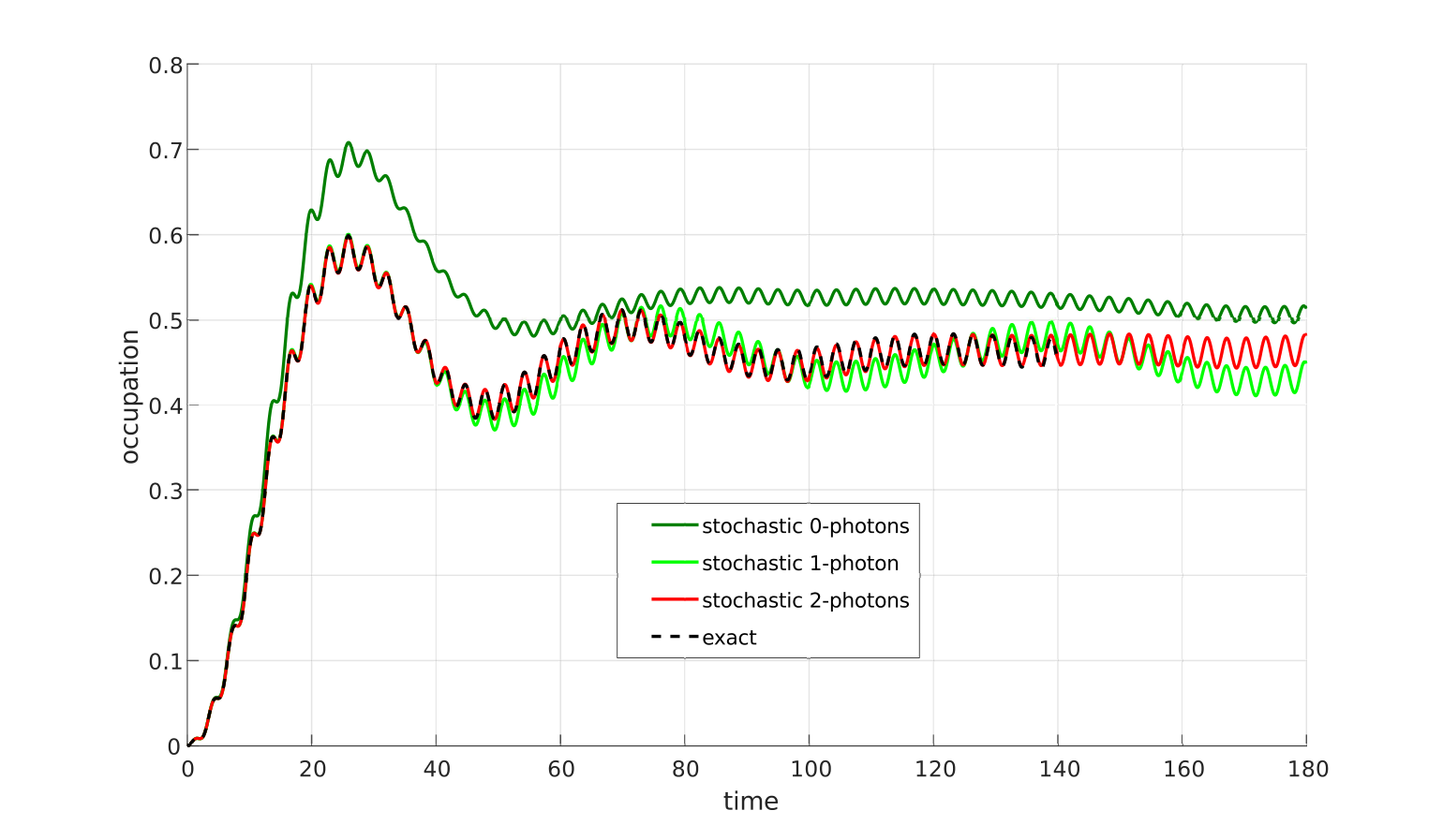
We consider the two cases, with the bath initially at zero temperature. The first case is when the impurity energy level is placed at the center of the bath’s energy band:
| (49) |
We calculated the occupation
| (50) |
of the equivalent qubit. In Fig. 5, we present the convergence of stochastic dressed wavefunction results with (only impurity Hilbert space, no virtual excitations), , and , to the exact results in the truncated Fock space.
The second case we considered is when the impurity energy level is placed at the edge of the bath energy band:
| (51) |
In Fig. 6 we show the convergence of results for the occupation of the equivalent qubit. In both cases the virtual excitations in were taken into account by including the first 20 sites of the bozonic chain.
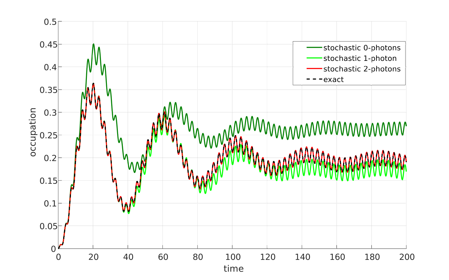
From the presented results we see that the convergence on the whole time interval is achieved with only two virtual excitations, whereas ED required to include the states with 8 excitations of the bath. This result confirms our idea that the stochastic dressed wavefunction method is capable of alleviating the exponential complexity of the real-time simulation.
Our approach is related to the conventional non-Markovian quantum state diffusion (NMQSD) methods [52, 53, 54, 55], but there is important difference between them. NMQSD includes only the impurity degrees of freedom, and the influence of the virtual cloud is represented through the functional derivative of the stochastic trajectory with respect to the noise. Since the functional derivative is a computationally complex object, a hierarchy of approximations is developed [55]. However, it is difficult to judge apriori how fast such a hierarchy would converge in the strong coupling regime. At the same time, the stochastic dressed wavefunction method takes into account the fact that the physical state of any open system is not restricted to the open system’s degrees of freedom, but surrounded by a cloud of virtual excitations. This way we obtain a clear physical picture of the major convergence factor: the dimension of the part of virtual cloud which is entangled to the impurity and which is statistically significant.
IV CONCULSION
In this work we present a novel numerically-exact simulation approach for the dynamics of quantum impurity models: the stochastic dressed wavefunction method. In this method, all the observable effects of the environment (irreversibly emitted excitations and the excitations due to finite occupation of the bath modes) are calculated by a Monte Carlo procedure without the sign problem. At the same time the unobservable virtual excitations are calculated by an exact diagonalization. We illustrate our method by providing the results of test calculations for the driven spin-boson model: only two virtual excitations are enough to achieve the uniform convergence on a large time interval.
Acknowledgements.
The study was founded by the RSF, grant 16-42-01057.References
- [1] A. C. Hewson, The Kodno Problem to Heavy Fermions (Cambridge University Press, Cambridge UK, 1997).
- [2] M. A. Kastner, Rev. Mod. Phys. 64, 849 (1992).
- [3] D. Goldhaber-Gordon, H. Shtrikman, D. Mahalu, D. Abusch-Magder, U. Meirav, and M. A. Kastner, Nature 391, 156 (1998).
- [4] H. C. Manoharan, C. P. Lutz, and D. M. Eigler, Nature 403, 512 (2000).
- [5] O. Agam and A. Schiller, Physical Review Letters 86, 484 (2001).
- [6] N. M. Zimmerman, B. Golding, and W. H. Haemmerle, Physical Review Letters 67, 1322 (1991).
- [7] B. Golding, N. M. Zimmerman, and S. N. Coppersmith, Physical Review Letters 68, 998 (1992).
- [8] J. Kondo, Physica B+C 125, 279 (1984).
- [9] H. Wipf, Physical Review Letters 52, 1308 (1984).
- [10] H. Grabert and H. R. Schober, “Theory of tunneling and diffusion of light interstitials in metals,” in Hydrogen in Metals III: Properties and Applications, edited by H. Wipf (Springer Berlin Heidelberg, Berlin, Heidelberg, 1997) pp. 5–49.
- [11] A. LeClair, F. Lesage, S. Lukyanov, and H. Saleur, Physics Letters A 235, 203 (1997).
- [12] K. Le Hur, Phys. Rev. B 85, 140506 (2012).
- [13] M. Goldstein, M. H. Devoret, M. Houzet, and L. I. Glazman, Phys. Rev. Lett. 110, 017002 (2013).
- [14] B. Peropadre, D. Zueco, D. Porras, and J. J. García-Ripoll, Phys. Rev. Lett. 111, 243602 (2013).
- [15] I. Snyman and S. Florens, Phys. Rev. B 92, 085131 (2015).
- [16] S. Bera, H. U. Baranger, and S. Florens, Phys. Rev. A 93, 033847 (2016).
- [17] D. Loss and D. P. DiVincenzo, Phys. Rev. A 57, 120 (1998).
- [18] R. Marcus and N. Sutin, Biochimica et Biophysica Acta (BBA) - Reviews on Bioenergetics 811, 265 (1985).
- [19] S. Tornow, R. Bulla, F. B. Anders, and A. Nitzan, Phys. Rev. B 78, 035434 (2008).
- [20] T. Pruschke, M. Jarrell, and J. Freericks, Advances in Physics 44, 187 (1995), https://doi.org/10.1080/00018739500101526 .
- [21] A. Georges, G. Kotliar, W. Krauth, and M. J. Rozenberg, Rev. Mod. Phys. 68, 13 (1996).
- [22] J. K. Freericks, V. M. Turkowski, and V. Zlatic, Phys. Rev. Lett. 97, 266408 (2006).
- [23] H. Aoki, N. Tsuji, M. Eckstein, M. Kollar, T. Oka, and P. Werner, Rev. Mod. Phys. 86, 779 (2014).
- [24] T. Maier, M. Jarrell, T. Pruschke, and M. H. Hettler, Rev. Mod. Phys. 77, 1027 (2005).
- [25] E. Gull, A. J. Millis, A. I. Lichtenstein, A. N. Rubtsov, M. Troyer, and P. Werner, Rev. Mod. Phys. 83, 349 (2011).
- [26] H. U. R. Strand, M. Eckstein, and P. Werner, Phys. Rev. X 5, 011038 (2015).
- [27] J. Panas, A. Kauch, J. Kuneš, D. Vollhardt, and K. Byczuk, Phys. Rev. B 92, 045102 (2015).
- [28] J. Panas, A. Kauch, and K. Byczuk, Phys. Rev. B 95, 115105 (2017).
- [29] H. Wong and Z.-D. Chen, Phys. Rev. B 77, 174305 (2008).
- [30] M. Vojta, Phys. Rev. B 85, 115113 (2012).
- [31] R. Egger, L. Mühlbacher, and C. H. Mak, Phys. Rev. E 61, 5961 (2000).
- [32] R. J. Needs, M. D. Towler, N. D. Drummond, and P. L. Ríos, Journal of Physics: Condensed Matter 22, 023201 (2010).
- [33] J. P. F. LeBlanc, A. E. Antipov, F. Becca, I. W. Bulik, G. K.-L. Chan, C.-M. Chung, Y. Deng, M. Ferrero, T. M. Henderson, C. A. Jiménez-Hoyos, E. Kozik, X.-W. Liu, A. J. Millis, N. V. Prokof’ev, M. Qin, G. E. Scuseria, H. Shi, B. V. Svistunov, L. F. Tocchio, I. S. Tupitsyn, S. R. White, S. Zhang, B.-X. Zheng, Z. Zhu, and E. Gull (Simons Collaboration on the Many-Electron Problem), Phys. Rev. X 5, 041041 (2015).
- [34] D. E. Makarov and N. Makri, Chemical Physics Letters 221, 482 (1994).
- [35] N. Makri, Journal of Mathematical Physics 36, 2430 (1995), https://doi.org/10.1063/1.531046 .
- [36] N. Makri and D. E. Makarov, The Journal of Chemical Physics 102, 4600 (1995), https://doi.org/10.1063/1.469508 .
- [37] N. Makri, E. Sim, D. E. Makarov, and M. Topaler, Proceedings of the National Academy of Sciences 93, 3926 (1996), http://www.pnas.org/content/93/9/3926.full.pdf .
- [38] H.-T. Chen, G. Cohen, and D. R. Reichman, The Journal of Chemical Physics 146, 054106 (2017a), https://doi.org/10.1063/1.4974329 .
- [39] D. Segal, A. J. Millis, and D. R. Reichman, Phys. Rev. B 82, 205323 (2010).
- [40] Y. Tanimura and R. Kubo, Journal of the Physical Society of Japan 58, 101 (1989), https://doi.org/10.1143/JPSJ.58.101 .
- [41] A. Ishizaki and G. R. Fleming, The Journal of Chemical Physics 130, 234111 (2009), https://doi.org/10.1063/1.3155372 .
- [42] J. Strümpfer and K. Schulten, Journal of Chemical Theory and Computation 8, 2808 (2012), pMID: 23105920, http://dx.doi.org/10.1021/ct3003833 .
- [43] M. Thoss, H. Wang, and W. H. Miller, The Journal of Chemical Physics 115, 2991 (2001), https://doi.org/10.1063/1.1385562 .
- [44] H. Wang, M. Thoss, and W. H. Miller, The Journal of Chemical Physics 115, 2979 (2001), https://doi.org/10.1063/1.1385561 .
- [45] H. Wang and M. Thoss, The Journal of Chemical Physics 119, 1289 (2003), https://doi.org/10.1063/1.1580111 .
- [46] H. Wang and M. Thoss, The Journal of Chemical Physics 138, 134704 (2013), https://doi.org/10.1063/1.4798404 .
- [47] G. Cohen, E. Gull, D. R. Reichman, and A. J. Millis, Phys. Rev. Lett. 115, 266802 (2015).
- [48] H.-T. Chen, G. Cohen, and D. R. Reichman, The Journal of Chemical Physics 146, 054105 (2017b), https://doi.org/10.1063/1.4974328 .
- [49] A. Kamenev, Field Theory of Non-Equilibrium Systems (Cambridge University Press, New York, 2011).
- [50] R. Feynman and F. Vernon, Annals of Physics 24, 118 (1963).
- [51] U. Weiss, Quantum dissipative systems, fourth edition (2012) pp. 1–566, cited By 58.
- [52] L. Diosi and W. T. Strunz, Phys. Lett. A 235, 569 (1997).
- [53] L. Diosi, N. Gisin, and W. T. Strunz, Phys.l Rev. A 58, 1699 (1998).
- [54] W. T. Strunz, Chemical Physics 268, 237 (2001).
- [55] R. Hartmann and W. T. Strunz, Journal of Chemical Theory and Computation , to appear.