Division of Particle and Astrophysical Science Nagoya University
Observational Constraint on Spherical Inhomogeneity
with CMB and Local Hubble Parameter
Abstract
We derive an observational constraint on a spherical inhomogeneity of the void centered at our position from the angular power spectrum of the cosmic microwave background(CMB) and local measurements of the Hubble parameter. The late time behaviour of the void is assumed to be well described by the so-called -Lemaître-Tolman-Bondi (LTB) solution. Then, we restrict the models to the asymptotically homogeneous models each of which is approximated by a flat Friedmann-Lemaître-Robertson-Walker model. The late time LTB models are parametrized by four parameters including the value of the cosmological constant and the local Hubble parameter. The other two parameters are used to parametrize the observed distance-redshift relation. Then, the LTB models are constructed so that they are compatible with the given distance-redshift relation. Including conventional parameters for the CMB analysis, we characterize our models by seven parameters in total. The local Hubble measurements are reflected in the prior distribution of the local Hubble parameter. As a result of a Markov-Chains-Monte-Carlo analysis for the CMB temperature and polarization anisotropies, we found that the inhomogeneous universe models with vanishing cosmological constant are ruled out as is expected. However, a significant under-density around us is still compatible with the angular power spectrum of CMB and the local Hubble parameter.
I Introduction
In observational cosmology, the global homogeneity and isotropy is a commonly unquestioned hypothesis, which is therefore called the cosmological principle. Actually, homogeneous and isotropic universe models have achieved great success to explain observational data and describe our universe. Nevertheless, it is interesting to ask how large magnitude of cosmological scale inhomogeneity can be compatible with the current cosmological observations. The observational test of the cosmological principle may be one of the most fundamental issues in cosmology just like old times. From this viewpoint, here we consider an observational constraint on cosmological scale inhomogeneity with the cosmic microwave background (CMB) and the local Hubble parameter. Since the isotropy of the universe is strongly supported by the isotropy of the CMB temperature, we focus on spherically symmetric inhomogeneous universe models.
Once we are allowed to be at the center of the universe with a spherical inhomogeneity, since most observables are limited on our past lightcone, the spatial inhomogeneity and temporal dependence may degenerate with each other. This fact gives one of the main difficulties in analyses of inhomogeneous universe models differently from homogeneous and isotropic universe models. Therefore, careful evaluation of observables and multi-directional analyses are important for the observational test of spherical inhomogeneity of our universe. We make a contribution to this issue from one direction in this paper.
Spherically symmetric dust universe models, so called the Lemaître-Tolman-Bondi (LTB) models [1, 2, 3], have been extensively studied in the last decade. The LTB models have been attracted much attention mainly as an alternative scenario to explain the apparent accelerated expansion of our universe without dark energy [4, 5, 6]. Actually, it is known that there exist the LTB models which can explain the observed luminosity distance redshift relation without a cosmological constant [5, 7, 8]. Especially, void-type inhomogeneity composed of growing modes has been actively studied because it can be compatible with the inflationary paradigm and the apparent accelerated expansion. Eventually, it has been revealed that the apparent accelerated expansion cannot be explained only by the radial inhomogeneity without a cosmological constant if we assume the standard cosmological history before the last scattering surface of CMB photons (see, e.g. Refs. [9, 10] for a detailed analysis).
In contrast, the models with a non-vanishing cosmological constant, namely, LTB models, have been studied not very often although we can find several restricted analyses [11, 10, 12, 13]. In this paper, we assume that the late time behaviour of our universe is well described by a LTB model. One remarkable feature in our approach is that we specify the spherically symmetric inhomogeneity by using the so-called inverse construction from a distance redshift relation. The same procedure is adopted in Ref. [14]. The inverse construction is a method to construct the LTB model in which the distance redshift relation for the central observer agrees with the designated one. In the case of LTB models, as is shown in Ref. [15], once the value of the cosmological constant is fixed and the angular diameter distance is specified as a function of the redshift, we can uniquely determine the LTB model. Therefore, the parameters to specify a LTB model are equivalent to the parameters contained in the distance redshift relation beside the value of the cosmological constant. In our analysis, the distance redshift relation is assumed to be given by the same form as the distance in the dust-dominated Friedmann-Lemaître-Robertson-Walker (FLRW) universe and parametrized by the Hubble constant and two fictitious cosmological parameters and . It should be emphasized that and are not necessarily related to the real matter density and the cosmological constant but just parameters to specify a distance redshift relation. This procedure is different from conventional methods of artificial direct parametrization of LTB models adopted in previous works (see, e.g. [16, 10]). Therefore, it could be possible to extract unknown effects of the spherical inhomogeneity around us.
In order to keep the predictability of the CMB anisotropy, we restrict our attention to asymptotically homogeneous models, and gradually connect each of the LTB models to a flat FLRW universe model. The connection is performed in the redshift interval , and the models are described by the standard homogeneous and isotropic universe models including relativistic energy components before . The late time LTB models are parametrized by four parameters including the value of the cosmological constant and the local Hubble parameter. Including conventional parameters for the CMB analysis, we characterize our models by seven parameters in total. For these seven parameters, we perform a Markov Chain Monte Carlo (MCMC) analysis by modifying the package CosmoMC11 1 http://cosmologist.info/cosmomc/readme.html. The local Hubble measurements are reflected in the prior distribution of the local Hubble parameter.
This paper is organized as follows. In Sec. II, we briefly review the inverse construction method reported in Ref. [15] and how to construct a universe model in the late time domain. The method to calculate the CMB angular power spectrum and the parameter set for the MCMC analysis is summarized in Sec. III. In Sec. IV, we show contour maps of the allowed regions for substantial parameters including the amplitude of the under-density. Sec. V is devoted to a summary and discussion.
In this paper, we use geometrized units in which the speed of light and Newton’s gravitational constant are one, respectively.
II Late time model construction
The LTB solution is the solution for the Einstein equations of the spherically symmetric dust fluid system. A line element of the LTB solution is written in the form:
| (1) |
where is the areal radius and is the function of the radial coordinate called the curvature function. From the Einstein equations with the cosmological constant , we obtain the following equation:
| (2) |
where is an arbitrary function of . The comoving energy density is given by
| (3) |
with . We can formally integrate Eq. (2) as
| (4) |
where is the function of which gives the bigbang time. The LTB solution has three arbitrary functions , and . Since the inhomogeneity associated with corresponds to decaying modes, we simply assume in this paper, where the constant value can be set to zero by shifting the origin of the time. In addition, by using the gauge degree of freedom to choose the radial coordinate , we set .
In Ref. [15], it is shown that, for , and the value of are uniquely determined, once the Hubble parameter and the normalized cosmological constant are fixed and the cosmological distance is given as a function of the redshift . In this paper, we use the same functional form of as that in the matter dominated homogeneous and isotropic universe models:
| (5) |
where and are the normalized matter density and the cosmological constant for the reference homogeneous and isotropic universe. It should be noted that and are not necessarily related to the real matter density and the cosmological constant but just parameters to specify the distance-redshift relation. For later convenience, we define as
| (6) |
where . Then, the LTB models are parametrized by the four parameters:, , and . Readers may refer to Ref. [15] for details of the construction method. Here we note that, by using above procedure, we can obtain the curvature function and the redshift as functions of the radial coordinate .
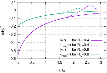
As is mentioned in Sec. I, we focus on the models each of which asymptotically coincides with a flat FLRW model. For this purpose, we gradually connect each LTB model to a flat FLRW universe model through the redshift domain , where we do not have significant observational constraints. Specifically, for , we assume the following form of the curvature function :
| (7) |
where is the redshift as a function of given for a LTB model specified by the four parameters:, , and , and
| (8) |
with (see Fig. 1 for the functional form of ).

Examples of the curvature function and are shown in Fig. 2.
In the higher redshift region, for accurate calculation of the CMB spectrum, we need to describe our universe taking the contribution of radiation components into account (Fig. 3). In this paper, we simply add the radiation components with the density at . Since the radiation effect for the dynamics of the universe is negligible for , the gap of the Hubble expansion rate at is negligible. Then the discontinuity of this procedure does not significantly affect the final results. Actually, we have confirmed that the results do not depend on the value of for .

III CMB anisotropy and the MCMC analysis
III.1 Angular power spectrum
For the calculation of the CMB temperature anisotropy, we use the open code CAMB 22 2 http://camb.info. Since homogeneous and isotropic universe models are supposed in this code, we need to appropriately modify input parameters and the output temperature anisotropy for our purpose. In this paper, we mainly focus on the primary effects on the CMB anisotropy, that is, we consider the temperature anisotropy that originates from inhomogeneity of the gravitational potential on the LSS. Inhomogeneity in our models are composed of growing modes, and it may significantly affect the secondary effects on the CMB anisotropy in low domain. Therefore, in our analysis, we simply ignore the angular power spectrum for .
In order to calculate observed at the center, we consider the fictitious flat FLRW universe which shares the same LSS with the inhomogeneous universe of our interest (see Fig. 3). We define the cosmological parameters, the angular diameter distance to LSS and the angular power spectrum in the fictitious FLRW model as , and , respectively. The cosmological parameters are fixed when we connect a late time LTB universe model to the corresponding flat FLRW universe model at . Then, the primary effects on the temperature anisotropy are given by those in the fictitious FLRW model, while the late time behaviour of the universe model is different from the homogeneous universe. Therefore we need to take the difference of the angular diameter distance between these models into account. Since we focus on , in this range, the flat-sky approximation is valid. In the flat-sky approximation, is given by the following form (see, e.g. [17])
| (9) |
where . The flat-sky approximation is valid in the accuracy of 1% for [18].
III.2 Parameter set for MCMC and calculation of
In order to describe the CMB anisotropy, in addition to the cosmological parameters for the late time universe model, we introduce the following three parameters: the scalar spectral index , amplitude of primordial fluctuation and baryon to matter ratio . In summary, we have the following seven free parameters:{, , , , , , }. In our analysis, we fix the optical depth as because the analysis does not use the low angular power spectrum, in which dependence is significant. We set a prior distribution for the Hubble parameter which is consistent with the observational value given in Ref. [19]. That is, we restrict the value of by using the Gaussian prior with , where the interval is the range.
Our procedure to calculate is summarized in Fig. 4. The calculation can be summarized in the following 4 steps.
- •
Step 1
- •
Step 2
Second, we fix the normalized baryon density and the dark matter density in the fictitious FLRW model as follows:
(10) (11) - •
Step 3
Then, we calculate which is the angular power spectrum observed at in the fictitious flat FLRW model by inputting the parameters: and to CAMB.
- •
Step 4
Finally, we perform the correction given in Eq. (9) to get .
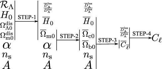
Because of the specification of CosmoMC, in the actual analysis, , , and are derived from another four parameters: , , and the ratio between the sound horizon and the angular diameter distance, where and is the dimensionless Hubble parameter defined as .
IV Results
First, we show posterior distributions and contour maps of , , , , and in Fig. 5, where is the void depth defined by
| (12) |
with being the initial time satisfying at the center.

The value of is closely correlated with the void depth . As is shown in this figure, is restricted at confidence level. This result explicitly shows the exclusion of void models. It should be noted that our prior models include the flat FLRW models with positive values of and also the inhomogeneous universe models with differently from the previous works not including . Therefore the comparison can be done within the common parameter space, and the exclusion is more explicit(see also Ref. [10]).
We show the posterior distribution of the void depth , and , with dependence by the color plot in Fig. 6.

Figure 6 shows that the smaller value of implies the larger value of the void depth . Once we fix the value of , tends to be smaller (deeper void) for the larger value of . This observation is consistent with the previous works [20, 13]. This dependence can be roughly understood as follows. If we increase the value of , the distance to the LSS decreases. On the other hand, we can increase the distance by making void depth deeper because the central region becomes closer to an open universe. Therefore, the correlation between and comes from the compensation of the distance to the LSS.
It is commonly expected that an under-dense region tends to increase the value of the local Hubble parameter compared to the asymptotic value given by CMB observations. However, in Fig. 5, the correlation between and is not clear. As is mentioned above, the reason for this behaviour comes from dependence of . Even if the value of is fixed at some value, changing the value of , we obtain a different profile of inhomogeneity and find a different value of . This dependence might help the resolution of the tension(see Ref. [21] for a recent analysis of the local , and Ref. [22] for possible explanations about the tension).
V Summary and discussion
We have discussed an observational constraint on the spherically symmetric inhomogeneous models by the CMB angular power spectrum and local Hubble parameter. We assumed that the late time cosmological models are well described by LTB models each of which is characterized by two parameters in the distance-redshift relation, the value of the cosmological constant and the local Hubble parameter . Connecting each of the late time inhomogeneous models to a flat homogeneous universe model, we calculated the CMB power spectrum observed at the center. The MCMC analysis with the Planck data [23] explicitly excluded inhomogeneous models with . However, at the same time, our results show that a significant amplitude of the under-density can be still compatible with the CMB angular power spectrum and the local Hubble measurement. We found that, even if we fix the amplitude of the void, the value of local Hubble parameter can change depending on the parameter , which specifies the inhomogeneity. This dependence could help to resolve the tension between the local measurement and CMB observations.
Finally, we list related important issues which we could not address in this paper. In Ref. [10], the strongest constraint for the amplitude of the inhomogeneity comes from the linear kinetic Snyaev-Zeldovich effect on the CMB power spectrum in large scales, and they concluded that the void amplitude is smaller than 0.29(see also Refs. [24, 25, 26, 27, 28, 29]). The Planck team reported the constraint on the kSZ monopole as for from the cluster SZ effect. This constraint may give much more stringent constraints on the void depth. The difference between the radial and transverse BAO scale may be also very efficient indicator for the spherical inhomogeneity(see, e.g., Refs. [30, 31, 32, 33]). In this paper, we ignored the angular power spectrum for lower multipoles. The spherical inhomogeneity may enhance the Integrated Sachs Wolfe(ISW) effect in the low multipoles. In order to clarify the significance of the spherical inhomogeneity to the ISW effect, we need to calculate the evolution of the perturbation with spherical inhomogeneity. The calculation of the perturbation is also needed for the calculation of the CMB lensing. We leave all these issues as future works.
Acknowledgements
This work was supported by JSPS KAKENHI Grant Numbers JP16K17688, JP16H01097 (CY) and JP16H01543 (KI).
References
- [1] G. Lemaitre, Gen. Rel. Grav. 29, 641 (1997), The expanding universe.
- [2] R. C. Tolman, Proc. Nat. Acad. Sci. 20, 169 (1934), Effect of imhomogeneity on cosmological models.
- [3] H. Bondi, Mon. Not. Roy. Astron. Soc. 107, 410 (1947), Spherically symmetrical models in general relativity.
- [4] I. Zehavi, A. G. Riess, R. P. Kirshner, and A. Dekel, Astrophys. J. 503, 483 (1998), arXiv:astro-ph/9802252, A Local Hubble Bubble from SNe Ia?
- [5] M.-N. Celerier, Astron. Astrophys. 353, 63 (2000), arXiv:astro-ph/9907206, Do we really see a cosmological constant in the supernovae data ?
- [6] K. Tomita, Astrophys. J. 529, 38 (2000), arXiv:astro-ph/9906027, Distances and lensing in cosmological void models.
- [7] H. Iguchi, T. Nakamura, and K.-i. Nakao, Prog. Theor. Phys. 108, 809 (2002), arXiv:astro-ph/0112419, Is dark energy the only solution to the apparent acceleration of the present universe?
- [8] C.-M. Yoo, T. Kai, and K.-i. Nakao, Prog. Theor. Phys. 120, 937 (2008), arXiv:0807.0932, Solving Inverse Problem with Inhomogeneous Universe.
- [9] M. Redlich, K. Bolejko, S. Meyer, G. F. Lewis, and M. Bartelmann, Astron. Astrophys. 570, A63 (2014), arXiv:1408.1872, Probing spatial homogeneity with LTB models: a detailed discussion.
- [10] W. Valkenburg, V. Marra, and C. Clarkson, Mon. Not. Roy. Astron. Soc. 438, L6 (2014), arXiv:1209.4078, Testing the Copernican principle by constraining spatial homogeneity.
- [11] V. Marra and M. Paakkonen, (2010), arXiv:1009.4193, Observational constraints on the LLTB model.
- [12] H. Negishi, K.-i. Nakao, C.-M. Yoo, and R. Nishikawa, Phys. Rev. D92, 103003 (2015), arXiv:1505.02472, Systematic error due to isotropic inhomogeneities.
- [13] K. Ichiki, C.-M. Yoo, and M. Oguri, Phys. Rev. D93, 023529 (2016), arXiv:1509.04342, Relationship between the CMB, Sunyaev-Zelfdovich cluster counts, and local Hubble parameter measurements in a simple void model.
- [14] P. Sundell, E. Mortsell, and I. Vilja, JCAP 1508, 037 (2015), arXiv:1503.08045, Can a void mimic the in CDM?
- [15] M. Tokutake and C.-M. Yoo, (2016), arXiv:1603.07837, Inverse Construction of the LTB Model from a Distance-redshift Relation.
- [16] J. Garcia-Bellido and T. Haugboelle, JCAP 0804, 003 (2008), arXiv:0802.1523, Confronting Lemaitre-Tolman-Bondi models with Observational Cosmology.
- [17] R. Durrer, The Cosmic Microwave Background (Cambridge University Press, 2008).
- [18] M. Vonlanthen, S. Rasanen, and R. Durrer, JCAP 1008, 023 (2010), arXiv:1003.0810, Model-independent cosmological constraints from the CMB.
- [19] G. Efstathiou, Mon. Not. Roy. Astron. Soc. 440, 1138 (2014), arXiv:1311.3461, H0 Revisited.
- [20] V. Marra, L. Amendola, I. Sawicki, and W. Valkenburg, Phys. Rev. Lett. 110, 241305 (2013), arXiv:1303.3121, Cosmic variance and the measurement of the local Hubble parameter.
- [21] A. G. Riess et al., Astrophys. J. 826, 56 (2016), arXiv:1604.01424, A 2.4% Determination of the Local Value of the Hubble Constant.
- [22] J. L. Bernal, L. Verde, and A. G. Riess, JCAP 1610, 019 (2016), arXiv:1607.05617, The trouble with .
- [23] Planck, P. A. R. Ade et al., (2015), arXiv:1502.01589, Planck 2015 results. XIII. Cosmological parameters.
- [24] J. Garcia-Bellido and T. Haugboelle, JCAP 0809, 016 (2008), arXiv:0807.1326, Looking the void in the eyes - the kSZ effect in LTB models.
- [25] C.-M. Yoo, K.-i. Nakao, and M. Sasaki, JCAP 1010, 011 (2010), arXiv:1008.0469, CMB observations in LTB universes: Part II – the kSZ effect in an LTB universe.
- [26] P. Zhang and A. Stebbins, (2010), arXiv:1009.3967, Confirmation of the Copernican principle at Gpc radial scale and above from the kinetic Sunyaev Zel’dovich effect power spectrum.
- [27] J. P. Zibin and A. Moss, Class. Quant. Grav. 28, 164005 (2011), arXiv:1105.0909, Linear kinetic Sunyaev-Zel’dovich effect and void models for acceleration.
- [28] P. Bull, T. Clifton, and P. G. Ferreira, Phys. Rev. D85, 024002 (2012), arXiv:1108.2222, The kSZ effect as a test of general radial inhomogeneity in LTB cosmology.
- [29] Planck, P. A. R. Ade et al., Astron. Astrophys. 561, A97 (2014), arXiv:1303.5090, Planck intermediate results. XIII. Constraints on peculiar velocities.
- [30] T. Biswas, A. Notari, and W. Valkenburg, (2010), arXiv:1007.3065, Testing the Void against Cosmological data: fitting CMB, BAO, SN and H0.
- [31] J. Garcia-Bellido and T. Haugboelle, JCAP 0909, 028 (2009), arXiv:0810.4939, The radial BAO scale and Cosmic Shear, a new observable for Inhomogeneous Cosmologies.
- [32] M. Zumalacarregui, J. Garcia-Bellido, and P. Ruiz-Lapuente, JCAP 1210, 009 (2012), arXiv:1201.2790, Tension in the Void: Cosmic Rulers Strain Inhomogeneous Cosmologies.
- [33] C. Clarkson, Comptes Rendus Physique 13, 682 (2012), arXiv:1204.5505, Establishing homogeneity of the universe in the shadow of dark energy.