跳到论文正文
W Papers独立论文阅读器 arXiv:1712.04201 论文正文 计算阅读时间 · 0%
引用这篇论文根据当前论文元数据生成,正式投稿前建议核对。


License: arXiv.org perpetual non-exclusive license
arXiv:1712.04201v1 [cs.NI] 12 Dec 2017

On the Energy-Efficient Deployment for Ultra-Dense Heterogeneous Networks with NLoS and LoS Transmissions

Bin Yang, Student Member, IEEE, Guoqiang Mao, \texorpdfstringFellow, IEEE, Xiaohu Ge, Senior Member, IEEE, Ming Ding, Senior Member, IEEE, Xuan Yang ††thanks: Correspondence author: Prof. Xiaohu Ge (Email: xhge@mail.hust.edu.cn, Tel: +86-27-87557941 ext 822).††thanks: Bin Yang, Xiaohu Ge and Xuan Yang are with the School of Electronic Information and Communications, Huazhong University of Science and Technology, China (Email: yangbin@hust.edu.cn, xhge@mail.hust.edu.cn, xuan_yan9@163.com). ††thanks: Guoqiang Mao is with the School of Computing and Communication, The University of Technology Sydney, Australia (e-mail: g.mao@ieee.org). ††thanks: Ming Ding is with Data61, CSIRO, Australia (Email: ming.ding@data61.csiro.au).
Abstract

We investigate network performance of ultra-dense heterogeneous networks (HetNets) and study the maximum energy-efficient base station (BS) deployment incorporating probabilistic non-line-of-sight (NLoS) and line-of-sight (LoS) transmissions. First, we develop an analytical framework with the maximum instantaneous received power (MIRP) and the maximum average received power (MARP) association schemes to model the coverage probability and related performance metrics, e.g., the potential throughput (PT) and the energy efficiency (EE). Second, we formulate two optimization problems to achieve the maximum energy-efficient deployment solution with \texorpdfstringspecific service criteria. Simulation results show that there are tradeoffs among the coverage probability, the total power consumption\texorpdfstring, and the EE. To be specific, the maximum coverage probability with ideal power consumption is superior to that with practical power consumption when the total power constrain\texorpdfstringt is small and inferior to that with practical power consumption when the total power constrain\texorpdfstringt becomes large. Moreover, the maximum EE is a decreasing function with respect to the coverage probability constrain\texorpdfstringt.

Index Terms:
Ultra-Dense HetNets, non-line-of-sight (NLoS), line-of-sight (LoS), Poisson point process (PPP), energy efficiency (EE), optimization, cell association scheme.

I Introduction

Ultra-dense deployment of small cell base stations (BSs), relay nodes, and distributed antennas is considered as a de facto solution for realizing the significant performance improvements needed to accommodate the overwhelming future mobile traffic demand\texorpdfstring [1]. Traditional network expansion techniques like cell splitting are often utilized by telecom operators to achieve the expected throughput, which \texorpdfstringis less efficient and proven not to keep up with the pace of traffic proliferation in the near future. Heterogeneous networks (HetNets) then become a promising and attractive network architecture to alleviate the problem. “HetNets” is a broad term that refers to the coexistence of different networks (e.g., traditional macrocells and small cell networks like femtocells and picocells), each of them constituting a network tier. Due to differences in deployment, BSs in different tiers may have different transmit powers, radio access technologies, fading environments and spatial densities. HetNets are envisioned to change the existing network architectures and have been introduced in the LTE-Advanced standardization [2, 3].

Massive work has been done in HetNets scenario mainly related \texorpdfstringto cell association scheme [4, 5, 6], cache-enabled networks [7], physical layer security [8], etc. In [4], the pertinent user association algorithms designed for HetNets, massive MIMO networks, mmWave scenarios and energy harvesting networks have been surveyed for the future fifth generation (5G) networks. Bethanabhotla et al. [5] investigated the optimal user-cell association problem for massive MIMO HetNets and illustrated how massive MIMO \texorpdfstringcould also provide nontrivial advantages at the system level. The joint downlink cell association and wireless backhaul bandwidth allocation in a two-tier HetNet is studied in [6]. In [7], Yang et al. aimed to model and evaluate the performance of the wireless HetNet where the radio access network (RAN) caching and device-to-device (D2D) caching coexist. The physical layer security of HetNets where the locations of all BSs, \texorpdfstringmobile users (MUs\texorpdfstring) and eavesdroppers are modeled as independent homogeneous PPPs in [8].

From the mobile operators point of view, the commercial viability of network \texorpdfstringdensification depends on the underlying capital and operational expenditure [9]. While the former cost may be covered by taking up a high volume of customers, with the rapid rise in the price of energy, and given that BSs are particularly power-hungry, energy efficiency (EE) has become an increasingly crucial factor for the success of dense HetNets [10]. Recently, loads of work [11, 12, 13, 14, 15] has investigated the EE in the 5G network scenarios. In [11], Niu et al. investigated the problem of minimizing the energy consumption via optimizing concurrent transmission scheduling and power control for the mmWave backhauling of small cells densely deployed in HetNets. A self-organized cross-layer optimization for enhancing the EE of the D2D communications without creating harmful impact on other tiers by employing a non-cooperative game in a three-tier HetNet is proposed in [12]. To jointly optimize the EE and video quality, Wu et al. [13] presented an energy-quality aware bandwidth aggregation scheme. In [14], Yang et al. investigated the energy-efficient resource allocation problem for downlink heterogeneous OFDMA networks. The mobile edge computing offloading mechanisms are studied in 5G HetNets [15].

Different from most prior work analyzing network performance where the propagation path loss between the BSs and the MUs\texorpdfstring follows the same power-law model, in this paper we consider the co-existence of both non-line-of-sight (NLoS) and line-of-sight (LoS) transmissions, which frequently occur in urban areas. More specifically, for a randomly selected MU, BSs deployed according to a homogeneous Poisson point process (PPP) are divided into two categories, i.e., NLoS BSs and LoS BSs, depending on the distance between BSs and MUs. \texorpdfstringIt is well known that LoS transmission may occur when the distance between a transmitter and a receiver is small, and NLoS transmission is common in office environments and central business districts. Moreover, as the trend of ultra-dense network deployment, the distance between a transmitter and a receiver decreases, the probability that a LoS path exists between them increases, thereby causing a transition from NLoS transmission to LoS transmission with a higher probability [16]. In this context, Ding et al. [16] studied the coverage and capacity performance by using a multi-slop path loss model incorporating probabilistic NLoS and LoS transmissions. The coverage and capacity performance in millimeter wave cellular networks are studied in [17, 18, 19]. In [17], a three-state statistical model for each link was assumed, in which a link can either be in a\texorpdfstringn NLoS, LoS or an outage state. In [18], self-backhauled millimeter wave cellular networks are characterized assuming a cell association scheme based on the smallest path loss. However, both [17] and [18] assume a noise-limited network, ignoring inter-cell interference, which may not be very practical since modern wireless networks work in the interference-limited region. \texorpdfstringIn [19], the coverage probability and capacity were calculated in a millimeter wave cellular network based on the smallest path loss cell association model assuming multi-path fading modeled as Nakagami-mm fading, respectively. However, shadowing was ignored in their models, which may not be very practical for an ultra-dense heterogeneous network.

In contrast to prior work, we investigate the HetNets in a more realistic scenario, i.e., NLoS and LoS transmissions\texorpdfstring in desired signal and interference signal are both considered. Besides, we also explore the optimal BS deployment under the quality of service (QoS) constrain\texorpdfstringt. The main contributions of this paper are summarized as follows:

  1. 1.
    \texorpdfstring

    A unified framework: We propose a unified framework, in which the user association strategies based on the maximum instantaneous received power (MIRP) and the maximum average received power (MARP) can be studied, assuming log-normal shadowing, Rayleigh fading and incorporating probabilistic NLoS and LoS transmissions.

  2. 2.

    Performance optimization: We formulate two optimization problems under different QoS constrain\texorpdfstringts, i.e., the maximal total power consumption and the minimal coverage probability. Utilizing solutions of the above optimization problems, the maximum energy-efficient BS deployment is obtained.

  3. 3.

    Network design insights: We compare the optimal BS deployment strategies in different network scenarios, i.e., assuming the fixed transmit power, the density-dependent transmit power, with and without considering the static power consumption in BSs. Through our results, the maximum coverage probability with ideal power consumption is superior to that with practical power consumption when the total power constrain\texorpdfstringt is small and inferior to that with practical power consumption when the total power constrain\texorpdfstringt becomes large. Moreover, the maximum EE is a decreasing function with respect to the coverage probability constrain\texorpdfstringt.

The \texorpdfstringremainder of this paper is organized as follows. Section II introduces the system model, network assumptions\texorpdfstring, and performance metrics. In section III, the coverage probability, the potential throughput (PT) and the EE of the HetNets are derived with the MIRP and the MARP association schemes, respectively. In Section IV, two optimization problems for energy-efficient BS deployment are formulated. In Section V, the analytical results are validated via Monte Carlo simulations. Besides, the insights of BS deployment are studied. Finally, Section VI concludes this paper and discusses possible future work.

II System Model

In this paper, a KK-tier HetNet is considered, which consists of macrocells, picocells, femtocells, etc. BSs of each tier are assumed to be spatially distributed on the infinite plane and locations of BSs follow independent homogeneous Poisson point processes (HPPPs) denoted by Φk={𝑿k,i}\Phi_{k}=\left\{\boldsymbol{X}_{k,i}\right\} with \texorpdfstringa density (aka intensity) λk\lambda_{k}, k∈{1,2,⋯,K}​=def​𝒦k\in\left\{1,2,\cdots,K\right\}\overset{\textrm{def}}{=}\mathcal{K} 11 1 x​=def​yx\overset{\textrm{def}}{=}y means xx is defined to be another name for yy., where 𝑿k,i\boldsymbol{X}_{k,i} denotes the location of BS in the kk-th tier. MUs are deployed according to another independent HPPP denoted by Φu\Phi_{u} with \texorpdfstringa density λu\lambda_{u} (λu≫λk\lambda_{u}\gg\lambda_{k}). BSs belonging to the same tier transmit using the same constant power PkP_{k} and sharing the same bandwidth. Besides, within a cell assume that each MU uses orthogonal multiple access method to connect to a serving BS for downlink and uplink transmissions and therefore there is no intra-cell interference in the analysis of our paper. However, adjacent BSs which are not serving the connected MU may cause inter-cell interference which is the main focus of this paper. It is further assumed that each MU can possibly associate with a BS belonging to any tier, i.e., open access policy is employed.

\texorpdfstring

Without loss of generality and from the Slivnyak’s Theorem [20], we consider the typical MUwhich is usually assumed to be located at the origin, as the focus of our performance analysis.

II-A Signal Propagation Model

The long-distance signal attenuation in tier kk is modeled by a monotone, non-increasing and continuous path loss function lk:[0,∞]↦[0,∞]l_{k}:\left[0,\infty\right]\mapsto\left[0,\infty\right] and lkl_{k} decays to zero asymptotically. The fast fading coefficient for the wireless link between a BS 𝑿k,i∈Φk\boldsymbol{X}_{k,i}\in\Phi_{k} and the typical MU is denoted as h𝑿k,ih_{\boldsymbol{X}_{k,i}}. {h𝑿k,i}\left\{h_{\boldsymbol{X}_{k,i}}\right\} are assumed to be random variables which are mutually independent and identically distributed (i.i.d.) and also independent of BS locations {𝑿𝒌,𝒊}\left\{\boldsymbol{\boldsymbol{X}_{k,i}}\right\}, thus h𝑿k,ih_{\boldsymbol{X}_{k,i}} can be denoted as hkh_{k} for the sake of simplicity. Similarly, the shadowing is denoted by gkg_{k} and particularly assume that it follows a log-normal distribution with zero mean and standard deviation σ\sigma. Note that the proposed model is general enough to account for various propagation scenarios with fasting fading, shadowing, and different path loss models.

To characterize shadowing effect in urban areas which is a unique scenario in our analysis, both NLoS and LoS transmissions are incorporated. That is, if the visual path between a BS 𝑿k,i∈Φk\boldsymbol{X}_{k,i}\in\Phi_{k} and the typical MU is blocked by obstacles like buildings, trees\texorpdfstring, and even MUs, it is a\texorpdfstringn NLoS transmission\texorpdfstring. \texorpdfstringOtherwise it is a LoS transmission. The occurrence of NLoS and LoS transmissions depend on various environmental factors, including geographical structure, distance\texorpdfstring, and cluster. In this work, a one-parameter distance-based NLoS/LoS transmission probability model is applied. That is,

pkNL​(‖𝑿k,i‖)+pkL​(‖𝑿k,i‖)=1,p_{k}^{\textrm{NL}}\left(\left\|\boldsymbol{X}_{k,i}\right\|\right)+p_{k}^{\textrm{L}}\left(\left\|\boldsymbol{X}_{k,i}\right\|\right)=1, (1)

where pkNL​(‖𝑿k,i‖)p_{k}^{\textrm{NL}}\left(\left\|\boldsymbol{X}_{k,i}\right\|\right) and pkL​(‖𝑿k,i‖)p_{k}^{\textrm{L}}\left(\left\|\boldsymbol{X}_{k,i}\right\|\right) denote the probability of the occurrence of NLoS and LoS transmissions, respectively, ‖𝑿k,i‖\left\|\boldsymbol{X}_{k,i}\right\| is the distance between the BS 𝑿k,i\boldsymbol{X}_{k,i} and the typical MU.

Regarding the mathematical form of pkL​(‖𝑿k,i‖)p_{k}^{\textrm{L}}\left(\left\|\boldsymbol{X}_{k,i}\right\|\right) (or pkNL​(‖𝑿k,i‖)p_{k}^{\textrm{NL}}\left(\left\|\boldsymbol{X}_{k,i}\right\|\right)), Blaunstein et al. [21] formulated pkL​(‖𝑿k,i‖)p_{k}^{\textrm{L}}\left(\left\|\boldsymbol{X}_{k,i}\right\|\right) as a negative exponential function, i.e., pkL​(‖𝑿k,i‖)=e−κ​‖𝑿k,i‖p_{k}^{\textrm{L}}\left(\left\|\boldsymbol{X}_{k,i}\right\|\right)=e^{-\kappa\left\|\boldsymbol{X}_{k,i}\right\|}, where κ\kappa is a parameter determined by the density and the mean length of the blockages lying in the visual path between BSs and the typical MU. Bai et al. [22] extended Blaunstein’s work by using random shape theory which shows that κ\kappa is not only determined by the mean length but also the mean width of the blockages. [17] and [19] approximated pkL​(‖𝑿k,i‖)p_{k}^{\textrm{L}}\left(\left\|\boldsymbol{X}_{k,i}\right\|\right) by using piece-wise functions and step functions, respectively. Ding et al. [16] considered pkL​(‖𝑿k,i‖)p_{k}^{\textrm{L}}\left(\left\|\boldsymbol{X}_{k,i}\right\|\right) to be a linear function and a two-piece exponential function, respectively; both are recommended by the 3GPP. It is important to note that the introduction of NLoS and LoS transmissions is essential to model practical networks, where a MU does not necessarily have to connect to the nearest BS. Instead, for many cases, MUs are associated with farther BSs with stronger signal strength.

It should be noted that the occurrence of NLoS and LoS transmissions is assumed to be independent for different BS-MU pairs. Though such assumption might not be entirely realistic (e.g., NLoS transmission caused by a large obstacle may be spatially correlated), Bai et al. [22, 19] showed that the impact of the independence assumption on the SINR analysis is negligible.

For a specific tier kk, note that from the viewpoint of the typical MU, each BS in the infinite plane ℝ2\mathbb{R}^{2} is either a\texorpdfstringn NLoS BS or a LoS BS to the typical MU. Accordingly, a thinning procedure on points in the PPP Φk\Phi_{k} is performed to model the distributions of NLoS BSs and LoS BSs, respectively. That is, each BS in Φk\Phi_{k} will be kept if a BS has a\texorpdfstringn NLoS transmission with the typical MU, thus forming a new point process denoted by ΦkNL\Phi_{k}^{\textrm{NL}} . While BSs in Φk∖ΦkNL\Phi_{k}\setminus\Phi_{k}^{\textrm{NL}} form another point process denoted by ΦkL\Phi_{k}^{\textrm{L}}, representing the set of BSs with LoS path to the typical MU. As a consequence of the independence assumption of NLoS and LoS transmissions mentioned in the last paragraph, ΦkNL\Phi_{k}^{\textrm{NL}} and ΦkL\Phi_{k}^{\textrm{L}} are two independent non-homogeneous PPPs with intensity functions λk​pkNL​(‖𝑿k,i‖)\lambda_{k}p_{k}^{\textrm{NL}}\left(\left\|\boldsymbol{X}_{k,i}\right\|\right) and λk​pkL​(‖𝑿k,i‖)\lambda_{k}p_{k}^{\textrm{L}}\left(\left\|\boldsymbol{X}_{k,i}\right\|\right), respectively.

Based on assumptions above, the received power of the typical MU from a BS 𝑿k,i∈Φk\boldsymbol{X}_{k,i}\in\Phi_{k} is defined as follows.

\texorpdfstring

Definitation 1. The received power of the typical MU from a BS 𝑿k,i∈Φk\boldsymbol{X}_{k,i}\in\Phi_{k} , i.e., Pk,irecP_{k,i}^{\textrm{rec}} is

Pk,irec={Pk,iNL=Pk​AkNL​hkNL​gkNL​lkNL​(‖𝑿k,i‖),with probability ​pkNL​(‖𝑿k,i‖)Pk,iL=Pk​AkL​hkL​gkL​lkL​(‖𝑿k,i‖),with probability ​pkL​(‖𝑿k,i‖),P_{k,i}^{\textrm{rec}}=\begin{cases}P_{k,i}^{\textrm{NL}}=P_{k}A_{k}^{\textrm{NL}}h_{k}^{\textrm{NL}}g_{k}^{\textrm{NL}}l_{k}^{\textrm{NL}}\left(\left\|\boldsymbol{X}_{k,i}\right\|\right),&\hskip-8.5359pt\textrm{with probability }p_{k}^{\textrm{NL}}\left(\left\|\boldsymbol{X}_{k,i}\right\|\right)\\ P_{k,i}^{\textrm{L}}=P_{k}A_{k}^{\textrm{L}}h_{k}^{\textrm{L}}g_{k}^{\textrm{L}}l_{k}^{\textrm{L}}\left(\left\|\boldsymbol{X}_{k,i}\right\|\right),&\hskip-8.5359pt\textrm{with probability }p_{k}^{\textrm{L}}\left(\left\|\boldsymbol{X}_{k,i}\right\|\right)\end{cases}, (2)
\texorpdfstring

where AkNLA_{k}^{\textrm{NL}} and AkLA_{k}^{\textrm{L}} denote the respective path loss for NLoS and LoS transmissions at the reference distance (usually at 1 meter). For simplicity, denote BkU=Pk​AkUB_{k}^{\textrm{U}}=P_{k}A_{k}^{\textrm{U}} and let lkU​(‖𝑿k,i‖)=‖𝑿k,i‖−αkUl_{k}^{\textrm{U}}\left(\left\|\boldsymbol{X}_{k,i}\right\|\right)=\left\|\boldsymbol{X}_{k,i}\right\|^{-\alpha_{k}^{\textrm{U}}}, where the superscript U∈{NL,L}​=def​𝒰\textrm{U}\in\left\{\textrm{NL},\textrm{L}\right\}\overset{\textrm{def}}{=}\mathcal{U} used distinguishes NLoS and LoS transmissions and αkU\alpha_{k}^{\textrm{U}} denotes the path loss exponent for NLoS or LoS transmission in the kk-th tier. Recently, [23] and [24] took bounded path loss model and stretched exponential path loss model into consideration, in which several interesting performance trends are found and will be investigated in our future work.

\texorpdfstring

Remark 1. Apart from the fixed transmit power, a density-dependent transmit power is further assumed and analyzed mentioned in [25], i.e., Pk​(λ)=10Tk10​ηAkNL​rk−αkNLP_{k}\left(\lambda\right)=\frac{10^{\frac{T_{k}}{10}\eta}}{A_{k}^{\textrm{NL}}r_{k}^{-\alpha_{k}^{\textrm{NL}}}}, where rk=1π​λkr_{k}=\sqrt{\frac{1}{\pi\lambda_{k}}} is the radius of an equivalent disk-shaped coverage area in the kk-th tier with an area size of rk=1πr_{k}=\sqrt{\frac{1}{\pi}}\texorpdfstring and TkT_{k} is the per tier SINR threshold.

II-B Cell Association Scheme

Cell association scheme\texorpdfstring [26] plays a \texorpdfstringcrucial role in network performance determining BS coverage, MU hand-off regulation and even facility deployment of small cells. Conventionally, a typical MU is connected to the BS 𝑿k,m\boldsymbol{X}_{k,m} if and only if

𝒫k,mdBm>𝒫j,ndBm,j≠k,\mathcal{\mathcal{P}}_{k,m}^{\textrm{dBm}}>\mathcal{\mathcal{P}}_{j,n}^{\textrm{dBm}},j\neq k, (3)

where 𝒫k,mdBm\mathcal{\mathcal{P}}_{k,m}^{\textrm{dBm}} is the instantaneous received power with dBm unit from the BS 𝑿k,m\boldsymbol{X}_{k,m} and Eq. (3) is known as the MIRP association scheme.

In practical, 𝒫kdBm\mathcal{\mathcal{P}}_{k}^{\textrm{dBm}} is usually averaged out in time and frequency domains to cope with fluctuations caused by channel fading. In this text, a typical MU is connected to the BS 𝑿k,m\boldsymbol{X}_{k,m} if and only if

𝒫k,mdBm¯>𝒫j,ndBm¯,j≠k,\overline{\mathcal{\mathcal{P}}_{k,m}^{\textrm{dBm}}}>\overline{\mathcal{\mathcal{P}}_{j,n}^{\textrm{dBm}}},j\neq k, (4)

where 𝒫k,mdBm¯\overline{\mathcal{\mathcal{P}}_{k,m}^{\textrm{dBm}}} denotes the average received power with dBm unit from the BS 𝑿k,m\boldsymbol{X}_{k,m} and Eq. (4) is known as the MARP association scheme.

Aided by cell range expansion (CRE), which is realized by MUs adding a positive cell range expansion bias (CREB) to the received power from BSs in different tiers, more MUs can be offloaded to small cells. That is, if a MU is associated with the BS 𝑿k,m\boldsymbol{X}_{k,m} if and only if

𝒫k,mdBm¯+△k,mdB>𝒫j,ndBm¯+△j.ndB,j≠k,\overline{\mathcal{\mathcal{P}}_{k,m}^{\textrm{dBm}}}+\triangle_{k,m}^{\textrm{dB}}>\overline{\mathcal{\mathcal{P}}_{j,n}^{\textrm{dBm}}}+\triangle_{j.n}^{\textrm{dB}},j\neq k, (5)

where △k,mdB\triangle_{k,m}^{\textrm{dB}} and △j,ndB\triangle_{j,n}^{\textrm{dB}}is the CREB with dB unit in the kk-th and jj-th tier. With proper CREB chosen, the coverage of BSs in some tiers is artificially expanded, allowing MUs more \texorpdfstringflexible to be associated with BSs which may not provide the strongest received power, thus balancing traffic load to achieve spatial efficiency. However, CRE causes severe interference to small cell MU which impair the QoS of small cell users and thus almost blank subframes (ABS) coordination is needed between macrocell BSs and small cell BSs. However, the analysis of CRE plus ABS is challenging because (i) the association scheme is not only determined by the received power but also the current resource allocation strategy, and (ii) ignoring ABS while using CRE can impair the coverage performance. For simplicity, CRE and ABS are not going to be considered in this paper, which are left as our future work.

II-C Performance Metrics

To evaluate the network performance, the following three metrics, i.e., the coverage probability, the PT and the EE, are focused on.

The coverage probability is the probability that the received SINR is greater than a given threshold, i,e, pcov({λk},{Tk},{BkU})=Pr[∪k∈𝒦,𝑿k,i∈ΦkSINRk(‖𝑿k,i‖)>Tk]p_{\textrm{cov}}\left(\left\{\lambda_{k}\right\},\left\{T_{k}\right\},\left\{B_{k}^{\textrm{U}}\right\}\right)=\Pr\Bigl[\underset{k\in\mathcal{K},\boldsymbol{X}_{k,i}\in\Phi_{k}}{\cup}\textrm{SINR}_{k}\left(\left\|\boldsymbol{X}_{k,i}\right\|\right)>T_{k}\Bigr], where SINRk​(‖𝑿k,i‖)\textrm{SINR}_{k}\left(\left\|\boldsymbol{X}_{k,i}\right\|\right) is defined as follows

SINRk​(‖𝑿k,i‖)=Pk​AkU​hkU​gkU​lkU​(‖𝑿k,i‖)∑∑𝑿k,j∈Φk∖𝑿k,i​Pk​AkU​hkU​gkU​lkU​(‖𝑿k,j‖)+η,\textrm{SINR}_{k}\left(\left\|\boldsymbol{X}_{k,i}\right\|\right)=\frac{P_{k}A_{k}^{\textrm{U}}h_{k}^{\textrm{U}}g_{k}^{\textrm{U}}l_{k}^{\textrm{U}}\left(\left\|\boldsymbol{X}_{k,i}\right\|\right)}{\mathrel{{\mathop{\sum}\limits}}\underset{\boldsymbol{X}_{k,j}\in\Phi_{k}\setminus\boldsymbol{X}_{k,i}}{\sum}P_{k}A_{k}^{\textrm{U}}h_{k}^{\textrm{U}}g_{k}^{\textrm{U}}l_{k}^{\textrm{U}}\left(\left\|\boldsymbol{X}_{k,j}\right\|\right)+\eta}, (6)

where Φk∖𝑿k,i\Phi_{k}\setminus\boldsymbol{X}_{k,i} is the Palm point process [27] representing the set of interfering BSs in the kk-th tier and η\eta denotes the noise power at the MU side, which is assumed to be the additive white Gaussian noise (AWGN).

The PT is defined as follows [28, 24]

𝒯⁡({λk},{Tk},{BkU})=∑λk​𝒜k​pcov,kcond​log2⁡(1+Tk)=∑λk​pcov,k​log2⁡(1+Tk),\mathcal{T}\left(\left\{\lambda_{k}\right\},\left\{T_{k}\right\},\left\{B_{k}^{\textrm{U}}\right\}\right)=\mathrel{{\mathop{\sum}\limits}}\lambda_{k}\mathcal{A}_{k}p_{\textrm{cov},k}^{\textrm{cond}}\log_{2}\left(1+T_{k}\right)=\mathrel{{\mathop{\sum}\limits}}\lambda_{k}p_{\textrm{cov},k}\log_{2}\left(1+T_{k}\right), (7)

where the network is fully loaded due to the assumption that λu≫λk\lambda_{u}\gg\lambda_{k}, 𝒜k\mathcal{A}_{k} is the association probability that the typical MU is connected to the kk-th tier, pcov,kcondp_{\textrm{cov},k}^{\textrm{cond}} is the conditional association coverage probability and pcov,kp_{\textrm{cov},k} is the per-tier coverage probability. Compared with the area spectral efficiency (ASE), which is defined as

ASE​({λk},{Tk},{BkU})=∑𝔼⁡[λk​log2⁡(1+SINRk​(‖𝑿k,i‖))],\textrm{ASE}\left(\left\{\lambda_{k}\right\},\left\{T_{k}\right\},\left\{B_{k}^{\textrm{U}}\right\}\right)=\mathrel{{\mathop{\sum}\limits}}\mathbb{E}\left[\lambda_{k}\log_{2}\left(1+\textrm{SINR}_{k}\left(\left\|\boldsymbol{X}_{k,i}\right\|\right)\right)\right], (8)

the PT implicitly assumes a fixed rate transmission from all BSs in the network, and has a unit of bps/Hz/m2\textrm{bps/Hz/m}^{2}, while the ASE assumes full buffers but it allows each link to adapt its rate to the optimal value for a given SINR, thus avoiding outages at low SINR and the wasting of rate at high SINR [24]. In other words, the PT is a more realistic performance metric and the ASE upper bounds the PT. In our analysis, the PT is chosen as our performance metric.

The EE is defined as the ratio between the PT and the total energy consumption of the network, i.e.,

ℰ⁡({λk},{Tk},{BkU})=𝒯⁡({λk},{Tk},{BkU})∑λk​(ak​Pk+bk),\mathcal{E}\left(\left\{\lambda_{k}\right\},\left\{T_{k}\right\},\left\{B_{k}^{\textrm{U}}\right\}\right)=\frac{\mathcal{T}\left(\left\{\lambda_{k}\right\},\left\{T_{k}\right\},\left\{B_{k}^{\textrm{U}}\right\}\right)}{\mathrel{{\mathop{\sum}\limits}}\lambda_{k}\left(a_{k}P_{k}+b_{k}\right)}, (9)

where the coefficient aka_{k} accounts for power consumption that scales with the average radiated power, and the term bkb_{k} models the static power consumed by signal processing, battery backup and cooling [29]. Other performance metrics, such as the bit-error probability and per-MU data rate, can be found using the coverage probability (SINR distribution) following the methods mentioned in [30].

III Performance Analysis

In this section, we derive expressions for the considered performance metrics and study the effect of densification on these metrics. It is started by introducing the network transformation and then presenting the analytical expressions with the MIRP and MARP association schemes in the following subsections.

III-A Network Transformation

Before presenting our main analytical results, firstly the network transformation is introduced, which aims to unify the analysis and to reduce the complexity as well.

Using the manipulation in [31, 32], we define

Rk,iNL¯=‖𝑿k,i‖⋅(BkNLgkNL)−1/αkNL,\overline{R_{k,i}^{\textrm{NL}}}=\left\|\boldsymbol{X}_{k,i}\right\|\cdot\left(B_{k}^{\textrm{NL}}g_{k}^{\textrm{NL}}\right)^{-1/\alpha_{k}^{\textrm{NL}}}, (10)

and

Rk,iL¯=‖𝑿k,i‖⋅(BkLgkL)−1/αkL,\overline{R_{k,i}^{\textrm{L}}}=\left\|\boldsymbol{X}_{k,i}\right\|\cdot\left(B_{k}^{\textrm{L}}g_{k}^{\textrm{L}}\right)^{-1/\alpha_{k}^{\textrm{L}}}, (11)

respectively. Then Eq. (2) can be written as

Pk,irec={Pk,iNL=hkNL​(Rk,iNL¯)−αkNL,with probability ​pkNL​(‖𝑿k,i‖)Pk,iL=hkL​(Rk,iL¯)−αkL,with probability ​pkL​(‖𝑿k,i‖).P_{k,i}^{\textrm{rec}}=\begin{cases}P_{k,i}^{\textrm{NL}}=h_{k}^{\textrm{NL}}\left(\overline{R_{k,i}^{\textrm{NL}}}\right)^{-\alpha_{k}^{\textrm{NL}}},&\hskip-8.5359pt\textrm{with probability }p_{k}^{\textrm{NL}}\left(\left\|\boldsymbol{X}_{k,i}\right\|\right)\\ P_{k,i}^{\textrm{L}}=h_{k}^{\textrm{L}}\left(\overline{R_{k,i}^{\textrm{L}}}\right)^{-\alpha_{k}^{\textrm{L}}},&\hskip-8.5359pt\textrm{with probability }p_{k}^{\textrm{L}}\left(\left\|\boldsymbol{X}_{k,i}\right\|\right)\end{cases}. (12)

By adopting the Equivalence Theorem in [31], it is concluded that the distance {Rk,iNL¯}i\left\{\overline{R_{k,i}^{\textrm{NL}}}\right\}_{i} (or {Rk,iL¯}i\left\{\overline{R_{k,i}^{\textrm{L}}}\right\}_{i}) \texorpdfstringfrom a scaled point process for NLoS BSs (or LoS BSs), which still remains a PPP denoted by ΦkNL¯\overline{\Phi_{k}^{\textrm{NL}}} (or ΦkL¯\overline{\Phi_{k}^{\textrm{L}}} ). {ΦkU¯}k,U∈𝒰\left\{\overline{\Phi_{k}^{\textrm{U}}}\right\}_{k},\textrm{U}\in\mathcal{U} are mutually independent with each other\texorpdfstring, and the intensity measures and intensities are provided in Lemma 1 as below.

\texorpdfstring

Lemma 1. The intensity measure and intensity of ΦkU¯\overline{\Phi_{k}^{\textrm{U}}} can be formulated as

λkNL​(t)=dd​t​ΛkNL​([0,t]),\lambda_{k}^{\textrm{NL}}\left(t\right)=\frac{\textrm{d}}{\textrm{d}t}\Lambda_{k}^{\textrm{NL}}\left(\left[0,t\right]\right), (13)

and

λkL​(t)=dd​t​ΛkL​([0,t]),\lambda_{k}^{\textrm{L}}\left(t\right)=\frac{\textrm{d}}{\textrm{d}t}\Lambda_{k}^{\textrm{L}}\left(\left[0,t\right]\right), (14)

respectively, where

ΛkNL​([0,t])=𝔼gkNL​[2​π​λk​∫z=0t​(BkNL​gkNL)1/αkNLpkNL​(z)​z​d​z]\Lambda_{k}^{\textrm{NL}}\left(\left[0,t\right]\right)=\mathbb{E}_{g_{k}^{\textrm{NL}}}\Bigl[2\pi\lambda_{k}\int_{z=0}^{t\left(B_{k}^{\textrm{NL}}g_{k}^{\textrm{NL}}\right)^{1/\alpha_{k}^{\textrm{NL}}}}p_{k}^{\textrm{NL}}\left(z\right)z\textrm{d}z\Bigr] (15)

and

ΛkL​([0,t])=𝔼gkL​[2​π​λk​∫z=0t​(BkL​gkL)1/αkLpkL​(z)​z​d​z].\Lambda_{k}^{\textrm{L}}\left(\left[0,t\right]\right)=\mathbb{E}_{g_{k}^{\textrm{L}}}\Bigl[2\pi\lambda_{k}\int_{z=0}^{t\left(B_{k}^{\textrm{L}}g_{k}^{\textrm{L}}\right)^{1/\alpha_{k}^{\textrm{L}}}}p_{k}^{\textrm{L}}\left(z\right)z\textrm{d}z\Bigr]. (16)
Proof:

The proof can be referred to [31, Appendix A] and thus omitted here. Aided by the network transformation and stochastic geometry tool, the coverage probability, the PT and the EE will be derived in the following. ∎

III-B Coverage Probability with the MIRP Association Scheme

With the MIRP association scheme, the typical MU is associated with the BS which offers the maximum instantaneous received power as shown in Eq. (3). Using this cell association scheme and considering Lemma 1, the general results of coverage probability in the KK-tier HetNets is given by Theorem 1.

\texorpdfstring

Theorem 1. When Tk⩾1T_{k}\geqslant 1, the coverage probability for a typical MU with the MIRP association scheme can be derived as

pcovMIRP​({λk},{Tk},{BkU})\displaystyle\quad\,p_{\textrm{cov}}^{\textrm{MIRP}}\left(\left\{\lambda_{k}\right\},\left\{T_{k}\right\},\left\{B_{k}^{\textrm{U}}\right\}\right)
=∑∫r=0∞e−Tk​η​rαkNLλkNL(r)∏[ℒIjNLMIRP(TkrαkNL)ℒIjLMIRP(TkrαkNL)]dr\displaystyle=\mathrel{{\mathop{\sum}\limits}}\int_{r=0}^{\infty}e^{-T_{k}\eta r^{\alpha_{k}^{\textrm{NL}}}}\lambda_{k}^{\textrm{NL}}\left(r\right)\mathrel{{\mathop{\prod}\limits}}\left[\mathcal{L}_{I_{j}^{\textrm{NL}}}^{\textrm{MIRP}}\left(T_{k}r^{\alpha_{k}^{\textrm{NL}}}\right)\mathcal{L}_{I_{j}^{\textrm{L}}}^{\textrm{MIRP}}\left(T_{k}r^{\alpha_{k}^{\textrm{NL}}}\right)\right]\textrm{d}r
+∑∫t=0∞e−Tk​η​rαkLλkL(r)∏[ℒIjNLMIRP(TkrαkL)ℒIjLMIRP(TkrαkL)]dr,\displaystyle\quad\,+\mathrel{{\mathop{\sum}\limits}}\int_{t=0}^{\infty}e^{-T_{k}\eta r^{\alpha_{k}^{\textrm{L}}}}\lambda_{k}^{\textrm{L}}\left(r\right)\mathrel{{\mathop{\prod}\limits}}\left[\mathcal{L}_{I_{j}^{\textrm{NL}}}^{\textrm{MIRP}}\left(T_{k}r^{\alpha_{k}^{\textrm{L}}}\right)\mathcal{L}_{I_{j}^{\textrm{L}}}^{\textrm{MIRP}}\left(T_{k}r^{\alpha_{k}^{\textrm{L}}}\right)\right]\textrm{d}r, (17)

where

ℒIjNLMIRP(s)=exp[−∫y=0∞λjNL​(y)1+yαjNL/sdy],\mathcal{L}_{I_{j}^{\textrm{NL}}}^{\textrm{MIRP}}\left(s\right)=\exp\Bigl[-\int_{y=0}^{\infty}\frac{\lambda_{j}^{\textrm{NL}}\left(y\right)}{1+y^{\alpha_{j}^{\textrm{NL}}}/s}\textrm{d}y\Bigr], (18)

and

ℒIjLMIRP(s)=exp[−∫y=0∞λjL​(y)1+yαjL/sdy].\mathcal{L}_{I_{j}^{\textrm{L}}}^{\textrm{MIRP}}\left(s\right)=\exp\Bigl[-\int_{y=0}^{\infty}\frac{\lambda_{j}^{\textrm{L}}\left(y\right)}{1+y^{\alpha_{j}^{\textrm{L}}}/s}\textrm{d}y\Bigr]. (19)
Proof:

See Appendix A. ∎In pursuit of the analytical results of the PT and the EE, the NLoS/LoS coverage probability and per-tier coverage probability are presented in the following two corollaries.

\texorpdfstring

Corollary 1. When Tk⩾1T_{k}\geqslant 1, the coverage probability for a typical MU which is served by NLoS BSs and LoS BSs with the MIRP association scheme are given by

pcov,NLMIRP​({λk},{Tk},{BkU})=∑pNL,kMIRP​({λk},{Tk},{BkU})\displaystyle\quad\,p_{\textrm{cov,NL}}^{\textrm{MIRP}}\left(\left\{\lambda_{k}\right\},\left\{T_{k}\right\},\left\{B_{k}^{\textrm{U}}\right\}\right)=\mathrel{{\mathop{\sum}\limits}}p_{\textrm{NL},k}^{\textrm{MIRP}}\left(\left\{\lambda_{k}\right\},\left\{T_{k}\right\},\left\{B_{k}^{\textrm{U}}\right\}\right)
=∑∫r=0∞e−Tk​η​rαkNLλkNL(r)∏[ℒIjNLMIRP(TkrαkNL)ℒIjLMIRP(TkrαkNL)]dr,\displaystyle=\mathrel{{\mathop{\sum}\limits}}\int_{r=0}^{\infty}e^{-T_{k}\eta r^{\alpha_{k}^{\textrm{NL}}}}\lambda_{k}^{\textrm{NL}}\left(r\right)\mathrel{{\mathop{\prod}\limits}}\left[\mathcal{L}_{I_{j}^{\textrm{NL}}}^{\textrm{MIRP}}\left(T_{k}r^{\alpha_{k}^{\textrm{NL}}}\right)\mathcal{L}_{I_{j}^{\textrm{L}}}^{\textrm{MIRP}}\left(T_{k}r^{\alpha_{k}^{\textrm{NL}}}\right)\right]\textrm{d}r, (20)

and

pcov,LMIRP​({λk},{Tk},{BkU})=∑pL,kMIRP​({λk},{Tk},{BkU})\displaystyle\quad\,p_{\textrm{cov,L}}^{\textrm{MIRP}}\left(\left\{\lambda_{k}\right\},\left\{T_{k}\right\},\left\{B_{k}^{\textrm{U}}\right\}\right)=\mathrel{{\mathop{\sum}\limits}}p_{\textrm{L},k}^{\textrm{MIRP}}\left(\left\{\lambda_{k}\right\},\left\{T_{k}\right\},\left\{B_{k}^{\textrm{U}}\right\}\right)
=∑∫t=0∞e−Tk​η​rαkLλkL(r)∏[ℒIjNLMIRP(TkrαkL)ℒIjLMIRP(TkrαkL)]dr,\displaystyle=\mathrel{{\mathop{\sum}\limits}}\int_{t=0}^{\infty}e^{-T_{k}\eta r^{\alpha_{k}^{\textrm{L}}}}\lambda_{k}^{\textrm{L}}\left(r\right)\mathrel{{\mathop{\prod}\limits}}\left[\mathcal{L}_{I_{j}^{\textrm{NL}}}^{\textrm{MIRP}}\left(T_{k}r^{\alpha_{k}^{\textrm{L}}}\right)\mathcal{L}_{I_{j}^{\textrm{L}}}^{\textrm{MIRP}}\left(T_{k}r^{\alpha_{k}^{\textrm{L}}}\right)\right]\textrm{d}r, (21)

respectively.

Proof:

This corollary can be derived \texorpdfstringfrom Theorem 1 by rearranging the terms in Eq. (17) and thus the proof is omitted here. ∎ \texorpdfstringCorollary 2. When Tk⩾1T_{k}\geqslant 1, the per-tier coverage probability for a typical MU which is covered by the kk-th tier with the MIRP association scheme is given by

pcov,kMIRP​({λk},{Tk},{BkU})\displaystyle\quad\,p_{\textrm{cov},k}^{\textrm{MIRP}}\left(\left\{\lambda_{k}\right\},\left\{T_{k}\right\},\left\{B_{k}^{\textrm{U}}\right\}\right)
=∫r=0∞e−Tk​η​rαkNL​λkNL​(r)∏[ℒIjNLMIRP​(Tk​rαkNL)​ℒIjLMIRP​(Tk​rαkNL)]​d​r\displaystyle=\int_{r=0}^{\infty}e^{-T_{k}\eta r^{\alpha_{k}^{\textrm{NL}}}}\lambda_{k}^{\textrm{NL}}\left(r\right)\mathrel{{\mathop{\prod}\limits}}\left[\mathcal{L}_{I_{j}^{\textrm{NL}}}^{\textrm{MIRP}}\left(T_{k}r^{\alpha_{k}^{\textrm{NL}}}\right)\mathcal{L}_{I_{j}^{\textrm{L}}}^{\textrm{MIRP}}\left(T_{k}r^{\alpha_{k}^{\textrm{NL}}}\right)\right]\textrm{d}r
+∫t=0∞e−Tk​η​rαkLλkL(r)∏[ℒIjNLMIRP(TkrαkL)ℒIjLMIRP(TkrαkL)]dr.\displaystyle\quad\,+\int_{t=0}^{\infty}e^{-T_{k}\eta r^{\alpha_{k}^{\textrm{L}}}}\lambda_{k}^{\textrm{L}}\left(r\right)\mathrel{{\mathop{\prod}\limits}}\left[\mathcal{L}_{I_{j}^{\textrm{NL}}}^{\textrm{MIRP}}\left(T_{k}r^{\alpha_{k}^{\textrm{L}}}\right)\mathcal{L}_{I_{j}^{\textrm{L}}}^{\textrm{MIRP}}\left(T_{k}r^{\alpha_{k}^{\textrm{L}}}\right)\right]\textrm{d}r. (22)
Proof:

This corollary can be derived \texorpdfstringfrom Theorem 1 by rearranging the terms in Eq. (17) and thus the proof is omitted here. ∎

III-C Coverage Probability with the MARP Association Scheme

With the MARP association scheme, the typical MU is associated with the BS which offers the maximum long-term averaged received power by averaging out the effect of multi-path fading hkUh_{k}^{\textrm{U}}. With this cell association scheme, the \texorpdfstringprimary results of coverage probability is given by Theorem 2.

\texorpdfstring

Theorem 2. The coverage probability for a typical MU with the MARP association scheme is

pcovMARP​({λk},{Tk},{BkU})\displaystyle\quad\,p_{\textrm{cov}}^{\textrm{MARP}}\left(\left\{\lambda_{k}\right\},\left\{T_{k}\right\},\left\{B_{k}^{\textrm{U}}\right\}\right)
=∑pk,NLMARP({λk},{Tk},{BkU})+∑pk,LMARP({λk},{Tk},{BkU})\displaystyle=\mathrel{{\mathop{\sum}\limits}}p_{k,\textrm{NL}}^{\textrm{MARP}}\left(\left\{\lambda_{k}\right\},\left\{T_{k}\right\},\left\{B_{k}^{\textrm{U}}\right\}\right)+\mathrel{{\mathop{\sum}\limits}}p_{k,\textrm{L}}^{\textrm{MARP}}\left(\left\{\lambda_{k}\right\},\left\{T_{k}\right\},\left\{B_{k}^{\textrm{U}}\right\}\right)
=∑∫r=0∞e−Tk​η​rαkNLλkNL(r)∏[ℒIjNLMARP1(TkrαkNL)ℒIjLMARP1(TkrαkNL)]\displaystyle=\mathrel{{\mathop{\sum}\limits}}\int_{r=0}^{\infty}e^{-T_{k}\eta r^{\alpha_{k}^{\textrm{NL}}}}\lambda_{k}^{\textrm{NL}}\left(r\right)\mathrel{{\mathop{\prod}\limits}}\left[\mathcal{L}_{I_{j}^{\textrm{NL}}}^{\textrm{MARP1}}\left(T_{k}r^{\alpha_{k}^{\textrm{NL}}}\right)\mathcal{L}_{I_{j}^{\textrm{L}}}^{\textrm{MARP1}}\left(T_{k}r^{\alpha_{k}^{\textrm{NL}}}\right)\right]
×e−∑[ΛjL([0,rαkNL/αjL])+ΛjNL([0,rαkNL/αjNL])]dr\displaystyle\quad\,\times e^{-\mathrel{{\mathop{\sum}\limits}}\left[\Lambda_{j}^{\textrm{L}}\left(\left[0,r^{\alpha_{k}^{\textrm{NL}}/\alpha_{j}^{\textrm{L}}}\right]\right)+\Lambda_{j}^{\textrm{NL}}\left(\left[0,r^{\alpha_{k}^{\textrm{NL}}/\alpha_{j}^{\textrm{NL}}}\right]\right)\right]}\textrm{d}r
+∑∫r=0∞e−Tk​η​rαkLλkL(r)∏[ℒIjNLMARP2(TkrαkL)ℒIjLMARP2(TkrαkL)]\displaystyle\quad\,+\mathrel{{\mathop{\sum}\limits}}\int_{r=0}^{\infty}e^{-T_{k}\eta r^{\alpha_{k}^{\textrm{L}}}}\lambda_{k}^{\textrm{L}}\left(r\right)\mathrel{{\mathop{\prod}\limits}}\left[\mathcal{L}_{I_{j}^{\textrm{NL}}}^{\textrm{MARP2}}\left(T_{k}r^{\alpha_{k}^{\textrm{L}}}\right)\mathcal{L}_{I_{j}^{\textrm{L}}}^{\textrm{MARP2}}\left(T_{k}r^{\alpha_{k}^{\textrm{L}}}\right)\right]
×e−∑[ΛjL([0,rαkL/αjL])+ΛjNL([0,rαkL/αjNL])]dr,\displaystyle\quad\,\times e^{-\mathrel{{\mathop{\sum}\limits}}\left[\Lambda_{j}^{\textrm{L}}\left(\left[0,r^{\alpha_{k}^{\textrm{L}}/\alpha_{j}^{\textrm{L}}}\right]\right)+\Lambda_{j}^{\textrm{NL}}\left(\left[0,r^{\alpha_{k}^{\textrm{L}}/\alpha_{j}^{\textrm{NL}}}\right]\right)\right]}\textrm{d}r, (23)

where

ℒIjNLMARP1(s)=exp[−∫y=rαkNL/αjNL∞λjNL​(y)1+yαjNL/sdy],\mathcal{L}_{I_{j}^{\textrm{NL}}}^{\textrm{MARP1}}\left(s\right)=\exp\Bigl[-\int_{y=r^{\alpha_{k}^{\textrm{NL}}/\alpha_{j}^{\textrm{NL}}}}^{\infty}\frac{\lambda_{j}^{\textrm{NL}}\left(y\right)}{1+y^{\alpha_{j}^{\textrm{NL}}}/s}\textrm{d}y\Bigr], (24)
ℒIjLMARP1(s)=exp[−∫y=rαkNL/αjL∞λjL​(y)1+yαjL/sdy],\mathcal{L}_{I_{j}^{\textrm{L}}}^{\textrm{MARP1}}\left(s\right)=\exp\Bigl[-\int_{y=r^{\alpha_{k}^{\textrm{NL}}/\alpha_{j}^{\textrm{L}}}}^{\infty}\frac{\lambda_{j}^{\textrm{L}}\left(y\right)}{1+y^{\alpha_{j}^{\textrm{L}}}/s}\textrm{d}y\Bigr], (25)
ℒIjNLMARP2(s)=exp[−∫y=rαkL/αjNL∞λjNL​(y)1+yαjNL/sdy],\mathcal{L}_{I_{j}^{\textrm{NL}}}^{\textrm{MARP2}}\left(s\right)=\exp\Bigl[-\int_{y=r^{\alpha_{k}^{\textrm{L}}/\alpha_{j}^{\textrm{NL}}}}^{\infty}\frac{\lambda_{j}^{\textrm{NL}}\left(y\right)}{1+y^{\alpha_{j}^{\textrm{NL}}}/s}\textrm{d}y\Bigr], (26)

and

ℒIjLMARP2(s)=exp[−∫y=rαkL/αjL∞λjL​(y)1+yαjL/sdy].\mathcal{L}_{I_{j}^{\textrm{L}}}^{\textrm{MARP2}}\left(s\right)=\exp\Bigl[-\int_{y=r^{\alpha_{k}^{\textrm{L}}/\alpha_{j}^{\textrm{L}}}}^{\infty}\frac{\lambda_{j}^{\textrm{L}}\left(y\right)}{1+y^{\alpha_{j}^{\textrm{L}}}/s}\textrm{d}y\Bigr]. (27)
Proof:

See Appendix B. ∎\texorpdfstringRemark 2. Note that different \texorpdfstringfrom Theorem 1, Theorem 2 can be applied to scenarios without the assumption of a particular range of SINR threshold TkT_{k}, e.g., Tk⩾1T_{k}\geqslant 1.

Similar to the study for Theorem 1, we provide two corollaries, i.e., the NLoS/LoS coverage probability and the per-tier coverage probability, as follows.

\texorpdfstring

Corollary 3. The coverage probability for a typical MU which is served by NLoS BSs and LoS BSs with the MARP association scheme are given by

pcov,NLMARP​({λk},{Tk},{BkU})=∑pNL,kMARP​({λk},{Tk},{BkU})\displaystyle\quad\,p_{\textrm{cov,NL}}^{\textrm{MARP}}\left(\left\{\lambda_{k}\right\},\left\{T_{k}\right\},\left\{B_{k}^{\textrm{U}}\right\}\right)=\mathrel{{\mathop{\sum}\limits}}p_{\textrm{NL},k}^{\textrm{MARP}}\left(\left\{\lambda_{k}\right\},\left\{T_{k}\right\},\left\{B_{k}^{\textrm{U}}\right\}\right)
=∑∫r=0∞e−Tk​η​rαkNLλkNL(r)∏[ℒIjNLMARP1(TkrαkNL)ℒIjLMARP1(TkrαkNL)]\displaystyle=\mathrel{{\mathop{\sum}\limits}}\int_{r=0}^{\infty}e^{-T_{k}\eta r^{\alpha_{k}^{\textrm{NL}}}}\lambda_{k}^{\textrm{NL}}\left(r\right)\mathrel{{\mathop{\prod}\limits}}\left[\mathcal{L}_{I_{j}^{\textrm{NL}}}^{\textrm{MARP1}}\left(T_{k}r^{\alpha_{k}^{\textrm{NL}}}\right)\mathcal{L}_{I_{j}^{\textrm{L}}}^{\textrm{MARP1}}\left(T_{k}r^{\alpha_{k}^{\textrm{NL}}}\right)\right]
×e−∑[ΛjL([0,rαkNL/αjL])+ΛjNL([0,rαkNL/αjNL])]dr\displaystyle\quad\,\times e^{-\mathrel{{\mathop{\sum}\limits}}\left[\Lambda_{j}^{\textrm{L}}\left(\left[0,r^{\alpha_{k}^{\textrm{NL}}/\alpha_{j}^{\textrm{L}}}\right]\right)+\Lambda_{j}^{\textrm{NL}}\left(\left[0,r^{\alpha_{k}^{\textrm{NL}}/\alpha_{j}^{\textrm{NL}}}\right]\right)\right]}\textrm{d}r (28)

and

pcov,LMARP​({λk},{Tk},{BkU})=∑pL,kMARP​({λk},{Tk},{BkU})\displaystyle\quad\,p_{\textrm{cov,L}}^{\textrm{MARP}}\left(\left\{\lambda_{k}\right\},\left\{T_{k}\right\},\left\{B_{k}^{\textrm{U}}\right\}\right)=\mathrel{{\mathop{\sum}\limits}}p_{\textrm{L},k}^{\textrm{MARP}}\left(\left\{\lambda_{k}\right\},\left\{T_{k}\right\},\left\{B_{k}^{\textrm{U}}\right\}\right)
=∑∫r=0∞e−Tk​η​rαkLλkL(r)∏[ℒIjNLMARP2(TkrαkL)ℒIjLMARP2(TkrαkL)]\displaystyle=\mathrel{{\mathop{\sum}\limits}}\int_{r=0}^{\infty}e^{-T_{k}\eta r^{\alpha_{k}^{\textrm{L}}}}\lambda_{k}^{\textrm{L}}\left(r\right)\mathrel{{\mathop{\prod}\limits}}\left[\mathcal{L}_{I_{j}^{\textrm{NL}}}^{\textrm{MARP2}}\left(T_{k}r^{\alpha_{k}^{\textrm{L}}}\right)\mathcal{L}_{I_{j}^{\textrm{L}}}^{\textrm{MARP2}}\left(T_{k}r^{\alpha_{k}^{\textrm{L}}}\right)\right]
×e−∑[ΛjL([0,rαkL/αjL])+ΛjNL([0,rαkL/αjNL])]dr,\displaystyle\quad\,\times e^{-\mathrel{{\mathop{\sum}\limits}}\left[\Lambda_{j}^{\textrm{L}}\left(\left[0,r^{\alpha_{k}^{\textrm{L}}/\alpha_{j}^{\textrm{L}}}\right]\right)+\Lambda_{j}^{\textrm{NL}}\left(\left[0,r^{\alpha_{k}^{\textrm{L}}/\alpha_{j}^{\textrm{NL}}}\right]\right)\right]}\textrm{d}r, (29)

respectively.

Proof:

This corollary can be derived \texorpdfstringfrom Theorem 2 by rearranging the terms in Eq. (23) and thus the proof is omitted here. ∎ \texorpdfstringCorollary 4. The per-tier coverage probability for a typical MU which is covered by the kk-th tier with the MARP association scheme is given by

pcov,kMARP​({λk},{Tk},{BkU})\displaystyle\quad\,p_{\textrm{cov},k}^{\textrm{MARP}}\left(\left\{\lambda_{k}\right\},\left\{T_{k}\right\},\left\{B_{k}^{\textrm{U}}\right\}\right)
=∫r=0∞e−Tk​η​rαkNL​λkNL​(r)∏[ℒIjNLMARP1​(Tk​rαkNL)​ℒIjLMARP1​(Tk​rαkNL)]\displaystyle=\int_{r=0}^{\infty}e^{-T_{k}\eta r^{\alpha_{k}^{\textrm{NL}}}}\lambda_{k}^{\textrm{NL}}\left(r\right)\mathrel{{\mathop{\prod}\limits}}\left[\mathcal{L}_{I_{j}^{\textrm{NL}}}^{\textrm{MARP1}}\left(T_{k}r^{\alpha_{k}^{\textrm{NL}}}\right)\mathcal{L}_{I_{j}^{\textrm{L}}}^{\textrm{MARP1}}\left(T_{k}r^{\alpha_{k}^{\textrm{NL}}}\right)\right]
×e−∑[ΛjL([0,rαkNL/αjL])+ΛjNL([0,rαkNL/αjNL])]dr\displaystyle\quad\,\times e^{-\mathrel{{\mathop{\sum}\limits}}\left[\Lambda_{j}^{\textrm{L}}\left(\left[0,r^{\alpha_{k}^{\textrm{NL}}/\alpha_{j}^{\textrm{L}}}\right]\right)+\Lambda_{j}^{\textrm{NL}}\left(\left[0,r^{\alpha_{k}^{\textrm{NL}}/\alpha_{j}^{\textrm{NL}}}\right]\right)\right]}\textrm{d}r
+∫r=0∞e−Tk​η​rαkLλkL(r)∏[ℒIjNLMARP2(TkrαkL)ℒIjLMARP2(TkrαkL)]\displaystyle\quad\,+\int_{r=0}^{\infty}e^{-T_{k}\eta r^{\alpha_{k}^{\textrm{L}}}}\lambda_{k}^{\textrm{L}}\left(r\right)\mathrel{{\mathop{\prod}\limits}}\left[\mathcal{L}_{I_{j}^{\textrm{NL}}}^{\textrm{MARP2}}\left(T_{k}r^{\alpha_{k}^{\textrm{L}}}\right)\mathcal{L}_{I_{j}^{\textrm{L}}}^{\textrm{MARP2}}\left(T_{k}r^{\alpha_{k}^{\textrm{L}}}\right)\right]
×e−∑[ΛjL([0,rαkL/αjL])+ΛjNL([0,rαkL/αjNL])]dr.\displaystyle\quad\,\times e^{-\mathrel{{\mathop{\sum}\limits}}\left[\Lambda_{j}^{\textrm{L}}\left(\left[0,r^{\alpha_{k}^{\textrm{L}}/\alpha_{j}^{\textrm{L}}}\right]\right)+\Lambda_{j}^{\textrm{NL}}\left(\left[0,r^{\alpha_{k}^{\textrm{L}}/\alpha_{j}^{\textrm{NL}}}\right]\right)\right]}\textrm{d}r. (30)
Proof:

This corollary can be derived \texorpdfstringfrom Theorem 2 by rearranging the terms in Eq. (23) and thus the proof is omitted here. ∎ \texorpdfstringIntuitively, the coverage probability with the MIRP association scheme is higher than that with the MARP association scheme. However, it can be proved mathematically which is summarized in the following corollary.

\texorpdfstring

Corollary 5. In the studied KK-tier HetNet, the coverage probability with the MIRP association scheme is higher than that with the MARP association scheme, where the gap is determined by the intensity and the intensity measure.

Proof:
\texorpdfstring

See Appendix C. ∎

III-D The PT and the EE

As the results with the MIRP and the MARP association schemes are some kind of similar and the MARP association scheme is more practical in the real network, we take the MARP association scheme as an example to evaluate the PT and the EE in the following. The PT with the MARP association scheme can be directly obtained from the coverage probability expressions using Eq. (7), i.e.,

𝒯⁡({λk},{Tk},{BkU})=∑λk​pcov,kMARP​({λk},{Tk},{BkU})​log2⁡(1+Tk).\mathcal{T}\left(\left\{\lambda_{k}\right\},\left\{T_{k}\right\},\left\{B_{k}^{\textrm{U}}\right\}\right)=\mathrel{{\mathop{\sum}\limits}}\lambda_{k}p_{\textrm{cov},k}^{\textrm{MARP}}\left(\left\{\lambda_{k}\right\},\left\{T_{k}\right\},\left\{B_{k}^{\textrm{U}}\right\}\right)\log_{2}\left(1+T_{k}\right). (31)

While the PT with the MIRP association scheme is similar except for replacing pcov,kMARPp_{\textrm{cov},k}^{\textrm{MARP}} by pcov,kMIRPp_{\textrm{cov},k}^{\textrm{MIRP}}.

The EE can be derived by using Eq. (9) and we will only provide expressions for it when necessary.

IV Performance Optimization and Tradeoff

As mentioned, from the mobile operators’ point of view, the commercial viability of network \texorpdfstringdensification depends on the underlying capital and operational expenditure [9]. While the former cost may be covered by taking up a high volume of customers, with the rapid rise in the price of energy, and given that BSs are particularly power-hungry, EE has become an increasingly crucial factor for the success of dense HetNets [10]. \texorpdfstringThere are two main approaches to enhance the energy consumption of cellular networks: 1) improvement in hardware and 2) energy-efficient system design. The improvement in hardware may have achieved its bottleneck due to the limit of Moore’s law, while the energy-efficient system design has a great potential in the future 5G networks. In the following, two energy-efficient optimization problems are proposed trying to obtain insights of the system design.

IV-A Optimizing coverage probability with the maximum total power consumption constrain\texorpdfstringt

\texorpdfstring

To pursue a further study on coverage performance, we formulate a theoretical framework which determines the optimal BS density to maximize the coverage probability while guaranteeing that the total area power consumption is lower than a given expected value PmaxP^{\max} as follows

𝐎𝐏𝟏:maxλk\displaystyle\mathbf{OP1}:\underset{\lambda_{k}}{\max}\thinspace pcovMARP​({λk},{Tk},{BkU})\displaystyle p_{\textrm{cov}}^{\textrm{MARP}}\left(\left\{\lambda_{k}\right\},\left\{T_{k}\right\},\left\{B_{k}^{\textrm{U}}\right\}\right)
s. t.  C1: ∑λk(akPk+bk)⩽Pmax\displaystyle\textrm{C1: }\mathrel{{\mathop{\sum}\limits}}\lambda_{k}\left(a_{k}P_{k}+b_{k}\right)\leqslant P^{\max} (32)
C2: λk⩾0,∀k∈𝒦\displaystyle\textrm{C2: }\lambda_{k}\geqslant 0,\forall k\in\mathcal{K}

where aka_{k} and bkb_{k} are defined in Eq. (9). Note that 𝐎𝐏𝟏\mathbf{OP1} assumes the MARP association scheme, while the optimization problem with the MIRP association scheme is similar to 𝐎𝐏𝟏\mathbf{OP1} and omitted here for brevity.

IV-B Optimizing the EE under the minimum coverage probability constrain\texorpdfstringt

In this subsection, another framework are formulated which determines the optimal BS density to maximize the EE while guaranteeing QoS of the network, i.e., the coverage probability is \texorpdfstringhigher than a given expected value pcovminp_{\textrm{cov}}^{\min} as follows

𝐎𝐏𝟐:maxλk\displaystyle\mathbf{OP2}:\underset{\lambda_{k}}{\max}\thinspace ℰ⁡({λk},{Tk},{BkU})\displaystyle\mathcal{E}\left(\left\{\lambda_{k}\right\},\left\{T_{k}\right\},\left\{B_{k}^{\textrm{U}}\right\}\right)
s. t.  C1: pcovMARP({λk},{Tk},{BkU})⩾pcovmin\displaystyle\textrm{C1: }p_{\textrm{cov}}^{\textrm{MARP}}\left(\left\{\lambda_{k}\right\},\left\{T_{k}\right\},\left\{B_{k}^{\textrm{U}}\right\}\right)\geqslant p_{\textrm{cov}}^{\min} (33)
C2: λk⩾0,∀k∈𝒦\displaystyle\textrm{C2: }\lambda_{k}\geqslant 0,\forall k\in\mathcal{K}

We will show in the simulation results that tradeoff exists between the coverage probability and the EE.

IV-C Optimal deployment solution

As NLoS and LoS transmissions are incorporated into our model, the coverage probability is not a monotonically increasing function with respect to BS density λk\lambda_{k} like the cases in [33, 29, 10, 34] anymore. Besides, the coverage probability function is not convex with respect to λk\lambda_{k}, either. Therefore, the optimization problem under consideration should be tackled numerically. Exhaustive search algorithms are well-suited for tackling the problem considering that the objective function derivative is not available analytically and its accurate evaluation is resource-intensive. Brent’s algorithm [35] and heuristic downhill simplex method [36] can be utilized to obtain the solutions of 𝐎𝐏𝟏\mathbf{OP1} and 𝐎𝐏𝟐\mathbf{OP2} in exponential time. \texorpdfstringTo gain an analytical insight into the effect of different operational settings on the maximum energy-efficient deployment solution, in the following\texorpdfstring, we focus on the problem of finding the optimal BS density in a 2-tier HetNet.

V Results and Insights

A 2-tier HetNet is considered in our analysis. Macrocell BSs are in Tier 1 and small cell BSs are in Tier 2. We assume that P1=46​ dBmP_{1}=46\textrm{ dBm}, P2=24​ dBmP_{2}=24\textrm{ dBm}, A1NL=2.7A_{1}^{\textrm{NL}}=2.7, A1L=30.8A_{1}^{\textrm{L}}=30.8, A2NL=32.9A_{2}^{\textrm{NL}}=32.9, A2L=41.1A_{2}^{\textrm{L}}=41.1, α1NL=4.28\alpha_{1}^{\textrm{NL}}=4.28, α1L=2.42\alpha_{1}^{\textrm{L}}=2.42, α2NL=3.75\alpha_{2}^{\textrm{NL}}=3.75, α2L=2.09\alpha_{2}^{\textrm{L}}=2.09, σ1NL=8​ dB\sigma_{1}^{\textrm{NL}}=8\textrm{ dB}, σ1L=4​ dB\sigma_{1}^{\textrm{L}}=4\textrm{ dB}, σ2NL=4​ dB\sigma_{2}^{\textrm{NL}}=4\textrm{ dB}, σ2L=3​ dB\sigma_{2}^{\textrm{L}}=3\textrm{ dB}, η=−95​ dBm\eta=-95\textrm{ dBm} [19, 18, 37, 31, 38, 39] unless stated otherwise.

V-A Validation of the Analytical Results of Coverage Probability with Monte Carlo Simulations

If fixing λ2\lambda_{2}, the analytical and simulation results of pcovMIRP​({λk},{Tk},{BkU})p_{\textrm{cov}}^{\textrm{MIRP}}\left(\left\{\lambda_{k}\right\},\left\{T_{k}\right\},\left\{B_{k}^{\textrm{U}}\right\}\right) and the analytical results of pcovMARP​({λk},{Tk},{BkU})p_{\textrm{cov}}^{\textrm{MARP}}\left(\left\{\lambda_{k}\right\},\left\{T_{k}\right\},\left\{B_{k}^{\textrm{U}}\right\}\right) configured with T=1​ dBT=1\textrm{ dB} are plotted in Fig. 1 and Fig. 2, respectively. As can be observed from Fig. 1, the analytical results match the simulation results well, which validate the accuracy of our theoretical analysis. In Fig. 2, aided by the utilization of a density-dependent BS transmit power, the coverage probability improves a lot as λ1\lambda_{1} increases.

\texorpdfstring

,,

Refer to caption
Figure 1: Coverage probability vs. λ1\lambda_{1} with the MIRP and MARP association schemes, Tk=1​ dBT_{k}=1\textrm{ dB}.
Refer to caption
Figure 2: Coverage probability vs. λ1\lambda_{1} with the MARP association scheme, Tk=1​ dBT_{k}=1\textrm{ dB}.

Fig. 3 and Fig. 4 illustrate the coverage probability vs. the ratio of λ1\lambda_{1} and λ2\lambda_{2}, i.e., λ1λ2\frac{\lambda_{1}}{\lambda_{2}} with the MIRP association scheme\texorpdfstring and the MIRP association scheme when λ1\lambda_{1}\texorpdfstring (or λ2\lambda_{2}) is fixed. It is found that in Fig. 3, there is always a coverage peak when λ1λ2\frac{\lambda_{1}}{\lambda_{2}} is low, medium and high, i.e., pcovmax=0.3417p_{\textrm{cov}}^{\max}=0.3417\texorpdfstring (or 0.3725 with the MIRP), pcovmax=0.6998p_{\textrm{cov}}^{\max}=0.6998\texorpdfstring (or 0.7868 with the MIRP), pcovmax=0.6521p_{\textrm{cov}}^{\max}=0.6521\texorpdfstring (or 0.7476 with the MIRP), which indicates that there exists an optimal λ1\lambda_{1} when implementing the network design if λ2\lambda_{2} is fixed. And in Fig. 4, the optimal λ2\lambda_{2} exists as well. However, compared with Fig. 3, when \texorpdfstringthe fixed value of λ1\lambda_{1} is sparse, the coverage probability firstly increases and then reaches a peak\texorpdfstring. \texorpdfstringFinally it decreases to a certain value. When\texorpdfstring the fixed value of λ1\lambda_{1} becomes larger, the coverage probability saturates. Based on the above observations, dense deployment of small cell BSs and macrocell BSs will lead to a better coverage probability. However, there is no need to deploy an infinite number of BSs in a finite area. When λ1\lambda_{1} approaches infinite\texorpdfstring if λ2\lambda_{2} remains fixed,\texorpdfstring and vice versa, the coverage probability becomes much worse. In contrast, \texorpdfstringwhen λ1\lambda_{1} goes to zero if λ2\lambda_{2} is fixed, and vice versa, the coverage probability saturates to a certain value.

Refer to caption
Figure 3: Coverage probability vs. λ1λ2\frac{\lambda_{1}}{\lambda_{2}} with the MARP \texorpdfstringassociation scheme (the solid line) and the MIRP association scheme (the dashed line) when λ2\lambda_{2} is fixed, Tk=1​ dBT_{k}=1\textrm{ dB}.
Refer to caption
Figure 4: Coverage probability vs. λ1λ2\frac{\lambda_{1}}{\lambda_{2}} with the MARP \texorpdfstringassociation scheme (the solid line) and the MIRP association scheme (the dashed line) when λ1\lambda_{1} is fixed, Tk=1​ dBT_{k}=1\textrm{ dB}.
Refer to caption
Figure 5: Comparison of coverage probability with the MIRP and MARP association schemes.
Refer to caption
Figure 6: Comparison of coverage probability based on different transmit power models, i.e., the fixed transmit power and density-dependent transmit power.

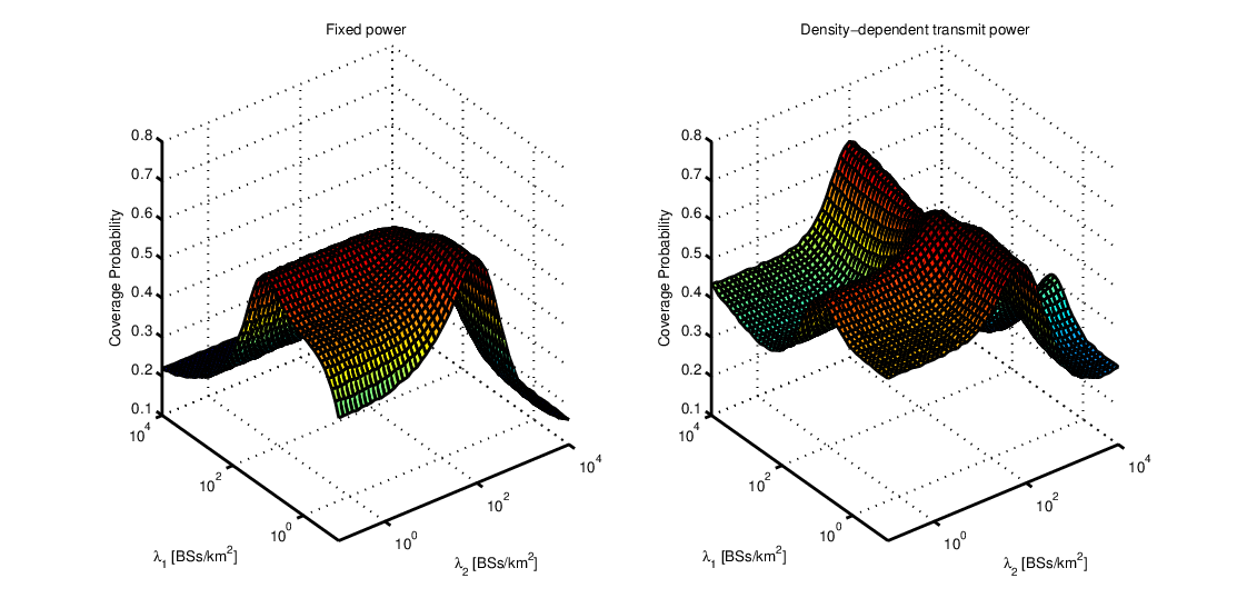
To have a full picture of the coverage probability with respect to λ1\lambda_{1} and λ2\lambda_{2}, present two 3D figures are presented in Fig. 5 and Fig. 6. In Fig. 5, we compare the MIRP and MARP association schemes based on the fixed transmit power. It is found that the coverage probability with the MIRP association scheme is always greater than that with the MARP association scheme as with former association scheme BSs can provide the maximum power all the time even though it is not practical in the real networks. In Fig. 6, coverage probability based on the fixed transmit power and density-dependent transmit power are illustrated, respectively. By utilizing a density-dependent transmit power, the coverage probability improves compared with the HetNets using \texorpdfstringa fixed transmit power.\texorpdfstring Besides, it is noted that the coverage probability using a density-dependent transmit power fluctuates with BS density as illustrated in Fig. 6 as well as in Fig. 2. It is because the imperfect power control used in Remark 1 which only depends on BS densities and an approximate equivalent coverage area, the 3D coverage probability appears more unique than that using a fixed transmit power.

V-B The PT and the EE
Refer to caption
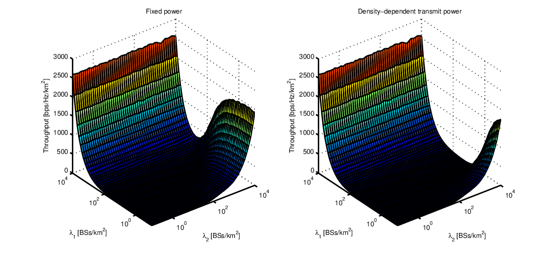
Figure 7: The PT vs. λ1\lambda_{1} and λ2\lambda_{2} based on the fixed transmit power and density-dependent transmit power.
Refer to caption
Figure 8: The EE vs. λ1\lambda_{1} and λ2\lambda_{2} based on the fixed transmit power and density-dependent transmit power in scenario S1.
Refer to caption
Figure 9: The EE vs. λ1\lambda_{1} and λ2\lambda_{2} based on the fixed transmit power and density-dependent transmit power in scenario S2.

In this subsection, two typical energy consumption scenarios are considered, i.e., practical power consumption and ideal power consumption, denoted by S1 and S2. Recall that the definition of the EE in Eq. (9) have parameters {ak}\left\{a_{k}\right\} and {bk}\left\{b_{k}\right\}, thus we define S1 as the HetNets which are configured with {a1=22.6,a2=5.5,b1=414.2,b2=32}\left\{a_{1}=22.6,a_{2}=5.5,b_{1}=414.2,b_{2}=32\right\} [29] and S2 configured with {a1=1,a2=1,b1=0,b2=0}\left\{a_{1}=1,a_{2}=1,b_{1}=0,b_{2}=0\right\}, respectively. Note that S2 accounts for the HetNets with perfect power amplifier and ignoring the static power consumed by signal processing, battery backup\texorpdfstring, and cooling, etc. In other words, in S2 only radiated power is considered. It is observed that λ1\lambda_{1} has a greater impact on the PT than λ2\lambda_{2} in Fig. 7. However, a larger λ1\lambda_{1} can not always provide a better EE as illustrated in Fig. 8 and Fig. 9. Therefore, there should exist a tradeoff among coverage probability, the PT and the EE, which is \texorpdfstringrevealed in the following subsection.

V-C Optimal Deployment Solutions

Refer to caption
Figure 10: 𝐎𝐏𝟏\mathbf{OP1}: The Maximum coverage probability vs. PmaxP^{\max} in scenarios \texorpdfstringS1, S2 and S3 (S3: {a1=10.3,a2=5.5,b1=156.2,b2=32}\left\{a_{1}=10.3,a_{2}=5.5,b_{1}=156.2,b_{2}=32\right\}).
Refer to caption
Figure 11: 𝐎𝐏𝟏\mathbf{OP1}: The optimal λ2\lambda_{2} vs. PmaxP^{\max} in scenarios \texorpdfstringS1, S2 and S3 (S3: {a1=10.3,a2=5.5,b1=156.2,b2=32}\left\{a_{1}=10.3,a_{2}=5.5,b_{1}=156.2,b_{2}=32\right\}).
Refer to caption
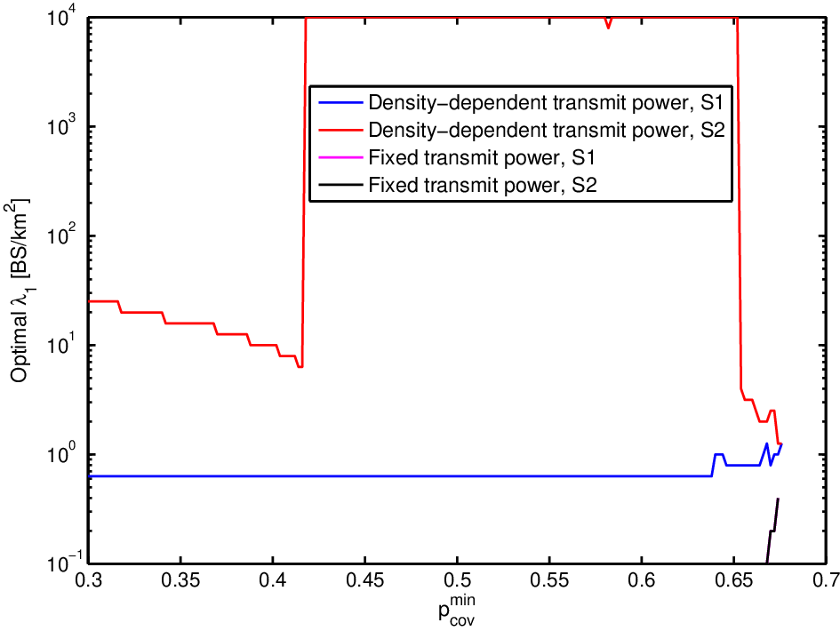
Figure 12: 𝐎𝐏𝟏\mathbf{OP1}: The optimal λ1\lambda_{1} vs. PmaxP^{\max} in scenarios \texorpdfstringS1, S2 and S3 (S3: {a1=10.3,a2=5.5,b1=156.2,b2=32}\left\{a_{1}=10.3,a_{2}=5.5,b_{1}=156.2,b_{2}=32\right\}).

In this subsection, present the optimal deployment solutions for 𝐎𝐏𝟏\mathbf{OP1} and 𝐎𝐏𝟐\mathbf{OP2} are presented. Regarding 𝐎𝐏𝟏\mathbf{OP1}, Fig. 10, Fig. 11 and Fig. 12 offer the optimal coverage probability, the optimal λ2\lambda_{2} and the optimal λ1\lambda_{1} with respect to PmaxP^{\max}, respectively. \texorpdfstringFrom Fig. 10, we conclude that the maximum coverage probability increases with the increase of PmaxP^{\max} and finally becomes invariant with PmaxP^{\max}. The reason behind this is that a larger PmaxP^{\max} provides more flexible BS deployment choice which will finally approach the optimal BS deployment without the constrain\texorpdfstringt of power consumption. Besides, the maximum coverage probability of HetNets with a density-dependent transmit power is more sensitive than that with a fixed transmit power. By comparison, the maximum coverage probability in S2 is superior to that in S1 when PmaxP^{\max} is small and inferior to that in S1 when PmaxP^{\max} becomes large. The optimal λ2\lambda_{2} in S1 grows up to a certain value with the increase of PmaxP^{\max}, after which the optimal λ2\lambda_{2} reaches its saturation, as illustrated in Fig. 11. While in S2, the optimal λ2\lambda_{2} has an opposite tendency compared with that in S1. It is because\texorpdfstring, in S1, static power consumption takes up most of the total power, especially for the macrocell BSs. Therefore, deploying more small cell BSs can save much more energy. If ignoring the static power consumption, i.e., S2 is considered, every single macrocell BS can provide a better coverage performance than every single small cell BS, thus more macrocell BSs should be deployed in this scenario as shown in Fig. 12.

Refer to caption
Figure 13: 𝐎𝐏𝟐\mathbf{OP2}: The maximum EE vs. pcovminp_{\textrm{cov}}^{\min} in scenarios S1 and S2.
Refer to caption
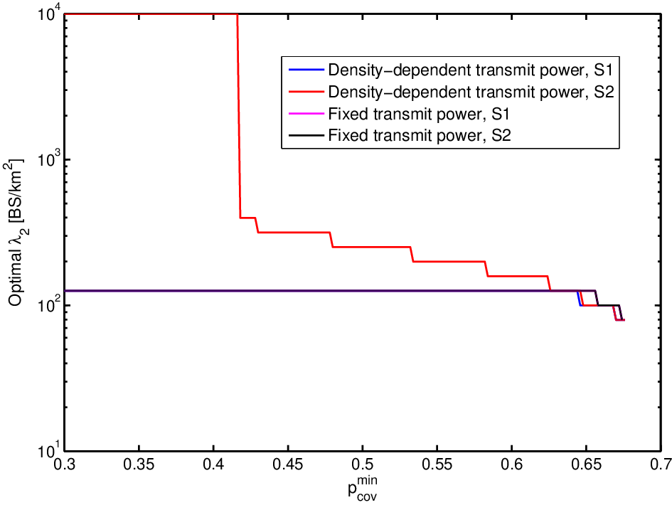
Figure 14: 𝐎𝐏𝟐\mathbf{OP2}: The optimal λ2\lambda_{2} vs. pcovminp_{\textrm{cov}}^{\min} in scenarios S1 and S2.
Refer to caption
Figure 15: 𝐎𝐏𝟐\mathbf{OP2}: The optimal λ1\lambda_{1} vs. pcovminp_{\textrm{cov}}^{\min} in scenarios S1 and S2.

Regarding 𝐎𝐏𝟐\mathbf{OP2}, Fig. 13, Fig. 14 and Fig. 15 present the maximum EE, the optimal λ2\lambda_{2} and λ1\lambda_{1}, respectively. It is observed in Fig. 13 that the maximum EE is a decreasing function with respect to pcovminp_{\textrm{cov}}^{\min}. It is because a smaller pcovminp_{\textrm{cov}}^{\min} corresponds to a less constrain\texorpdfstringt to the network deployment, as a result choosing proper BS densities becomes much more feasible for mobile operators. The tendency of the red curve, i.e., utilizing a density-dependent transmit power in S2, is greatly different from the rest. It is because the corresponding curve of the EE vs. λ1\lambda_{1} and λ2\lambda_{2} as illustrated in Fig. 8 and Fig. 9 is different from that of the rest. \texorpdfstringIt is also noted that the optimal EE is not strictly related to pcovminp_{\textrm{cov}}^{\min}, e.g., when 0.43≤pcovmin≤0.480.43\leq p_{\textrm{cov}}^{\min}\leq 0.48 for the red curve and when 0.30≤pcovmin≤0.6560.30\leq p_{\textrm{cov}}^{\min}\leq 0.656 for the black curve, the optimal EE remains the same. It is because, in these regimes, the optimal λ1\lambda_{1} and λ2\lambda_{2} can guarantee the coverage probability is greater a bit more than the threshold, i.e., pcovminp_{\textrm{cov}}^{\min}. To be specific, when we deploy λ1=104​ BS/km2\lambda_{1}=10^{4}\textrm{ BS/k$m^{2}$} and λ2=316.2​ BS/km2\lambda_{2}=316.2\textrm{ BS/k$m^{2}$}, the coverage probability is 0.48. And if we set pcovmin=0.43p_{\textrm{cov}}^{\min}=0.43, the deployment of BSs, i.e., λ1=104​ BS/km2\lambda_{1}=10^{4}\textrm{ BS/k$m^{2}$} and λ2=316.2​ BS/km2\lambda_{2}=316.2\textrm{ BS/k$m^{2}$}, can guarantee the minimal coverage probability thus keeps the optimal EE the same. Moreover, when pcovminp_{\textrm{cov}}^{\min} is greater than a certain value, e.g., 0.6762 of the red curve, there is no feasible solution to achieve the optimal EE as the QoS of the network, i.e., the coverage probability, can not be guaranteed. The optimal λ2\lambda_{2} is also a decreasing function with respect to pcovminp_{\textrm{cov}}^{\min} in Fig. 14. In Fig. 15, when pcovminp_{\textrm{cov}}^{\min} is small, the network is not constrain\texorpdfstringted by the coverage performance and deploying more small cell BSs can achieve a better EE. While when pcovminp_{\textrm{cov}}^{\min} is larger, mobile operators have to deploy more macrocell BSs to guarantee the network coverage performance, which results in a worse EE. The tendency of the red curve in Fig. 15 is rather different \texorpdfstringfrom others. When pcovminp_{\textrm{cov}}^{\min} is small, the optimal λ1\lambda_{1} decreases with the increase of pcovminp_{\textrm{cov}}^{\min}, then a “flip-flop phenomenon” appears, i.e., the optimal λ1\lambda_{1} jumps to a high value to guarantee the coverage performance and then decreases to a low value to achieve high EE.\texorpdfstring Besides, comparing Fig. 14 and Fig. 15, it is found that to achieve the optimal EE, an adjustment of λ1\lambda_{1} is needed when pcovminp_{\textrm{cov}}^{\min} is small, i.e., 0.30≤pcovmin≤0.420.30\leq p_{\textrm{cov}}^{\min}\leq 0.42, while λ2\lambda_{2} may keep the same; an adjustment of λ2\lambda_{2} is needed when pcovminp_{\textrm{cov}}^{\min} is medium, i.e., 0.42≤pcovmin≤0.650.42\leq p_{\textrm{cov}}^{\min}\leq 0.65, while λ1\lambda_{1} may keep the same; an adjustment of λ1\lambda_{1} as well as λ2\lambda_{2} is needed when pcovminp_{\textrm{cov}}^{\min} is large, i.e., pcovmin≥0.65p_{\textrm{cov}}^{\min}\geq 0.65.

VI Conclusions and Future Work

In this paper, we investigated network performance of downlink ultra-dense HetNets and study the maximum energy-efficient BS deployment incorporating both NLoS and LoS transmissions. Through analysis, we found that the coverage probability with the MIRP association scheme is better than that with the MARP association scheme and by utilizing a density-dependent transmit power, the coverage probability improves when densities of macrocell BSs and small cell BSs are sparse or medium compared with the HetNets using the fixed transmit power. Moreover, we formulated two optimization problems to achieve the maximum energy-efficient deployment solution with certain minimum service criteria. Simulation results show that there are tradeoffs among the coverage probability, the total power consumption and the EE. In detail, the maximum coverage probability with ideal power consumption is superior to that with practical power consumption when the total power constrain\texorpdfstringt is small and inferior to that with practical power consumption when the total power constrain\texorpdfstringt becomes large. Furthermore, the maximum EE is a decreasing function with respect to the coverage probability constrain\texorpdfstringt. In our future work, networks with idle mode capability and multiple-antennas are also worth further studying.

Appendix A: Proof of Theorem 1

Proof:

The coverage probability in a KK-tier HetNet with the MIRP association scheme is defined as follows

pcovMIRP({λk},{Tk},{BkU})=Pr[∪k∈𝒦,𝑿k,o∈ΦkSINRk(‖𝑿k,o‖)>Tk].p_{\textrm{cov}}^{\textrm{MIRP}}\left(\left\{\lambda_{k}\right\},\left\{T_{k}\right\},\left\{B_{k}^{\textrm{U}}\right\}\right)=\Pr\Bigl[\underset{k\in\mathcal{K},\boldsymbol{X}_{k,o}\in\Phi_{k}}{\cup}\textrm{SINR}_{k}\left(\left\|\boldsymbol{X}_{k,o}\right\|\right)>T_{k}\Bigr]. (34)

As we consider both NLoS and LoS transmissions, pcovMIRP​({λk},{Tk},{BkU})p_{\textrm{cov}}^{\textrm{MIRP}}\left(\left\{\lambda_{k}\right\},\left\{T_{k}\right\},\left\{B_{k}^{\textrm{U}}\right\}\right) can be further expressed by\texorpdfstring

pcovMIRP({λk},{Tk},{BkU})=Pr[∪k∈𝒦,𝑿k,o∈ΦkSINRk(‖𝑿k,o‖)>Tk]\displaystyle\quad\,p_{\textrm{cov}}^{\textrm{MIRP}}\left(\left\{\lambda_{k}\right\},\left\{T_{k}\right\},\left\{B_{k}^{\textrm{U}}\right\}\right)=\Pr\Bigl[\underset{k\in\mathcal{K},\boldsymbol{X}_{k,o}\in\Phi_{k}}{\cup}\textrm{SINR}_{k}\left(\left\|\boldsymbol{X}_{k,o}\right\|\right)>T_{k}\Bigr]
=𝔼⁡[𝕀⁡(∪k∈𝒦,𝑿k,o∈Φk​SINRk​(‖𝑿k,o‖)>Tk)]\displaystyle=\mathbb{E}\left[\mathbb{I}\left(\underset{k\in\mathcal{K},\boldsymbol{X}_{k,o}\in\Phi_{k}}{\cup}\textrm{SINR}_{k}\left(\left\|\boldsymbol{X}_{k,o}\right\|\right)>T_{k}\right)\right]
=∑𝔼⁡{∑𝑿k,o∈ΦkNL​[𝕀⁡(SINRkNL​(‖𝑿k,o‖)>Tk)]}⏟I\displaystyle=\underset{\textrm{I}}{\underbrace{\mathrel{{\mathop{\sum}\limits}}\mathbb{E}\Bigl\{\underset{\boldsymbol{X}_{k,o}\in\Phi_{k}^{\textrm{NL}}}{\sum}\left[\mathbb{I}\left(\textrm{SINR}_{k}^{\textrm{NL}}\left(\left\|\boldsymbol{X}_{k,o}\right\|\right)>T_{k}\right)\right]\Bigr\}}}
+∑𝔼⁡{∑𝑿k,o∈ΦkL​[𝕀⁡(SINRkL​(‖𝑿k,o‖)>Tk)]}⏟II,\displaystyle\quad\,+\underset{\textrm{II}}{\underbrace{\mathrel{{\mathop{\sum}\limits}}\mathbb{E}\Bigl\{\underset{\boldsymbol{X}_{k,o}\in\Phi_{k}^{\textrm{L}}}{\sum}\left[\mathbb{I}\left(\textrm{SINR}_{k}^{\textrm{L}}\left(\left\|\boldsymbol{X}_{k,o}\right\|\right)>T_{k}\right)\right]\Bigr\}}}, (35)

where 𝕀⁡(⋅)\mathbb{I}\left(\cdot\right) is the indicator function, (a)\left(a\right) follows from [40, Lemma 1] under the assumption that Tk⩾1​∀kT_{k}\geqslant 1\forall k and the independence between ΦkNL\Phi_{k}^{\textrm{NL}} and ΦkL\Phi_{k}^{\textrm{L}}, Part I and II in Eq. (35) can be comprehended as the probability that the typical MU is covered by NLoS BSs and LoS BSs, respectively.

For Part I in Eq. (35), we have

∑𝔼⁡{∑𝑿k,o∈ΦkNL​[𝕀⁡(SINRkNL​(‖𝑿k,o‖)>Tk)]}​=(a)∑𝔼⁡{∑Rk,oNL¯∈ΦkNL¯​[𝕀⁡(SINRkNL​(Rk,oNL¯)>Tk)]}\displaystyle\quad\,\mathrel{{\mathop{\sum}\limits}}\mathbb{E}\Bigl\{\underset{\boldsymbol{X}_{k,o}\in\Phi_{k}^{\textrm{NL}}}{\sum}\left[\mathbb{I}\left(\textrm{SINR}_{k}^{\textrm{NL}}\left(\left\|\boldsymbol{X}_{k,o}\right\|\right)>T_{k}\right)\right]\Bigr\}\overset{\left(a\right)}{=}\mathrel{{\mathop{\sum}\limits}}\mathbb{E}\Bigl\{\underset{\overline{R_{k,o}^{\textrm{NL}}}\in\overline{\Phi_{k}^{\textrm{NL}}}}{\sum}\left[\mathbb{I}\left(\textrm{SINR}_{k}^{\textrm{NL}}\left(\overline{R_{k,o}^{\textrm{NL}}}\right)>T_{k}\right)\right]\Bigr\}
=(b)∑∫r=0∞Pr[hkNL​r−αkNL∑∑i:rj,i∈ΦjNL^hjNLrj,i−αjNL+∑∑i:rj,i∈ΦjL¯hjLrj,i−αjL+η>Tk]λkNL(r)dr\displaystyle\overset{\left(b\right)}{=}\mathrel{{\mathop{\sum}\limits}}\int_{r=0}^{\infty}\Pr\Biggl[\frac{h_{k}^{\textrm{NL}}r^{-\alpha_{k}^{\textrm{NL}}}}{\mathrel{{\mathop{\sum}\limits}}\underset{i:r_{j,i}\in\widehat{\Phi_{j}^{\textrm{NL}}}}{\sum}h_{j}^{\textrm{NL}}r_{j,i}^{-\alpha_{j}^{\textrm{NL}}}+\mathrel{{\mathop{\sum}\limits}}\underset{i:r_{j,i}\in\overline{\Phi_{j}^{\textrm{L}}}}{\sum}h_{j}^{\textrm{L}}r_{j,i}^{-\alpha_{j}^{\textrm{L}}}+\eta}>T_{k}\Biggr]\lambda_{k}^{\textrm{NL}}\left(r\right)\textrm{d}r
=(c)∑∫r=0∞Pr[hkNL​r−αkNL∑IjNL+∑IjL+η>Tk]λkNL(r)dr\displaystyle\overset{\left(c\right)}{=}\mathrel{{\mathop{\sum}\limits}}\int_{r=0}^{\infty}\Pr\Biggl[\frac{h_{k}^{\textrm{NL}}r^{-\alpha_{k}^{\textrm{NL}}}}{\mathrel{{\mathop{\sum}\limits}}I_{j}^{\textrm{NL}}+\mathrel{{\mathop{\sum}\limits}}I_{j}^{\textrm{L}}+\eta}>T_{k}\Biggr]\lambda_{k}^{\textrm{NL}}\left(r\right)\textrm{d}r
=(d)∑∫r=0∞e−Tk​η​rαkNL​λkNL​(r)∏[ℒIjNLMIRP​(Tk​rαkNL)​ℒIjLMIRP​(Tk​rαkNL)]​d​r,\displaystyle\overset{\left(d\right)}{=}\mathrel{{\mathop{\sum}\limits}}\int_{r=0}^{\infty}e^{-T_{k}\eta r^{\alpha_{k}^{\textrm{NL}}}}\lambda_{k}^{\textrm{NL}}\left(r\right)\mathrel{{\mathop{\prod}\limits}}\left[\mathcal{L}_{I_{j}^{\textrm{NL}}}^{\textrm{MIRP}}\left(T_{k}r^{\alpha_{k}^{\textrm{NL}}}\right)\mathcal{L}_{I_{j}^{\textrm{L}}}^{\textrm{MIRP}}\left(T_{k}r^{\alpha_{k}^{\textrm{NL}}}\right)\right]\textrm{d}r, (36)

where (a)\left(a\right) is due to the transformation from ΦkNL\Phi_{k}^{\textrm{NL}} to ΦkNL¯\overline{\Phi_{k}^{\textrm{NL}}}, (b)\left(b\right) follows from Campbell theorem [20] and variable substitution, i.e., Rk,oNL¯→r\overline{R_{k,o}^{\textrm{NL}}}\rightarrow r, in (c)\left(c\right) IjNL=def∑i:rj,i∈ΦjNL¯′hiNLrj,i−αjNLI_{j}^{\textrm{NL}}\overset{\textrm{def}}{=}\underset{i:r_{j,i}\in\overline{\Phi_{j}^{\textrm{NL}}}^{\prime}}{\sum}h_{i}^{\textrm{NL}}r_{j,i}^{-\alpha_{j}^{\textrm{NL}}} and IjL=def∑i:rj,i∈ΦjNL¯hiLrj,i−αjLI_{j}^{\textrm{L}}\overset{\textrm{def}}{=}\underset{i:r_{j,i}\in\overline{\Phi_{j}^{\textrm{NL}}}}{\sum}h_{i}^{\textrm{L}}r_{j,i}^{-\alpha_{j}^{\textrm{L}}} are the aggregate interference from NLoS BSs and LoS BSs in the jj-th tier, respectively, where ΦjNL^=ΦjNL¯∖(0,Rk,oNL¯]\widehat{\Phi_{j}^{\textrm{NL}}}=\overline{\Phi_{j}^{\textrm{NL}}}\setminus\left(0,\overline{R_{k,o}^{\textrm{NL}}}\right], (d)\left(d\right) is due to hkNL∼exp⁡(1)h_{k}^{\textrm{NL}}\sim\exp\left(1\right), ℒIjNLMIRP​(s)\mathcal{L}_{I_{j}^{\textrm{NL}}}^{\textrm{MIRP}}\left(s\right) and ℒIjLMIRP​(s)\mathcal{L}_{I_{j}^{\textrm{L}}}^{\textrm{MIRP}}\left(s\right) denote the Laplace transform of IjNLI_{j}^{\textrm{NL}} and IjLI_{j}^{\textrm{L}} evaluated at ss with the MIRP association scheme, respectively. Using the definition of Laplace transform, we derive ℒIjNLMIRP​(s)\mathcal{L}_{I_{j}^{\textrm{NL}}}^{\textrm{MIRP}}\left(s\right) as follows

ℒIjNLMIRP(s)=𝔼IjNL[e−s​IjNL]=(a)𝔼ΦjNL¯[∏i:rj,i∈ΦjNL^𝔼hNL(e−s​hNL​rj,i−αjNL)]\displaystyle\quad\,\mathcal{L}_{I_{j}^{\textrm{NL}}}^{\textrm{MIRP}}\left(s\right)=\mathbb{E}_{I_{j}^{\textrm{NL}}}\left[e^{-sI_{j}^{\textrm{NL}}}\right]\overset{\left(a\right)}{=}\mathbb{E}_{\overline{\Phi_{j}^{\textrm{NL}}}}\biggl[\underset{i:r_{j,i}\in\widehat{\Phi_{j}^{\textrm{NL}}}}{\prod}\mathbb{E}_{h^{\textrm{NL}}}\left(e^{-sh^{\textrm{NL}}r_{j,i}^{-\alpha_{j}^{\textrm{NL}}}}\right)\biggr]
=𝔼ΦjNL¯[∏i:rj,i∈ΦjNL^11+s​rj,i−αjNL]=(b)exp[∫y=0∞(11+s​y−αjNL−1)λjNL(y)dy]\displaystyle=\mathbb{E}_{\overline{\Phi_{j}^{\textrm{NL}}}}\biggl[\underset{i:r_{j,i}\in\widehat{\Phi_{j}^{\textrm{NL}}}}{\prod}\frac{1}{1+sr_{j,i}^{-\alpha_{j}^{\textrm{NL}}}}\biggr]\overset{\left(b\right)}{=}\exp\biggl[\int_{y=0}^{\infty}\left(\frac{1}{1+sy^{-\alpha_{j}^{\textrm{NL}}}}-1\right)\lambda_{j}^{\textrm{NL}}\left(y\right)\textrm{d}y\biggr]
=exp[−∫y=0∞λjNL​(y)1+yαjNL/sdy]=exp[−s1/αjNL∫y=0∞λjNL​(y​s1/αjNL)1+yαjNLdy],\displaystyle=\exp\biggl[-\int_{y=0}^{\infty}\frac{\lambda_{j}^{\textrm{NL}}\left(y\right)}{1+y^{\alpha_{j}^{\textrm{NL}}}/s}\textrm{d}y\biggr]=\exp\biggl[-s^{1/\alpha_{j}^{\textrm{NL}}}\int_{y=0}^{\infty}\frac{\lambda_{j}^{\textrm{NL}}\left(ys^{1/\alpha_{j}^{\textrm{NL}}}\right)}{1+y^{\alpha_{j}^{\textrm{NL}}}}\textrm{d}y\biggr], (37)

where (a)\left(a\right) follows from the independence between the fading random variables (RVs), i.e., hjNLh_{j}^{\textrm{NL}}, (b)\left(b\right) follows from probability generating functional (PGFL) of PPP [20].

Similarly, ℒIjLMIRP​(s)\mathcal{L}_{I_{j}^{\textrm{L}}}^{\textrm{MIRP}}\left(s\right) is obtained as follows

ℒIjLMIRP(s)=𝔼IjL[e−s​IjL]=exp[−∫y=0∞λjL​(y)1+yαjL/sdy]\displaystyle\quad\,\mathcal{L}_{I_{j}^{\textrm{L}}}^{\textrm{MIRP}}\left(s\right)=\mathbb{E}_{I_{j}^{\textrm{L}}}\left[e^{-sI_{j}^{\textrm{L}}}\right]=\exp\biggl[-\int_{y=0}^{\infty}\frac{\lambda_{j}^{\textrm{L}}\left(y\right)}{1+y^{\alpha_{j}^{\textrm{L}}}/s}\textrm{d}y\biggr]
=exp[−s1/αjL∫y=0∞λjL​(y​s1/αjL)1+yαjLdy],\displaystyle=\exp\biggl[-s^{1/\alpha_{j}^{\textrm{L}}}\int_{y=0}^{\infty}\frac{\lambda_{j}^{\textrm{L}}\left(ys^{1/\alpha_{j}^{\textrm{L}}}\right)}{1+y^{\alpha_{j}^{\textrm{L}}}}\textrm{d}y\biggr], (38)

Using a similar approach compared with Part I, Part II can also be easily obtained as follows

∑𝔼⁡{∑𝑿k,o∈ΦkL​[𝕀⁡(SINRL​(‖𝑿k,o‖)>Tk)]}\displaystyle\quad\,\mathrel{{\mathop{\sum}\limits}}\mathbb{E}\left\{\underset{\boldsymbol{X}_{k,o}\in\Phi_{k}^{\textrm{L}}}{\sum}\left[\mathbb{I}\left(\textrm{SINR}^{\textrm{L}}\left(\left\|\boldsymbol{X}_{k,o}\right\|\right)>T_{k}\right)\right]\right\}
=∑∫t=0∞e−Tk​η​rαkLλkL(r)∏[ℒIjNLMIRP(TkrαkL)ℒIjLMIRP(TkrαkL)]dr,\displaystyle=\mathrel{{\mathop{\sum}\limits}}\int_{t=0}^{\infty}e^{-T_{k}\eta r^{\alpha_{k}^{\textrm{L}}}}\lambda_{k}^{\textrm{L}}\left(r\right)\mathrel{{\mathop{\prod}\limits}}\left[\mathcal{L}_{I_{j}^{\textrm{NL}}}^{\textrm{MIRP}}\left(T_{k}r^{\alpha_{k}^{\textrm{L}}}\right)\mathcal{L}_{I_{j}^{\textrm{L}}}^{\textrm{MIRP}}\left(T_{k}r^{\alpha_{k}^{\textrm{L}}}\right)\right]\textrm{d}r, (39)

where ℒIjNLMIRP​(s)\mathcal{L}_{I_{j}^{\textrm{NL}}}^{\textrm{MIRP}}\left(s\right) and ℒIjLMIRP​(s)\mathcal{L}_{I_{j}^{\textrm{L}}}^{\textrm{MIRP}}\left(s\right) are defined in Eq. (37) and Eq. (38), respectively. Then, the proof is completed. ∎

Appendix B: Proof of Theorem 2

Using the law of total probability, we can calculate coverage probability pcovMARP​({λk},{Tk},{BkU})p_{\textrm{cov}}^{\textrm{MARP}}\left(\left\{\lambda_{k}\right\},\left\{T_{k}\right\},\left\{B_{k}^{\textrm{U}}\right\}\right) as

pcovMARP​({λk},{Tk},{BkU})=∑pkNL​({λkNL},{Tk},{BkNL})+∑pkL​({λkL},{Tk},{BkL}),p_{\textrm{cov}}^{\textrm{MARP}}\left(\left\{\lambda_{k}\right\},\left\{T_{k}\right\},\left\{B_{k}^{\textrm{U}}\right\}\right)=\mathrel{{\mathop{\sum}\limits}}p_{k}^{\textrm{NL}}\left(\left\{\lambda_{k}^{\textrm{NL}}\right\},\left\{T_{k}\right\},\left\{B_{k}^{\textrm{NL}}\right\}\right)+\mathrel{{\mathop{\sum}\limits}}p_{k}^{\textrm{L}}\left(\left\{\lambda_{k}^{\textrm{L}}\right\},\left\{T_{k}\right\},\left\{B_{k}^{\textrm{L}}\right\}\right), (40)

where the first part and the second part on the right side of the equation denote the conditional coverage probability that the typical MU is in the coverage of NLoS BSs and LoS\texorpdfstring BSs, respectively, by observing that the two events are disjoint. Given that the typical MU is served by a\texorpdfstringn NLoS BS and an the maximum average received power is denote by 𝒫kNL\mathcal{P}_{k}^{\textrm{NL}}, i.e., 𝒫kNL=max⁡(Pk.iNL)\mathcal{P}_{k}^{\textrm{NL}}=\max\left(P_{k.i}^{\textrm{NL}}\right). Then

pkNL​({λkNL},{Tk},{BkNL})\displaystyle\quad\,p_{k}^{\textrm{NL}}\left(\left\{\lambda_{k}^{\textrm{NL}}\right\},\left\{T_{k}\right\},\left\{B_{k}^{\textrm{NL}}\right\}\right)
=Pr[(SINRkNL>Tk)∩(∩j∈𝒦{𝒫kNL>𝒫jL},∩j∈𝒦∖k{𝒫kNL>𝒫jNL})∩𝒴kNL]\displaystyle=\Pr\biggl[\left(\textrm{SINR}_{k}^{\textrm{NL}}>T_{k}\right)\cap\left(\underset{j\in\mathcal{K}}{\cap}\left\{\mathcal{P}_{k}^{\textrm{NL}}>\mathcal{P}_{j}^{\textrm{L}}\right\},\underset{j\in\mathcal{K}\setminus k}{\cap}\left\{\mathcal{P}_{k}^{\textrm{NL}}>\mathcal{P}_{j}^{\textrm{NL}}\right\}\right)\cap\mathcal{Y}_{k}^{\textrm{NL}}\biggr]
=𝔼𝒴kNL{Pr[SINRkNL>Tk|(∩j∈𝒦{𝒫kNL>𝒫jL},∩j∈𝒦∖k{𝒫kNL>𝒫jNL})∩𝒴kNL]⏟II\displaystyle=\mathbb{E}_{\mathcal{Y}_{k}^{\textrm{NL}}}\biggl\{\underset{\textrm{II}}{\underbrace{\Pr\biggl[\textrm{SINR}_{k}^{\textrm{NL}}>T_{k}\left|\left(\underset{j\in\mathcal{K}}{\cap}\left\{\mathcal{P}_{k}^{\textrm{NL}}>\mathcal{P}_{j}^{\textrm{L}}\right\},\underset{j\in\mathcal{K}\setminus k}{\cap}\left\{\mathcal{P}_{k}^{\textrm{NL}}>\mathcal{P}_{j}^{\textrm{NL}}\right\}\right)\cap\mathcal{Y}_{k}^{\textrm{NL}}\right.\biggr]}}
×Pr[∩j∈𝒦{𝒫kNL>𝒫jL},∩j∈𝒦∖k{𝒫kNL>𝒫jNL}|𝒴kNL]⏟I},\displaystyle\quad\,\times\underset{\textrm{I}}{\underbrace{\Pr\biggl[\left.\underset{j\in\mathcal{K}}{\cap}\left\{\mathcal{P}_{k}^{\textrm{NL}}>\mathcal{P}_{j}^{\textrm{L}}\right\},\underset{j\in\mathcal{K}\setminus k}{\cap}\left\{\mathcal{P}_{k}^{\textrm{NL}}>\mathcal{P}_{j}^{\textrm{NL}}\right\}\right|\mathcal{Y}_{k}^{\textrm{NL}}\biggr]}}\biggr\}, (41)

where 𝒴kNL\mathcal{Y}_{k}^{\textrm{NL}} is the equivalent distance between the typical MU and the BS providing the maximum average received power to the typical MU in ΦkNL\Phi_{k}^{\textrm{NL}}, i.e., 𝒴kNL=arg⁡maxRk.iNL¯∈ΦkNL¯​(Rk.iNL¯)−αkNL\mathcal{Y}_{k}^{\textrm{NL}}=\underset{\overline{R_{k.i}^{\textrm{NL}}}\in\overline{\Phi_{k}^{\textrm{NL}}}}{\arg\max}\left(\overline{R_{k.i}^{\textrm{NL}}}\right)^{-\alpha_{k}^{\textrm{NL}}}, and also note that 𝒫kNL=(𝒴kNL)−αkNL\mathcal{P}_{k}^{\textrm{NL}}=\left(\mathcal{Y}_{k}^{\textrm{NL}}\right)^{-\alpha_{k}^{\textrm{NL}}}. For Part I,

Pr[∩j∈𝒦{𝒫kNL>𝒫jL},∩j∈𝒦∖k{𝒫kNL>𝒫jNL}|𝒴kNL]\displaystyle\quad\,\Pr\left[\left.\underset{j\in\mathcal{K}}{\cap}\left\{\mathcal{P}_{k}^{\textrm{NL}}>\mathcal{P}_{j}^{\textrm{L}}\right\},\underset{j\in\mathcal{K}\setminus k}{\cap}\left\{\mathcal{P}_{k}^{\textrm{NL}}>\mathcal{P}_{j}^{\textrm{NL}}\right\}\right|\mathcal{Y}_{k}^{\textrm{NL}}\right]
=∏j∈𝒦Pr[𝒫kNL>𝒫jL|𝒴kNL]∏j∈𝒦∖kPr[𝒫kNL>𝒫jNL|𝒴kNL]\displaystyle=\underset{j\in\mathcal{K}}{\prod}\Pr\left[\left.\mathcal{P}_{k}^{\textrm{NL}}>\mathcal{P}_{j}^{\textrm{L}}\right|\mathcal{Y}_{k}^{\textrm{NL}}\right]\underset{j\in\mathcal{K}\setminus k}{\prod}\Pr\left[\left.\mathcal{P}_{k}^{\textrm{NL}}>\mathcal{P}_{j}^{\textrm{NL}}\right|\mathcal{Y}_{k}^{\textrm{NL}}\right]
=∏j∈𝒦Pr[(𝒴kNL)−αkNL>(𝒴jL)−αjL|𝒴kNL]∏j∈𝒦∖kPr[(𝒴kNL)−αkNL>(𝒴jNL)−αjNL|𝒴kNL]\displaystyle=\underset{j\in\mathcal{K}}{\prod}\Pr\left[\left.\left(\mathcal{Y}_{k}^{\textrm{NL}}\right)^{-\alpha_{k}^{\textrm{NL}}}>\left(\mathcal{Y}_{j}^{\textrm{L}}\right)^{-\alpha_{j}^{\textrm{L}}}\right|\mathcal{Y}_{k}^{\textrm{NL}}\right]\underset{j\in\mathcal{K}\setminus k}{\prod}\Pr\left[\left.\left(\mathcal{Y}_{k}^{\textrm{NL}}\right)^{-\alpha_{k}^{\textrm{NL}}}>\left(\mathcal{Y}_{j}^{\textrm{NL}}\right)^{-\alpha_{j}^{\textrm{NL}}}\right|\mathcal{Y}_{k}^{\textrm{NL}}\right]
=∏j∈𝒦Pr[𝒴jL>(𝒴kNL)αkNL/αjL|𝒴kNL]∏j∈𝒦∖kPr[𝒴jNL>(𝒴kNL)αkNL/αjNL|𝒴kNL]\displaystyle=\underset{j\in\mathcal{K}}{\prod}\Pr\left[\left.\mathcal{Y}_{j}^{\textrm{L}}>\left(\mathcal{Y}_{k}^{\textrm{NL}}\right)^{\alpha_{k}^{\textrm{NL}}/\alpha_{j}^{\textrm{L}}}\right|\mathcal{Y}_{k}^{\textrm{NL}}\right]\underset{j\in\mathcal{K}\setminus k}{\prod}\Pr\left[\left.\mathcal{Y}_{j}^{\textrm{NL}}>\left(\mathcal{Y}_{k}^{\textrm{NL}}\right)^{\alpha_{k}^{\textrm{NL}}/\alpha_{j}^{\textrm{NL}}}\right|\mathcal{Y}_{k}^{\textrm{NL}}\right]
=(a)​∏j∈𝒦​exp⁡[−ΛjL​([0,(𝒴kNL)αkNL/αjL])]​∏j∈𝒦∖k​exp​[−ΛjNL​([0,(𝒴kNL)αkNL/αjNL])]\displaystyle\overset{\left(a\right)}{=}\underset{j\in\mathcal{K}}{\prod}\exp\left[-\Lambda_{j}^{\textrm{L}}\left(\left[0,\left(\mathcal{Y}_{k}^{\textrm{NL}}\right)^{\alpha_{k}^{\textrm{NL}}/\alpha_{j}^{\textrm{L}}}\right]\right)\right]\underset{j\in\mathcal{K}\setminus k}{\prod}\exp\left[-\Lambda_{j}^{\textrm{NL}}\left(\left[0,\left(\mathcal{Y}_{k}^{\textrm{NL}}\right)^{\alpha_{k}^{\textrm{NL}}/\alpha_{j}^{\textrm{NL}}}\right]\right)\right]
=exp⁡{−∑j∈𝒦​[ΛjL​([0,(𝒴kNL)αkNL/αjL])+ΛjNL​([0,(𝒴kNL)αkNL/αjNL])]+ΛkNL​([0,𝒴kNL])},\displaystyle=\exp\biggl\{-\underset{j\in\mathcal{K}}{\sum}\left[\Lambda_{j}^{\textrm{L}}\left(\left[0,\left(\mathcal{Y}_{k}^{\textrm{NL}}\right)^{\alpha_{k}^{\textrm{NL}}/\alpha_{j}^{\textrm{L}}}\right]\right)+\Lambda_{j}^{\textrm{NL}}\left(\left[0,\left(\mathcal{Y}_{k}^{\textrm{NL}}\right)^{\alpha_{k}^{\textrm{NL}}/\alpha_{j}^{\textrm{NL}}}\right]\right)\right]+\Lambda_{k}^{\textrm{NL}}\left(\left[0,\mathcal{Y}_{k}^{\textrm{NL}}\right]\right)\biggr\}, (42)

where 𝒴kL\mathcal{Y}_{k}^{\textrm{L}}, similar to the definition of 𝒴kNL\mathcal{Y}_{k}^{\textrm{NL}}, is the equivalent distance between the typical MU and the BS providing the maximum average received power to the typical MU in ΦkL\Phi_{k}^{\textrm{L}}, i.e., 𝒴kL=arg⁡maxRk,iL¯∈ΦkL¯​(Rk,iL¯)−αkL\mathcal{Y}_{k}^{\textrm{L}}=\underset{\overline{R_{k,i}^{\textrm{L}}}\in\overline{\Phi_{k}^{\textrm{L}}}}{\arg\max}\left(\overline{R_{k,i}^{\textrm{L}}}\right)^{-\alpha_{k}^{\textrm{L}}}, and also note that 𝒫kL=(𝒴kL)−αkL\mathcal{P}_{k}^{\textrm{L}}=\left(\mathcal{Y}_{k}^{\textrm{L}}\right)^{-\alpha_{k}^{\textrm{L}}}, and (a)\left(a\right) follows from the void probability of a PPP.

For Part II, we know that SINRkNL=hkNL​𝒫kNL∑IjNL+∑IjL+η\textrm{SINR}_{k}^{\textrm{NL}}=\frac{h_{k}^{\textrm{NL}}\mathcal{P}_{k}^{\textrm{NL}}}{\mathrel{{\mathop{\sum}\limits}}I_{j}^{\textrm{NL}}+\mathrel{{\mathop{\sum}\limits}}I_{j}^{\textrm{L}}+\eta}. The conditional coverage probability can be derived as follows

Pr[SINRkNL>Tk|(∩j∈𝒦{𝒫kNL>𝒫jL},∩j∈𝒦∖k{𝒫kNL>𝒫jNL})∩𝒴kNL]\displaystyle\quad\,\Pr\biggl[\textrm{SINR}_{k}^{\textrm{NL}}>T_{k}\left|\left(\underset{j\in\mathcal{K}}{\cap}\left\{\mathcal{P}_{k}^{\textrm{NL}}>\mathcal{P}_{j}^{\textrm{L}}\right\},\underset{j\in\mathcal{K}\setminus k}{\cap}\left\{\mathcal{P}_{k}^{\textrm{NL}}>\mathcal{P}_{j}^{\textrm{NL}}\right\}\right)\cap\mathcal{Y}_{k}^{\textrm{NL}}\right.\biggr]
=(a)​Pr⁡[hkNL​(𝒴kNL)−αkNL∑IjNL+∑IjL+η>Tk|E]\displaystyle\overset{\left(a\right)}{=}\Pr\biggl[\frac{h_{k}^{\textrm{NL}}\left(\mathcal{Y}_{k}^{\textrm{NL}}\right)^{-\alpha_{k}^{\textrm{NL}}}}{\mathrel{{\mathop{\sum}\limits}}I_{j}^{\textrm{NL}}+\mathrel{{\mathop{\sum}\limits}}I_{j}^{\textrm{L}}+\eta}>T_{k}\biggl|\textrm{E}\biggr]
=Pr[hkNL>Tk(𝒴kNL)αkNL(∑IjNL+∑IjL+η)|E]\displaystyle=\Pr\biggl[h_{k}^{\textrm{NL}}>T_{k}\left(\mathcal{Y}_{k}^{\textrm{NL}}\right)^{\alpha_{k}^{\textrm{NL}}}\left(\mathrel{{\mathop{\sum}\limits}}I_{j}^{\textrm{NL}}+\mathrel{{\mathop{\sum}\limits}}I_{j}^{\textrm{L}}+\eta\right)\biggl|\textrm{E}\biggr]
=(b)​e−Tk​η​rαkNL∏[ℒIjNLMARP1​(Tk​rαkNL)​ℒIjLMARP1​(Tk​rαkNL)],\displaystyle\overset{\left(b\right)}{=}e^{-T_{k}\eta r^{\alpha_{k}^{\textrm{NL}}}}\mathrel{{\mathop{\prod}\limits}}\left[\mathcal{L}_{I_{j}^{\textrm{NL}}}^{\textrm{MARP1}}\left(T_{k}r^{\alpha_{k}^{\textrm{NL}}}\right)\mathcal{L}_{I_{j}^{\textrm{L}}}^{\textrm{MARP1}}\left(T_{k}r^{\alpha_{k}^{\textrm{NL}}}\right)\right], (43)

where in (a)\left(a\right) event E=def(∩j∈𝒦{𝒫kNL>𝒫jL},∩j∈𝒦∖k{𝒫kNL>𝒫jNL})∩𝒴kNL\textrm{E}\overset{\textrm{def}}{=}\left(\underset{j\in\mathcal{K}}{\cap}\left\{\mathcal{P}_{k}^{\textrm{NL}}>\mathcal{P}_{j}^{\textrm{L}}\right\},\underset{j\in\mathcal{K}\setminus k}{\cap}\left\{\mathcal{P}_{k}^{\textrm{NL}}>\mathcal{P}_{j}^{\textrm{NL}}\right\}\right)\cap\mathcal{Y}_{k}^{\textrm{NL}}, (b)\left(b\right) follows from hkNL∼exp⁡(1)h_{k}^{\textrm{NL}}\sim\exp\left(1\right) and variable substitution, i.e., 𝒴kNL→r\mathcal{Y}_{k}^{\textrm{NL}}\rightarrow r, ℒIjNLave​(s)\mathcal{L}_{I_{j}^{\textrm{NL}}}^{\textrm{ave}}\left(s\right) and ℒIjLave​(s)\mathcal{L}_{I_{j}^{\textrm{L}}}^{\textrm{ave}}\left(s\right) denote the Laplace transform of IjNLI_{j}^{\textrm{NL}} and IjLI_{j}^{\textrm{L}} evaluated at ss with the MARP association scheme, respectively. Like Appendix A, we derive ℒIjNLMARP​(s)\mathcal{L}_{I_{j}^{\textrm{NL}}}^{\textrm{MARP}}\left(s\right) as follows

ℒIjNLMARP1(s)=𝔼IjNL[e−s​IjNL]=𝔼ΦjNL¯[∏i:rj,i∈ΦjNL^𝔼hNL(e−s​hNL​rj,i−αjNL)]\displaystyle\quad\,\mathcal{L}_{I_{j}^{\textrm{NL}}}^{\textrm{MARP1}}\left(s\right)=\mathbb{E}_{I_{j}^{\textrm{NL}}}\left[e^{-sI_{j}^{\textrm{NL}}}\right]=\mathbb{E}_{\overline{\Phi_{j}^{\textrm{NL}}}}\biggl[\underset{i:r_{j,i}\in\widehat{\Phi_{j}^{\textrm{NL}}}}{\prod}\mathbb{E}_{h^{\textrm{NL}}}\left(e^{-sh^{\textrm{NL}}r_{j,i}^{-\alpha_{j}^{\textrm{NL}}}}\right)\biggr]
=𝔼ΦjNL¯[∏i:rj,i∈ΦjNL^11+s​rj,i−αjNL]=(a)exp[∫y=(𝒴kNL)αkNL/αjNL∞(11+s​y−αjNL−1)λjNL(y)dy]\displaystyle=\mathbb{E}_{\overline{\Phi_{j}^{\textrm{NL}}}}\biggl[\underset{i:r_{j,i}\in\widehat{\Phi_{j}^{\textrm{NL}}}}{\prod}\frac{1}{1+sr_{j,i}^{-\alpha_{j}^{\textrm{NL}}}}\biggr]\overset{\left(a\right)}{=}\exp\biggl[\int_{y=\left(\mathcal{Y}_{k}^{\textrm{NL}}\right)^{\alpha_{k}^{\textrm{NL}}/\alpha_{j}^{\textrm{NL}}}}^{\infty}\left(\frac{1}{1+sy^{-\alpha_{j}^{\textrm{NL}}}}-1\right)\lambda_{j}^{\textrm{NL}}\left(y\right)\textrm{d}y\biggr]
=exp[−∫y=(𝒴kNL)αkNL/αjNL∞λjNL​(y)1+yαjNL/sdy],\displaystyle=\exp\biggl[-\int_{y=\left(\mathcal{Y}_{k}^{\textrm{NL}}\right)^{\alpha_{k}^{\textrm{NL}}/\alpha_{j}^{\textrm{NL}}}}^{\infty}\frac{\lambda_{j}^{\textrm{NL}}\left(y\right)}{1+y^{\alpha_{j}^{\textrm{NL}}}/s}\textrm{d}y\biggr], (44)

where ΦjNL^=ΦjNL¯∖(0,𝒴kNL]\widehat{\Phi_{j}^{\textrm{NL}}}=\overline{\Phi_{j}^{\textrm{NL}}}\setminus\left(0,\mathcal{Y}_{k}^{\textrm{NL}}\right] and in (a)\left(a\right) the lower limit of integral is (𝒴kNL)αkNL/αjNL\left(\mathcal{Y}_{k}^{\textrm{NL}}\right)^{\alpha_{k}^{\textrm{NL}}/\alpha_{j}^{\textrm{NL}}} which guarantees that 𝒫kNL>𝒫jNL,∀j∈𝒦∖k\mathcal{P}_{k}^{\textrm{NL}}>\mathcal{P}_{j}^{\textrm{NL}},\forall j\in\mathcal{K}\setminus k in event E is true. Similarly, ℒIjLMARP1​(s)\mathcal{L}_{I_{j}^{\textrm{L}}}^{\textrm{MARP1}}\left(s\right) is calculated by

ℒIjLMARP1(s)=𝔼IjL[e−s​IjL]=(a)exp[−∫y=(𝒴kNL)αkNL/αjL∞λjL​(y)1+yαjL/sdy],\displaystyle\mathcal{L}_{I_{j}^{\textrm{L}}}^{\textrm{MARP1}}\left(s\right)=\mathbb{E}_{I_{j}^{\textrm{L}}}\left[e^{-sI_{j}^{\textrm{L}}}\right]\overset{\left(a\right)}{=}\exp\biggl[-\int_{y=\left(\mathcal{Y}_{k}^{\textrm{NL}}\right)^{\alpha_{k}^{\textrm{NL}}/\alpha_{j}^{\textrm{L}}}}^{\infty}\frac{\lambda_{j}^{\textrm{L}}\left(y\right)}{1+y^{\alpha_{j}^{\textrm{L}}}/s}\textrm{d}y\biggr], (45)

where in (a)\left(a\right) the lower limit of integral is (𝒴kNL)αkNL/αjL\left(\mathcal{Y}_{k}^{\textrm{NL}}\right)^{\alpha_{k}^{\textrm{NL}}/\alpha_{j}^{\textrm{L}}} which guarantees that {𝒫kNL>𝒫jL},∀j∈𝒦\left\{\mathcal{P}_{k}^{\textrm{NL}}>\mathcal{P}_{j}^{\textrm{L}}\right\},\forall j\in\mathcal{K} in event E is true.

Finally, note that the value of pkNL​({λkNL},{Tk},{BkNL})p_{k}^{\textrm{NL}}\left(\left\{\lambda_{k}^{\textrm{NL}}\right\},\left\{T_{k}\right\},\left\{B_{k}^{\textrm{NL}}\right\}\right) in Eq. (41) should be calculated by taking the expectation with respect to 𝒴kNL\mathcal{Y}_{k}^{\textrm{NL}} in terms of its PDF, which is given by

f𝒴kNL​(ε)=λkNL​(ε)​exp⁡[−ΛkNL​([0,ε])]f_{\mathcal{Y}_{k}^{\textrm{NL}}}\left(\varepsilon\right)=\lambda_{k}^{\textrm{NL}}\left(\varepsilon\right)\exp\left[-\Lambda_{k}^{\textrm{NL}}\left(\left[0,\varepsilon\right]\right)\right] (46)

as in [31]. By substituting Eq. (42), (43), (44), (45), and (46) into Eq. (41), we can derive the conditional probability pkNL​({λkNL},{Tk},{BkNL})p_{k}^{\textrm{NL}}\left(\left\{\lambda_{k}^{\textrm{NL}}\right\},\left\{T_{k}\right\},\left\{B_{k}^{\textrm{NL}}\right\}\right). Given that the typical MU is connected to a LoS BS, the conditional coverage probability pkL​({λkL},{Tk},{BkL})p_{k}^{\textrm{L}}\left(\left\{\lambda_{k}^{\textrm{L}}\right\},\left\{T_{k}\right\},\left\{B_{k}^{\textrm{L}}\right\}\right) can be derived using the similar way as the above. Thus the proof is completed.

\texorpdfstringAppendix C: Proof of Corollary 5

\texorpdfstring

By comparing pcovMIRP​({λk},{Tk},{BkU})p_{\textrm{cov}}^{\textrm{MIRP}}\left(\left\{\lambda_{k}\right\},\left\{T_{k}\right\},\left\{B_{k}^{\textrm{U}}\right\}\right) and pcovMARP​({λk},{Tk},{BkU})p_{\textrm{cov}}^{\textrm{MARP}}\left(\left\{\lambda_{k}\right\},\left\{T_{k}\right\},\left\{B_{k}^{\textrm{U}}\right\}\right) in Theorem 1 and 2, it is noticed that the difference between them lies in the Laplace transform and the term e−∑[ΛjL([0,rαkL/αjL])+ΛjNL([0,rαkL/αjNL])]e^{-\mathrel{{\mathop{\sum}\limits}}\left[\Lambda_{j}^{\textrm{L}}\left(\left[0,r^{\alpha_{k}^{\textrm{L}}/\alpha_{j}^{\textrm{L}}}\right]\right)+\Lambda_{j}^{\textrm{NL}}\left(\left[0,r^{\alpha_{k}^{\textrm{L}}/\alpha_{j}^{\textrm{NL}}}\right]\right)\right]}. Thus, we prove this corollary by taking the coverage probability for a typical MU which is served LoS BSs for an example.

\texorpdfstring
pcovMIRP​({λk},{Tk},{BkU})>pcovMARP​({λk},{Tk},{BkU})\displaystyle p_{\textrm{cov}}^{\textrm{MIRP}}\left(\left\{\lambda_{k}\right\},\left\{T_{k}\right\},\left\{B_{k}^{\textrm{U}}\right\}\right)>p_{\textrm{cov}}^{\textrm{MARP}}\left(\left\{\lambda_{k}\right\},\left\{T_{k}\right\},\left\{B_{k}^{\textrm{U}}\right\}\right)
⇔e−∑[ΛjL([0,rαkL/αjL])+ΛjNL([0,rαkL/αjNL])]∏[ℒIjNLMARP2(TkrαkL)ℒIjLMARP2(TkrαkL)]/\displaystyle\iff e^{-\mathrel{{\mathop{\sum}\limits}}\left[\Lambda_{j}^{\textrm{L}}\left(\left[0,r^{\alpha_{k}^{\textrm{L}}/\alpha_{j}^{\textrm{L}}}\right]\right)+\Lambda_{j}^{\textrm{NL}}\left(\left[0,r^{\alpha_{k}^{\textrm{L}}/\alpha_{j}^{\textrm{NL}}}\right]\right)\right]}\mathrel{{\mathop{\prod}\limits}}\left[\mathcal{L}_{I_{j}^{\textrm{NL}}}^{\textrm{MARP2}}\left(T_{k}r^{\alpha_{k}^{\textrm{L}}}\right)\mathcal{L}_{I_{j}^{\textrm{L}}}^{\textrm{MARP2}}\left(T_{k}r^{\alpha_{k}^{\textrm{L}}}\right)\right]/
∏[ℒIjNLMIRP​(Tk​rαkL)​ℒIjLMIRP​(Tk​rαkL)]<1\displaystyle\quad\quad\mathrel{{\mathop{\prod}\limits}}\left[\mathcal{L}_{I_{j}^{\textrm{NL}}}^{\textrm{MIRP}}\left(T_{k}r^{\alpha_{k}^{\textrm{L}}}\right)\mathcal{L}_{I_{j}^{\textrm{L}}}^{\textrm{MIRP}}\left(T_{k}r^{\alpha_{k}^{\textrm{L}}}\right)\right]<1
⇔e−∑[ΛjL([0,rαkL/αjL])+ΛjNL([0,rαkL/αjNL])−∫0rαkL/αjLλjL​(y)1+yαjL/Tk​rαkLdy−∫0rαkL/αjNLλjNL​(y)1+yαjNL/Tk​rαkLdy]<1\displaystyle\iff e^{-\mathrel{{\mathop{\sum}\limits}}\left[\Lambda_{j}^{\textrm{L}}\left(\left[0,r^{\alpha_{k}^{\textrm{L}}/\alpha_{j}^{\textrm{L}}}\right]\right)+\Lambda_{j}^{\textrm{NL}}\left(\left[0,r^{\alpha_{k}^{\textrm{L}}/\alpha_{j}^{\textrm{NL}}}\right]\right)-\int_{0}^{r^{\alpha_{k}^{\textrm{L}}/\alpha_{j}^{\textrm{L}}}}\frac{\lambda_{j}^{\textrm{L}}\left(y\right)}{1+y^{\alpha_{j}^{\textrm{L}}}/T_{k}r^{\alpha_{k}^{\textrm{L}}}}\textrm{d}y-\int_{0}^{r^{\alpha_{k}^{\textrm{L}}/\alpha_{j}^{\textrm{NL}}}}\frac{\lambda_{j}^{\textrm{NL}}\left(y\right)}{1+y^{\alpha_{j}^{\textrm{NL}}}/T_{k}r^{\alpha_{k}^{\textrm{L}}}}\textrm{d}y\right]}\text{<1}
⟸ΛjL​([0,rαkL/αjL])>∫0rαkL/αjLλjL​(y)1+yαjL/Tk​rαkL​d​y,\displaystyle\impliedby\Lambda_{j}^{\textrm{L}}\left(\left[0,r^{\alpha_{k}^{\textrm{L}}/\alpha_{j}^{\textrm{L}}}\right]\right)>\int_{0}^{r^{\alpha_{k}^{\textrm{L}}/\alpha_{j}^{\textrm{L}}}}\frac{\lambda_{j}^{\textrm{L}}\left(y\right)}{1+y^{\alpha_{j}^{\textrm{L}}}/T_{k}r^{\alpha_{k}^{\textrm{L}}}}\textrm{d}y,
ΛjNL​([0,rαkL/αjNL])>∫0rαkL/αjNLλjNL​(y)1+yαjNL/Tk​rαkL​d​y\displaystyle\quad\quad\Lambda_{j}^{\textrm{NL}}\left(\left[0,r^{\alpha_{k}^{\textrm{L}}/\alpha_{j}^{\textrm{NL}}}\right]\right)>\int_{0}^{r^{\alpha_{k}^{\textrm{L}}/\alpha_{j}^{\textrm{NL}}}}\frac{\lambda_{j}^{\textrm{NL}}\left(y\right)}{1+y^{\alpha_{j}^{\textrm{NL}}}/T_{k}r^{\alpha_{k}^{\textrm{L}}}}\textrm{d}y
⇔λjL​(y)>λjL​(y)1+yαjL/Tk​rαkL,λjNL​(y)>λjNL​(y)1+yαjNL/Tk​rαkL.\displaystyle\iff\lambda_{j}^{\textrm{L}}\left(y\right)>\frac{\lambda_{j}^{\textrm{L}}\left(y\right)}{1+y^{\alpha_{j}^{\textrm{L}}}/T_{k}r^{\alpha_{k}^{\textrm{L}}}},\lambda_{j}^{\textrm{NL}}\left(y\right)>\frac{\lambda_{j}^{\textrm{NL}}\left(y\right)}{1+y^{\alpha_{j}^{\textrm{NL}}}/T_{k}r^{\alpha_{k}^{\textrm{L}}}}. (47)
\texorpdfstring

The proof is completed.

References

  • [1] X. Ge, S. Tu, G. Mao, C. X. Wang, and T. Han, “5g ultra-dense cellular networks,” IEEE Wireless Commun., vol. 23, no. 1, pp. 72–79, Feb. 2016.
  • [2] D. Lopez-Perez, M. Ding, H. Claussen, and A. H. Jafari, “Towards 1 gbps/ue in cellular systems: Understanding ultra-dense small cell deployments,” IEEE Commun. Surv. Tut., vol. 17, no. 4, pp. 2078–2101, Nov. 2015.
  • [3] J. G. Andrews, F. Baccelli, and R. K. Ganti, “A tractable approach to coverage and rate in cellular networks,” IEEE Trans. Commun., vol. 59, no. 11, pp. 3122–3134, Nov. 2011.
  • [4] D. Liu, L. Wang, Y. Chen, M. Elkashlan, K. K. Wong, R. Schober, and L. Hanzo, “User association in 5g networks: A survey and an outlook,” IEEE Commun. Surveys Tuts., vol. 18, no. 2, pp. 1018–1044, Secondquarter 2016.
  • [5] D. Bethanabhotla, O. Y. Bursalioglu, H. C. Papadopoulos, and G. Caire, “Optimal user-cell association for massive mimo wireless networks,” IEEE Trans. Wireless Commun., vol. 15, no. 3, pp. 1835–1850, Mar. 2016.
  • [6] N. Wang, E. Hossain, and V. K. Bhargava, “Joint downlink cell association and bandwidth allocation for wireless backhauling in two-tier hetnets with large-scale antenna arrays,” IEEE Trans. Wireless Commun., vol. 15, no. 5, pp. 3251–3268, Jan. 2016.
  • [7] C. Yang, Y. Yao, Z. Chen, and B. Xia, “Analysis on cache-enabled wireless heterogeneous networks,” IEEE Trans. Wireless Commun., vol. 15, no. 1, pp. 131–145, Aug. 2016.
  • [8] H. M. Wang, T. X. Zheng, J. Yuan, D. Towsley, and M. H. Lee, “Physical layer security in heterogeneous cellular networks,” IEEE Trans. Commun., vol. 64, no. 3, pp. 1204–1219, Jan. 2016.
  • [9] I. Humar, X. Ge, L. Xiang, M. Jo, M. Chen, and J. Zhang, “Rethinking energy efficiency models of cellular networks with embodied energy,” IEEE Network, vol. 25, no. 2, pp. 40–49, Mar. 2011.
  • [10] A. Shojaeifard, K. K. Wong, K. Hamdi, E. Alsusa, D. K. C. So, and J. Tang, “Stochastic geometric analysis of energy-efficient dense cellular networks,” IEEE Access, vol. PP, no. 99, pp. 1–1, Dec. 2016.
  • [11] Y. Niu, C. Gao, Y. Li, L. Su, D. Jin, Y. Zhu, and D. O. Wu, “Energy-efficient scheduling for mmwave backhauling of small cells in heterogeneous cellular networks,” IEEE Trans. Veh. Technol., vol. 66, no. 3, pp. 2674–2687, Mar. 2017.
  • [12] A. Shahid, K. S. Kim, E. D. Poorter, and I. Moerman, “Self-organized energy-efficient cross-layer optimization for device to device communication in heterogeneous cellular networks,” IEEE Access, vol. 5, pp. 1117–1128, Mar. 2017.
  • [13] J. Wu, B. Cheng, M. Wang, and J. Chen, “Energy-efficient bandwidth aggregation for delay-constrained video over heterogeneous wireless networks,” IEEE J. Sel. Areas Commun., vol. 35, no. 1, pp. 30–49, Jan. 2017.
  • [14] K. Yang, S. Martin, D. Quadri, J. Wu, and G. Feng, “Energy-efficient downlink resource allocation in heterogeneous ofdma networks,” IEEE Trans. Veh. Technol., vol. 66, no. 6, pp. 5086–5098, Jun. 2017.
  • [15] K. Zhang, Y. Mao, S. Leng, Q. Zhao, L. Li, X. Peng, L. Pan, S. Maharjan, and Y. Zhang, “Energy-efficient offloading for mobile edge computing in 5g heterogeneous networks,” IEEE Access, vol. 4, pp. 5896–5907, Aug. 2016.
  • [16] M. Ding, P. Wang, D. Lopez-Perez, G. Mao, and Z. Lin, “Performance impact of los and nlos transmissions in dense cellular networks,” IEEE Trans. Wireless Commun., vol. 15, no. 3, pp. 2365–2380, Mar. 2016.
  • [17] M. D. Renzo, “Stochastic geometry modeling and analysis of multi-tier millimeter wave cellular networks,” IEEE Trans. Wireless Commun., vol. 14, no. 9, pp. 5038–5057, Sep. 2015.
  • [18] S. Singh, M. N. Kulkarni, A. Ghosh, and J. G. Andrews, “Tractable model for rate in self-backhauled millimeter wave cellular networks,” IEEE J. Sel. Areas Commun., vol. 33, no. 10, pp. 2196–2211, Oct. 2015.
  • [19] T. Bai and R. W. Heath, “Coverage and rate analysis for millimeter-wave cellular networks,” IEEE Trans. Wireless Commun., vol. 14, no. 2, pp. 1100–1114, Feb. 2015.
  • [20] M. Haenggi, Stochastic Geometry for Wireless Networks. Cambridge University Press, 2012.
  • [21] N. Blaunstein and M. Levin, “Parametric model of uhf/l-wave propagation in city with randomly distributed buildings,” in Proc. IEEE Antennas and Propagation Society International Symposium, vol. 3, Jun. 1998, pp. 1684–1687.
  • [22] T. Bai, R. Vaze, and R. W. Heath, “Analysis of blockage effects on urban cellular networks,” IEEE Trans. Wireless Commun., vol. 13, no. 9, pp. 5070–5083, Sep. 2014.
  • [23] J. Liu, M. Sheng, L. Liu, and J. Li, “Effect of densification on cellular network performance with bounded pathloss model,” IEEE Commun. Lett., vol. 21, no. 2, pp. 346–349, Feb. 2017.
  • [24] A. AlAmmouri, J. G. Andrews, and F. Baccelli, “Sinr and throughput of dense cellular networks with stretched exponential path loss,” Mar. 2017. Available at: https://arxiv.org/abs/1703.08246.
  • [25] M. Ding, D. Lopez-Perez, G. Mao, and Z. Lin, “Performance impact of idle mode capability on dense small cell networks,” Mar. 2017. Available at: https://arxiv.org/abs/1609.07710v4.
  • [26] B. Yang, G. Mao, X. Ge, and T. Han, “A new cell association scheme in heterogeneous networks,” in Proc. IEEE ICC 2015, June 2015, pp. 5627–5632.
  • [27] S. N. Chiu, D. Stoyan, W. S. Kendall, and J. Mecke, Stochastic geometry and its applications. John Wiley & Sons, 2013.
  • [28] B. Wei and L. Ben, “Structured spectrum allocation and user association in heterogeneous cellular networks,” in Proc. IEEE INFOCOM 2014, pp. 1069–1077.
  • [29] J. Peng, P. Hong, and K. Xue, “Energy-aware cellular deployment strategy under coverage performance constraints,” IEEE Trans. Wireless Commun., vol. 14, no. 1, pp. 69–80, Jan. 2015.
  • [30] H. ElSawy, A. Sultan-Salem, M. S. Alouini, and M. Z. Win, “Modeling and analysis of cellular networks using stochastic geometry: A tutorial,” IEEE Commun. Surveys Tuts., vol. 19, no. 1, pp. 167–203, Firstquarter 2017.
  • [31] B. Yang, G. Mao, M. Ding, X. Ge, and X. Tao, “Density analysis of small cell networks: From noise-limited to dense interference-limited,” May 2017. Available at: https://arxiv.org/abs/1701.01544.
  • [32] X. Ge, B. Yang, J. Ye, G. Mao, C. X. Wang, and T. Han, “Spatial spectrum and energy efficiency of random cellular networks,” IEEE Trans. Commun., vol. 63, no. 3, pp. 1019–1030, Mar. 2015.
  • [33] D. Cao, S. Zhou, and Z. Niu, “Optimal combination of base station densities for energy-efficient two-tier heterogeneous cellular networks,” IEEE Trans. Wireless Commun., vol. 12, no. 9, pp. 4350–4362, Sep. 2013.
  • [34] X. Ge, B. Yang, J. Ye, G. Mao, and Q. Li, “Performance analysis of poisson-voronoi tessellated random cellular networks using markov chains,” in Proc. IEEE Globecom 2014, Dec. 2014, pp. 4635–4640.
  • [35] R. P. Brent, Algorithms for Minimization Without Derivatives. Englewood Cliffs, NJ, USA: Prentice-Hall, 1973.
  • [36] W. H. Press, S. A. Teukolsky, W. T. Vetterling, and B. P. Flannery, Numerical Recipes: The Art of Scientic Computing. 3rd ed. Cambridge, U.K.: Cambridge Univ. Press, 2007.
  • [37] 3GPP, “Tr 36.828 (v11.0.0): Further enhancements to lte time division duplex (tdd) for downlink-uplink (dl-ul) interference management and traffic adaptation,” Jun. 2012.
  • [38] B. Yang, G. Mao, X. Ge, H. H. Chen, T. Han, and X. Zhang, “Coverage analysis of heterogeneous cellular networks in urban areas,” in Proc. IEEE ICC, May 2016, pp. 1–6.
  • [39] X. Ge, L. Pan, Q. Li, G. Mao, and S. Tu, “Multipath cooperative communications networks for augmented and virtual reality transmission,” IEEE Trans. Multimedia, vol. 19, no. 10, pp. 2345–2358, Oct. 2017.
  • [40] H. S. Dhillon, R. K. Ganti, F. Baccelli, and J. G. Andrews, “Modeling and analysis of k-tier downlink heterogeneous cellular networks,” IEEE J. Sel. Areas Commun., vol. 30, no. 3, pp. 550–560, Apr. 2012.