Non-Commutative Chern Numbers for
Generic Aperiodic Discrete Systems

In our language, a resonator is a physical system confined to a small region of the physical space and having an arbitrarily large but nevertheless finite number of degrees of freedom. From the mathematical point of view, the resonator is a point with an internal structure. Attached to it, there are physical observables and a non-dissipative dynamics, which all can be described by linear operators over a finite dimensional Hilbert space that, of course, can be chosen to be $\mathbb{C}^{N}$. The number $N$ will be referred to as the number of internal degrees of freedom and $\mathbb{C}^{N}$ as the internal Hilbert space. Resonators will be represented schematically as in Fig. 1. Below, we provide some examples for reader’s convenience.

When two or more resonators are brought close to each other, the dynamics of the internal modes couple due to either an weak overlap of the resonant modes or because the force fields or potentials extend far beyond the confining space of the resonators. The experimental signature of such a coupling, which in most cases can be mapped with great precision, is the hybridization of the resonant modes accompanied by shifts of the eigen-frequencies. In the regime of weak coupling and in the quadratic or single-electron approximations, the internal spaces remain unaltered and the dynamics of the coupled resonators takes place inside the Hilbert space

The dynamics is then generated by a bounded Hamiltonian of the type:

where $\mathcal{L}$ is the point pattern formed by the resonators, which for simplicity are considered all the same. Throughout, $M_{N}(\mathbb{C})$ will denote the algebra of $N\times N$ matrices with complex entries.

Let us point out that, apart from the fact that the hopping coefficients are fully specified by the pattern $\mathcal{L}$, the Hamiltonian in (7) takes the most general form of a bounded operator over $\mathbb{C}^{N}\otimes\ell^{2}(\mathcal{L})$. Yet, as we shall see below, the Hamiltonians do have a certain structure and this is why they generate a subalgebra inside $\mathcal{B}(\cal H)$, the algebra of bounded operators over $\mathcal{H}$. Indeed, if the pattern is moved rigidly by some $y\in\mathbb{R}^{d}$, then consistency enforces a relation between the hopping coefficients of $H_{\mathcal{L}}$ and $H_{\mathcal{L}-y}$:

Then

and, if we introduce $q=x^{\prime}-x\in\mathcal{L}-x$, then:

As one can see, we can drop one subscript and write $h_{q}$ instead of $h_{0,q}$. Note that inside the sum, $x\in\mathcal{L}$ as well as $x\in\mathcal{L}-q$, for any $q\in\mathcal{L}-x$. As such, $|x\rangle$ can be seen as a vector in $\ell^{2}(\mathcal{L})$ or in $\ell^{2}(\mathcal{L}-q)$. Then, if we use the shift operators defined by the isometries:

the generic Hamiltonians (7) start to display a very particular structure:

where $|x\rangle\langle x|$ is understood as a partial isometry from $\ell^{2}(\mathcal{L}-q)$ to $\ell^{2}(\mathcal{L})$.

Let us point out a few remarkable facts about (13). First, the structure revealed itself because we consistently viewed the hopping matrices as functions over the space of patterns. Perhaps the significance of our Remark 2.4 becomes more clear now. Equally important is Remark 2.5, which tells that this functions are continuous and that in practice there is only a finite number of summations over $q$ in (13). Now, given one pattern $\mathcal{L}$, we can always choose the origin of $\mathbb{R}^{d}$ such that one point of $\mathcal{L}$ is positioned at the origin, or shortly $0\in\mathcal{L}$. Then notice in (13) that only the patterns $\mathcal{L}-x$ with $x\in\mathcal{L}$ appear. These are all the rigid translates of $\mathcal{L}$ with the property that $0$ is among their points. The set of these patterns will be denoted by $\Xi$ and will later be endowed with a topology. The important conclusion of our discussion is that in order to reproduce (13), we only need the values of the hopping matrices over the space $\Xi$. We hope that this convinces the reader that the algebra generated by all $H_{\mathcal{L}}$’s, called the algebra of physical observables, is much smaller than $\mathcal{B}(\mathcal{H})$. In fact, if the space $\Xi$ is simple enough, there are good chances that the $K$-theories of this algebra, which classify the gapped Hamiltonians over $\mathcal{L}$, can be fully resolved.

The simplest example is that of a periodic pattern in which case $\Xi$ reduces to a point and the Hilbert spaces of the translates coincide. Then the algebra of observables is generated by $d$ commuting shift operators. If the pattern is not periodic but its points can be labeled by $\mathbb{Z}^{d}$ such that the translations $\mathcal{L}-x$ reduce to the trivial action of $\mathbb{Z}^{d}$ onto itself, then the Hilbert spaces of the translates can be canonically identified and the algebra of observables turns out to be the crossed product $C(\Xi)\rtimes\mathbb{Z}^{d}$ with the obvious action of $\mathbb{Z}^{d}$. As we already mentioned in the introduction, here we are interested in the generic cases where the labeling by $\mathbb{Z}^{d}$ is not possible. In this case, the algebra of physical observables is the groupoid algebra introduced in [8, 53] and discussed in Section 4.

We describe first how the amorphous pattern was generated in our simulations. Firstly, we fixed the number of points per area, hence the density of points, and we chose the unit of length such that the fixed density becomes one point per unit square. We then produced a pattern $\mathcal{L}_{L}$ of $N=L\times L$ sites on a flat 2-torus of equal circumferences $L\in\mathbb{N}$ (called the $L$-torus from now on), using the following algorithm:

• •

  A random number generator was used to produce a new random point inside the square $[0,L]\times[0,L]$. Note that we include the boundaries.

• •

  The distances from this point to all already existing points were evaluated. The standard distance of the flat torus was used, hence periodic boundary conditions were automatically enforced.

• •

  If any of those distances were smaller than a predefined minimum distance $d_{\rm min}\leq 1$, then the newly generated point was rejected. Otherwise, the point was kept.

• •

  The cycle was repeated until all $N$ points were laid down on the flat torus.

• •

  The distances between all pairs of points was computed and if they were all found to be larger than a pre-defined $d_{\rm max}>d_{\rm min}$, the pattern was rejected. Otherwise, it was kept.

The only input for the algorithm is the triple $(L,d_{\rm min},d_{\rm max})$, with the understanding that always $N=L\times L$. In all our simulations, $d_{\rm min}$ was fixed at $0.83$ while $L$ was varied from 60 to 120. One may note that the point pattern can be thought as the centers of a system of $N$ hard balls of diameter $d_{\rm min}$ dropped at random on the flat 2-torus of size $L\times L$. There is a small but nevertheless finite probability for the balls to cluster in large pockets, in which case large holes will emerge in our patterns. The last condition of our algorithm prevents this phenomena and keeps the patterns $d_{\rm max}$-relatively dense (see Definition 4.1). In our simulation, though, we never observe this clustering phenomena.

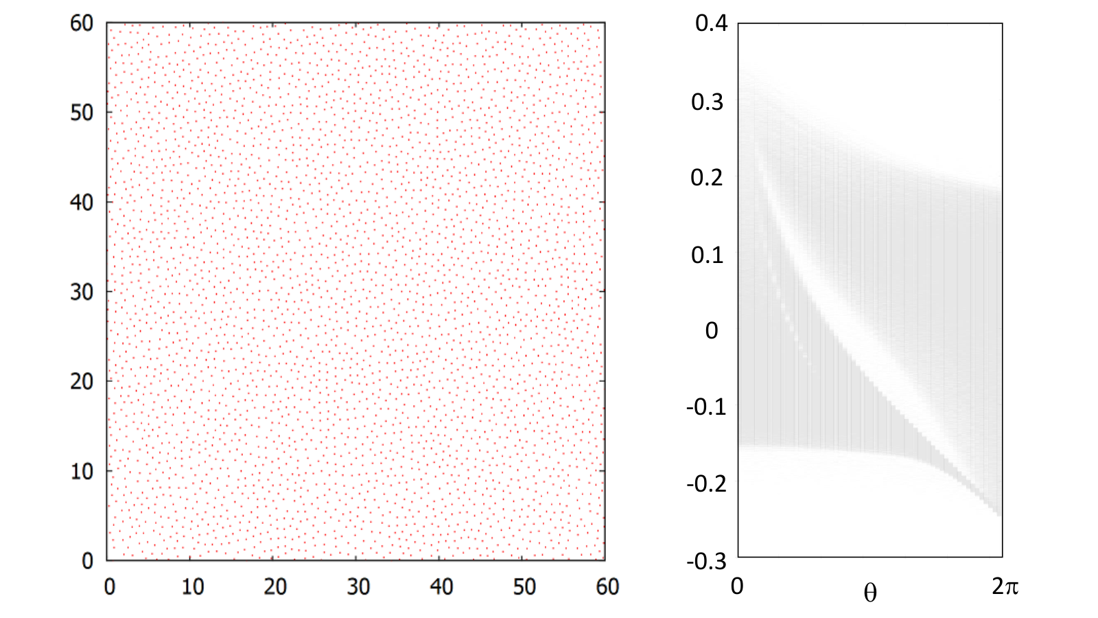
An example of a pattern generated with the above algorithm is shown in Fig. 2 for $L=60$. Note that the patterns are indeed periodic in the sense that, if the square $[0,L]\times[0,L]$ is wrapped in a torus, one will be unable to detect where the edges of the square were. For the same reason, we can periodically extend the pattern over the whole $\mathbb{R}^{2}$ without violating the constraints. We mentioned this detail because it relates to the program of finding periodic approximates of a pattern [6, 7]. In our context, the patterns we are interested in are actually defined by the thermodynamic limit of the periodic ones. More precisely, note that every time the algorithm is run for a fixed $L$, the pattern will be different from the previous. Hence we are dealing with a family of patterns which can be periodically extended over the whole space. Let $\Omega_{L}$ be the set of $L$-periodic patterns that we can generate with our algorithm, which we close in the standard topology of the space of Delone sets (see Proposition 4.4). The $\Omega_{L}$ spaces are invariant with respect to the translations of $\mathbb{R}^{2}$ and they form an inductive tower of compact topological spaces:

The “configuration” space of the infinite patterns is

which is a compact space, invariant to the translations $T$ of $\mathbb{R}^{2}$. The pair $(\Omega,\mathbb{R}^{2},T)$ is then a topological dynamical system, which also comes equipped with an invariant probability measure. Indeed, the finite volume algorithm determines entirely the probability of a $\mathcal{L}_{L}\in\Omega_{L}$ pattern to occur. Note that rigidly shifted patterns on the $L$-torus occur with equal probabilities. We denote by $\mathbf{P}_{L}$ the associated finite-volume probability measure, which is invariant to the cyclic shifts of the $L$-torus. Then the measure $\mathbf{P}$ on $\Omega$ can be defined as the unique measure whose traces over $\bar{\Omega}_{2^{n}L}$ coincide with $\mathbf{P}_{2^{n}L}$ for all $n=1,2,\ldots$, where

One important issue is whether the measure $\mathbf{P}$ is ergodic, which at this point we must assume.

The model Hamiltonian used in our simulations is:

Here, $e^{\imath\theta\,x\wedge x^{\prime}}$ is the usual Peierls phase factor [75] encoding the presence of a magnetic field, with $x\wedge x^{\prime}=\tfrac{1}{2}(x_{1}x^{\prime}_{2}-x_{2}x^{\prime}_{1})$ being the oriented area of the triangle made out of $x$, $x^{\prime}$ and the origin, and $\theta$ is the strength of the magnetic field in some adjusted units. Note that no cutoff was introduced on the hopping range.

We selected from the configuration space $\Omega$ an $L$-periodic pattern $\mathcal{L}$ and adapted the Hamiltonian (17) on the $L$-torus. To comply with the periodic boundary conditions, the values of the magnetic field were restricted to the discrete values $\theta_{n}=\frac{4\pi n}{L}$, $n=0,1,\ldots$. The energy spectrum of $H_{\mathcal{L}_{L}}$ as function of $\theta$ is reported in Fig. 2. It has been computed for a single pattern with $L=120$ and we have verified that there are no visible variations from one pattern to another. The spectrum displays a clear large gap and in fact a second smaller gap is also visible. Upon a more careful inspection, both gaps are filled with low density spectrum and so are in fact mobility gaps.

Next, we turn our attention to the Hall conductance (1). In [79, Ch. 5], a set of very general principles has been formulated for computing correlations of the type seen in (1). For disordered crystals, the finite-volume algorithms based on these principles have been shown to converge exponentially fast to the thermodynamic limit. Given the periodic approximates discusses in the previous section, the amorphous solid is covered as well by those principles, which we implemented here to evaluate Equation (1). For this, we:

• •

  Computed the Fermi projector $P_{F}^{(L)}=\chi_{(-\infty,E_{F}]}(H_{\mathcal{L}_{L}})$ using standard routines from functional analysis.

• •

  Made the commutators compatible with the periodic boundary conditions, by using the optimal substitution [77, 79]:

  $$\langle x|[P_{F},X_{j}]|y\rangle\rightarrow\left((x_{j}-y_{j})-L\left[\frac{2(x_{j}-y_{j})}{L}\right]\right)\,\langle x|P_{F}^{(L)}|y\rangle,$$

  (18)

  where on the right $x$ and $y$ represent the positions of the points inside $[0,L]\times[0,L]$ and the square brackets mean the integer part of a real number.

• •

  Evaluated the relevant matrix elements of the operator inside the trace in (1).

• •

  Computed the trace per volume using $\Tr_{\mathrm{Vol}}^{(L)}\{\cdot\}=\frac{1}{N}\Tr\{\cdot\}$.

A map of the Hall conductance as function of Fermi energy and magnetic strength, as computed with the above algorithm, is reported in Fig. 3 for three increasing system sizes $L=60$, 80 and 100. There we can observe a broad band where the Hall conductance takes the quantized value 1 and several narrower bands where the Hall conductance takes appreciable values. These bands become sharper as the simulation size is increased. The broad band and the first narrow band is consistent with the mobility gaps seen in Fig. 2, but notice that the broad band where $\sigma_{H}=1$ extends much further than the region of low spectral density visible with the eye in Fig. 2.

Fig. 4 shows the sections $\theta\simeq 1.5$ of the intensity maps from Fig. 3, together with the numerical values of $\sigma_{H}$ at $E_{F}=0.1$. As one can see, the quantization is extremely precise even for the smallest system size and for the largest system size the quantization holds with eight digits of precision. This is more remarkable given that $\sigma_{H}$ was computed from a single pattern configuration. This leaves very little doubt that, similar to disordered crystals, quantization principles are again at work for the amorphous solid; a fact which is confirmed in the following sections.

For the reader’s convenience, we collect in this section the minimal and quite standard background on point patterns needed for following sections. We take this opportunity to fix our notation. We start by fixing positive numbers $0<r<R<\infty$.

The space of Delone sets is obviously invariant to the $\mathbb{R}^{d}$ action $\mathcal{L}\mapsto\mathcal{L}+a$ for any $a\in\mathbb{R}^{d}$. These translations act as homeomorphisms in the topology of the space of Delone sets introduced above.

A groupoid is a small category where all morphisms are invertible. A more user-friendly characterisation of a groupoid is a set $\mathcal{G}$ with an inverse map, $\mathcal{G}\ni\gamma\mapsto\gamma^{-1}\in\mathcal{G}$, partially defined multiplication, $\mathcal{G}^{(2)}\ni(\gamma_{1},\gamma_{2})\mapsto\gamma_{1}\gamma_{2}\in\mathcal{G}$ for $\mathcal{G}^{(2)}\subset\mathcal{G}\times\mathcal{G}$, and space of units $\mathcal{G}^{(0)}$. We can define the source and range maps $r,s:\mathcal{G}\to\mathcal{G}^{(0)}$ as $s(\gamma)=\gamma^{-1}\gamma$ and $r(\gamma)=\gamma\gamma^{-1}$. In particular $(\gamma_{1},\gamma_{2})\in\mathcal{G}^{(2)}$ if and only if $s(\gamma_{1})=r(\gamma_{2})$. Topological structure can also be added if $\mathcal{G}$ is a locally compact Hausdorff space, where we require the multiplication and inverse maps to be continuous. A groupoid is called étale if $r$ is a local homeomorphism.

If the lattice $\widetilde{\mathcal{L}}$ is aperiodic, i.e. there is no $x\neq 0\in\mathbb{R}^{d}$ such that $\widetilde{\mathcal{L}}-x=\widetilde{\mathcal{L}}$, then $\mathcal{G}$ can also be described as the groupoid from the étale equivalence relation on $\Xi\times\Xi$,

Note that the topology on $R_{\Xi}$ is different than the subspace topology of $\Xi\times\Xi$. For lattices that are not aperiodic, the $C^{*}$-algebra of the groupoid coming from the orbit equivalence relation $R_{\Xi}$ will not be the correct algebra to model a physical system. See [54] for more on these issues.

Two groupoid elements $\gamma_{1}$ and $\gamma_{2}$ can be composed if $s(\gamma_{1})=r(\gamma_{2})$. Therefore for the case of the transversal groupoid, we can characterize the space of composable elements as

One uses this (partial) multiplication to construct a convolution algebra for the groupoid $\mathcal{G}$. Here, the groupoid algebra [53] will be twisted by a cocycle to account for the presence of a magnetic field. The interested reader may consult [87] for a comprehensive overview of the general groupoid $C^{*}$-construction including the twisted case.

As the name suggests, groupoid $2$-cocycles give rise to classes in the cohomolgy group $H^{2}(\mathcal{G},\mathbb{T})$, where if $\sigma$ is cohomologous to $\sigma^{\prime}$, then the corresponding (full or reduced) twisted groupoid $C^{*}$-algebras are isomorphic.

We encode a magnetic twist on our groupoid via a construction from [12], which considered twisted crossed products of commutative $C^{*}$-algebras. We construct a magnetic field in $d$ dimensions as a $2$-form $B\in\bigwedge^{2}\mathbb{R}^{d}$. Using coordinates $B$ can be seen as an anti-symmetric matrix $(B^{j,k})_{j,k=1}^{d}$ such that

We then define, for $x,\,y,\,z\in\mathcal{L}$, $\Gamma_{\mathcal{L}}\langle x,y,z\rangle=\int_{\langle x,y,z\rangle}B$ as the magnetic flux through the triangle $\langle x,y,z\rangle\subset\mathbb{R}^{d}\times\mathbb{R}^{d}$ with corners $x,\,y,\,z\in\mathcal{L}$. In most cases of interest, $B$ is a closed $2$-form, $B=\mathrm{d}A$, and so we can write the magnetic flux in the more familiar expression $\Gamma_{\mathcal{L}}\langle x,y,z\rangle=\int_{\langle x,y,z\rangle}\mathrm{d}A$. For this work, we will only consider systems with constant magnetic field strength and so the magnetic flux can be written using the anti-symmetric matrix $(B^{j,k})$ and coordinates of $x,y,z\in\mathcal{L}$.

With the preliminaries done, we define a magnetic twist via the 2-cocycle $\sigma:\mathcal{G}^{(2)}\to\mathbb{T}$,

as $((\mathcal{L},x),(\mathcal{L}-x,y))\in\mathcal{G}^{(2)}$ implies $0,\,x,\,x+y\in\mathcal{L}$. It is straightforward to see that for a $2$-dimensional lattice with magnetic field strength $\theta$, our twist coincides with Peierls phase factor in (17). The cocycle condition (20) on $\sigma$ translates into the condition that, for any $x$, $y$ and $z$ such that $x,\ x+y,\ x+y+z\in\mathcal{L}$,

which follows from Stokes’ Theorem and the observation that

We also note that our cocycle has the property that $\sigma((\mathcal{L},x),(\mathcal{L}-x,-x))=1$ for any $(\mathcal{L},x)\in\mathcal{G}$, which will simplify many of our formulas.

Given the groupoid $\mathcal{G}$ and cocycle $\sigma$, we can construct the twisted convolution $\ast$-algebra $C_{c}(\mathcal{G})$ where the elements are functions with compact support over $\mathcal{G}$ and the operations are,

The cocycle condition (20) on $\sigma$ ensures that $C_{c}(\mathcal{G})$ is associative and it is a simple check that $(f_{1}\ast f_{2})^{\ast}=f_{2}^{*}\ast f_{1}^{*}$. The algebra $C_{c}(\mathcal{G})$ is unital with the unit $1(\mathcal{L},x)=\delta_{x,0}$. Furthermore, it accepts a family of canonical representations, $\{\pi_{\mathcal{L}}\}_{\mathcal{L}\in\Xi}$, indexed by $\mathcal{L}\in\Xi$ and defined by the maps $\pi_{\mathcal{L}}:C_{c}(\mathcal{G})\to\mathcal{B}[\ell^{2}(\mathcal{L})]$,

One can check that $\pi_{\mathcal{L}}(f_{1}\ast f_{2})=\pi_{\mathcal{L}}(f_{1})\pi_{\mathcal{L}}(f_{2})$ and $\pi_{\mathcal{L}}(f^{*})=\pi_{\mathcal{L}}(f)^{*}$ so $\pi_{\mathcal{L}}$ is indeed a $\ast$-representation. Also, $\pi_{\mathcal{L}}(1)=1_{\mathcal{B}[\ell^{2}(\mathcal{L})]}$.

The next result gives a covariance for representations that come from lattices in the same orbit, which needs to be verified with care when the cocycle is present.

In this section we introduce a set of canonical derivations and invariant trace for $C^{*}_{r}(\mathcal{G},\sigma)$. Along the way, we introduce the smooth and Sobolev algebras which will play central roles.

References

- [1] A. Agarwala and V. B. Shenroy. Topological Insulators in Amorphous Systems. Phys. Rev. Lett. 118 (2017), 236402.
- [2] M. Aizenman and S. Molchanov. Localization at large disorder and at extreme energies: An elementary derivations. Comm. Math. Phys. 157 (1993), no. 2, 245–278.
- [3] S. Baaj and P. Julg. Théorie bivariante de Kasparov et opérateurs non bornés dans les -modules hilbertiens. C. R. Acad. Sci. Paris Sér. I Math 296 (1983), no. 21, 875–878.
- [4] F. Baboux, E. Levy, A. Lemaitre, C. Gómez, E. Galopin, L. L. Gratiet, I. Sagnes, A. Amo, J. Bloch and E. Akkermans. Measuring topological invariants from generalized edge states in polaritonic quasicrystals. Phys. Rev. B 95 (2017), 161114(R).
- [5] M. A. Bandres, M. C. Rechtsman and M. Segev. Topological photonic quasicrystals: Fractal topological spectrum and protected transport. Phys. Rev. X 6 (2016), 011016.
- [6] S. Beckus. Spectral approximation of aperiodic Schrödinger operators. PhD Thesis, Friedrich-Schiller-University, Jena, (2016).
- [7] S. Beckus, J. Bellissard and G. De Nittis. Spectral continuity for aperiodic quantum systems. arXiv:1709.00975 (2017).
- [8] J. Bellissard. K-theory of C∗-algebras in solid state physics. in T. Dorlas, M. Hugenholtz, M. Winnink, editors, Lecture Notes in Physics 257, pages 99–156, Springer-Verlag, Berlin, (1986).
- [9] J. Bellissard, A. van Elst and H. Schulz-Baldes. The non-commutative geometry of the quantum Hall-effect. J. Math. Phys. 35 (1994), 5373–5451.
- [10] J. Bellissard, R. Benedetti and J.-M. Gambaudo. Spaces of tilings, finite telescopic approximations and gap-labeling. Comm. Math. Phys. 261 (2006), no. 1, 1–41.
- [11] J. Bellissard, D. J. L. Herrmann and M. Zarrouati. Hulls of aperiodic solids and gap labelling theorems. Directions in Mathematical Quasicrystals. Volume 13 of CIRM Monograph Series (2000), 207–259.
- [12] F. Belmonte, M. Lein, and M. Măntoiu. Magnetic twisted actions on general abelian -algebras. J. Operator Theory 69 (2013), no. 1, 33–58.
- [13] M. Benameur, A. L. Carey, J. Phillips, A. Rennie, F. A. Sukochev, and K. P. Wojciechowski. An analytic approach to spectral flow in von Neumann algebras. In B. Booß-Bavnbek, S. Klimek, M. Lesch, and W. Zhang, editors, Analysis, Geometry and Topology of Elliptic Operators, pages 297–352. World Scientific Publishing (2006).
- [14] B. A. Bernevig, T. L. Hughes and S.-C. Zhang. Quantum spin Hall effect and topological phase transition in HgTe quantum wells, Science 314 (2006), 1757.
- [15] G. D. Birkhoff. Proof of the ergodic theorem, Proc. Natl. Acad. Sci. 17, 656-660 (1931).
- [16] D. D. Bleecker and B. Booß-Bavnbek. Index theory with applications to mathematics and physics. International Press, Boston, (2013).
- [17] C. Bourne. Topological states of matter and noncommutative geometry. PhD Thesis, Australian National University, (2015).
- [18] C. Bourne and A. Rennie. Chern numbers, localisation and the bulk-edge correspondence for continuous models of topological phases. arXiv:1611.06016 (2016).
- [19] C. Bourne and H. Schulz-Baldes. Application of semifinite index theory to weak topological phases. In D. R. Wood, J. De Gier, C. E. Praeger and T. Tao, editors, 2016 MATRIX Annals, pages 203–227, Springer International Publishing (2018). arXiv:1612.01613.
- [20] B. Bradlyn, L. Elcoro, J. Cano, M. G. Vergniory, Z. Wang, C. Felser, M. I. Aroyo, B. A. Bernevig. Topological quantum chemistry. Nature 547 (2017), 298–305.
- [21] A. P. Calderón. The analytic calculation of the index of elliptic equations. Proc. National Academy of Sciences USA 57 (1967), 1193–1196.
- [22] A. L. Carey, V. Gayral, A. Rennie and F. A. Sukochev. Index theory for locally compact noncommutative geometries. Mem. Amer. Math. Soc. 231 (2014), no. 2.
- [23] A. L. Carey, K. C. Hannabuss, V. Mathai and P. McCann. Quantum Hall Effect on the hyperbolic plane. Comm. Math. Phys. 190 (1998), 629–673.
- [24] A. L. Carey, K. C. Hannabuss and V. Mathai. Quantum Hall Effect on the hyperbolic plane in the presence of disorder. Lett. Math. Phys. 47 (1999), 215–236.
- [25] A. L. Carey, J. Phillips and A. Rennie. Spectral triples: examples and index theory. In Noncommutative geometry and physics: renormalisation, motives, index theory, pages 175–265, Eur. Math. Soc., Zürich (2011).
- [26] A. L. Carey, J. Phillips, A. Rennie and F. A. Sukochev. The Hochschild class of the Chern character for semifinite spectral triples. J. Funct. Anal. 213 (2004), no. 1, 111–153.
- [27] A. L. Carey, J. Phillips, A. Rennie and F. A. Sukochev. The local index formula in semifinite von Neumann algebras I: Spectral flow. Adv. Math. 202 (2006), no. 2, 451–516.
- [28] A. L. Carey, J. Phillips, A. Rennie and F. A. Sukochev. The local index formula in semifinite von Neumann algebras II: The even case. Adv. Math. 202 (2006), no. 2, 517–554.
- [29] A. Connes. Noncommutative Geometry. Academic Press, San Diego, (1994).
- [30] A. Connes and H. Moscovici. The local index formula in noncommutative geometry. Geom. Funct. Anal. 5 (1995), 174–243.
- [31] G. Cortiñas. Algebraic v. Topological K-Theory: A Friendly Match. in G. Cortiñas, editor, Topics in Algebraic and Topological K-Theory, pages 103–165, Springer, Berlin, (2011).
- [32] A. Dareau, E. Levy, M. B. Aguilera, R. Bouganne, E. Akkermans, F. Gerbier and J. Beugnon. Direct measurement of Chern numbers in the diffraction pattern of a Fibonacci chain. arXiv:1607.00901v1 (2016).
- [33] K. Davidson. -algebras by example. American Mathematical Society, Providence, (1996).
- [34] G. De Nittis and M. Lein. On the role of symmetries in the theory of photonic crystals. Annals of Physics 350 (2014), 568–587.
- [35] G. De Nittis and M. Lein. The Schrödinger formalism of electromagnetism and other classical waves: how to make quantum-wave analogies rigorous. arXiv:1710.10148 (2017).
- [36] R. L. Dobrushin, Y. G. Sinai, Y. M. Sukhov. Dynamical systems of statistical mechanics and kinetic equations. In Y. G. Sinai, editor, Dynamical Systems II, Springer, Berlin, (1989).
- [37] T. Fack, H. Kosaki. Generalised -numbers of -measurable operators. Pac. J. Math. 123 (1986), no. 2, 269–300.
- [38] B. V. Fedosov. Analytic formulas for the index of elliptic operators. Trans. Mosc. Math. Soc. 30 (1974), 159–240.
- [39] L. Fu and C. L. Kane. Topological insulators in three dimensions. Phys. Rev. B 76 (2007), 045302.
- [40] J. N. Fuchs and J. Vidal. Hofstadter butterfly of a quasicrystal. Phys. Rev. B 94 (2016), 205437.
- [41] F. Germinet, P. Müller and C. Rojas-Molina. Ergodicity and dynamical localization for Delone-Anderson operators. Rev. Math Phys. 27 (2015), no. 9, 1550020.
- [42] J. M. Gracia-Bondía, J. C. Várilly and H. Figueroa. Elements of Noncommutative Geometry. Birkhäuser Advanced Texts Basler Lehrbücher. Birkhäuser, Boston, (2001).
- [43] J. Großmann and H. Schulz-Baldes. Index pairings in presence of symmetries with applications to topological insulators. Comm. Math. Phys., 343 (2016), no. 2, 477–513.
- [44] M. Hafezi, S. Mittal, J. Fan, A. Migdall and J. M. Taylor. Imaging topological edge states in silicon photonics. Nature Photonics 7 (2013), 1001–1005.
- [45] F. D. M. Haldane. Model for a quantum Hall-effect without Landau levels: Condensed-matter realization of the parity anomaly. Phys. Rev. Lett. 61 (1988), 2015–2019.
- [46] M. Herman, E. Prodan and Y. Shmalo. The K-theoretic bulk-boundary principle for dynamically patterned resonators. In preparation.
- [47] N. Higson and J. Roe. Analytic K-Homology. Oxford Univ. Press, Oxford, (2000).
- [48] D. Hsieh, D. Qian, L. Wray, Y. Xia, Y. S. Hor, R. J. Cava and M. Z. Hasan. A topological Dirac insulator in a quantum spin Hall phase. Nature 452 (2008), 970–974.
- [49] W. Hu, J. C. Pillay, K. Wu, M. Pasek, P. P. Shum and Y. D. Chong. Measurement of a topological edge invariant in a microwave network. Phys. Rev. X 5 (2015), 011012.
- [50] C. L. Kane and T. Lubensky. Topological boundary modes in isostatic lattices. Nature Physics 10, 39-45 (2013).
- [51] C. L. Kane and E. J. Mele. Quantum spin Hall effect in graphene. Phys. Rev. Lett. 95 (2005), 226801.
- [52] C. L. Kane and E. J. Mele. topological order and the quantum spin Hall effect. Phys. Rev. Lett. 95 (2005), 146802.
- [53] J. Kellendonk Noncommutative geometry of tilings and gap labelling. Rev. Math. Phys. 7 (1995), 1133–1180.
- [54] J. Kellendonk. The local structure of tilings and their integer group of coinvariants. Comm. Math. Phys. 187 (1997), 115–157.
- [55] A. Kitaev. Anyons in an exactly solved model and beyond. Annals of Physics 321 (2006), 2–111.
- [56] A. Kitaev. Periodic table for topological insulators and superconductors. In Vladimir Lebedev and Mikhail Feigel’man, editors, Adv. Theor. Phys.: Landau Memorial Conference, volume 1134, pages 22–30, AIP, (2009).
- [57] M. Koenig, S. Wiedmann, C. Bruene, A. Roth, H. Buhmann, L. W. Molenkamp, X.-L. Qi and S.-C. Zhang. Quantum spin Hall insulator state in HgTe quantum wells. Science 318 (2007), 766-770.
- [58] Y. E. Kraus, Y. Lahini, Z. Ringel, M. Verbin and O. Zilberberg. Topological states and adiabatic pumping in quasicrystals. Phys. Rev. Lett. 109 (2012), 106402.
- [59] Y. E. Kraus, Z. Ringel and O. Zilberberg. Four-dimensional quantum Hall effect in a two-dimensional quasicrystal. Phys. Rev. Lett. 111 (2013), 226401.
- [60] Y. E. Kraus and O. Zilberberg. Topological equivalence between the Fibonacci quasicrystal and the Harper model. Phys. Rev. Lett. 109 (2012), 116404.
- [61] J. Kruthoff, J. de Boer, J. van Wezel, C. L. Kane and R.-J. Slager. Topological classification of crystalline insulators through band structure combinatorics. Phys. Rev. X, 7 (2017), 041069.
- [62] Y. Kubota. Controlled topological phases and bulk-edge correspondence. Comm. Math. Phys. 349 (2017), no. 2, 493–525.
- [63] T. Kühne and E. Prodan. Disordered crystals from first principles I: quantifying the configuration space. Annals of Physics, 391 (2018), 120–149.
- [64] D. Lenz, N. Peyerimhoff and I. Veselić. Groupoids, von Neumann algebras and the integrated density of states. Math. Phys. Anal. Geom. 10 (2007), no. 1, 1–41.
- [65] E. Levy, A. Barak, A. Fisher and E. Akkermans. Topological properties of Fibonacci quasicrystals : A scattering analysis of Chern numbers. arXiv:1509.04028v3 (2015).
- [66] T. A. Loring and M. B. Hastings. Disordered topological insulators via -algebras. Europhysics Lett. 92 (2011), 67004.
- [67] T. A. Loring and H. Schulz-Baldes. Finite volume calculation of K-theory invariants. New York J. Math. 22 (2017), 1111–1140.
- [68] T. A. Loring and H. Schulz-Baldes. The spectral localizer for even index pairings. arXiv:1802.04517 (2018).
- [69] B. Mesland. Groupoid cocycles and -theory. Münster J. of Math. 4 (2011), 227–250.
- [70] N. P. Mitchell, L. M. Nash, D. Hexner, A. Turner and W. T. M. Irvine. Amorphous topological insulators constructed from random point sets. Nature Physics, 14 (2018), 380–385.
- [71] J. E. Moore and L. Balents. Topological invariants of time-reversal-invariant band structures. Phys. Rev. B 75 (2007), 121306.
- [72] P. Muhly, J. Renault and D. P. Williams. Equivalence and isomorphism for groupoid -algebras. J. Operator Theory 17 (1987), 3–22.
- [73] L. M. Nash, D. Kleckner, A. Read, V. Vitelli, A. M. Turner and W. T. M. Irvine. Topological mechanics of gyroscopic metamaterials. Proc. Nat. Acad. Sci. 112 (2015), 14495-14500.
- [74] D. Pask, A. Rennie and A. Sims. The noncommutative geometry of -graph -algebras. J. -Theory 1 (2008), 259–304.
- [75] R. E. Peierls. Zur Theorie des Diamagnetismus von Leitungselektronen. Zeitschrift für Phys. 80 (1933), 763–791.
- [76] H. C. Po, A. Vishwanath and Haruki Watanabe. Symmetry-based indicators of band topology in the 230 space groups. Nat. Commun. 8 (2017), 50.
- [77] E. Prodan. Quantum transport in disordered systems under magnetic fields: A study based on operator algebras. Appl. Math. Res. Express 2013 (2013), 176–255.
- [78] E. Prodan. Virtual topological insulators with real quantized physics. Phys. Rev. B 91 (2015), 245104.
- [79] E. Prodan. A Computational non-commutative geometry program for topological insulators. Springer, Berlin, (2017).
- [80] E. Prodan and C. Prodan. Topological phonon modes and their role in dynamic instability of microtubules. Phys. Rev. Lett. 103 (2009), 248101.
- [81] E. Prodan, B. Leung and J. Bellissard. The non-commutative n-th Chern number (). J. Phys. A: Math. Theor. 46 (2013), 485202.
- [82] E. Prodan and H. Schulz-Baldes. Non-commutative odd Chern numbers and topological phases of disordered chiral systems. J. Func. Anal. 271 (2016), 1150–1176.
- [83] E. Prodan and H. Schulz-Baldes. Bulk and Boundary Invariants for Complex Topological Insulators: From -Theory to Physics. Springer Int. Pub., Switzerland (2016).
- [84] E. Prodan and J. Bellissard. Mapping the current-current correlation function near a quantum critical point. Ann. Phys. 368 (2016), 1–15.
- [85] J. Paulose, B.-G. Chen and V. Vitelli. Topological modes bound to dislocations in mechanical metamaterials. Nature Physics 11 (2015), 153-156.
- [86] M. C. Rechtsman, J. M. Zeuner, Y. Plotnik, Y. Lumer, D. Podolsky, F. Dreisow, S. Nolte, M. Segev and A. Szameit. Photonic floquet topological insulators. Nature 496 (2013), 196–200.
- [87] J. Renault. A groupoid approach to -algebras. Lecture Notes in Mathematics, vol. 793, Springer-Verlag (1980).
- [88] A. Rennie. Smoothness and locality for nonunital spectral triples. -Theory 28 (2003), 127–165.
- [89] C. Rojas-Molina. Random Schrödinger Operators on discrete structures. arXiv:1710.02293 (2017).
- [90] D. Ruelle. Statistical Mechanics: Rigorous Results. W. A. Benjamin, London, (1969).
- [91] S. Ryu, A. P. Schnyder, A. Furusaki and A. W. W. Ludwig. Topological insulators and superconductors: tenfold way and dimensional hierarchy. New J. Phys. 12, 065010 (2010).
- [92] L. Sadun. Topology of Tiling Spaces. American Mathematical Society, Providence, (2008).
- [93] L. Sadun and R. W. Williams. Tiling spaces are Cantor set fiber bundles. Ergodic Theory Dynam. Systems, 23 (2003), no. 1, 307–316.
- [94] J. Savinien. Cohomology and -theory of aperiodic tilings. PhD thesis, Georgia Institute of Technology (2008).
- [95] J. Savinien and J. Bellissard. A spectral sequence for the -theory of tiling spaces. Ergodic Theory Dynam. Systems 29 (2009), no. 3, 997–1031.
- [96] A. P. Schnyder, S. Ryu, A. Furusaki and A. W. W. Ludwig. Classification of topological insulators and superconductors in three spatial dimensions. Phys. Rev. B 78 (2008), 195125.
- [97] H. Schulz-Baldes and J. Bellissard. A kinetic theory for quantum transport in aperiodic media. J. Stat. Phys. 91 (1998), 991–1026.
- [98] H. Schulz-Baldes and J. Bellissard. Anomalous transport: a mathematical framework. Rev. Math. Phys. 10 (1998), 1–46.
- [99] K. Shiozaki, M. Sato and K. Gomi. Topological Crystalline Materials - General Formulation, Module Structure, and Wallpaper Groups. Phys. Rev. B 95 (2017), 235425.
- [100] K. Shiozaki, M. Sato and K. Gomi. Atiyah–Hirzebruch spectral sequence in band topology: general formalism and topological invariants for 230 space groups. arXiv:1802.06694 (2018).
- [101] A. Sims and D. P. Williams, Renault equivalence Theorem for reduced groupoid -algebras. J. Operator Theory 68 (2012), no. 1, 223–239.
- [102] J. C. W. Song and M. S. Rudner. Chiral plasmons without magnetic field. Proc. Nat. Acad. Sci. (PNAS) 113 (2016), 4658–4663.
- [103] D. Tanese, E. Gurevich, F. Baboux, T. Jacqmin, A. Lemaitre, E. Galopin, I. Sagnes, A. Amo, J. Bloch and E. Akkermans. Fractal Energy Spectrum of a Polariton Gas in a Fibonacci Quasiperiodic Potential. Phys. Rev. Lett. 112 (2014), 146404.
- [104] D.-T. Tran, A. Dauphin, N. Goldman and P. Gaspard. Topological Hofstadter insulators in a two-dimensional quasicrystal. Phys. Rev. B 91 (2015), 085125.
- [105] D. J. Thouless, M. Kohmoto, M. P. Nightingale and M. den Nijs. Quantized Hall conductance in a two-dimensional periodic potential Phys. Rev. Lett. 49 (1982), 405–408.
- [106] M. Verbin, O. Zilberberg, Y. E. Kraus, Y. Lahini and Y. Silberberg. Observation of topological phase transitions in photonic quasicrystals. Phys. Rev. Lett. 110 (2013), 076403.
- [107] M. Verbin, O. Zilberberg, Y. Lahini, Y. E. Kraus and Y. Silberberg. Topological pumping over a photonic Fibonacci quasicrystal. Phys. Rev. B 91 (2015), 064201.
- [108] Z. Wang, Y. Chong, J. D. Joannopoulos and M. Soljacic. Observation of unidirectional backscattering-immune topological electromagnetic states. Nature 461 (2009), 772–775.