Error estimates on ergodic properties of discretized Feynman–Kac semigroups

Grégoire Ferré Gabriel Stoltz Affiliation: Université Paris-Est, CERMICS (ENPC), Inria, F-77455 Marne-la-Vallée, France

August 24, 2026

Abstract

We consider the numerical analysis of the time discretization of Feynman–Kac semigroups associated with diffusion processes. These semigroups naturally appear in several fields, such as large deviation theory, Diffusion Monte Carlo or non-linear filtering. We present error estimates à la Talay–Tubaro on their invariant measures when the underlying continuous stochastic differential equation is discretized; as well as on the leading eigenvalue of the generator of the dynamics, which corresponds to the rate of creation of probability. This provides criteria to construct efficient integration schemes of Feynman–Kac dynamics, as well as a mathematical justification of numerical results already observed in the Diffusion Monte Carlo community. Our analysis is illustrated by numerical simulations.

1 Introduction

The study of Feynman–Kac semigroups for stochastic differential equations (SDEs) has been a topic of growing importance in the past two decades, since these dynamics are related to several theoretical and applied areas of mathematics. They can be seen as standard SDEs whose paths are reweighted according to the exponential of the time integral of some weight function.

Feynman–Kac semigroups naturally appear in large deviation theory, where they can be used to enhance the likelihood of observing rare fluctuations and henceforth computing cumulant generating functions [71, 15]. They also have important practical applications, such as in the Diffusion Monte Carlo (DMC) method [28], which is a probabilistic way of estimating the ground state energy of Schrödinger operators; or in computational statistics, in particular in (non-linear) filtering [10, 19], where relevant trajectories are selected from observations.

We focus in this paper on the bias arising from the time discretization of the underlying continuous stochastic dynamics and of the time integrated weight. Our interest resides in the ergodic properties of the discretization, namely the invariant measure as well as the average rate of creation of probability. Let us briefly present our setting and results. We study a system $q_{t}\in\mathcal{D}$ evolving in a $d$ -dimensional space, assumed to be compact (the extension to unbounded spaces poses non-trivial issues, as discussed at various places later on). Typically, $\mathcal{D}=\mathbb{T}^{d}$ (with $\mathbb{T}=\mathbb{R}\backslash\mathbb{Z}$ ) is a $d$ -dimensional torus. For convenience, we consider that the evolution is dictated by a stochastic differential equation with additive noise:

dq_{t}=b(q_{t})\,dt+\sigma\,dB_{t},

(1)

where $b:\mathcal{D}\to\mathbb{R}^{d}$ is a $\mathcal{C}^{\infty}(\mathcal{D})$ vector field, $\sigma>0$ and $B_{t}$ is a standard $d$ -dimensional Brownian motion. Note that the dynamics (1) may be non-reversible. Our results can be extended to dynamics with multiplicative noise upon appropriate modifications. The infinitesimal generator of the dynamics (1), defined on the core $\mathcal{S}=\mathcal{C}^{\infty}(\mathcal{D})$ , reads

\mathcal{L}=b\cdot\nabla+\frac{\sigma^{2}}{2}\Delta,

(2)

and we denote by $\mathcal{L}^{\dagger}$ the adjoint of $\mathcal{L}$ on $L^{2}(\mathcal{D})$ endowed with the Lebesgue measure. Since $\mathcal{D}$ is compact and $b$ is smooth, (1) admits a unique invariant distribution, denoted by $\nu$ , which is solution to the Fokker–Planck equation

\mathcal{L}^{\dagger}\nu=0,

see e.g. [59, 39, 46]. Denoting by $\mathcal{P}(\mathcal{D})$ the set of probability measures over $\mathcal{D}$ , Feynman–Kac type semigroups associated with a given weight function $W:\mathcal{D}\to\mathbb{R}$ evolve an initial probability measure $\mu\in\mathcal{P}(\mathcal{D})$ as follows: for any test function $\varphi\in\mathcal{S}$ ,

\Phi_{t}^{W}(\mu)(\varphi)=\frac{\mathbb{E}_{\mu}\left[\varphi(q_{t})\,\mathrm{e}^{\int_{0}^{t}W(q_{s})\,ds}\right]}{\displaystyle\mathbb{E}_{\mu}\left[\mathrm{e}^{\int_{0}^{t}W(q_{s})\,ds}\right]},

(3)

where the expectations run over initial conditions $q_{0}$ distributed according to $\mu$ and all realizations of (1). The family of mappings $\{\Phi_{t}^{W}\}_{t\geqslant 0}$ is a measure-valued non-linear semigroup in the sense that $\Phi_{t}^{W}:\mathcal{P}(\mathcal{D})\to\mathcal{P}(\mathcal{D})$ depends non-linearly on the initial condition and, for all $\mu\in\mathcal{P}(\mathcal{D})$ and $t,s\in\mathbb{R}_{+}$ , $\Phi_{t}^{W}(\Phi_{s}^{W}(\mu))=\Phi_{t+s}^{W}(\mu)$ . Such semigroups have been studied for a long time in the context of Diffusion Monte Carlo (DMC) [31, 4, 7, 70, 28] in order to estimate the principal eigenvalue of Schrödinger type operators $-\Delta+W$ , which correspond in our case to $b\equiv 0$ . They also appear in the large deviation community [30, 44, 65, 68, 55, 56] where they are related to the principal eigenvalue of $\mathcal{L}+W$ , which is the dual of the rate function – a result known as the Donsker-Varadhan formula [18, 71, 15, 68, 14]. Other fields such as non-linear filtering, Hidden Markov Models [38, 19, 20] and free energy computation [37, 36, 62, 47] also motivate the study of such semigroups.

As discussed in Section 2.1, the semigroup (3) converges in general to the average of $\varphi$ with respect to a tilted measure $\nu_{W}$ . More precisely, the operator $\mathcal{L}^{\dagger}+W$ has a largest eigenvalue $\lambda$ which is isolated from the remainder of the spectrum and non-degenerate, with associated eigenfunction $\nu_{W}$ , and

\Phi_{t}^{W}(\mu)(\varphi)\xrightarrow[t\to\infty]{}\,\int_{\mathcal{D}}\varphi\,d\nu_{W}

exponentially fast. We address in this work the time discretization of the semigroup (3) using a finite timestep $\Delta t$ . The underlying continuous evolution (1) is discretized by a Markov chain $(q^{n})_{n\in\mathbb{N}}$ and (3) is approximated as (using a simple quadrature rule for the time integral)

\Phi_{\Delta t,n}^{W}(\mu)(\varphi)=\frac{\displaystyle\mathbb{E}_{\mu}\left[\varphi(q^{n})\,\mathrm{e}^{\Delta t\sum_{i=0}^{n-1}W(q^{i})}\right]}{\displaystyle\mathbb{E}_{\mu}\left[\mathrm{e}^{\Delta t\sum_{i=0}^{n-1}W(q^{i})}\right]}.

(4)

Under mild assumptions on the discretization scheme (made precise in Section 2.2), the discrete semigroup (4) converges to an invariant measure $\nu_{W,\Delta t}$ in the following sense: for any test function $\varphi\in\mathcal{S}$ ,

\Phi_{\Delta t,n}^{W}(\mu)(\varphi)\xrightarrow[n\to+\infty]{}\,\int_{\mathcal{D}}\varphi\,d\nu_{W,\Delta t}.

The core of our work consists in making precise the difference between $\nu_{W}$ and $\nu_{W,\Delta t}$ . We aim in particular at designing numerical schemes leading to the smallest possible biases. Although a series of papers study the statistical error of estimators such as (4) (see [11, 13, 10, 60, 61]), there are, to our knowledge, no available estimates on the bias of the limiting measure with respect to $\Delta t$ . However, in the context of DMC (where we recall $b=0$ ), it was numerically observed that some discretizations provide first, second or fourth order of convergence in $\Delta t$ for the largest eigenvalue $\lambda$ of $\mathcal{L}+W$ , see for example [4, 70, 52, 63], and [23] for the numerical analysis in a simple case. The results presented in this paper provide a mathematical justification of such convergences, while extending them to the case $b\neq 0$ . Let us also mention that Hairer and Weare have studied in [34, 35] the convergence with respect to the timestep of discretized dynamics similar to the one we consider, over a finite time and for a finite population of replicas. They obtain in the limit $\Delta t\to 0$ a limiting process, the so-called Brownian fan.

We rely on the techniques developped since the works of Talay and Tubaro [67, 66], taking advantage of the analytical tools developed in a series of papers [51, 9, 1, 2, 6, 45, 46], in order to provide a systematic framework to study the bias in the timestep. More precisely, we show in Theorem 2 that there exist an integer $p\geqslant 1$ and a function $f$ solution to a Poisson equation (both depending on the numerical scheme at hand and the quadrature rule for the integral), such that, for all $\varphi\in\mathcal{S}$ ,

\int_{\mathcal{D}}\varphi\,d\nu_{W,\Delta t}=\int_{\mathcal{D}}\varphi\,d\nu_{W}+\Delta t^{p}\int_{\mathcal{D}}\varphi f\,d\nu_{W}+\mathrm{O}(\Delta t^{p+1}).

(5)

This result is very similar to those of weak backward error analysis on invariant probability measures of ergodic processes, see for example [9, 6, 45]. Moreover, as the computation of the principal eigenvalue $\lambda$ of the operator $\mathcal{L}+W$ is one of the main concerns in Feynman–Kac techniques, we provide in Theorem 3 the following error estimate:

\lambda_{\Delta t}:=\frac{1}{\Delta t}\log\left[\int_{\mathcal{D}}Q_{\Delta t}^{W}\mathds{1}\,d\nu_{W,\Delta t}\right]=\lambda+C\Delta t^{p}+\mathrm{O}(\Delta t^{p+1}),

(6)

where $Q_{\Delta t}^{W}$ is the evolution operator of the discretized dynamics with weight function $W$ . This result is interesting since it allows to justify the use of population dynamics methods for discretizations of diffusion processes, see [30, 65, 55] for rare events simulations, and [28] for DMC. Let us mention that, while the proof of (5) relies on previous works concerning error estimates on the invariant measure [67, 66, 6, 9, 45], the novelty of this work lies in taking into account the non-probability conserving feature of the dynamics. With this point of view and, odd as it may seem, formula (5) appears as a consequence of (6), and not conversely. An interpretation of this fact is that, in order to prove an error estimate on the invariant probability measure of this non probability-conserving dynamics, we must first show that the discretized process creates or destroys probability at a rate correct up to terms small in $\Delta t$ .

The paper is organized as follows. Section 2 is devoted to general properties of Feynman–Kac semigroups and their discretizations. We then present in Section 3 our main results concerning the numerical analysis of the error on the invariant probability measure, depending on the choice of the discretization scheme, before providing numerical applications in Section 4. Finally, Section 5 proposes possible extensions to this work. The proofs of the most technical results are gathered in Section 6.

2 Convergence properties of Feynman–Kac semigroups

We present in this section the setting of our study. In particular, we remind convergence results and some useful properties of continuous Feynman–Kac semigroups in Section 2.1, as well as convergence results for their discretizations in Section 2.2. Although these results are known, we believe that it is useful to gather them here to allow for a self-contained presentation of the numerical analysis framework developped in Section 3.

2.1 Continuous dynamics

We denote by $P_{t}$ the evolution operator associated with the process $(q_{t})_{t\geqslant 0}$ in (1): for all $\mu\in\mathcal{P}(\mathcal{D})$ and $\varphi\in\mathcal{S}$ ,

P_{t}(\mu)(\varphi)=\mathbb{E}_{\mu}\left[\varphi(q_{t})\right].

Its weighted counterpart is

P_{t}^{W}(\mu)(\varphi)=\mathbb{E}_{\mu}\left[\varphi(q_{t})\,\mathrm{e}^{\int_{0}^{t}W(q_{s})\,ds}\right].

The infinitesimal generators of $P_{t}$ and $P_{t}^{W}$ are respectively $\mathcal{L}$ and $\mathcal{L}+W$ , where we denote with some abuse of notation by $W$ the multiplication operator by the function $W$ . Whether a statement corresponds to the function $W$ or the associated multiplication operator should be clear from the context. We assume in the sequel that the function $W$ is smooth, so that the associated multiplication operator stabilizes the core $\mathcal{S}$ .

The existence of a spectral gap for the generator $\mathcal{L}+W$ and its adjoint is a key ingredient for our study. Here and in the sequel, and otherwise explicitly mentioned, all operators are considered on the Hilbert space

L^{2}(\nu)=\left\{\varphi\textrm{ measurable}\,\left|\,\int_{\mathcal{D}}|\varphi|^{2}d\nu<+\infty\right.\right\}.

For a given closed operator $T$ on $L^{2}(\nu)$ , we denote by $T^{*}$ the adjoint of $T$ in $L^{2}(\nu)$ . In particular,

\forall\,(\varphi,\psi)\in\mathcal{S}^{2},\qquad\int_{\mathcal{D}}(T\varphi)\psi\,d\nu=\int_{\mathcal{D}}\varphi\left(T^{*}\psi\right)\,d\nu.

In this functional framework, the reversibility of the dynamics is equivalent to the self-adjointness of $\mathcal{L}$ on $L^{2}(\nu)$ . We however do not assume that this is the case, and this is why we need to distinguish between eigenelements of $\mathcal{L}$ and $\mathcal{L}^{*}$ . We can then state the following.

Proposition 1.

The operator $\mathcal{L}+W$ , considered on $L^{2}(\nu)$ , has a real isolated principal eigenvalue $\lambda$ with associated eigenfunction $\hat{h}_{W}\in\mathcal{S}$ normalized as

(\mathcal{L}+W)\hat{h}_{W}=\lambda\,\hat{h}_{W},\qquad\int_{\mathcal{D}}\hat{h}_{W}\,d\nu=1.

(7)

The operator $\mathcal{L}^{*}+W$ then also admits $\lambda$ as a real isolated principal eigenvalue, with associated eigenfunction $h_{W}\in\mathcal{S}$ normalized as

(\mathcal{L}^{*}+W)h_{W}=\lambda\,h_{W},\qquad\int_{\mathcal{D}}h_{W}\,d\nu=1.

(8)

Moreover, the functions $\hat{h}_{W}$ and $h_{W}$ are positive.

The fact that $\hat{h}_{W},h_{W}\in\mathcal{S}$ is a consequence of elliptic regularity. Let us emphasize that, as a consequence of (8), the measure

\nu_{W}=h_{W}\,\nu

is the only invariant probability measure for the evolution encoded by $P_{t}^{W-\lambda}$ . Moreover, when the underlying diffusion is reversible, i.e. $b=-\nabla V$ and $\nu(dq)=Z^{-1}\,\mathrm{e}^{-2V(q)/\sigma^{2}}\,dq$ , the operator $\mathcal{L}$ is self-adjoint ( $\mathcal{L}^{*}=\mathcal{L}$ ) so that $\hat{h}_{W}=h_{W}$ . When $W=0$ , it simply holds $h_{W}=\mathds{1}$ whatever $b$ .

Proof.

It is shown in [29] that the operator $\mathcal{L}+W$ has a real isolated principal eigenvalue when considered as an operator on $C^{0}(\mathcal{D})$ , the space of continuous functions over $\mathcal{D}$ . This can be proved using the Krein–Rutman theorem [22]. On the other hand, standard results of spectral theory of elliptic operators on bounded domains show that $\mathcal{L}+W$ on $L^{2}(\nu)$ has a discrete spectrum, which is bounded above [58]. The first eigenvalue cannot be degenerate since the associated eigenvectors are smooth by elliptic regularity and are therefore also eigenvectors of $\mathcal{L}+W$ considered as an operator on $C^{0}(\mathcal{D})$ . Finally, the positivity of $\hat{h}_{W}$ and $h_{W}$ follows from the fact that the evolution semigroup $P_{t}^{W}$ and its adjoint are operators with smooth and positive transition kernels (since the noise is non-degenerate), together with the equalities $P_{t}^{W}\hat{h}_{W}=\mathrm{e}^{\lambda t}\hat{h}_{W}$ and $(P_{t}^{W})^{*}h_{W}=\mathrm{e}^{\lambda t}h_{W}$ . ∎

In what follows, we use the subspaces $L_{W}^{2}(\nu)$ and $\mathcal{S}_{W}$ of functions of average $0$ with respect to $\nu_{W}$ :

L_{W}^{2}(\nu)=\left\{\varphi\in L^{2}(\nu)\ \middle|\ \int_{\mathcal{D}}\varphi\,d\nu_{W}=0\right\},\qquad\mathcal{S}_{W}=\left\{\varphi\in\mathcal{S}\ \middle|\ \int_{\mathcal{D}}\varphi\,d\nu_{W}=0\right\}.

We also introduce the measure $\hat{\nu}_{W}=\hat{h}_{W}\,\nu$ , the space

\hat{\mathcal{S}}_{W}=\left\{\varphi\in\mathcal{S}\ \middle|\ \int_{\mathcal{D}}\varphi\,d\hat{\nu}_{W}=0\right\},

and we denote by

\delta_{W}=\inf\Big\{\lambda-\mathrm{Re}(z),\,z\in\sigma(\mathcal{L}+W)\setminus\{\lambda\}\Big\}>0

(9)

the spectral gap of $\mathcal{L}+W$ in $L^{2}(\nu)$ . The fact that the largest eigenvalue $\lambda$ is a priori non-zero corresponds to a possible creation ( $\lambda>0$ ) or destruction ( $\lambda<0$ ) of probability induced by the source term $W$ , which plays the role of an importance sampling function. The statement about the spectral gap in Proposition 1 implies the convergence of the Feynman–Kac semigroup (3), as stated in the following result.

Proposition 2.

There exists $C>0$ such that, for all $\mu\in\mathcal{P}(\mathcal{D})$ and $\varphi\in L^{2}(\nu)$ ,

\forall\,t\geqslant 1,\qquad\left|\Phi_{t}^{W}(\mu)(\varphi)-\int_{\mathcal{D}}\varphi\,d\nu_{W}\right|\leqslant C\left\|\varphi\right\|_{L^{2}(\nu)}\mathrm{e}^{-\delta_{W}t},

(10)

where $\delta_{W}$ is defined in (9).

As made clear in the proof of this result (see Section 6.1), it is possible to consider any observable $\varphi\in L^{2}(\nu)$ even if $\mu$ is singular. This is due to the regularizing properties of the underlying diffusion for positive times, and explains why the convergence result is stated only for times $t\geqslant 1$ . The next proposition will be frequently used in this work.

Proposition 3.

It holds

\int_{\mathcal{D}}W\,d\nu_{W}=\lambda.

(11)

Proof.

Integrating both sides of (8) on $\mathcal{D}$ ,

\int_{\mathcal{D}}W\,d\nu_{W}=\int_{\mathcal{D}}\lambda h_{W}\,d\nu-\int_{\mathcal{D}}\mathcal{L}^{*}h_{W}\,d\nu=\lambda\int_{\mathcal{D}}h_{W}\,d\nu-\int_{\mathcal{D}}\mathcal{L}\mathds{1}\,d\nu_{W}=\lambda,

since $\mathcal{L}\mathds{1}=0$ . ∎

A natural corollary of Propositions 2 and 3 is that the largest eigenvalue of $\mathcal{L}+W$ can be obtained by a long time average of $W$ using the Feynman–Kac semigroup (3).

Corollary 1.

There exists $C>0$ such that, for any initial distribution $\mu\in\mathcal{P}(\mathcal{D})$ ,

\left|\Phi_{t}^{W}(\mu)(W)-\lambda\right|\leqslant C\mathrm{e}^{-\delta_{W}t}.

Another important consequence of Proposition 1 is the invertibility of the generator and its adjoint over suitable functional spaces.

Proposition 4.

The operator $\mathcal{L}+W-\lambda$ is invertible on $\mathcal{S}_{W}$ , in the sense that, for any $g\in\mathcal{S}_{W}$ , the Poisson equation

(\mathcal{L}+W-\lambda)u=g

admits a unique solution $u\in\mathcal{S}_{W}$ , which is denoted by $(\mathcal{L}+W-\lambda)^{-1}g$ . Similarly, $\mathcal{L}^{*}+W-\lambda$ is invertible on $\hat{\mathcal{S}}_{W}$ .

The proof of this result can be read in Section 6.1. Let us emphasize that the smoothness of $W$ is crucial for this proposition to be true. Note also that the stability of the core of the operator $\mathcal{L}+W$ would be harder to prove for non-compact state spaces, as this is already a non-trivial statement for the Poisson equation with $W=0$ , see [42, 43].

2.2 Discretization

We now turn to the discretization of the Feynman–Kac semigroup (3). We first define discretization schemes, and show that they are ergodic for some limiting measure under mild assumptions. We also recall the stationarity equation satisfied by this invariant probability measure, which proves crucial for the numerical analysis developped in Section 3.

The properties of discretized Feynman–Kac semigroups are related to the properties of the underlying discrete dynamics. The approximation of the continuous dynamics (1) is given, for a time time $\Delta t$ , by a Markov chain $(q^{n})_{n\in\mathbb{N}}$ such that $q^{n}\simeq q_{n\Delta t}$ . This Markov chain is characterized by the evolution operator $Q_{\Delta t}$ defined as

(Q_{\Delta t}\varphi)(q)=\mathbb{E}\left[\left.\varphi(q^{n+1})\,\right|\,q^{n}=q\right].

(12)

A typical example is the Euler Maruyama scheme defined by:

q^{n+1}=q^{n}+b(q^{n})\Delta t+\sigma\sqrt{\Delta t}\,G^{n},

(13)

where $(G^{n})_{n\geqslant 0}$ is a familly of independent and identically distributed standard $d$ -dimensional Gaussian random variables. In order to perform our analysis in Section 3, it is convenient to rephrase discretizations of (3) such as (4) in terms of an evolution operator. For instance, we see that, defining

(Q_{\Delta t}^{W}\varphi)(q)=\mathrm{e}^{\Delta tW(q)}(Q_{\Delta t}\varphi)(q),

(14)

the discretization (4) reads, for an initial measure $\mu$ and a test function $\varphi$ ,

\Phi_{\Delta t,n}^{W}(\mu)(\varphi)=\frac{\mu\left((Q_{\Delta t}^{W})^{n}\varphi\right)}{\mu\left((Q_{\Delta t}^{W})^{n}\mathds{1}\right)}.

(15)

We use the definition (15) for more general discretizations of (3) characterized by an evolution operator $Q_{\Delta t}^{W}$ . Consistency requirements on $Q_{\Delta t}^{W}$ are made precise in Assumption 2 below. This allows us to take into account various integration rules, both for the underlying dynamics and the exponential weights. For instance, the choice

(Q_{\Delta t}^{W}\varphi)(q)=\mathrm{e}^{\frac{\Delta t}{2}W(q)}\left[Q_{\Delta t}\left(\mathrm{e}^{\frac{\Delta t}{2}W}\varphi\right)\right](q),

(16)

well-known in the diffusion Monte Carlo community [63, 52, 49, 70], defines the following semigroup:

\Phi_{\Delta t,n}^{W}(\mu)(\varphi)=\frac{\displaystyle\mathbb{E}_{\mu}\left[\varphi(q^{n})\,\mathrm{e}^{\Delta t\sum_{i=0}^{n-1}\frac{W(q^{i})+W(q^{i+1})}{2}}\right]}{\displaystyle\mathbb{E}_{\mu}\left[\mathrm{e}^{\Delta t\sum_{i=0}^{n-1}\frac{W(q^{i})+W(q^{i+1})}{2}}\right]}.

Remark 1.

The weighted evolution on the position $q_{t}$ can be equivalently formulated as the unweighted evolution for the augmented system $(q_{t},z_{t})_{t\geqslant 0}$ , where $z_{t}\geqslant 0$ is solution to

dz_{t}=z_{t}W(q_{t})\,dt,\quad z_{0}=1.

However, $z_{t}$ is unbounded and may diverge to $+\infty$ . The augmented dynamics $(q_{t},z_{t})_{t\geqslant 0}$ therefore does not have an invariant measure in general, which complicates the analysis of the long time limit. Moreover, a naive discretization like the Euler-Maruyama scheme applied to $(q_{t},z_{t})_{t\geqslant 0}$ reads

\left\{\begin{aligned} q^{n+1}&=q^{n}+b(q^{n})\Delta t+\sigma\sqrt{\Delta t}\,G^{n},\\ z^{n+1}&=z^{n}+z^{n}W(q^{n})\Delta t.\end{aligned}\right.

Observe that the positivity of $z_{t}$ may not be preserved during the dynamics if $\Delta t$ is too large, which is crucial for the numerical scheme to be well-defined. This issue persists in general for other schemes. On the other hand, if $q^{n}$ is fixed, the process $z_{t}$ solving

dz_{t}=z_{t}W(q^{n})\,dt,\quad z_{n}=z

over a time step $\Delta t$ admits the exact solution

z^{n+1}=z\,\mathrm{e}^{W(q^{n})\Delta t}.

Therefore, a first order splitting between $q_{t}$ and $z_{t}$ leads to the first order integrator (14). If we perform a second order splitting between $q_{t}$ and $z_{t}$ , we are back to the second order integration rule prescribed by (16). As a result, although considering an extended system $(q_{t},z_{t})_{t\geqslant 0}$ of course makes sense, we see that, in order for the positivity of $z_{t}$ to be unconditionally preserved, we are naturally led to the same schemes as for the usual Feynman–Kac dynamics. There is finally a technical restriction with the reformulation of the Feynman–Kac dynamics using the augmented process $(q_{t},z_{t})_{t\geqslant 0}$ . The generator $\mathcal{L}_{\mathrm{aug}}$ of $(q_{t},z_{t})_{t\geqslant 0}$ is defined, for a test function $\varphi$ , through $\mathcal{L}_{\mathrm{aug}}\varphi(q,z)=\mathcal{L}\varphi(q,z)+zW(q)\partial_{z}\varphi(q,z)$ . However, the numerical analysis presented in Section 3 uses stability properties of the inverse of the generator of the dynamics (see Assumption 3 below). While $\mathcal{L}$ is invertible as an operator acting on functions of $q$ , it is much more difficult to define the inverse of $\mathcal{L}_{\mathrm{aug}}$ in a general way (think of the case $W=0$ ).

In what follows, given that the discrete semigroup defines a measure-valued dynamics, we write for simplicity $\mu_{n}=\Phi_{\Delta t,n}^{W}(\mu)$ , and we denote by $B^{\infty}(\mathcal{D})=\{\varphi\,\mathrm{measurable}\,|\,\sup_{q\in\mathcal{D}}|\varphi(q)|<+\infty\}$ the space of bounded measurable functions. For a given bounded operator $Q$ on $B^{\infty}(\mathcal{D})$ and a probability measure $\mu\in\mathcal{P}(\mathcal{D})$ , we also denote by $\mu Q$ the probability measure defined as

\forall\,\varphi\in\mathcal{S},\qquad(\mu Q)(\varphi)=\mu(Q\varphi).

(17)

We start by recalling a one-step formulation of the non-linear dynamics $(\mu_{n})_{n\geqslant 0}$ , as suggested e.g. in [13]. This formulation is the basis for a stationarity property fundamental in our numerical analysis.

Lemma 1.

The sequence of probability measures $\mu_{n}=\Phi_{\Delta t,n}^{W}(\mu)$ satisfies the following dynamics:

\mu_{n+1}=\mathcal{K}\mu_{n},

where

\forall\,\mu\in\mathcal{P}(\mathcal{D}),\quad\forall\,\varphi\in\mathcal{S},\qquad\mathcal{K}\mu(\varphi)=\frac{\mu\left(Q_{\Delta t}^{W}\varphi\right)}{\mu\left(Q_{\Delta t}^{W}\mathds{1}\right)}.

(18)

Proof.

The proof relies on a simple rewriting: for all $\varphi\in\mathcal{S}$ ,

\mu_{n+1}(\varphi)=\frac{\mu\left((Q_{\Delta t}^{W})^{n+1}\varphi\right)}{\mu\left((Q_{\Delta t}^{W})^{n+1}\mathds{1}\right)}=\frac{\mu\left((Q_{\Delta t}^{W})^{n}(Q_{\Delta t}^{W}\varphi)\right)}{\mu\left((Q_{\Delta t}^{W})^{n}\mathds{1}\right)}\times\frac{\mu\left((Q_{\Delta t}^{W})^{n}\mathds{1}\right)}{\mu\left((Q_{\Delta t}^{W})^{n}(Q_{\Delta t}^{W}\mathds{1})\right)}=\frac{\mu_{n}\left(Q_{\Delta t}^{W}\varphi\right)}{\mu_{n}\left(Q_{\Delta t}^{W}\mathds{1}\right)},

which gives the result. ∎

Let us now prove that the measure-valued dynamical process (18) admits a limit measure $\mu_{\infty}$ independent of the initial distribution $\mu$ , and that the long time average (15) converges to the average with respect to this measure. We follow the strategy of Del Moral and collaborators [11, 13, 12, 10], which relies on the Dobrushin ergodic coefficient of a relevant operator (see Appendix A). For this, we use the following assumption, which is typically satisfied for discretizations associated with the continuous dynamics (3) on the torus.

Assumption 1.

The operator $Q_{\Delta t}^{W}$ satisfies a minorization and boundedness condition: there exist $\varepsilon\in(0,1)$ and $\eta\in\mathcal{P}(\mathcal{D})$ such that, for all non-negative bounded measurable function $\varphi$ ,

\forall\,q\in\mathcal{D},\quad\varepsilon\eta(\varphi)\leqslant\left(Q_{\Delta t}^{W}\varphi\right)(q)\leqslant\varepsilon^{-1}\eta(\varphi).

(19)

The condition (19) is satisfied for the evolution operator (14) as soon as a condition similar to (19) is satisfied for the evolution operator $Q_{\Delta t}$ . The latter condition is, in turn, easily seen to be true for the numerical scheme (13), with $\eta(dq)=|\mathcal{D}|^{-1}dq$ the normalized Lebesgue measure on $\mathcal{D}$ , see [46, Section 3.3.2]. Similar considerations allow to prove that (19) holds for more complicated discretization strategies [33, 46].

We can now recall an important result which ensures the existence and uniquess of the limiting measure for the discretized Feynman–Kac dynamics. Its proof, taken from [11], is recalled in Section 6.2. To state the result, we introduce the total variation distance between two measures $\mu$ , $\nu\in\mathcal{P}(\mathcal{D})$ :

\|\mu-\nu\|_{\mathrm{TV}}=\underset{A\subset\mathcal{D}}{\sup}\ \,|\mu(A)-\nu(A)|,

where the supremum runs over measurable subsets of $\mathcal{D}$ . Recall that $\mathcal{P}(\mathcal{D})$ is complete for this distance.

Theorem 1.

Suppose that Assumption 1 holds true. Then the non-linear dynamics (18) admits a unique stationary probability measure $\mu_{\infty}$ which is independent of the initial measure and which is a fixed point of $\mathcal{K}$ :

\mu_{\infty}=\mathcal{K}\mu_{\infty}.

(20)

Moreover, for any initial distribution $\mu\in\mathcal{P}(\mathcal{D})$ ,

\|\mu_{n}-\mu_{\infty}\|_{\mathrm{TV}}\leqslant 2\left(1-\varepsilon^{2}\right)^{n}.

(21)

Remark 2.

Let us emphasize that the prefactor $\varepsilon$ in (19) typically scales as $\Delta t^{-\frac{d}{2}}\exp(-C_L/\Dt)$ for some constant $C_{L}>0$ . Indeed, consider for instance the first order discretization (13). Its transition kernel between $q$ and $q^{\prime}$ reads

Q_{\Delta t}(q,dq^{\prime})=\frac{1}{(2\pi\sigma^{2}\Delta t)^{\frac{d}{2}}}\mathrm{exp}\left(-\frac{(q^{\prime}-q-b(q)\Delta t)^{2}}{2\sigma^{2}\Delta t}\right)dq^{\prime}.

We then see that $\varepsilon$ scales at dominant order in $\Delta t$ as $\Delta t^{-\frac{d}{2}}\exp(-C_L/\Dt)$ for some constant $C_{L}>0$ depending on $\sigma$ and $\mathcal{D}$ , independently on the drift $b$ . Thus, the choice of integrator should not affect significantly the value of $\varepsilon$ . Note also that, if $Q_{\Delta t}^{W}$ satisfies a uniform version of (19) with an additional strong Feller condition, it is possible to derive uniform in $\Delta t$ convergence estimates, see [27, Section 3.3].

As a consequence of Theorem 1, if we define a discretization of the Feynman–Kac semigroup (3) satisfying Assumption 1, the discrete dynamics (15) admits an invariant probability measure solution to the fixed point equation (20). We denote by $\nu_{W,\Delta t}$ this invariant probability measure to emphasize its dependence on both $W$ and the timestep $\Delta t$ . In view of (20) and (18), this measure satisfies the following stationarity equation:

\forall\,\varphi\in\mathcal{S},\quad\int_{\mathcal{D}}Q_{\Delta t}^{W}\varphi\,d\nu_{W,\Delta t}=\left(\int_{\mathcal{D}}Q_{\Delta t}^{W}\mathds{1}\,d\nu_{W,\Delta t}\right)\left(\int_{\mathcal{D}}\varphi\,d\nu_{W,\Delta t}\right).

(22)

In particular, if we define the approximate eigenvalue $\lambda_{\Delta t}$ by

\mathrm{e}^{\Delta t\lambda_{\Delta t}}=\int_{\mathcal{D}}Q_{\Delta t}^{W}\mathds{1}\,d\nu_{W,\Delta t},

(23)

then (22) can be rewritten as:

\forall\,\varphi\in\mathcal{S},\quad\int_{\mathcal{D}}\left[\left(\frac{Q_{\Delta t}^{W}-\mathrm{e}^{\Delta t\lambda_{\Delta t}}}{\Delta t}\right)\varphi\right]d\nu_{W,\Delta t}=0.

(24)

This is the stationarity equation of the discretized process upon which the analysis in Section 3 is built. Let us emphasize that it involves the approximate eigenvalue $\lambda_{\Delta t}$ accounting for the rate of creation of probability of the discretized process, which differs in general from the largest eigenvalue $\lambda$ of the operator $\mathcal{L}+W$ (which accounts for the rate of creation of probability for the continuous process). The numerical analysis of the approximation $\lambda_{\Delta t}$ of $\lambda$ plays an important role in Section 3.

Remark 3.

In the case $W\equiv 0$ , the measure $\nu_{W,\Delta t}=\nu_{\Delta t}$ is the invariant probability measure of the discretized process without reweighting, and the evolution operator $Q_{\Delta t}$ conserves probability. This also implies that $\lambda_{\Delta t}=0$ . Therefore (24) simplifies as

\forall\,\varphi\in\mathcal{S},\qquad\int_{\mathcal{D}}\left[\left(\frac{Q_{\Delta t}-1}{\Delta t}\right)\varphi\right]d\nu_{\Delta t}=0,

which is the standard stationarity equation of the invariant probability measure for discretizations of SDEs [45, 46]. This is because the largest eigenvalue of the discretized evolution operator $Q_{\Delta t}$ is $1$ , as for the continuous semigroup $P_{t}$ .

3 Numerical analysis of the discretization

We now turn to the main section of the paper, where we quantify how close $\nu_{W,\Delta t}$ , the ergodic measure for the discrete Feynman–Kac dynamics, is from $\nu_{W}$ , the ergodic measure for its continuous counterpart. We also make precise the difference at leading order in $\Delta t$ . Following a general strategy to study the error on the invariant probability measure of discretizations of stochastic processes dating back to [67] (see also [9, 45] as well as the review [46] for recent accounts), we compare the evolution operator $Q_{\Delta t}^{W}$ with the Feynman–Kac semigroup $\mathrm{e}^{\Delta t(\mathcal{L}+W)}$ . Although the non probability-conserving feature of the dynamics is an additional difficulty, we obtain in Section 3.1 results similar to those of [67, 9, 2, 46] concerning the error on the invariant probability measure. Moreover, we provide in Section 3.2 error bounds for estimators of the eigenvalue $\lambda$ . Finally, we show how to relate the invariant probability measures of different schemes in Section 3.3 and discuss in Section 3.4 how the Feynman–Kac discretization essentially inherits the properties of the discretization of the underlying unweighted dynamics.

3.1 Error estimates on the invariant probability measure

3.1.1 Expansions of the discrete evolution operators $Q_{\Delta t}^{W}$

For unweighted dynamics ( $W=0$ ), consistency assumptions on the evolution operator $Q_{\Delta t}$ characterizing the discretization rely on an expansion of $Q_{\Delta t}$ in powers of $\Delta t$ (see the presentation in [46]). More precisely, it is assumed that there exist an integer $p\geqslant 1$ and differential operators $(\mathcal{A}_{k})_{k=1,\ldots,p+1}$ such that the evolution operator $Q_{\Delta t}$ of the discrete dynamics admits the following expansion: for all $\varphi\in\mathcal{S}$ ,

Q_{\Delta t}\varphi=\varphi+\Delta t\mathcal{A}_{1}\varphi+\Delta t^{2}\mathcal{A}_{2}\varphi+\ldots+\Delta t^{p+1}\mathcal{A}_{p+1}\varphi+\Delta t^{p+2}\mathcal{R}_{\Delta t}\varphi.

(25)

The differential operators $\mathcal{A}_{k}$ have finite order and smooth coefficients: for any $k\in\{1,\dots,p+1\}$ , there exist $m_{k}\in\mathbb{N}$ and a familly of smooth functions $(a_{\alpha})_{|\alpha|\leqslant m_{k}}$ (with $\alpha=(\alpha_{1},\ldots,\alpha_{d})\in\mathbb{N}^{d}$ ) such that

\mathcal{A}_{k}=\sum_{|\alpha|\leqslant m_{k}}a_{\alpha}\partial^{\alpha},

(26)

where $\partial^{\alpha}=\partial_{q_{1}}^{\alpha_{1}}\dots\partial_{q_{d}}^{\alpha_{d}}$ . Moreover, $\mathcal{R}_{\Delta t}$ is an operator uniformly bounded in $\Delta t$ in the following sense: there exist $\Delta t^{*}>0$ , $c>0$ and $m\in\mathbb{N}$ such that

\forall\,\Delta t\in(0,\Delta t^{*}],\quad\forall\,\varphi\in\mathcal{S},\qquad\|\mathcal{R}_{\Delta t}\varphi\|_{C^{0}}\leqslant c\,\|\varphi\|_{C^{m}},

(27)

where

\|\varphi\|_{C^{m}}=\underset{|\alpha|\leqslant m}{\sup}\ \ \underset{q\in\mathcal{D}}{\sup}\ \left|\partial^{\alpha}\varphi(q)\right|.

(28)

The assumptions (25) and (27) are standard for the numerical analysis of ergodic measures of SDEs [67, 42, 9, 1, 45, 46], and are satisfied for a wide range of explicit and implicit schemes defined on compact domains. A scheme is of weak order $p$ when (25) holds with

\forall\,k\in\{1,\dots,p\},\qquad\mathcal{A}_{k}=\frac{\mathcal{L}^{k}}{k!},

see for instance [54]. Typically, $\mathcal{A}_{1}=\mathcal{L}$ for any reasonable discretization scheme.

Besides weak and strong errors, another notion of consistency is the error arising on the invariant probability measure, in situations when the Markov chain associated with $Q_{\Delta t}$ admits an invariant probability measure $\nu_{\Delta t}$ . The error between averages with respect to $\nu$ and $\nu_{\Delta t}$ are of order at least $\Delta t^{p}$ when the scheme is weakly consistent of order $p$ . It can however be of higher order $\Delta t^{p^{\prime}}$ (with $p^{\prime}\geqslant p+1$ ) when

\forall\,k\in\{1,\dots,p^{\prime}\},\quad\forall\,\varphi\in\mathcal{S},\qquad\int_{\mathcal{D}}\mathcal{A}_{k}\varphi\,d\nu=0.

(29)

This condition is satisfied by operators which are proportional to powers of $\mathcal{L}$ . See however [3, 45] for examples of situations where $\mathcal{A}_{k}$ is not a power of $\mathcal{L}$ but the above condition is met.

In the context of Feynman–Kac averages (3) where we consider approximations $Q_{\Delta t}^{W}$ of $\mathrm{e}^{\Delta t(\mathcal{L}+W)}$ , we generalize the conditions (25) and (27) as follows.

Assumption 2.

There exist an integer $p\geqslant 1$ and differential operators $(\mathcal{A}^{W}_{k})_{k=1,\ldots,p+1}$ of the form (26) such that the evolution operator $Q_{\Delta t}^{W}$ of the Feynman–Kac dynamics admits the following expansion: for all $\varphi\in\mathcal{S}$ ,

Q_{\Delta t}^{W}\varphi=\varphi+\Delta t\mathcal{A}^{W}_{1}\varphi+\Delta t^{2}\mathcal{A}^{W}_{2}\varphi+\ldots+\Delta t^{p+1}\mathcal{A}^{W}_{p+1}\varphi+\Delta t^{p+2}\mathcal{R}_{W,\Delta t}\varphi,

(30)

where $\mathcal{R}_{W,\Delta t}$ is a uniformly bounded remainder in the sense of (27). We also assume that $\mathcal{A}^{W}_{1}$ is such that

\mathcal{A}^{W}_{1}=\mathcal{A}_{1}+W,\qquad\mathcal{A}_{1}\mathds{1}=0,

(31)

where $\mathcal{A}_{1}$ is a differential operator. In particular, $\mathcal{A}^{W}_{1}\mathds{1}=W$ .

Let us provide an example of such an expansion when $Q_{\Delta t}^{W}$ is defined by (14).

Lemma 2.

Assume that (25) and (27) hold with $\mathcal{A}_{1}\mathds{1}=0$ , and define $Q_{\Delta t}^{W}=\mathrm{e}^{\Delta tW}Q_{\Delta t}$ . Then Assumption 2 holds with, for all $k\in\{1,\ldots,p+1\}$ ,

\mathcal{A}^{W}_{k}\varphi=\sum_{m=0}^{k}\frac{W^{m}}{m!}\mathcal{A}_{k-m}\varphi.

(32)

Proof.

The equality follows by expanding the exponential and taking the product with the semigroup expansion: there exist $\Delta t^{*}$ and $K>0$ such that

	$\displaystyle Q_{\Delta t}^{W}\varphi$	$\displaystyle=\left(1+\Delta tW+\frac{\Delta t^{2}}{2}W^{2}+\ldots+\frac{\Delta t^{p+1}}{(p+1)!}W^{p+1}+\Delta t^{p+2}r_{\Delta t,W}\right)$
		$\displaystyle\times\left(\varphi+\Delta t\mathcal{A}_{1}\varphi+\Delta t^{2}\mathcal{A}_{2}\varphi+\ldots+\Delta t^{p+1}\mathcal{A}_{p+1}\varphi+\Delta t^{p+2}\mathcal{R}_{\Delta t}\varphi\right),$

with $\|r_{\Delta t,W}\|_{C^{0}}\leqslant K$ for $0<\Delta t\leqslant\Delta t^{*}$ . Gathering the terms of order $\Delta t^{k}$ leads to (32) plus a uniformly bounded remainder, which proves the result. ∎

Note that, in (32), we obtain $\mathcal{A}^{W}_{1}=\mathcal{A}_{1}+W$ where $\mathcal{A}_{1}$ is defined in (25). However, there are other ways to construct Feynman–Kac schemes $Q_{\Delta t}^{W}$ , using for instance a splitting strategy. Let us give an example. Assume for instance that the operator $\mathcal{L}$ can be split in two parts: $\mathcal{L}=L_{1}+L_{2}$ . We can then define a splitting scheme as $Q_{\Delta t}=\mathrm{e}^{\Delta tL_{2}}\mathrm{e}^{\Delta tL_{1}}$ , and, by discretizing the time integral of $W$ in three parts (using Simpson’s rule) intertwinned with $\mathrm{e}^{\Delta tL_{2}}$ and $\mathrm{e}^{\Delta tL_{1}}$ ,

Q_{\Delta t}^{W}=\mathrm{e}^{\frac{\Delta t}{6}W}\mathrm{e}^{\Delta tL_{2}}\mathrm{e}^{\frac{2\Delta t}{3}W}\mathrm{e}^{\Delta tL_{1}}\mathrm{e}^{\frac{\Delta t}{6}W}.

In this case, we see that the expansion of $Q_{\Delta t}^{W}$ cannot be derived from the one for $Q_{\Delta t}$ (by a statement similar to (32)). The evolution operator $Q_{\Delta t}^{W}$ nonetheless satisfies Assumption 2.

3.1.2 Statement of the main result

Before stating our main theorem, we need to introduce the following technical assumptions.

Assumption 3 (Stability).

The operators $\mathcal{A}_{1}+W-\lambda$ and $\mathcal{A}_{1}^{*}+W-\lambda$ are invertible on $\mathcal{S}_{W}$ and $\hat{\mathcal{S}}_{W}$ respectively (in the sense made precise in Proposition 4).

In our setting, a crucial step of the proof consists in building an approximation of the eigenvector $\hat{h}_{W}$ to solve an approximate eigenvalue problem for the operator $Q_{\Delta t}^{W}$ . This is an important difference compared to the case $W\equiv 0$ , and requires the following assumption.

Assumption 4 (Spectral consistency).

The operator $\mathcal{A}_{1}+W$ , considered on $L^{2}(\nu)$ , admits $\lambda$ as its largest eigenvalue, with associated eigenvector $\hat{h}_{W}$ :

(\mathcal{A}_{1}+W)\hat{h}_{W}=\lambda\hat{h}_{W}.

Note that Assumptions 3 and 4 are immediately met when the schemes are weakly consistent, i.e. $\mathcal{A}_{1}=\mathcal{L}$ , since Assumption 3 is equivalent to Proposition 4 while Assumption 4 follows from Proposition 1. However, it is possible in principle to construct numerical schemes for which $\mathcal{A}_{1}\neq\mathcal{L}$ , in which case Assumptions 3 and 4 should be checked directly.

We are now in position to state our main result on the numerical discretization of Feynman–Kac semigroups, which makes precise error estimates à la Talay-Tubaro in the ergodic setting.

Theorem 2.

Suppose that Assumptions 2, 3 and 4 hold. Assume also that the operators $\mathcal{A}^{W}_{k}$ in (30) are such that, for all $k\in\{1,\ldots,p\}$ , there exists $a_{k}\in\mathbb{R}$ with

\forall\,\varphi\in\mathcal{S},\qquad\int_{\mathcal{D}}\left(\mathcal{A}^{W}_{k}\varphi\right)\,d\nu_{W}=a_{k}\int_{\mathcal{D}}\varphi\,d\nu_{W}.

(33)

Define also $f\in\mathcal{S}_{W}$ as

f=f_{0}-\int_{\mathcal{D}}f_{0}\,d\nu_{W},\qquad\left\{\begin{array}[]{l}\displaystyle(\mathcal{A}_{1}^{*}+W-\lambda)(h_{W}f_{0})=\tilde{g},\\ \displaystyle\tilde{g}=-(\mathcal{A}^{W}_{p+1})^{*}h_{W}+h_{W}\frac{\displaystyle\int_{\mathcal{D}}\mathcal{A}^{W}_{p+1}\hat{h}_{W}\,d\nu_{W}}{\displaystyle\int_{\mathcal{D}}\hat{h}_{W}d\nu_{W}}\in\hat{\mathcal{S}}_{W}.\end{array}\right.

(34)

Then, there exist a timestep $\Delta t^{*}>0$ and an operator $R_{W,\Delta t}$ (uniformly bounded in $\Delta t$ in the sense of (27)) such that, for any $0<\Delta t\leqslant\Delta t^{*}$ and any $\varphi\in\mathcal{S}$ ,

\int_{\mathcal{D}}\varphi\,d\nu_{W,\Delta t}=\int_{\mathcal{D}}\varphi\,d\nu_{W}+\Delta t^{p}\int_{\mathcal{D}}\varphi f\,d\nu_{W}+\Delta t^{p+1}R_{W,\Delta t}\varphi.

(35)

Note that the denominator in the second term on the right-hand side of the definition of $\tilde{g}$ is positive thanks to Proposition 1. In general, in (30), we expect $\mathcal{A}^{W}_{k}$ to be $(\mathcal{L}+W)^{k}/k!$ (which corresponds to a scheme of weak order $k$ ), in which case (33) holds for $a_{k}=\lambda^{k}/k!\neq 0$ (see (48) below for a proof of the latter equality). This factor comes from the fact that $Q_{\Delta t}^{W}$ does not conserve probability. Indeed, for the evolution operator $Q_{\Delta t}$ of a Markovian dynamics, one always has

\int_{\mathcal{D}}Q_{\Delta t}\mathds{1}\,d\nu_{W}=1.

On the other hand, considering (30) and applying (33) to $\varphi=\mathds{1}$ leads to

\int_{\mathcal{D}}Q_{\Delta t}^{W}\mathds{1}\,d\nu_{W}=1+\Delta t\,a_{1}+\ldots+\Delta t^{p}a_{p}+\Delta t^{p+1}r_{W,\Delta t},

where $r_{W,\Delta t}$ is a remainder term which is uniformly bounded for $\Delta t$ sufficiently small. This is the manifestation at the discrete level of the fact that, over a timestep $\Delta t$ , the dynamics increases or decreases approximately the probability mass by a factor $\mathrm{e}^{\Delta t\lambda}$ . The relation (33) should be compared to the invariance relation (29) for $W=0$ .

3.1.3 Proof of Theorem 2

The proof of Theorem 2 relies on four lemmas which allow to easily conclude the proof. We follow the same strategy as for the error analysis of the invariant probability measure proposed in [45, 46] but additionnal technical difficulties arise due to the non-linearity of the stationarity equation (22). The first step (Lemma 3) is to construct the leading correction term $f$ . We next use a projector in Lemma 4 to relate the exact stationary measure $\nu_{W}$ and its approximation $\nu_{W,\Delta t}$ . An a priori estimate on the approximate eigenvalue defined in (23) is then provided in Lemma 5. Finally, an approximate inverse operator is constructed in Lemma 6. In the proofs and also in the statements below, the remainders may change from line to line in the calculation, but we do not change the notation for convenience. There are two types of remainders: terms of the form $R_{W,\Delta t}\varphi$ where $R_{W,\Delta t}$ is a differential operator satisfying (27), and functions $r_{W,\Delta t}$ such that, for any $k\geqslant 1$ , there is $K>0$ and $\Delta t^{*}$ for which $\|r_{W,\Delta t}\|_{C^{k}}\leqslant K$ when $0<\Delta t\leqslant\Delta t^{*}$ .

To begin with, we give the expression of the leading correction term $f$ . It relies on an approximate reformulation of (22) which leads to an expression similar to (24) up to a remainder of order $\Delta t^{p+1}$ .

Lemma 3.

Under the assumptions of Theorem 2, for any $\varphi\in\mathcal{S}$ ,

\int_{\mathcal{D}}\left(Q_{\Delta t}^{W}\varphi\right)(1+\Delta t^{p}f)\,d\nu_{W}=\left(\int_{\mathcal{D}}Q_{\Delta t}^{W}\mathds{1}(1+\Delta t^{p}f)\,d\nu_{W}\right)\left(\int_{\mathcal{D}}\varphi\,(1+\Delta t^{p}f)\,d\nu_{W}\right)+\Delta t^{p+2}R_{W,\Delta t}\varphi,

(36)

where $R_{W,\Delta t}$ is a uniformly bounded remainder (in the sense of (27)) and $f$ is defined in (34).

The proof of this lemma is presented in Section 6.3.1. Defining the approximate eigenvalue $\tilde{\lambda}_{\Delta t}$ by

\mathrm{e}^{\Delta t\tilde{\lambda}_{\Delta t}}=\int_{\mathcal{D}}Q_{\Delta t}^{W}\mathds{1}(1+\Delta t^{p}f)\,d\nu_{W},

(37)

(36) can be rewritten as

\int_{\mathcal{D}}\left[\left(\frac{Q_{\Delta t}^{W}-\mathrm{e}^{\Delta t\tilde{\lambda}_{\Delta t}}}{\Delta t}\right)\varphi\right](1+\Delta t^{p}f)\,d\nu_{W}=\Delta t^{p+1}R_{W,\Delta t}\varphi.

(38)

This expression allows to identify the leading order correction term $\Delta t^{p}f$ in $\nu_{W,\Delta t}-\nu_{W}$ and can be thought of as the approximate counterpart of (24). The second step is to use a projector that on the one hand stabilizes in $\mathcal{S}_{W}$ the operator appearing in (38), and on the other hand relates the exact stationary measure $\nu_{W}$ and its approximation $\nu_{W,\Delta t}$ . For this we introduce the following projectors: for all $\phi\in\mathcal{S}$ ,

\Pi\phi=\phi-\int_{\mathcal{D}}\phi\,d\nu,\qquad\Pi_{W}\phi=\phi-\int_{\mathcal{D}}\phi\,d\nu_{W}.

(39)

The operator $\Pi$ is the $L^{2}(\nu)$ orthogonal projector on $L_{0}^{2}(\nu)$ , while $\Pi_{W}$ is a projector on $L_{W}^{2}(\nu)$ which is not orthogonal for the canonical scalar product on $L^{2}(\nu)$ . However, it is orthogonal on $L^{2}(\nu_{W})$ , so that, for all $\psi$ , $\phi\in\mathcal{S}$ ,

\int_{\mathcal{D}}(\Pi_{W}\psi)\phi\,d\nu_{W}=\int_{\mathcal{D}}\psi(\Pi_{W}\phi)\,d\nu_{W}.

(40)

We can then show the following result, whose proof can be found in Section 6.3.2.

Lemma 4.

Under the assumptions of Theorem 2, it holds, for any $\phi\in\mathcal{S}$ ,

	$\displaystyle\int_{\mathcal{D}}\left[\Pi_{W}\left(\frac{Q_{\Delta t}^{W}-\mathrm{e}^{\Delta t\lambda_{\Delta t}}}{\Delta t}\right)\Pi_{W}\phi\right]d\nu_{W,\Delta t}=$	$\displaystyle\int_{\mathcal{D}}\left[\Pi_{W}\left(\frac{Q_{\Delta t}^{W}-\mathrm{e}^{\Delta t\tilde{\lambda}_{\Delta t}}}{\Delta t}\right)\Pi_{W}\phi\right](1+\Delta t^{p}f)\,d\nu_{W}$		(41)
		$\displaystyle+\Delta t^{p+1}R_{W,\Delta t}\phi,$		(41)

where $R_{W,\Delta t}$ is a uniformly bounded remainder in the sense of (27).

Here, we see that two different operators appear inside the integrals because the factors $\mathrm{e}^{\Delta t\lambda_{\Delta t}}$ and $\mathrm{e}^{\Delta t\tilde{\lambda}_{\Delta t}}$ are different. The next lemma shows that these quantities are the same up to terms of order $\Delta t^{p+2}$ . As mentioned earlier, this is an important difference with the analysis in the case $W=0$ . Some a priori estimate on the eigenvalue is required to conclude the proof, whereas, for the unweighted case, the largest eigenvalue of the evolution operator is $1$ with eigenvector $\mathds{1}$ both for the continuous process and its discretization. The proof, provided in Section 6.3.3, relies on building an approximate eigenfunction for the operator $Q_{\Delta t}^{W}$ . Similar estimates were obtained in the Diffusion Monte Carlo context in analytically solvable cases in [52].

Lemma 5.

Under the assumptions of Theorem 2, there exist $\Delta t^{*}>0$ , $c>0$ and functions $u_{1},\ldots,u_{p}\in\mathcal{S}_{W}$ such that the function $\hat{h}_{W,\Delta t}=\hat{h}_{W}+\Delta t\,u_{1}+\ldots+\Delta t^{p}\,u_{p}$ satisfies

Q_{\Delta t}^{W}\hat{h}_{W,\Delta t}=\mathrm{e}^{\Delta t\tilde{\lambda}_{\Delta t}}\hat{h}_{W,\Delta t}+\Delta t^{p+2}r_{W,\Delta t},\qquad\int_{\mathcal{D}}\hat{h}_{W,\Delta t}\,d\nu=1,

(42)

where $\|r_{W,\Delta t}\|_{C^{0}}\leqslant c$ for all $0<\Delta t\leqslant\Delta t^{*}$ . As a consequence, there exist $\Delta t^{\prime}$ and $C>0$ such that

\mathrm{e}^{\Delta t\lambda_{\Delta t}}=\mathrm{e}^{\Delta t\tilde{\lambda}_{\Delta t}}+\Delta t^{p+2}\tilde{r}_{W,\Delta t},

(43)

with $|\tilde{r}_{W,\Delta t}|\leqslant C$ for all $0<\Delta t\leqslant\Delta t^{\prime}$ .

Once we have reached this point, it is possible to replace the eigenvalue $\mathrm{e}^{\Delta t\lambda_{\Delta t}}$ by $\mathrm{e}^{\Delta t\tilde{\lambda}_{\Delta t}}$ in Lemma 4. The last step is to build an approximate inverse of the operator

\Pi_{W}\left(\frac{Q_{\Delta t}^{W}-\mathrm{e}^{\Delta t\tilde{\lambda}_{\Delta t}}}{\Delta t}\right)\Pi_{W},

as provided in the next lemma (see Section 6.3.4 for the proof).

Lemma 6.

Under the assumptions of Theorem 2, for any $0<\Delta t\leqslant\Delta t^{*}$ , there is an operator $S_{\Delta t}^{W}:\mathcal{S}\to\mathcal{S}$ for which

\forall\,\varphi\in\mathcal{S}_{W},\qquad\Pi_{W}\left(\frac{Q_{\Delta t}^{W}-\mathrm{e}^{\Delta t\tilde{\lambda}_{\Delta t}}}{\Delta t}\right)\Pi_{W}S_{\Delta t}^{W}\varphi=\varphi+\Delta t^{p+1}R_{W,\Delta t}\varphi,

(44)

where $R_{W,\Delta t}:\mathcal{S}\to\mathcal{S}$ is a uniformly bounded remainder in the sense of (27), and $S_{\Delta t}^{W}$ admits the following uniform bounds: for any $k\geqslant 0$ , there exist $K>0$ and $m\in\mathbb{N}$ (depending on $k$ ) such that

\forall\,\Delta t\in(0,\Delta t^{*}],\qquad\left\|S_{\Delta t}^{W}\varphi\right\|_{C^{k}}\leqslant K\left\|\varphi\right\|_{C^{m}}.

We now have all the tools to prove Theorem 2. First, plugging the estimate (43) obtained in Lemma 5 in the error expansion (41) obtained in Lemma 4 leads to, for any $\phi\in\mathcal{S}$ ,

	$\displaystyle\int_{\mathcal{D}}\left[\Pi_{W}\left(\frac{Q_{\Delta t}^{W}-\mathrm{e}^{\Delta t\tilde{\lambda}_{\Delta t}}}{\Delta t}\right)\Pi_{W}\phi\right]d\nu_{W,\Delta t}$	$\displaystyle=\displaystyle\int_{\mathcal{D}}\left[\Pi_{W}\left(\frac{Q_{\Delta t}^{W}-\mathrm{e}^{\Delta t\tilde{\lambda}_{\Delta t}}}{\Delta t}\right)\Pi_{W}\phi\right](1+\Delta t^{p}f)\,d\nu_{W}\displaystyle$		(45)
		$\displaystyle+\Delta t^{p+1}R_{W,\Delta t}\phi,$		(45)

where $R_{W,\Delta t}$ satisfies (27). We next consider the approximate inverse operator $S_{\Delta t}^{W}$ built in Lemma 6, and set $\phi=S_{\Delta t}^{W}\Pi_{W}\varphi$ in (45). Therefore, for any $\varphi\in\mathcal{S}$ ,

\int_{\mathcal{D}}(\Pi_{W}\varphi)\,d\nu_{W,\Delta t}=\int_{\mathcal{D}}(\Pi_{W}\varphi)(1+\Delta t^{p}f)\,d\nu_{W}+\Delta t^{p+1}\widetilde{R}_{W,\Delta t}\varphi=\Delta t^{p}\int_{\mathcal{D}}(\Pi_{W}\varphi)f\,d\nu_{W}+\Delta t^{p+1}\widetilde{R}_{W,\Delta t}\varphi,

where $\widetilde{R}_{W,\Delta t}$ satisfies (27). Since $f$ has average $0$ with respect to $\nu_{W}$ , this gives

\int_{\mathcal{D}}\varphi\,d\nu_{W,\Delta t}=\int_{\mathcal{D}}\varphi\,d\nu_{W}+\Delta t^{p}\int_{\mathcal{D}}\varphi f\,d\nu_{W}+\Delta t^{p+1}\widetilde{R}_{W,\Delta t}\varphi,

which concludes the proof of Theorem 2.

3.2 Alternative error estimate for the principal eigenvalue

We present in this section a useful application of Theorem 2, which provides an error estimate for the approximation of the principal eigenvalue $\lambda$ of the operator $\mathcal{L}+W$ . The choice $\varphi\equiv W$ allows to compute this eigenvalue by ergodic averages, as shown in Proposition 3 and Corollary 1. As a result, this eigenvalue can be approximated using Theorem 2, whose application to $\varphi\equiv W$ gives

\int_{\mathcal{D}}W\,d\nu_{W,\Delta t}=\lambda+\Delta t^{p}\int_{\mathcal{D}}Wf\,d\nu_{W}+\Delta t^{p+1}r_{W,\Delta t},

where $r_{W,\Delta t}$ is uniformly bounded for $\Delta t$ small enough. Although this formula can be used in simulations to estimate $\lambda$ , we present an error estimate for an alternative approximation more commonly used in practice. We will also see in Section 3.4 that this alternative formula can be more accurate than the estimate based on averaging $W$ .

Theorem 3.

Suppose that Assumption 2 holds, with a numerical scheme consistent at order $p$ (that is, $\mathcal{A}^{W}_{k}=(\mathcal{L}+W)^{k}/k!$ for $1\leqslant k\leqslant p$ ). Then there exist $\Delta t^{*}>0$ and $C>0$ such that

\lambda_{\Delta t}=\frac{1}{\Delta t}\log\left[\int_{\mathcal{D}}Q_{\Delta t}^{W}\mathds{1}\,d\nu_{W,\Delta t}\right]=\lambda+\Delta t^{p}\left(\lambda_{p+1}-\frac{\lambda^{p+1}}{(p+1)!}\right)+\Delta t^{p+1}r_{\Delta t,W},

(46)

with $|r_{\Delta t,W}|\leqslant C$ for any $0<\Delta t\leqslant\Delta t^{*}$ , and

\lambda_{p+1}=\int_{\mathcal{D}}\mathcal{A}^{W}_{p+1}\mathds{1}\,d\nu_{W}+\int_{\mathcal{D}}Wf\,d\nu_{W}.

(47)

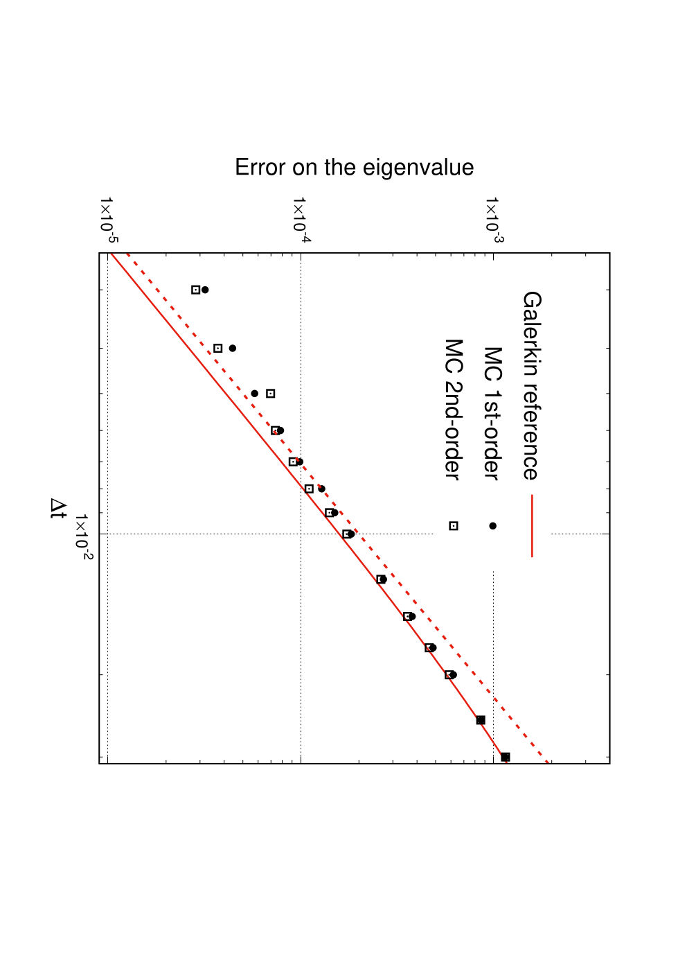
This result is important since it implies that we can approximate the eigenvalue $\lambda$ by computing $\lambda_{\Delta t}$ , which is proportional to the logarithm of the average creation of probability over a timestep $\Delta t$ (given by $Q_{\Delta t}^{W}\mathds{1}$ ) at stationarity. This is the reason why we need the coefficients $a_{k}$ to be correct up to order $p$ (i.e. $a_{k}=\lambda^{k}/k!$ ) since they represent the creation of probability of the discretized process. The estimate (46) justifies the use of population based dynamics [30, 65, 55] when the underlying continuous diffusions are discretized in time. We illustrate the error estimate (46) in the numerical simulations reported in Section 4.

Proof.

We use Lemma 5 to prove the theorem, which highlights the importance of this result in our context. In all this proof, $r_{W,\Delta t}$ denotes a smooth function which may change from line to line, but whose $C^{0}$ norm is always uniformly bounded for sufficiently small timesteps $\Delta t$ . From the definition (23) and the estimate (43),

\lambda_{\Delta t}=\frac{1}{\Delta t}\log\left(\mathrm{e}^{\Delta t\lambda_{\Delta t}}\right)=\frac{1}{\Delta t}\log\left(\mathrm{e}^{\Delta t\tilde{\lambda}_{\Delta t}}+\Delta t^{p+2}r_{W,\Delta t}\right).

Expanding $\mathrm{e}^{\Delta t\tilde{\lambda}_{\Delta t}}$ defined in (37) in powers of $\Delta t$ and recalling that $\mathcal{A}^{W}_{1}\mathds{1}=W$ ,

	$\displaystyle\lambda_{\Delta t}$	$\displaystyle=\frac{1}{\Delta t}\log\left[\int_{\mathcal{D}}\left(1+\Delta tW+\Delta t^{2}\mathcal{A}^{W}_{2}\mathds{1}+\ldots+\Delta t^{p+1}\mathcal{A}^{W}_{p+1}\mathds{1}\right)(1+\Delta t^{p}f)\,d\nu_{W}+\Delta t^{p+2}r_{W,\Delta t}\right]$
		$\displaystyle=\frac{1}{\Delta t}\log\left[1+\Delta t\lambda+\ldots+\Delta t^{p}\frac{\lambda^{p}}{p!}+\Delta t^{p+1}\int_{\mathcal{D}}\left(\mathcal{A}^{W}_{p+1}\mathds{1}+Wf\right)d\nu_{W}+\Delta t^{p+2}r_{W,\Delta t}\right],$

where we used that $\int_{\mathcal{D}}f\,d\nu_{W}=0$ and, in view of (8),

\forall\,k\in\{1,\ldots,p\},\qquad\int_{\mathcal{D}}\mathcal{A}^{W}_{k}\mathds{1}\,d\nu_{W}=\int_{\mathcal{D}}\left[\frac{(\mathcal{L}+W)^{k}}{k!}\mathds{1}\right]h_{W}\,d\nu=\int_{\mathcal{D}}\left[\frac{(\mathcal{L}^{*}+W)^{k}}{k!}h_{W}\right]d\nu=\frac{\lambda^{k}}{k!}.

(48)

Therefore,

	$\displaystyle\lambda_{\Delta t}$	$\displaystyle=\frac{1}{\Delta t}\log\left[\mathrm{e}^{\Delta t\lambda}-\sum_{k=p+2}^{+\infty}\Delta t^{k}\frac{\lambda^{k}}{k!}+\Delta t^{p+1}\int_{\mathcal{D}}\left(\mathcal{A}^{W}_{p+1}\mathds{1}-\frac{\lambda^{p+1}}{(p+1)!}+Wf\right)d\nu_{W}+\Delta t^{p+2}r_{W,\Delta t}\right]$
		$\displaystyle=\frac{1}{\Delta t}\log\left[\mathrm{e}^{\Delta t\lambda}+\Delta t^{p+1}\int_{\mathcal{D}}\left(\mathcal{A}^{W}_{p+1}\mathds{1}-\frac{\lambda^{p+1}}{(p+1)!}+Wf\right)d\nu_{W}+\Delta t^{p+2}r_{W,\Delta t}\right].$

Given that $\mathrm{e}^{\Delta t\lambda}$ is uniformly bounded for $0<\Delta t\leqslant\Delta t^{*}$ and equal to $1$ at leading order in $\Delta t$ , we obtain, by expanding the logarithm,

\lambda_{\Delta t}=\lambda+\Delta t^{p}\,\mathrm{e}^{-\Delta t\lambda}\left[\int_{\mathcal{D}}\left(\mathcal{A}^{W}_{p+1}\mathds{1}+Wf\right)d\nu_{W}-\frac{\lambda^{p+1}}{(p+1)!}\right]+\Delta t^{p+1}r_{W,\Delta t}.

The result then follows from $\mathrm{e}^{-\Delta t\lambda}=1+\Delta t\,r_{\lambda,\Delta t}$ and the definition (47) of $\lambda_{p+1}$ . ∎

3.3 TU Lemma

In the context of splitting schemes, it may be useful to relate the invariant probability measures of two numerical schemes differing by the ordering of the applied operators. This is the purpose of a result called “TU lemma” in [45], which we adapt to our context in Lemma 7. We then state a similar version of this lemma for the eigenvalues of two such schemes in Proposition 5. We will see in Section 3.4 that this last result can be combined with Theorem 3 to show that the schemes (14) and (16) both provide second order estimates of the principal eigenvalue $\lambda$ using (46), when the discretization of the process $Q_{\Delta t}$ is weakly consistent of order 2.

Lemma 7.

Consider two numerical schemes for the Feynman–Kac dynamics with associated evolution operators $Q_{\Delta t}^{W}$ and $\widetilde{Q}_{\Delta t}^{W}$ satisfying Assumption 1, and denote by $\nu_{W,\Delta t}$ and $\tilde{\nu}_{W,\Delta t}$ respectively the associated ergodic measures in the sense of Theorem 1. Assume that the evolution operators are related by two operators $T_{\Delta t}^{W}$ and $U_{\Delta t}^{W}$ , bounded on $B^{\infty}(\mathcal{D})$ , as:

\forall\,n\geqslant 1,\qquad\left(\widetilde{Q}_{\Delta t}^{W}\right)^{n}=T_{\Delta t}^{W}\left(Q_{\Delta t}^{W}\right)^{n}U_{\Delta t}^{W}.

(49)

Then, for any $\varphi\in\mathcal{S}$ ,

\int_{\mathcal{D}}\varphi\,d\tilde{\nu}_{W,\Delta t}=\frac{\displaystyle\int_{\mathcal{D}}U_{\Delta t}^{W}\varphi\,d\nu_{W,\Delta t}}{\displaystyle\int_{\mathcal{D}}U_{\Delta t}^{W}\mathds{1}\,d\nu_{W,\Delta t}}.

(50)

For the TU lemma stated in [45], the typical case of application corresponds to $Q_{\Delta t}=U_{\Delta t}T_{\Delta t}$ and $\widetilde{Q}_{\Delta t}=T_{\Delta t}U_{\Delta t}$ , with two Markov operators $T_{\Delta t}$ and $U_{\Delta t}$ . In this case, the relation (49) holds with a power $n-1$ on the right-hand side. For Feynman–Kac semigroups, $T_{\Delta t}^{W}$ and $U_{\Delta t}^{W}$ are a priori such that $T_{\Delta t}^{W}\mathds{1}\neq\mathds{1}$ and $U_{\Delta t}^{W}\mathds{1}\neq\mathds{1}$ . A typical case of interest is $Q_{\Delta t}^{W}=\mathrm{e}^{\Delta tW}Q_{\Delta t}$ and $\widetilde{Q}_{\Delta t}^{W}=Q_{\Delta t}\left(\mathrm{e}^{\Delta tW}\cdot\right)$ , in which case (49) is satisfied with $T_{\Delta t}^{W}=\mathrm{e}^{-\Delta tW}$ and $U_{\Delta t}^{W}=\mathrm{e}^{\Delta tW}$ .

Proof.

For any $\mu\in\mathcal{P}(\mathcal{D})$ and any $\varphi\in\mathcal{S}$ ,

	$\displaystyle\widetilde{\Phi}_{\Delta t,n}(\mu)(\varphi)$	$\displaystyle=\frac{\mu\left(\left(\widetilde{Q}_{\Delta t}^{W}\right)^{n}\varphi\right)}{\mu\left(\left(\widetilde{Q}_{\Delta t}^{W}\right)^{n}\mathds{1}\right)}=\frac{\mu\left(T_{\Delta t}^{W}\left(Q_{\Delta t}^{W}\right)^{n}U_{\Delta t}^{W}\varphi\right)}{\mu\left(T_{\Delta t}^{W}\left(Q_{\Delta t}^{W}\right)^{n}U_{\Delta t}^{W}\mathds{1}\right)}$
		$\displaystyle=\frac{\left(\mu T_{\Delta t}^{W}\right)\left(\left(Q_{\Delta t}^{W}\right)^{n}\mathds{1}\right)}{\left(\mu T_{\Delta t}^{W}\right)\left(\left(Q_{\Delta t}^{W}\right)^{n}U_{\Delta t}^{W}\mathds{1}\right)}\times\frac{\left(\mu T_{\Delta t}^{W}\right)\left(\left(Q_{\Delta t}^{W}\right)^{n}U_{\Delta t}^{W}\varphi\right)}{\left(\mu T_{\Delta t}^{W}\right)\left(\left(Q_{\Delta t}^{W}\right)^{n}\mathds{1}\right)}=\frac{\Phi_{\Delta t,n}(\mu_{1})(U_{\Delta t}^{W}\varphi)}{\Phi_{\Delta t,n}(\mu_{1})(U_{\Delta t}^{W}\mathds{1})},$

where $\mu_{1}\in\mathcal{P}(\mathcal{D})$ is defined by

\forall\phi\in\mathcal{S},\qquad\mu_{1}\left(\phi\right)=\frac{\displaystyle\mu\left(T_{\Delta t}^{W}\phi\right)}{\displaystyle\mu\left(T_{\Delta t}^{W}\mathds{1}\right)}.

The result then follows from the ergodic limits

\underset{n\to+\infty}{\lim}\Phi_{\Delta t,n}(\mu_{1})(\varphi)=\int_{\mathcal{D}}\varphi\,d\nu_{W,\Delta t},\qquad\underset{n\to+\infty}{\lim}\widetilde{\Phi}_{\Delta t,n}(\mu)(\varphi)=\int_{\mathcal{D}}\varphi\,d\tilde{\nu}_{W,\Delta t},

as provided by Theorem 1. ∎

In our framework, the approximate principal eigenvalue $\lambda_{\Delta t}$ is another important feature of a discretization scheme. In fact, under an additional assumption on the operators $T_{\Delta t}^{W}$ and $U_{\Delta t}^{W}$ , schemes related by (49) share the same approximate eigenvalues in the sense of (23). This is made precise in the following proposition (see Section 6.4 for the proof).

Proposition 5.

Fix a timestep $\Delta t>0$ and consider a numerical scheme for the Feynman–Kac dynamics corresponding to an evolution operator $Q_{\Delta t}^{W}$ satisfying Assumption 1, with associated invariant measure $\nu_{W,\Delta t}$ given by Theorem 1, and eigenvalue $\lambda_{\Delta t}$ defined by (23). Consider next a second scheme corresponding to an operator $\widetilde{Q}_{\Delta t}^{W}$ related to $Q_{\Delta t}^{W}$ by (49), with operators $U_{\Delta t}^{W}$ and $T_{\Delta t}^{W}$ bounded on $B^{\infty}(\mathcal{D})$ and for which there exists $\alpha>0$ such that, for any $\varphi\in\mathcal{S}$ with $\varphi\geqslant 0$ ,

\alpha\varphi\leqslant U_{\Delta t}^{W}\varphi\leqslant\alpha^{-1}\varphi,\quad\alpha\varphi\leqslant T_{\Delta t}^{W}\varphi\leqslant\alpha^{-1}\varphi.

(51)

Then, $\widetilde{Q}_{\Delta t}^{W}$ satisfies Assumption 1, and its invariant probability measure is denoted by $\tilde{\nu}_{W,\Delta t}$ . Moreover, its associated eigenvalue $\tilde{\lambda}_{\Delta t}$ defined by

\tilde{\lambda}_{\Delta t}=\frac{1}{\Delta t}\log\left[\int_{\mathcal{D}}\widetilde{Q}_{\Delta t}^{W}\mathds{1}\,d\tilde{\nu}_{W,\Delta t}\right],

(52)

is such that

\tilde{\lambda}_{\Delta t}=\lambda_{\Delta t}.

The eigenvalue $\tilde{\lambda}_{\Delta t}$ should not be mistaken in this context with the definition (37), which serves as an intermediate in the proof of Theorem 2. A careful inspection of the proof shows that it would be possible to consider a slightly different assumption (51).

Remark 4.

Although Proposition 5 may look odd at first sight, it has a natural interpretation in terms of matrices. Indeed, if $A\in\mathbb{R}^{n\times n}$ and $B\in\mathbb{R}^{n\times n}$ are two square matrices with nonnegative entries, the products $AB$ and $BA$ share the same real principal eigenvalue. One can show this by the following argument. For any matrix $M\in\mathbb{R}^{n\times n}$ with nonnegative entries, the spectral radius

\rho(M)=\underset{n\to+\infty}{\lim}\|M^{n}\|^{\frac{1}{n}}

is an eigenvalue of $M$ (see [64]). This eigenvalue is the equivalent of the principal eigenvalue for the operator $\mathcal{L}+W$ since it is the eigenvalue of the matrix $M$ with the largest real part. It is easy to see that $\rho(AB)=\rho(BA)$ by noting that

\rho(AB)=\underset{n\to+\infty}{\lim}\|(AB)^{n}\|^{\frac{1}{n}}=\underset{n\to+\infty}{\lim}\|A(BA)^{n-1}B\|^{\frac{1}{n}}\leqslant\underset{n\to+\infty}{\lim}\|A\|^{\frac{1}{n}}\|(BA)^{n-1}\|^{\frac{1}{n}}\|B\|^{\frac{1}{n}}=\rho(BA).

This leads to $\rho(AB)\leqslant\rho(BA)$ , and, by symmetry, $\rho(BA)\leqslant\rho(AB)$ ; hence $\rho(AB)=\rho(BA)$ . In the same way, evolution operators related by (49) share the same principal eigenvalue even though, a priori, they do not admit the same invariant probability measures. The proof of Proposition 5, presented in Section 6.4, follows a path similar to the one used here for matrices.

3.4 Second order schemes

We now turn to second order schemes for Feynman–Kac dynamics. They are the most interesting ones in practice, since they can provide an important improvement in the accuracy for a relatively cheap computational overhead. Moreover, in our case, they can be straightforwardly built from second order schemes for the dynamics (1), as a consequence of Theorem 2.

Lemma 8.

Suppose that (25) and (27) hold with the following expansion for $Q_{\Delta t}$ :

\forall\,\varphi\in\mathcal{S},\qquad Q_{\Delta t}\varphi=\varphi+\Delta t\mathcal{L}\varphi+\Delta t^{2}\frac{\mathcal{L}^{2}\varphi}{2}+\Delta t^{3}\mathcal{A}_{3}\varphi+\Delta t^{4}\mathcal{R}_{\Delta t}\varphi,

(53)

where $\mathcal{A}_{3}$ is a differential operator with smooth coefficients and $\mathcal{R}_{\Delta t}$ satisfies (27). Then the operator $Q_{\Delta t}^{W}$ defined by

\forall\,\varphi\in\mathcal{S},\qquad Q_{\Delta t}^{W}\varphi=\mathrm{e}^{\frac{\Delta t}{2}W}Q_{\Delta t}\left(\mathrm{e}^{\frac{\Delta t}{2}W}\varphi\right),

satisfies Assumption 2 with $p=2$ :

\forall\,\varphi\in\mathcal{S},\qquad Q_{\Delta t}^{W}\varphi=\varphi+\Delta t(\mathcal{L}+W)\varphi+\Delta t^{2}\frac{(\mathcal{L}+W)^{2}\varphi}{2}+\Delta t^{3}\mathcal{A}^{W}_{3}\varphi+\Delta t^{4}\mathcal{R}_{W,\Delta t}\varphi,

(54)

where

\mathcal{A}^{W}_{3}\varphi=\mathcal{A}_{3}\varphi+\frac{W^{3}\varphi}{6}+\frac{\mathcal{L}(W^{2}\varphi)}{8}+\frac{\mathcal{L}^{2}(W\varphi)}{4}+\frac{W\mathcal{L}^{2}\varphi}{4}+\frac{W\mathcal{L}(W\varphi)}{4}+\frac{W^{2}\mathcal{L}\varphi}{8},

and $\mathcal{R}_{W,\Delta t}$ satisfies (27).

The interpretation of this result is the following: when we have a scheme consistent at order 2 for the dynamics with $W=0$ , we immediately obtain a second order scheme for the Feynman–Kac dynamics by using the corresponding Markov chain and a trapezoidal rule for the time integral in the exponential. Thanks to the consistency at order one ( $\mathcal{A}^{W}_{1}=\mathcal{L}+W$ ) and Propositions 1 and 4, the assumptions of Theorems 2 and 3 are immediately satisfied with $p=2$ .

Proof.

The expression of $\mathcal{A}^{W}_{3}$ can be obtained by a direct computation or with the Baker-Campbell-Hausdorff formula (see [32]), which is a convenient way to perform the algebra allowing to make precise the various terms in expansions in powers of $\Delta t$ . Let us sketch how this is done, and refer to [45] for strategies of proof in order to make the expansions below rigorous. First,

Q_{\Delta t}=\mathrm{e}^{\Delta t\mathcal{L}}+\Delta t^{3}\left(\mathcal{A}_{3}-\frac{\mathcal{L}^{3}}{6}\right)+...

and, by the Baker-Campbell-Hausdorff formula,

\mathrm{e}^{\Delta tW/2}\mathrm{e}^{\Delta t\mathcal{L}}\mathrm{e}^{\Delta tW/2}=\mathrm{e}^{S_{\Delta t}},\qquad S_{\Delta t}=\Delta t(\mathcal{L}+W)+\frac{\Delta t^{3}}{12}\left(-\frac{1}{2}\big[W,[W,\mathcal{L}]\big]+\big[\mathcal{L},[\mathcal{L},W]\big]\right),

where $[A,B]=AB-BA$ denotes the commutator of two operators $A$ and $B$ . Therefore,

\mathrm{e}^{\Delta tW/2}\mathrm{e}^{\Delta t\mathcal{L}}\mathrm{e}^{\Delta tW/2}=\mathrm{Id}+\Delta t(\mathcal{L}+W)+\frac{\Delta t^{2}}{2}(\mathcal{L}+W)^{2}+\frac{\Delta t^{3}}{6}(\mathcal{L}+W)^{3}+\frac{\Delta t^{3}}{12}\left(-\frac{1}{2}\big[W,[W,\mathcal{L}]\big]+\big[\mathcal{L},[\mathcal{L},W]\big]\right)+...

The conclusion then follows from

\mathrm{e}^{\Delta tW/2}Q_{\Delta t}\mathrm{e}^{\Delta tW/2}=\mathrm{e}^{\Delta tW/2}\mathrm{e}^{\Delta t\mathcal{L}}\mathrm{e}^{\Delta tW/2}+\Delta t^{3}\left(\mathcal{A}_{3}-\frac{\mathcal{L}^{3}}{6}\right)+...

upon developping the commutators. ∎

When we are interested in the computation of the principal eigenvalue with Theorem 3, we can in fact show that the left-point integration (14) is sufficient for $\lambda_{\Delta t}$ to be correct at order 2 if $Q_{\Delta t}$ is consistent at order 2 (i.e. (53) holds). In particular, the discretization scheme for the Feynman–Kac dynamics need not be consistent at order 2 for the eigenvalue to be correct at order 2 (in the same way that the invariant probability measure for discretizations of ergodic SDEs can be correct at order 2 even if the discretization itself is only weakly consistent at order 1, see [3, 45, 46]). This consequence of Proposition 5 is made precise in the following proposition.

Proposition 6.

Consider an evolution operator $Q_{\Delta t}$ with the following familly of discretizations for the Feynman–Kac dynamics:

Q_{\Delta t}^{W,\delta}=\mathrm{e}^{(1-\delta)W\Delta t}Q_{\Delta t}\mathrm{e}^{\delta W\Delta t},\quad\delta\in[0,1].

Suppose that Assumption 1 holds for at least one of these schemes, and denote by $\lambda_{\Delta t}^{\delta}$ their associated eigenvalues as in (23). Then, $\lambda_{\Delta t}^{\delta}$ is independent of $\delta$ . Moreover, when $Q_{\Delta t}$ satisfies (53), the eigenvalue $\lambda_{\Delta t}^{\delta}$ satisfies (46) with $p=2$ for any $\delta\in[0,1]$ .

Proof.

The proof is a simple application of Proposition 5. Consider the scheme $Q_{\Delta t}^{W,\delta}$ for a fixed $\delta\in[0,1]$ and the scheme $\widetilde{Q}_{\Delta t}^{W}=\mathrm{e}^{\Delta t\frac{W}{2}}Q_{\Delta t}\mathrm{e}^{\Delta t\frac{W}{2}}$ , which corresponds to a trapezoidal approximation of the integral. We can assume without loss of generality that $\widetilde{Q}_{\Delta t}^{W}$ satisfies Assumption 1. Then, $Q_{\Delta t}^{W,\delta}$ is related to $\widetilde{Q}_{\Delta t}^{W}$ through (49) for the corresponding operators:

U_{\Delta t}^{W}=\mathrm{e}^{\left(\delta-\frac{1}{2}\right)\Delta tW},\quad T_{\Delta t}^{W}=\mathrm{e}^{\left(\frac{1}{2}-\delta\right)\Delta tW}.

The operators $U_{\Delta t}^{W}$ and $T_{\Delta t}^{W}$ are bounded on $B^{\infty}(\mathcal{D})$ and satisfy (51) with $\alpha=\mathrm{e}^{-\Delta t\|W\|_{B^{\infty}(\mathcal{D})}/2}$ . Therefore, by Proposition 5, the eigenvalue $\lambda_{\Delta t}^{\delta}$ associated to $Q_{\Delta t}^{W,\delta}$ is equal to $\tilde{\lambda}_{\Delta t}$ , the eigenvalue associated to $\widetilde{Q}_{\Delta t}^{W}$ , and thus does not depend on $\delta$ . Moreover, by Lemma 8, if $Q_{\Delta t}$ satisfies (53), $\widetilde{Q}_{\Delta t}^{W}$ satisfies the assumptions of Theorem 3 with $p=2$ . This shows that the eigenvalue $\lambda_{\Delta t}^{\delta}$ satisfies (46) with $p=2$ whatever the integration rule (i.e. for any $\delta\in[0,1]$ ). ∎

Remark 5.

Proposition 6 shows that the eigenvalue $\lambda_{\Delta t}$ can be correct at order two even though the scheme only has weak order one. One may wonder whether it is also possible to have second order convergence on the invariant measure when $Q_{\Delta t}$ corresponds to a scheme of weak order one. As mentioned in Section 3.1.1 this is the case when $W=0$ , see the examples in [45]. Perturbative arguments for small $W$ however show that this extra cancellation on the invariant measure cannot happen for a non-constant $W$ , see [26].

4 Numerical application

The goal of this section is to illustrate the error estimates presented in Section 3 on a toy example. For this, we consider (1) over the one dimensional torus $\mathcal{D}=\mathbb{T}$ with possibly non-gradient drifts:

dq_{t}=(-V^{\prime}(q_{t})+\gamma)\,dt+\sigma\,dB_{t},

(55)

where $V$ is a smooth potential and $\gamma\in\mathbb{R}$ . Let us emphasize that a constant force is not the gradient of a smooth periodic function. We first make precise in Section 4.1 the Monte Carlo algorithm used to compute the Feynman–Kac averages. We next describe in Section 4.2 a Galerkin method to compute reference values for the properties of interest. Note that such a discretization method can be used only for low-dimensional systems; but, when it can be used, it typically provides more accurate results than stochastic methods. Finally, we present our numerical results in Section 4.3.

4.1 Monte Carlo discretization

Discretization of the underlying SDE.

The Euler-Maruyama discretization of the dynamics (55) is given by:

q^{n+1}=q^{n}+\big(-V^{\prime}(q^{n})+\gamma\big)\Delta t+\sigma\sqrt{\Delta t}\,G^{n},

(56)

where $G^{n}$ are independent and identically distributed one-dimensional standard Gaussian variables. It is well known that this scheme is weakly consistent of order one (see for instance [54, 9]). In order to test our results on a second order scheme, we use a discretization proposed e.g. in [1, 72, 25, 69]:

q^{n+1}=q^{n}-V^{\prime}\left(q^{n}+\left(-V^{\prime}(q^{n})+\gamma\right)\frac{\Delta t}{2}+\frac{1}{2}\sigma\sqrt{\Delta t}\,G^{n}\right)\Delta t+\gamma\Delta t-\frac{\sigma^{2}}{8}V^{\prime\prime\prime}(q^{n})\Delta t^{2}+\sigma\sqrt{\Delta t}\,G^{n}.

(57)

It can be proved that this scheme is of weak order $2$ .

Weighted dynamics.

Once the underlying SDE has been discretized, a Monte Carlo scheme for approximating the associated Feynman–Kac semigroup (15) has to be devised. Several methods have been succefully applied in order to compute Feynman–Kac averages, generally referred to as Sequential Monte Carlo or Population Monte Carlo methods [21, 10, 47]. For simplicity and numerical efficiency, we present here a population method with multinomial resampling. More precisions on this familly of algorithms are available in [21], see also [47, Chapter 6] in the context of free energy computation and [34] in the context of Diffusion Monte Carlo.

The algorithm relies on a dynamics run over a set of replicas of the system. At each step, the replicas are updated according to the dynamics prescribed by the evolution operator $Q_{\Delta t}$ , and are assigned an importance weight depending on the choice of discretization rule for the integral. The replicas are then resampled following a multinomial distribution with their respective weights, before computing the desired averages. This technique prevents the variance of the estimator to increase exponentially in time, a common problem when computing directly quantities such as (15). We now make precise the algorithm.

Consider a population of $M$ replicas $(q_{m})_{m=1,\ldots,M}$ initially distributed according to some probability measure $\mu^{\otimes_{M}}$ over $\mathcal{D}^{M}$ and evolving through a Markov kernel $Q_{\Delta t}$ with timestep $\Delta t>0$ . We denote by $\chi_{\Delta t}:\mathcal{D}\times\mathcal{D}\to\mathbb{R}$ a weight function to be chosen later on. The algorithm consists in repeating for each time $0\leqslant n<N_{\mathrm{iter}}$ the following steps:

(1)

For $m\in\{1,\ldots,M\}$ , evolve the $m^{\mathrm{th}}$ replica as $\tilde{q}_{m}^{n+1}\sim Q_{\Delta t}(q_{m}^{n},\cdot)$ ;
(2)

Compute the weight of each replica as $w_{m}^{n}=\mathrm{e}^{\chi_{\Delta t}(q_{m}^{n},\tilde{q}_{m}^{n+1})}$ ;
(3)

Compute the total creation of mass as

$P^{n}=\sum_{m=1}^{M}w_{m}^{n},$

and the normalized probability vector $p^{n}\in\mathbb{R}^{m}$ with components $p_{m}^{n}=w_{m}^{n}/P^{n}$ , for $m\in\{1,\ldots,M\}$ ;
(4)

Resample the replicas $(\tilde{q}_{m}^{n+1})_{m=1}^{M}$ according to the multinomial distribution associated with $p^{n}$ , which defines a new set of replicas $(q_{m}^{n+1})_{m=1}^{M}$ ;
(5)

Compute the estimator

$\widehat{\varphi}_{n}=\frac{1}{M}\sum_{m=1}^{M}\varphi(q_{m}^{n+1}).$

Until now, we did not specify the choice of function $\chi_{\Delta t}$ , which depends on the discretization rule for the integral in (3). In practice, given a discretization of the SDE characterized by an operator $Q_{\Delta t}$ , we use the schemes defined by the left point integration $\mathrm{e}^{\Delta tW}Q_{\Delta t}$ , and by the trapezoidal integration $\mathrm{e}^{\Delta t\frac{W}{2}}Q_{\Delta t}\mathrm{e}^{\Delta t\frac{W}{2}}$ . They correspond respectively to the choices:

\chi_{\Delta t}(q,q^{\prime})=\Delta t\,W(q)\quad\mbox{and}\quad\chi_{\Delta t}(q,q^{\prime})=\Delta t\left(\frac{W(q)+W(q^{\prime})}{2}\right).

(58)

The principal eigenvalue of the operator $\mathcal{L}+W$ is then estimated with (46) through

\lambda_{\Delta t}=\frac{1}{\Delta t}\log\left[\int_{\mathcal{D}}Q_{\Delta t}^{W}\mathds{1}\ d\nu_{W,\Delta t}\right]\approx\frac{1}{\Delta t}\log\left[\frac{1}{N_{\mathrm{iter}}}\sum_{n=0}^{N_{\mathrm{iter}}-1}P^{n}\right],

(59)

while the average of $\varphi$ is estimated by

\int_{\mathcal{D}}\varphi\,d\nu_{W,\Delta t}\approx\frac{1}{N_{\mathrm{iter}}}\sum_{n=0}^{N_{\mathrm{iter}}-1}\widehat{\varphi}_{n},

(60)

where the $\approx$ sign indicates the approximation arising from the finiteness of the number $M$ of replicas and of the number $N_{\mathrm{iter}}$ of steps. We do not take these errors into account and ensure numerically that they are sufficiently small in our simulations to observe the bias due to the timestep (this bias being quite small in practice, this also motivates to study a one-dimensional model, see the numerical results below). The reader interested in the convergence rates of this type of algorithm when $M\to+\infty$ and $N_{\mathrm{iter}}\to+\infty$ is refered e.g. to [13, 21, 61, 23].

4.2 Galerkin discretization

We now make precise the Galerkin method that can be used to estimate $\lambda_{\Delta t}$ and $\int_{\mathcal{D}}\varphi\,d\nu_{W,\Delta t}$ . This discretization provides reference values for the Monte Carlo method described in Section 4.1. In particular, when $V=0$ and $\gamma=0$ , the two methods should give the same result since the Euler scheme (56) is exact in law in this specific case.

Choice of the Galerkin basis.

Since we work with periodic functions, we consider the Galerkin subspace $\mathrm{Span}\{e_{-N},\ldots,e_{N}\}$ with

e_{n}(q)=\mathrm{e}^{2\mathrm{i}\pi nq}.

The generator of the SDE (55) reads

\mathcal{L}=(-V^{\prime}+\gamma)\partial_{q}+\frac{\sigma^{2}}{2}\partial_{q}^{2}.

The operators $\mathcal{L}^{\dagger}$ and $W$ are represented in this Galerkin subspace by the matrices $L^{N}$ , $B^{N}\in\mathbb{C}^{(2N+1)\times(2N+1)}$ defined as

\forall\,m,n\in\{-N,\ldots,0,\ldots,N\},\qquad L_{n,m}^{N}=\int_{\mathcal{D}}e_{n}(\mathcal{L}^{\dagger}e_{m}),\quad B_{n,m}^{N}=\int_{\mathcal{D}}We_{n}e_{m}.

The value of $N$ is chosen sufficiently large for all results to be converged with respect to this parameter. The only source of error in the quantities we compute then arises from the finiteness of the timestep $\Delta t>0$ , and possibly numerical quadratures to evaluate certain integrals. Our experience shows that $N=30$ is already sufficient for the applications described in Section 4.3.

References quantities for $\Delta t=0$ .

The invariant probability measure $\nu_{W}$ satisfies the eigenvalue problem $(\mathcal{L}^{\dagger}+W)\nu_{W}=\lambda\nu_{W}$ . We compute a reference approximation $\lambda^{N}_{0}$ to $\lambda$ by computing the eigenvalue of $L^{N}+B^{N}$ with the largest real part:

(L^{N}+B^{N})\mathcal{V}_{W,0}^{N}=\lambda_{0}^{N}\mathcal{V}_{W,0}^{N}.

The associated eigenvector allows to construct the following approximation of $\nu_{W}$ :

\nu_{W,0}^{N}=\sum_{k=-N}^{N}[\mathcal{V}_{W,0}^{N}]_{k}e_{k}.

The normalization condition $[\mathcal{V}_{W,0}^{N}]_{0}=1$ ensures that $\nu_{W,0}^{N}$ has a total mass 1. Averages of observables $\varphi$ are then estimated by computing the following integral

\int_{\mathcal{D}}\varphi(q)\nu_{W,0}^{N}(q)\,dq

using a one-dimensional quadrature rule.

Reference quantities for $\Delta t>0$ .

We next approximate the evolution operators of the first order scheme $\mathrm{e}^{\Delta tW}Q_{\Delta t}$ and of the second order one $\mathrm{e}^{\Delta t\frac{W}{2}}Q_{\Delta t}\mathrm{e}^{\Delta t\frac{W}{2}}$ , respectively as

Q_{\Delta t,1}^{W,N}=\mathrm{e}^{\Delta tB^{N}}\mathrm{e}^{\Delta tL^{N}},\qquad Q_{\Delta t,2}^{W,N}=\mathrm{e}^{\Delta t\frac{B^{N}}{2}}\mathrm{e}^{\Delta tL^{N}}\mathrm{e}^{\Delta t\frac{B^{N}}{2}}.

(61)

For each value of $\Delta t$ , we construct the above matrices, and compute their respective principal eigenvalues $\Lambda_{\Delta t,1}^{N}$ , $\Lambda_{\Delta t,2}^{N}$ and eigenvectors $\mathcal{V}_{W,\Delta t}^{N,1}$ , $\mathcal{V}_{W,\Delta t}^{N,2}\in\mathbb{C}^{2N+1}$ by diagonalization (still with the normalization condition $[\mathcal{V}_{W,\Delta t}^{N,j}]_{0}=1$ for $j=1,2$ ). We then consider the following approximations of the principal eigenvalue $\lambda$ of the Feynman–Kac operator $\mathcal{L}+W$ , based on (46):

\lambda_{\Delta t,1}^{N}=\frac{1}{\Delta t}\log\Lambda_{\Delta t,1}^{N},\qquad\lambda_{\Delta t,2}^{N}=\frac{1}{\Delta t}\log\Lambda_{\Delta t,2}^{N}.

(62)

Averages of $\varphi$ with respect to the invariant probability measure are approximated by the following quantity, using the eigenvectors $\mathcal{V}_{W,\Delta t}^{N,1}$ and $\mathcal{V}_{W,\Delta t}^{N,2}$ : for $j=1,2$ ,

\int_{\mathcal{D}}\varphi(q)\nu_{W,\Delta t}^{N,j}(q)\,dq,\qquad\nu_{W,\Delta t}^{N,j}=\sum_{k=-N}^{N}[\mathcal{V}_{W,\Delta t}^{N,j}]_{k}e_{k}.

(63)

In view of Theorem 2, we expect the average of $\varphi$ to converge linearly in $\Delta t$ for the first order scheme when $\Delta t\to 0$ , and quadratically for the second order scheme. We also use the TU-lemma to show that, by appropriately correcting the first order scheme, we recover the same results as for the second order scheme. More precisely, we apply (50) with $U_{\Delta t}^{W}=\mathrm{e}^{\Delta t\frac{W}{2}}$ , which leads to the following approximation of the average (estimated in practice using a numerical quadrature):

\frac{\displaystyle\int_{\mathcal{D}}\mathrm{e}^{\Delta t\frac{W(q)}{2}}\varphi(q)\nu_{W,\Delta t}^{N,1}(q)\,dq}{\displaystyle\int_{\mathcal{D}}\mathrm{e}^{\Delta t\frac{W(q)}{2}}\nu_{W,\Delta t}^{N,1}(q)\,dq}.

(64)

On the other hand, from Proposition 6, the eigenvalues $\lambda_{\Delta t,1}^{N}$ and $\lambda_{\Delta t,2}^{N}$ should be equal, and therefore $\lambda_{\Delta t,1}^{N}$ need not be corrected.

4.3 Numerical results

Zero-potential case.

We first choose $V=0$ , $\sigma=\sqrt{2}$ , $W(q)=(\cos(2\pi q))^{2}$ and $\varphi(q)=\exp(\cos(2\pi q))$ . As mentioned earlier, in this case, the Euler scheme (56) is exact in law, so that the only source of error arises from the integration of the exponential weight. We consider the dynamics represented by the operator $\mathrm{e}^{\Delta tW}Q_{\Delta t}$ and $\mathrm{e}^{\Delta t\frac{W}{2}}Q_{\Delta t}\mathrm{e}^{\Delta t\frac{W}{2}}$ with $Q_{\Delta t}=\mathrm{e}^{\Delta t\mathcal{L}}$ , and first compare the results of the Galerkin discretization discussed in Section 4.2. The results reported in Figure 1 confirm our predictions: the averages of $\varphi$ converge at first and second order for the first order and second order Galerkin schemes respectively; while the eigenvalues are the same, as expected from Proposition 6, and so both converge at second order. In this case, the numerical method based on (46) is therefore more accurate than the one based on averaging $W$ with (35) to compute the principal eigenvalue $\lambda$ , which would lead to errors of order 1 in the timestep (numerical results not shown here).

Refer to caption — (a) Convergence of the eigenvalue.

We next consider the Monte Carlo scheme presented in Section 4.1, taking $M=5\times 10^{4}$ and an integration time $T=5\times 10^{2}$ , with $N_{\mathrm{iter}}=\lfloor\frac{T}{\Delta t}\rfloor$ for each timestep $\Delta t$ . We use half of the time for burn-in, and average in time over the second half of the simulation. Moreover, for each value of $\Delta t$ , we run 30 realizations in order to reduce the variance of the estimator and to estimate error bars on the Monte Carlo estimates (not displayed on the pictures). The choice of the function $\chi_{\Delta t}$ depends on the scheme through (58). We compare in Figure 2 the results of the Monte Carlo algorithm with the Galerkin approximation, which serves as a reference. The agreement is very good, up to small errors arising from the finiteness of the population and of the simulation time. This result was expected since, given that the integration by the Euler scheme is exact in law in this case, the Monte Carlo method must match exactly the Galerkin approximation provided $N$ , $N_{\rm iter}$ and $M$ are all sufficiently large.

Situation with a strong potential.

We next show an application with a non-zero drift by setting $V(q)=\cos(2\pi q)$ and $\gamma=1$ . Let us recall that this dynamics is non-reversible since a constant function is not the gradient of a smooth periodic potential. The other parameters are left unchanged. Concerning the Galerkin approximation, we consider the two schemes described in Section 4.2, and characterized by the matrices defined in (61). For these schemes, the eigenvalues are the same and converge at second order (so we only consider one scheme), while the averages of $\varphi$ converge at first and second order respectively.

For the Monte Carlo algorithm described in Section 4.1, we consider the three following schemes:

•

$Q_{\Delta t}$ is discretized with the Euler scheme (56), and $\chi_{\Delta t}(q,q^{\prime})=\Delta tW(q)$ is chosen as the left point integration; in this case, the eigenvalue and the average of $\varphi$ converge at order one, so the scheme is referred to as first order.
•

$Q_{\Delta t}$ is discretized with the second order scheme (57), and we set $\chi_{\Delta t}(q,q^{\prime})=\Delta tW(q)$ ; in this case, the eigenvalue converges at second order whereas the average of $\varphi$ converges at first order only, so the scheme is referred to as hybrid scheme.
•

$Q_{\Delta t}$ is discretized with the second order scheme (57), and we set $\chi_{\Delta t}(q,q^{\prime})=\Delta t\left(W(q)/2+W(q^{\prime})/2\right)$ , which corresponds to a trapezoidal rule for the time integral; in this case, both the eigenvalue and the average of $\varphi$ converge at order two, so we refer to this scheme as second order.

We present the numerical results obtained with the various schemes we consider in Figures 3 (eigenvalues) and 4 (averages of $\varphi$ ):

•

Concerning the eigenvalues computed with the Monte Carlo method, we indeed observe first order convergence for the first order scheme, and second order convergence for the hybrid and second order schemes. In particular, the results of the hybrid and the second order scheme are exactly the same. The Galerkin method also converges at second order, but with a much smaller prefactor. This is due to the fact that in this case most of the error is due to the discretization of the dynamics rather than the discretization of the time integral.
•

Concerning the average of $\varphi$ , the first order scheme converges at order one, while the hybrid and second order scheme converge at order two. We would have expected the hybrid scheme to converge at first order but, once again, this is due to the fact that most of the error is due to the discretization of the dynamics, and not to the time integral – as shown by the results of the Galerkin method, which amounts to observing the error due to the discretization of the time integral only. We indeed observe first and second order convergence for the Galerkin approximation, but we see that the error is orders of magnitude smaller than the one of the Monte Carlo approximation. This explains why the Monte Carlo hybrid and second order schemes seem to provide the same results.

Situation with a weak potential.

In order to obtain a better trade-off between the error due to the discretization of the dynamics and of the time integral, we run simulations with the same parameters as in the previous situation but with a smaller potential energy $V(q)=0.02\cos(2\pi q)$ . The results are the following:

•

All the eigenvalues now seem to converge at second order (see Figure 5 (a)). This is due to the fact that the error due to the discretization of the dynamics is very small, and that the discretization of the time integral, which gives the dominant error term, always leads to an effective second order convergence.
•

The behaviour of the average of $\varphi$ is more interesting (see Figure 5 (b)). The Galerkin first and second order schemes provide first and second order convergence respectively. The hybrid scheme exhibits a first order convergence, that matches the Galerkin first order scheme for small timesteps. This result can be expected since the two schemes match at order one. The first order scheme also converges at first order but with a larger prefactor, which is due to the discretization of the dynamics. On the other hand, the second order Monte Carlo scheme converges at second order, like the Galerkin second order scheme.

Conclusion.

The numerical applications we presented show the validity of our analysis on a simple test case. However, we observe numerically that the prefactor of the leading error term depends on the choice of parameters. This has the consequence that some schemes may effectively seem to exhibit an improved order of convergence than expected, while they actually have a small prefactor at leading order, depending on the discretization at hand. This observation also motivates the study of a one-dimensional model: not only can the Galerkin discretization be made sufficiently accurate by considering a very large number of basis functions, but we can also run sufficiently long Monte Carlo simulations in order for the statistical error to be negligible compared to the bias arising from the time step discretization. Although the order of convergence would be harder to observe for higher dimensional systems, the framework is still applicable and we refer to [48] and references therein for examples in high dimension.

5 Possible extensions

The analysis and simulations we performed in this work were done for SDEs with a non-degenerate noise on a torus. We however believe that most of our results could be extended to more general settings. The first issue is to study the long time behaviour of Feynman–Kac dynamics and their discretizations when considering unbounded configuration spaces and/or SDEs with degenerate noise such as inertial Langevin dynamics. We recently addressed this problem in [27] by using weighted function space in the spirit of [33]. This provides criteria in terms of growth conditions on $b$ and $W$ for extending Proposition 2 and Theorem 1, for instance, and Hörmander-type conditions for dynamics with degenerate noise.

Since the long time behaviour of unbounded dynamics has been studied, we would like to extend the error estimates on the ergodic properties of the dynamics presented in Section 3 in this unbounded setting. However, in the functional framework of [27], the stability property (Assumption 3), which is crucial for our analysis to hold, should be rephrased as the invariance of a functional space (containing unbounded functions) under the action of $h_{W}^{-1}(\mathcal{L}^{*}+W-\lambda)^{-1}(h_{W}\cdot)$ . In the case $W=0$ , which does not involve the eigenvector $h_{W}$ (since $h_{0}=\mathds{1}$ ), this is already a quite technical result to obtain (see [42, 43]). Here, the presence of the eigenvector $h_{W}$ adds a significant difficulty, which leaves the situation open.

Finally, in the context of large deviations, one is often interested in computing the rate function, which is the Fenchel transform of the eigenvalue $\lambda$ associated to a particular function $W$ , see [14]. It is an interesting and non-trivial problem to transpose our error estimates on $\lambda$ to error estimates on the rate function.

6 Proofs

6.1 Proof of the results of Section 2.1

Let us first give a result which shows that it suffices to prove Proposition 2 for probability measures which admit a positive and bounded density with respect to the Lebesgue measure. This results relies on the regularizing properties of the underlying diffusion.

Lemma 9.

For any $\alpha>0$ , denote by $\mathcal{P}_{\alpha}(\mathcal{D})$ the subspace of probability measures which admit a smooth density with respect to the Lebesgue measure, and whose density is bounded below by $\alpha>0$ and bounded above by $1/\alpha$ . Then there exists $\alpha_{*}>0$ such that $\Phi_{1}(\mu)\in\mathcal{P}_{\alpha_{*}}(\mathcal{D})$ for any $\mu\in\mathcal{P}(\mathcal{D})$ .

Proof.

Note that, for any $\varphi\in\mathcal{S}$ ,

\left(P_{t}^{W}\varphi\right)(q)=\int_{\mathcal{D}}p_{t}^{W}(q,q^{\prime})\varphi(q^{\prime})\,dq^{\prime},

where $p_{t}^{W}$ is the integral kernel of the semigroup $\mathrm{e}^{t(\mathcal{L}+W)}$ . By parabolic regularity (see for instance [24]), the integral kernel is smooth for any $t>0$ . It is also positive when $W=0$ by the irreducibility properties of the underlying non-degenerate diffusion: there exists $\eta>0$ such that (setting $t=1$ )

\forall\,(q,q^{\prime})\in\mathcal{D}^{2},\qquad\eta\leqslant p_{1}^{0}(q,q^{\prime})\leqslant\frac{1}{\eta}.

Given that $W$ is bounded, a similar property holds for $p_{t}^{W}$ : there exists $\alpha>0$ such that

\forall\,(q,q^{\prime})\in\mathcal{D}^{2},\qquad\sqrt{\alpha}\leqslant p_{1}^{W}(q,q^{\prime})\leqslant\frac{1}{\sqrt{\alpha}}.

Since, for any bounded measurable function $\varphi$ ,

\Phi_{1}(\mu)(\varphi)=\frac{\mu(P_{1}^{W}\varphi)}{\mu(P_{1}^{W}\mathds{1})}=\frac{1}{\mu(P_{1}^{W}\mathds{1})}\int_{\mathcal{D}}\int_{\mathcal{D}}\varphi(q^{\prime})p_{1}^{W}(q,q^{\prime})\,\mu(dq)dq^{\prime},

it follows that $\Phi_{1}(\mu)$ has a smooth density with respect to the Lebesgue measure, denoted by $F_{1,\mu}$ :

F_{1,\mu}(q)=\frac{1}{\mu(P_{1}^{W}\mathds{1})}\int_{\mathcal{D}}p_{1}^{W}(q^{\prime},q)\,\mu(dq^{\prime}).

Moreover, since $\mu(P_{1}^{W}\mathds{1})\geqslant\sqrt{\alpha}$ , it holds

\alpha\leqslant F_{1,\mu}\leqslant\frac{1}{\alpha},

which gives the claimed result. ∎

We can now provide the proof of Proposition 2.

Proof of Proposition 2.

In view of the semigroup property $\Phi_{t}(\mu)=\Phi_{t-1}(\Phi_{1}(\mu))$ when $t\geqslant 1$ , it is sufficient by Lemma 9 to prove the result for measures $\mu\in\mathcal{P}_{\alpha}(\mathcal{D})$ , where $\alpha>0$ . The proof is conducted in two steps: we first prove a convergence result for the linear semigroup $P_{t}^{W-\lambda}$ in $L^{2}(\nu)$ and any times $t\geqslant 0$ , and then rely on the fact that any probability measure in $\mathcal{P}_{\alpha}(\mathcal{D})$ is equivalent to $\nu$ to obtain (10).

Introduce the projector (different from the one defined in (39))

\widehat{\Pi}_{W}\varphi=\varphi-\hat{h}_{W}\frac{\big\langle\varphi,h_{W}\big\rangle_{L^{2}(\nu)}}{\left\langle\hat{h}_{W},h_{W}\right\rangle_{L^{2}(\nu)}}=\varphi-\hat{h}_{W}\frac{\int_{\mathcal{D}}\varphi\,d\nu_{W}}{\int_{\mathcal{D}}\hat{h}_{W}\,d\nu_{W}}.

A simple computation shows that $\widehat{\Pi}_{W}$ commutes with $\mathcal{L}+W$ and $P_{t}^{W-\lambda}$ . It is easily seen that the spectrum of the operator $\widehat{\Pi}_{W}(\mathcal{L}+W-\lambda)\widehat{\Pi}_{W}$ is

\sigma(\mathcal{L}+W-\lambda)\setminus\{0\}\subset\Big\{z\in\mathbb{C},\,\mathrm{Re}(z)\leqslant-\delta_{W}\Big\},

and that the associated semigroup satisfies $\mathrm{e}^{t\widehat{\Pi}_{W}(\mathcal{L}+W-\lambda)\widehat{\Pi}_{W}}=P_{t}^{W-\lambda}\widehat{\Pi}_{W}$ . By the Hille–Yosida theorem (see for instance [57, 8]), there exists therefore a constant $C>0$ such that, for any $\varphi\in L^{2}(\nu)$ ,

\forall\,t\geqslant 0,\qquad\left\|P_{t}^{W-\lambda}\widehat{\Pi}_{W}\varphi\right\|_{L^{2}(\nu)}\leqslant C\,\mathrm{e}^{-\delta_{W}t}\|\varphi\|_{L^{2}(\nu)}.

(65)

We now show that (65) implies the convergence result (10) for the class of probability measures $\mathcal{P}_{\alpha}(\mathcal{D})$ . For a given $\mu\in\mathcal{P}_{\alpha}(\mathcal{D})$ and $\varphi\in L^{2}(\nu)$ ,

	$\displaystyle\mu\left[\left\|P_{t}^{W-\lambda}\widehat{\Pi}_{W}\varphi\right\|\right]$	$\displaystyle=\int_{\mathcal{D}}\left\|P_{t}^{W-\lambda}\widehat{\Pi}_{W}\varphi\right\|\,d\mu\leqslant\frac{1}{\alpha}\int_{\mathcal{D}}\left\|P_{t}^{W-\lambda}\widehat{\Pi}_{W}\varphi\right\|\,\frac{d\nu}{\inf_{\mathcal{D}}\nu}$
		$\displaystyle\leqslant\frac{1}{\alpha\inf_{\mathcal{D}}\nu}\left\\|P_{t}^{W-\lambda}\widehat{\Pi}_{W}\varphi\right\\|_{L^{2}(\nu)}\leqslant\frac{C}{\alpha\inf_{\mathcal{D}}\nu}\mathrm{e}^{-\delta_{W}t}\left\\|\varphi\right\\|_{L^{2}(\nu)},$

where we used a Cauchy-Schwarz inequality on $L^{2}(\nu)$ to go from the first to the second line. The latter computation shows that, for any $\mu\in\mathcal{P}_{\alpha}(\mathcal{D})$ and $\varphi\in L^{2}(\nu)$ , there are functions $a_{t},b_{t}$ for which

\mu\left(P_{t}^{W-\lambda}\varphi\right)=\frac{\displaystyle\int_{\mathcal{D}}\hat{h}_{W}\,d\mu}{\displaystyle\int_{\mathcal{D}}\hat{h}_{W}\,d\nu_{W}}\int_{\mathcal{D}}\varphi\,d\nu_{W}+a_{t},\qquad\mu\left(P_{t}^{W-\lambda}\mathds{1}\right)=\frac{\int_{\mathcal{D}}\hat{h}_{W}\,d\mu}{\displaystyle\int_{\mathcal{D}}\hat{h}_{W}\,d\nu_{W}}+b_{t},

with $|a_{t}|\leqslant K\|\varphi\|_{L^{2}(\nu)}\mathrm{e}^{-\delta_{W}t}$ and $|b_{t}|\leqslant K\mathrm{e}^{-\delta_{W}t}$ for some constant $K>0$ independent of $\mu$ and $\varphi$ . Moreover, there exists $\varepsilon>0$ such that $\varepsilon\leqslant\hat{h}_{W}\leqslant 1/\varepsilon$ . Note also that $|b_{t}|\leqslant\varepsilon^{2}$ for $t\geqslant\ln(K/\varepsilon^2)/\delta_{W}$ and that

\frac{\int_{\mathcal{D}}\hat{h}_{W}\,d\mu}{\int_{\mathcal{D}}\hat{h}_{W}\,d\nu_{W}}\geqslant\varepsilon^{2}.

Since

\Phi_{t}^{W}(\mu)(\varphi)=\frac{\mu\left(P_{t}^{W}\varphi\right)}{\mu\left(P_{t}^{W}\mathds{1}\right)}=\frac{\mu\left(P_{t}^{W-\lambda}\varphi\right)}{\mu\left(P_{t}^{W-\lambda}\mathds{1}\right)},

it follows that, for $t\geqslant\ln(2K/\varepsilon)/\delta_{W}$ ,

	$\displaystyle\left\|\Phi_{t}^{W}(\mu)(\varphi)-\int_{\mathcal{D}}\varphi\,d\nu_{W}\right\|$	$\displaystyle=\left\|\frac{\int_{\mathcal{D}}\hat{h}_{W}\,d\mu\int_{\mathcal{D}}\varphi\,d\nu_{W}+a_{t}\int_{\mathcal{D}}\hat{h}_{W}\,d\nu_{W}}{\int_{\mathcal{D}}\hat{h}_{W}\,d\mu+b_{t}\int_{\mathcal{D}}\hat{h}_{W}\,d\nu_{W}}-\int_{\mathcal{D}}\varphi\,d\nu_{W}\right\|=\left\|\frac{\left(a_{t}-b_{t}\int_{\mathcal{D}}\varphi\,d\nu_{W}\right)\int_{\mathcal{D}}\hat{h}_{W}\,d\nu_{W}}{\int_{\mathcal{D}}\hat{h}_{W}\,d\mu+b_{t}\int_{\mathcal{D}}\hat{h}_{W}\,d\nu_{W}}\right\|$
		$\displaystyle\leqslant\frac{1}{\frac{\int_{\mathcal{D}}\hat{h}_{W}\,d\mu}{\int_{\mathcal{D}}\hat{h}_{W}\,d\nu_{W}}-\|b_{t}\|}\left(\|a_{t}\|+\|b_{t}\|\left\|\int_{\mathcal{D}}\varphi\,d\nu_{W}\right\|\right)$
		$\displaystyle\leqslant\frac{K}{2\varepsilon^{2}}\left(\left\\|\varphi\right\\|_{L^{2}(\nu)}+\left\|\int_{\mathcal{D}}\varphi\,d\nu_{W}\right\|\right)\mathrm{e}^{-\delta_{W}t}.$

The inequality

\left|\int_{\mathcal{D}}\varphi\,d\nu_{W}\right|=\left|\int_{\mathcal{D}}\varphi h_{W}\,d\nu\right|\leqslant\|h_{W}\|_{L^{2}(\nu)}\|\varphi\|_{L^{2}(\nu)}

allows to obtain the desired conclusion. ∎

Let us conclude this section with the proof of Proposition 4.

Proof of Proposition 4.

The exponential convergence result (65) implies that the operator $\widehat{\Pi}_{W}(\mathcal{L}+W-\lambda)\widehat{\Pi}_{W}$ is invertible on $\mathrm{Ran}(\widehat{\Pi}_{W})=L_{W}^{2}(\nu)$ with inverse given by

\Big(\widehat{\Pi}_{W}(\mathcal{L}+W-\lambda)\widehat{\Pi}_{W}\Big)^{-1}=-\int_{0}^{+\infty}P_{t}^{W-\lambda}\widehat{\Pi}_{W}\,dt.

The solution to $(\mathcal{L}+W-\lambda)u=g$ with $g\in L_{W}^{2}(\nu)$ then admits a unique solution in $L_{W}^{2}(\nu)$ . By elliptic regularity, $u\in\mathcal{S}_{W}$ when $g\in\mathcal{S}_{W}$ . The result for $\mathcal{L}^{*}+W-\lambda$ can be obtained by a similar reasoning. ∎

Note that, alternatively, it would have been possible to resort to the Fredholm alternative to prove Proposition 4.

6.2 Proof of Theorem 1

Theorem 1 is a rewriting of [11, Corollary 2.5], which is stated in the context of a finite state space. In order for the paper to be self-contained, we prove Theorem 1 in our setting of continuous but compact state space, and in the simplified case of a time-homogeneous Markov chain, adapting the arguments of [11]. The idea is to prove some contraction property using the Dobrushin coefficient defined in Appendix A and the reformulation (67) below of the semigroup. We work on the space of probability measures $\mathcal{P}(\mathcal{D})$ endowed with the total variation distance.

Define the weights

g_{n}=(Q_{\Delta t}^{W})^{n}\mathds{1},

and the Markov operator $S_{n}$ as

(S_{n}\varphi)(q)=\frac{Q_{\Delta t}^{W}(g_{n}\varphi)(q)}{(Q_{\Delta t}^{W}g_{n})(q)}.

(66)

The dynamics (15) can then be rephrased as

\mu_{n}(\varphi)=\frac{\mu\left(g_{n}(K_{n}\varphi)\right)}{\mu(g_{n})},\quad K_{n+1}=S_{n}K_{n},\quad K_{0}=\mathrm{Id}.

(67)

This equality can be proved by induction. The result is clear for $n=0$ . For $n=1$ , we have that (with $\mu_{0}=\mu$ )

\frac{\mu\left(g_{1}(K_{1}\varphi)\right)}{\mu(g_{1})}=\frac{\mu\left(Q_{\Delta t}^{W}\mathds{1}\,S_{0}\varphi\right)}{\mu\left(Q_{\Delta t}^{W}\mathds{1}\right)}=\frac{\mu\left(Q_{\Delta t}^{W}\varphi\right)}{\mu\left(Q_{\Delta t}^{W}\mathds{1}\right)}=\mu_{1}(\varphi).

Assuming that $\mu_{n}$ satisfies (67) at rank $n$ , using (15) and recalling the definition (17),

\mu_{n+1}(\varphi)=\frac{\mu\left((Q_{\Delta t}^{W})^{n+1}(\varphi)\right)}{\mu\left((Q_{\Delta t}^{W})^{n+1}\mathds{1}\right)}=\displaystyle\frac{\left(\mu Q_{\Delta t}^{W}\right)\left((Q_{\Delta t}^{W})^{n}(\varphi)\right)}{\left(\mu Q_{\Delta t}^{W}\right)\left((Q_{\Delta t}^{W})^{n}\mathds{1}\right)}=\Phi_{\Delta t,n}^{W}\left(\mu Q_{\Delta t}^{W}\right)(\varphi),

so that, using the recursion hypothesis and $Q_{\Delta t}^{W}g_{n}=g_{n+1}$ , it follows

	$\displaystyle\displaystyle\mu_{n+1}(\varphi)=$	$\displaystyle\displaystyle\frac{\displaystyle\left(\mu Q_{\Delta t}^{W}\right)\left(g_{n}(K_{n}\varphi)\right)}{(\mu Q_{\Delta t}^{W})(g_{n})}=\displaystyle\frac{\mu\left(Q_{\Delta t}^{W}(g_{n}(K_{n}\varphi))\right)}{\mu(Q_{\Delta t}^{W}g_{n})}$
	$\displaystyle=$	$\displaystyle\displaystyle\frac{\mu\left(Q_{\Delta t}^{W}(g_{n})S_{n}(K_{n}\varphi)\right)}{\mu(Q_{\Delta t}^{W}g_{n})}=\displaystyle\frac{\displaystyle\mu\left(g_{n+1}(K_{n+1}\varphi)\right)}{\displaystyle\mu\left(g_{n+1}\right)},$

which concludes the recurrence.

We next introduce the familly of operators $T_{n}:\mathcal{P}(\mathcal{D})\to\mathcal{P}(\mathcal{D})$ defined by:

\forall\,\mu\in\mathcal{P}(\mathcal{D}),\quad\forall\,\varphi\in\mathcal{S},\qquad(\mu T_{n})(\varphi)=\frac{\mu\left(g_{n}\varphi\right)}{\mu(g_{n})},

so that from (67) we have $\mu_{n}=\Phi_{\Delta t,n}^{W}(\mu)=\mu T_{n}K_{n}$ . Using the definitions of Appendix A, we obtain, for two initial measures $\mu,\nu\in\mathcal{P}(\mathcal{D})$ ,

\|\mu_{n}-\nu_{n}\|_{\mathrm{TV}}=\|\mu T_{n}K_{n}-\nu T_{n}K_{n}\|_{\mathrm{TV}}\leqslant{\left|\kern-1.07639pt\left|\kern-1.07639pt\left|K_{n}\right|\kern-1.07639pt\right|\kern-1.07639pt\right|}\,\|\mu T_{n}-\nu T_{n}\|_{\mathrm{TV}}.

Given that $T_{n}:\mathcal{P}(\mathcal{D})\to\mathcal{P}(\mathcal{D})$ , we can bound $\|\mu T_{n}-\nu T_{n}\|_{\mathrm{TV}}$ by $2$ . The next step consists in studying the contraction induced by the operator $K_{n}=S_{n-1}S_{n-2}\ldots S_{1}$ , where $S_{k}$ is defined in (67). We have

{\left|\kern-1.07639pt\left|\kern-1.07639pt\left|K_{n}\right|\kern-1.07639pt\right|\kern-1.07639pt\right|}\leqslant\prod_{k=0}^{n-1}{\left|\kern-1.07639pt\left|\kern-1.07639pt\left|S_{k}\right|\kern-1.07639pt\right|\kern-1.07639pt\right|},

so that, using the relationship (89),

\|\mu_{n}-\nu_{n}\|_{\mathrm{TV}}\leqslant 2\prod_{k=0}^{n}\left(1-\alpha(S_{k})\right).

The last step consists in using Assumption 1 in order to obtain a lower bound on $\alpha(S_{k})$ independent of $k$ . First, for all $q\in\mathcal{D}$ and $A\subset\mathcal{D}$ ,

S_{k}(q,A)=\frac{Q_{\Delta t}^{W}(g_{k}\mathds{1}_{A})(q)}{Q_{\Delta t}^{W}(g_{k})(q)}\geqslant\varepsilon^{2}\frac{\eta(g_{k}\mathds{1}_{A})}{\eta(g_{k})}.

Then, it follows from definition (88) that

\alpha(S_{k})=\inf_{\begin{subarray}{c}q,q^{\prime}\in\mathcal{D}\\ \{A_{i}\}_{1\leqslant i\leqslant m}\subset\mathcal{D}\end{subarray}}\!\left\{\sum_{i=1}^{m}\min\left(S_{k}(q,A_{i}),S_{k}(q^{\prime},A_{i})\right)\right\}\geqslant\varepsilon^{2}\underset{\{A_{i}\}_{1\leqslant i\leqslant m}\subset\mathcal{D}}{\inf}\left\{\frac{\eta\left(g_{k}\sum_{i=1}^{m}\mathds{1}_{A_{i}}\right)}{\eta(g_{k})}\right\}=\varepsilon^{2},

since the infimum is taken over partitions $(A_{i})_{i=1}^{m}$ of $\mathcal{D}$ . As a result, we obtain that, for all measures $\mu,\nu\in\mathcal{P}(\mathcal{D})$ ,

\left\|\Phi_{\Delta t,n}^{W}(\mu)-\Phi_{\Delta t,n}^{W}(\nu)\right\|_{\mathrm{TV}}\leqslant 2\left(1-\varepsilon^{2}\right)^{n}.

(68)

Setting $\nu=\mu_{m}$ for $m\in\mathbb{N}$ and using the semigroup property, we get

\left\|\Phi_{\Delta t,n}^{W}(\mu)-\Phi_{\Delta t,n+m}^{W}(\mu)\right\|_{\mathrm{TV}}\leqslant 2\left(1-\varepsilon^{2}\right)^{n},

(69)

so that $(\mu_{n})_{n\geqslant 1}$ is a Cauchy sequence in $\mathcal{P}(\mathcal{D})$ . By completeness of $\mathcal{P}(\mathcal{D})$ for the total variation norm, we can conclude that, for any initial measure $\mu$ , there exists $\mu_{\infty}$ such that $\mu_{n}\to\mu_{\infty}$ in total variation norm. Then using the one step formulation of the dynamics (18) and the semigroup property, we obtain with the choice $\nu=\mathcal{K}\mu$ ,

\left\|\Phi_{\Delta t,n}^{W}(\mu)-\mathcal{K}\Phi_{\Delta t,n}^{W}(\mu)\right\|_{\mathrm{TV}}\leqslant 2\left(1-\varepsilon^{2}\right)^{n},

so that, taking $n\to\infty$ and using the continuity of $\mathcal{K}$ on $\mathcal{P}(\mathcal{D})$ endowed with the total variation norm, it follows that $\mu_{\infty}=\mathcal{K}\mu_{\infty}$ . Passing to the limit $m\to+\infty$ in (69),

\|\mu_{n}-\mu_{\infty}\|_{\mathrm{TV}}\leqslant 2\left(1-\varepsilon^{2}\right)^{n}.

Finally, it follows from (68) that the limit $\mu_{\infty}$ does not depend on the initial measure $\mu$ .

6.3 Proofs related to Theorem 2

6.3.1 Proof of Lemma 3

The idea is to approximate at leading order the stationary measure $\nu_{W,\Delta t}$ as $(1+\Delta t^{p}f)\nu_{W}$ , since we expect the invariant probability measure to be correct at order $p$ . We start from the stationarity equation (36) and search for a function $f\in\mathcal{S}$ and a remainder $R_{W,\Delta t}:\mathcal{S}\to\mathbb{R}$ satisfying (27) such that, for all $\phi\in\mathcal{S}$ ,

\int_{\mathcal{D}}(Q_{\Delta t}^{W}\phi)(1+\Delta t^{p}f)\,d\nu_{W}-\left(\int_{\mathcal{D}}Q_{\Delta t}^{W}\mathds{1}(1+\Delta t^{p}f)\,d\nu_{W}\right)\left(\int_{\mathcal{D}}\phi(1+\Delta t^{p}f)\,d\nu_{W}\right)=\Delta t^{p+2}R_{W,\Delta t}\phi.

(70)

In view of the expansion (30) of $Q_{\Delta t}^{W}$ and of the invariance relation (33), the first term of the left hand side is

		$\displaystyle\int_{\mathcal{D}}\left(\phi+\Delta t\mathcal{A}^{W}_{1}\phi+\ldots+\Delta t^{p}\mathcal{A}^{W}_{p}\phi+\Delta t^{p+1}\mathcal{A}^{W}_{p+1}\phi+\Delta t^{p+2}\mathcal{R}_{W,\Delta t}\phi\right)\left(1+\Delta t^{p}f\right)d\nu_{W}$
		$\displaystyle=\left(1+a_{1}\Delta t+\ldots+a_{p}\Delta t^{p}\right)\int_{\mathcal{D}}\phi\,d\nu_{W}+\Delta t^{p}\int_{\mathcal{D}}\phi f\,d\nu_{W}+\Delta t^{p+1}\int_{\mathcal{D}}\left(\mathcal{A}^{W}_{p+1}\phi+f(\mathcal{A}^{W}_{1}\phi)\right)d\nu_{W}+\Delta t^{p+2}R_{W,\Delta t}\phi,$

where $R_{W,\Delta t}$ gathers the terms of order at least $p+2$ , and is uniformly bounded in $\Delta t$ for $0<\Delta t\leqslant\Delta t^{*}$ in the sense of (27) when $f\in\mathcal{S}$ . On the other hand, the second term on the left hand side of (70) can be written as, using again (33),

		$\displaystyle\left(1+\Delta ta_{1}+\ldots+\Delta t^{p}a_{p}+\Delta t^{p}\int_{\mathcal{D}}f\,d\nu_{W}+\Delta t^{p+1}\int_{\mathcal{D}}\left(\mathcal{A}^{W}_{p+1}\mathds{1}+f(\mathcal{A}^{W}_{1}\mathds{1})\right)\,d\nu_{W}\right)\int_{\mathcal{D}}\phi(1+\Delta t^{p}f)\,d\nu_{W}$
		$\displaystyle+\Delta t^{p+2}R_{W,\Delta t}\phi$
		$\displaystyle=\left(1+\Delta ta_{1}+\ldots+\Delta t^{p}a_{p}\right)\int_{\mathcal{D}}\phi\,d\nu_{W}+\Delta t^{p}\left(\int\phi\,d\nu_{W}\int_{\mathcal{D}}fd\nu_{W}+\int_{\mathcal{D}}\phi f\,d\nu_{W}\right)$
		$\displaystyle+\Delta t^{p+1}\left(\int_{\mathcal{D}}\mathcal{A}^{W}_{p+1}\mathds{1}\,d\nu_{W}\int_{\mathcal{D}}\phi\,d\nu_{W}+a_{1}\int_{\mathcal{D}}\phi f\,d\nu_{W}+\int_{\mathcal{D}}f(\mathcal{A}^{W}_{1}\mathds{1})\,d\nu_{W}\int_{\mathcal{D}}\phi\,d\nu_{W}\right)+\Delta t^{p+2}R_{W,\Delta t}\phi,$

where $R_{W,\Delta t}$ is uniformly bounded in $\Delta t$ in the sense of (27) when $f\in\mathcal{S}$ . We can now equate the different orders in powers of $\Delta t$ on both sides of (70) and choose $f$ such that only a remainder of order $p+2$ remains. The terms $a_{k}\Delta t^{k}\int_{\mathcal{D}}\phi\,d\nu_{W}$ cancel, so the first non-trivial condition to be satisfied to eliminate terms of order $\Delta t^{p}$ reads

\int_{\mathcal{D}}\phi f\,d\nu_{W}=\left(\int_{\mathcal{D}}\phi\,d\nu_{W}\right)\left(\int_{\mathcal{D}}f\,d\nu_{W}\right)+\int_{\mathcal{D}}\phi f\,d\nu_{W}.

This equality is satisfied for all $\phi\in\mathcal{S}$ if and only if (take e.g. $\phi=f$ )

\int_{\mathcal{D}}f\,d\nu_{W}=0.

(71)

The condition arising from the equality of terms of order $\Delta t^{p+1}$ is

\int_{\mathcal{D}}\left(\mathcal{A}^{W}_{p+1}\phi+f(\mathcal{A}^{W}_{1}\phi)\right)h_{W}\,d\nu=a_{1}\int_{\mathcal{D}}\phi f\,d\nu_{W}+\left(\int_{\mathcal{D}}\left((\mathcal{A}^{W}_{p+1}\mathds{1})+f(\mathcal{A}^{W}_{1}\mathds{1})\right)h_{W}\,d\nu\right)\int_{\mathcal{D}}\phi\,d\nu_{W}.

Using that $\mathcal{A}^{W}_{1}\mathds{1}=W$ along with condition (33), we have $a_{1}=\lambda$ . In addition, taking adjoints in $L^{2}(\nu)$ and recalling $\mathcal{A}^{W}_{1}=\mathcal{A}_{1}+W$ ,

\int_{\mathcal{D}}\phi\left((\mathcal{A}^{W}_{p+1})^{*}h_{W}+(\mathcal{A}_{1}^{*}+W-\lambda)(h_{W}f)\right)d\nu=\left(\int_{\mathcal{D}}\left((\mathcal{A}^{W}_{p+1})^{*}h_{W}+(\mathcal{A}_{1}^{*}+W)(h_{W}f)\right)d\nu\right)\int_{\mathcal{D}}\phi\,d\nu_{W}.

Moreover, in view of (71), one can subtract $\left(\lambda\int_{\mathcal{D}}fh_{W}\,d\nu\right)\left(\int_{\mathcal{D}}\phi\,d\nu_{W}\right)$ from the right hand side of last equation. Finally, we obtain the following equation (with unknown $f$ ): for all $\phi\in\mathcal{S}$ ,

\int_{\mathcal{D}}\phi\left((\mathcal{A}^{W}_{p+1})^{*}h_{W}+(\mathcal{A}_{1}^{*}+W-\lambda)(h_{W}f)\right)d\nu=\left(\int_{\mathcal{D}}(\mathcal{A}^{W}_{p+1})^{*}h_{W}+(\mathcal{A}_{1}^{*}+W-\lambda)(h_{W}f)\,d\nu\right)\int_{\mathcal{D}}\phi\,d\nu_{W}.

(72)

By Assumption 3, the operator $\mathcal{A}_{1}^{*}+W-\lambda$ is invertible on $\hat{\mathcal{S}}_{W}$ and leaves this space invariant. We can therefore define a solution $f_{0}$ to the following equation:

\left\{\begin{array}[]{l}\displaystyle(\mathcal{A}_{1}^{*}+W-\lambda)(h_{W}f_{0})=\tilde{g},\\ \displaystyle\tilde{g}=-(\mathcal{A}^{W}_{p+1})^{*}h_{W}+h_{W}\frac{\int_{\mathcal{D}}\left((\mathcal{A}^{W}_{p+1})^{*}h_{W}\right)\hat{h}_{W}d\nu}{\int_{\mathcal{D}}\hat{h}_{W}h_{W}d\nu}\in\hat{\mathcal{S}}_{W}.\end{array}\right.

(73)

The function $h_{W}f_{0}$ is uniquely defined in $\hat{\mathcal{S}}_{W}$ by Assumption 3 since $\tilde{g}$ has average $0$ with respect to $\hat{\nu}_{W}$ , and one can check that it is indeed solution of (72). Since the eigenvector $h_{W}$ is regular with $h_{W}>0$ , the function $f_{0}$ belongs to $\mathcal{S}$ . However, $f_{0}$ is not a priori of average $0$ with respect to $\nu_{W}$ , so that condition (71) is not satisfied. We can however consider the function $f_{\alpha}=f_{0}+\alpha$ , which is still such that (72) holds. The choice $\alpha=-\int_{\mathcal{D}}f_{0}\,d\nu_{W}$ ensures that (71) is satisfied. This provides the solution (34) and concludes the proof.

6.3.2 Proof of Lemma 4

We start by considering (24) and (38) for $\varphi=\Pi_{W}\phi$ with $\phi\in\mathcal{S}$ :

\int_{\mathcal{D}}\left[\left(\frac{Q_{\Delta t}^{W}-\mathrm{e}^{\Delta t\lambda_{\Delta t}}}{\Delta t}\right)\Pi_{W}\phi\right]d\nu_{W,\Delta t}=0,

(74)

and

\int_{\mathcal{D}}\left[\left(\frac{Q_{\Delta t}^{W}-\mathrm{e}^{\Delta t\tilde{\lambda}_{\Delta t}}}{\Delta t}\right)\Pi_{W}\phi\right](1+\Delta t^{p}f)\,d\nu_{W}=\Delta t^{p+1}R_{W,\Delta t}\phi.

(75)

We next stabilize the operator in $\mathcal{S}_{W}$ by another application of the projector $\Pi_{W}$ . First,

		$\displaystyle\int_{\mathcal{D}}\left[\Pi_{W}\left(\frac{Q_{\Delta t}^{W}-\mathrm{e}^{\Delta t\lambda_{\Delta t}}}{\Delta t}\right)\Pi_{W}\phi\right]d\nu_{W,\Delta t}$		(76)
		$\displaystyle=\int_{\mathcal{D}}\left[\left(\frac{Q_{\Delta t}^{W}-\mathrm{e}^{\Delta t\lambda_{\Delta t}}}{\Delta t}\right)\Pi_{W}\phi\right]d\nu_{W,\Delta t}-\int_{\mathcal{D}}\left[\left(\frac{Q_{\Delta t}^{W}-\mathrm{e}^{\Delta t\lambda_{\Delta t}}}{\Delta t}\right)\Pi_{W}\phi\right]d\nu_{W}$
		$\displaystyle=-\displaystyle\int_{\mathcal{D}}\left[\left(\frac{Q_{\Delta t}^{W}-\mathrm{e}^{\Delta t\lambda_{\Delta t}}}{\Delta t}\right)\Pi_{W}\phi\right]d\nu_{W},$

thanks to (74). Second, since $f$ has average 0 with respect to $\nu_{W}$ ,

		$\displaystyle\int_{\mathcal{D}}\left[\Pi_{W}\left(\frac{Q_{\Delta t}^{W}-\mathrm{e}^{\Delta t\tilde{\lambda}_{\Delta t}}}{\Delta t}\right)\Pi_{W}\phi\right](1+\Delta t^{p}f)\,d\nu_{W}$
		$\displaystyle=\displaystyle\int_{\mathcal{D}}\left[\left(\frac{Q_{\Delta t}^{W}-\mathrm{e}^{\Delta t\tilde{\lambda}_{\Delta t}}}{\Delta t}\right)\Pi_{W}\phi\right](1+\Delta t^{p}f)\,d\nu_{W}-\left(\int_{\mathcal{D}}\left[\left(\frac{Q_{\Delta t}^{W}-\mathrm{e}^{\Delta t\tilde{\lambda}_{\Delta t}}}{\Delta t}\right)\Pi_{W}\phi\right]d\nu_{W}\right)\int_{\mathcal{D}}(1+\Delta t^{p}f)d\nu_{W}$
		$\displaystyle=\displaystyle\int_{\mathcal{D}}\left[\left(\frac{Q_{\Delta t}^{W}-\mathrm{e}^{\Delta t\tilde{\lambda}_{\Delta t}}}{\Delta t}\right)\Pi_{W}\phi\right](1+\Delta t^{p}f)\,d\nu_{W}-\int_{\mathcal{D}}\left[\left(\frac{Q_{\Delta t}^{W}-\mathrm{e}^{\Delta t\tilde{\lambda}_{\Delta t}}}{\Delta t}\right)\Pi_{W}\phi\right]d\nu_{W}.$

In view of (75), the first term of the right hand side of the above equation is a remainder of order $\Delta t^{p+1}$ . Therefore,

		$\displaystyle\int_{\mathcal{D}}\left[\Pi_{W}\left(\frac{Q_{\Delta t}^{W}-\mathrm{e}^{\Delta t\tilde{\lambda}_{\Delta t}}}{\Delta t}\right)\Pi_{W}\phi\right](1+\Delta t^{p}f)\,d\nu_{W}=-\int_{\mathcal{D}}\left[\left(\frac{Q_{\Delta t}^{W}-\mathrm{e}^{\Delta t\tilde{\lambda}_{\Delta t}}}{\Delta t}\right)\Pi_{W}\phi\right]d\nu_{W}+\Delta t^{p+1}R_{W,\Delta t}\phi$		(77)
		$\displaystyle=-\int_{\mathcal{D}}\left[\left(\frac{Q_{\Delta t}^{W}-\mathrm{e}^{\Delta t\lambda_{\Delta t}}}{\Delta t}\right)\Pi_{W}\phi\right]d\nu_{W}+\Delta t^{p+1}R_{W,\Delta t}\phi+\left(\frac{\mathrm{e}^{\Delta t\tilde{\lambda}_{\Delta t}}-\mathrm{e}^{\Delta t\lambda_{\Delta t}}}{\Delta t}\right)\int_{\mathcal{D}}\Pi_{W}\phi\,d\nu_{W}$
		$\displaystyle=-\int_{\mathcal{D}}\left[\left(\frac{Q_{\Delta t}^{W}-\mathrm{e}^{\Delta t\lambda_{\Delta t}}}{\Delta t}\right)\Pi_{W}\phi\right]d\nu_{W}+\Delta t^{p+1}R_{W,\Delta t}\phi,$

since $\Pi_{W}\phi$ has average $0$ with respect to $\nu_{W}$ . Combining (77) with (76),

	$\displaystyle\int_{\mathcal{D}}\left[\Pi_{W}\left(\frac{Q_{\Delta t}^{W}-\mathrm{e}^{\Delta t\lambda_{\Delta t}}}{\Delta t}\right)\Pi_{W}\phi\right]d\nu_{W,\Delta t}$	$\displaystyle=\int_{\mathcal{D}}\left[\Pi_{W}\left(\frac{Q_{\Delta t}^{W}-\mathrm{e}^{\Delta t\tilde{\lambda}_{\Delta t}}}{\Delta t}\right)\Pi_{W}\phi\right](1+\Delta t^{p}f)d\nu_{W}$
		$\displaystyle+\Delta t^{p+1}R_{W,\Delta t}\phi,$

where $R_{W,\Delta t}$ satisfies (27). This concludes the proof of the lemma.

6.3.3 Proof of Lemma 5

The first part of the proof of Lemma 5 consists in constructing an approximate eigenvector $\hat{h}_{W,\Delta t}$ of $\hat{h}_{W}$ for the evolution operator $Q_{\Delta t}^{W}$ . We use to this end Assumption 4 and (33), as well as the definition of the leading order correction $f$ in (34). More precisely, we consider $\hat{h}_{W,\Delta t}=u_{0}+\Delta t\,u_{1}+\ldots+\Delta t^{p}u_{p}\in$ and look for functions $u_{1},\ldots,u_{p}\in\mathcal{S}_{W}$ and $u_{0}\in\mathcal{S}$ with $\int_{\mathcal{D}}u_{0}\,d\nu=1$ such that

Q_{\Delta t}^{W}\hat{h}_{W,\Delta t}=\mathrm{e}^{\Delta t\tilde{\lambda}_{\Delta t}}\hat{h}_{W,\Delta t}+\Delta t^{p+2}r_{W,\Delta t},

(78)

with $\|r_{W,\Delta t}\|_{B^{\infty}(\mathcal{D})}\leqslant C$ for $0<\Delta t\leqslant\Delta t^{*}$ . Recall that, by (37),

\mathrm{e}^{\Delta t\tilde{\lambda}_{\Delta t}}=\int_{\mathcal{D}}Q_{\Delta t}^{W}\mathds{1}(1+\Delta t^{p}f)\,d\nu_{W}.

Expanding the left hand side of (78) using (30) leads to

Q_{\Delta t}^{W}\hat{h}_{W,\Delta t}=\sum_{k=0}^{p+1}\Delta t^{k}\mathcal{A}^{W}_{k}\hat{h}_{W,\Delta t}+\Delta t^{p+2}\mathcal{R}_{W,\Delta t}\hat{h}_{W,\Delta t}=\sum_{k=0}^{p+1}\Delta t^{k}\sum_{m=0}^{k}\mathcal{A}^{W}_{m}u_{k-m}+\Delta t^{p+2}\mathcal{R}_{W,\Delta t}\hat{h}_{W,\Delta t},

(79)

with the convention $\mathcal{A}^{W}_{0}=\mathrm{Id}$ and $u_{p+1}=0$ . The right hand side of (78) can be expanded as

		$\displaystyle\mathrm{e}^{\Delta t\tilde{\lambda}_{\Delta t}}\hat{h}_{W,\Delta t}$		(80)
		$\displaystyle=\left[\int_{\mathcal{D}}\left(1+\Delta t\mathcal{A}^{W}_{1}\mathds{1}+\ldots+\Delta t^{p+1}\mathcal{A}^{W}_{p+1}\mathds{1}+\Delta t^{p+2}\mathcal{R}_{W,\Delta t}\mathds{1}\right)(1+\Delta t^{p}f)\,d\nu_{W}\right]\left(u_{0}+\Delta t\,u_{1}+\ldots+\Delta t^{p}u_{p}\right)$
		$\displaystyle=\displaystyle\left[1+\Delta t\int_{\mathcal{D}}\mathcal{A}^{W}_{1}\mathds{1}\,d\nu_{W}+\ldots+\Delta t^{p}\int_{\mathcal{D}}\mathcal{A}^{W}_{p}\mathds{1}\,d\nu_{W}+\Delta t^{p+1}\int_{\mathcal{D}}\left(\mathcal{A}^{W}_{p+1}\mathds{1}+f\mathcal{A}^{W}_{1}\mathds{1}\right)d\nu_{W}+\Delta t^{p+2}r_{W,\Delta t}\right]$
		$\displaystyle\displaystyle\times\left(u_{0}+\Delta t\,u_{1}+\ldots+\Delta t^{p}u_{p}\right)$
		$\displaystyle=\sum_{k=0}^{p+1}\Delta t^{k}\sum_{m=0}^{k}\lambda_{m}u_{k-m}+\Delta t^{p+2}r_{W,\Delta t},$

where we introduced $\lambda_{0}=1$ ,

\forall\,m\in\{1,\ldots,p\},\qquad\lambda_{m}=\int_{\mathcal{D}}\mathcal{A}^{W}_{m}\mathds{1}\,d\nu_{W},

(81)

and $\lambda_{p+1}$ is defined in (47):

\lambda_{p+1}=\int_{\mathcal{D}}\mathcal{A}^{W}_{p+1}\mathds{1}\,d\nu_{W}+\int_{\mathcal{D}}Wf\,d\nu_{W}.

We see from (33) that $\lambda_{m}=a_{m}$ for $m\in\{1,\ldots,p\}$ , with in particular $\lambda_{1}=\int_{\mathcal{D}}Wd\nu_{W}=\lambda$ .

We now build the functions $u_{m}$ by induction. Let us show the first steps of the recurrence, before proceeding to the general argument. Plugging (79) and (80) in (78), the equality of terms of order 1 leads to the trivial equality $u_{0}=u_{0}$ . Equating terms of order $\Delta t$ gives

\mathcal{A}^{W}_{1}u_{0}+\mathcal{A}^{W}_{0}u_{1}=\lambda_{1}u_{0}+\lambda_{0}u_{1},

so that, using $\mathcal{A}^{W}_{0}=\mathrm{Id}$ , $\lambda_{0}=1$ , $\mathcal{A}^{W}_{1}=\mathcal{A}_{1}+W$ and $\lambda_{1}=\lambda$ ,

(\mathcal{A}_{1}+W)u_{0}=\lambda u_{0}.

In view of Assumption 4, we can conclude that $u_{0}=\hat{h}_{W}$ . The identification of terms of order $\Delta t^{2}$ in (79)-(80) leads to

\mathcal{A}^{W}_{2}u_{0}+\mathcal{A}^{W}_{1}u_{1}+\mathcal{A}^{W}_{0}u_{2}=\lambda_{2}u_{0}+\lambda_{1}u_{1}+\lambda_{0}u_{2},

which can be rewritten as

(\mathcal{A}_{1}+W-\lambda)u_{1}=g_{1,0},\qquad g_{1,0}=-\mathcal{A}^{W}_{2}\hat{h}_{W}+\lambda_{2}\hat{h}_{W},

(82)

where the expression of $\lambda_{2}$ is given by (81) when $p\geqslant 2$ and by (47) when $p=1$ . In order to prove that (82) is well-posed, it is sufficient to show that $g_{1,0}$ belongs to $\mathcal{S}_{W}$ . We show in fact in the sequel that each function $u_{k}$ is solution to a Poisson equation similar to (82) with a right-hand side that always belongs to $\mathcal{S}_{W}$ .

Let us now present the inductive construction to any order, until the terminal case $k=p$ , showing in particular the well-posedness of the equations defining each mode $u_{k}$ . This construction is reminiscent of techniques used to build the expansion of the invariant probability measure in $\Delta t$ in related works, in particular [9]. Suppose that we have built functions $u_{0},\dots,u_{k}\in\mathcal{S}_{W}$ for some $k\geqslant 1$ . Inserting again (79) and (80) into (78) and equating terms of order $\Delta t^{k+1}$ then leads to

\sum_{m=0}^{k+1}\mathcal{A}^{W}_{k+1-m}u_{m}=\sum_{m=0}^{k+1}\lambda_{k+1-m}u_{m}.

(83)

For $m=k+1$ , we have $\mathcal{A}^{W}_{0}u_{k+1}=u_{k+1}$ on the left hand side and $\lambda_{0}u_{k+1}=u_{k+1}$ on the right hand side, so that the terms of order $k+1$ compensate. Taking aside the terms of order $m=k$ leads to the equation:

(\mathcal{A}_{1}+W-\lambda)u_{k}=\sum_{m=0}^{k-1}g_{k,m},\qquad g_{k,m}=-\mathcal{A}^{W}_{k+1-m}u_{m}+\lambda_{k+1-m}u_{m}.

(84)

A sufficient condition for the solution $u_{k}$ to exist in $\mathcal{S}_{W}$ is that $g_{k,m}\in\mathcal{S}_{W}$ for $m\in\{0,\ldots,k-1\}$ . For $m\in\{1,\ldots,k-1\}$ , a sufficient condition for that is that $\mathcal{A}^{W}_{k+1-m}u_{m}$ has average 0 with respect to $\nu_{W}$ , which is clear from (33) and the fact that $u_{m}\in\mathcal{S}_{W}$ . It therefore only remains to show that $g_{k,0}=-\mathcal{A}^{W}_{k+1}\hat{h}_{W}+\lambda_{k+1}\hat{h}_{W}$ belongs to $\mathcal{S}_{W}$ . Two cases have to be distinguished here:

(a)

if $k<p$ , then $k+1\leqslant p$ and we can still use the invariance relation (33) applied to $\phi\equiv\hat{h}_{W}$ , along with the fact that $\lambda_{k+1}=a_{k+1}$ :

\int_{\mathcal{D}}g_{k,0}\,d\nu_{W}=-\int_{\mathcal{D}}(\mathcal{A}^{W}_{k+1}\hat{h}_{W})\,d\nu_{W}+\lambda_{k+1}\int_{\mathcal{D}}\hat{h}_{W}\,d\nu_{W}=-a_{k+1}\int_{\mathcal{D}}\hat{h}_{W}\,d\nu_{W}+a_{k+1}\int_{\mathcal{D}}\hat{h}_{W}\,d\nu_{W}=0.

(b)

in the terminal case $k=p$ , we cannot use (33) and $\lambda_{p+1}$ has a different expression (recall (47)). Let us compute this expression explicitly. In view of (34),

\int_{\mathcal{D}}Wf\,d\nu_{W}=\int_{\mathcal{D}}Wf_{0}h_{W}\,d\nu-\left(\int_{\mathcal{D}}f_{0}\,d\nu_{W}\right)\left(\int_{\mathcal{D}}W\,d\nu_{W}\right),

and, given that $Wf_{0}h_{W}=\tilde{g}+\lambda h_{W}f_{0}-\mathcal{A}_{1}^{*}(h_{W}f_{0})$ and $\int_{\mathcal{D}}W\,d\nu_{W}=\lambda$ ,

\int_{\mathcal{D}}Wf\,d\nu_{W}=\int_{\mathcal{D}}\tilde{g}\,d\nu+\lambda\int_{\mathcal{D}}f_{0}h_{W}\,d\nu-\int_{\mathcal{D}}\mathcal{A}_{1}^{*}(h_{W}f_{0})d\nu-\lambda\int_{\mathcal{D}}f_{0}h_{W}\,d\nu.

Since $\mathcal{A}_{1}\mathds{1}=0$ ,

\int_{\mathcal{D}}\mathcal{A}_{1}^{*}(h_{W}f_{0})d\nu=\int_{\mathcal{D}}(\mathcal{A}_{1}\mathds{1})h_{W}f_{0}\,d\nu=0.

Finally, using the expression of $\tilde{g}$ in (34) and $\int_{\mathcal{D}}h_{W}\,d\nu=1$ ,

	$\displaystyle\int_{\mathcal{D}}Wf\,d\nu_{W}$	$\displaystyle=\displaystyle\int_{\mathcal{D}}\tilde{g}\,d\nu=-\int_{\mathcal{D}}(\mathcal{A}^{W}_{p+1})^{*}h_{W}\,d\nu+\int_{\mathcal{D}}h_{W}\,d\nu\,\frac{\displaystyle\int_{\mathcal{D}}(\mathcal{A}^{W}_{p+1}\hat{h}_{W})\,d\nu_{W}}{\displaystyle\int_{\mathcal{D}}\hat{h}_{W}\,d\nu_{W}}$
		$\displaystyle\displaystyle=-\int_{\mathcal{D}}\mathcal{A}^{W}_{p+1}\mathds{1}\,d\nu_{W}+\frac{\displaystyle\int_{\mathcal{D}}(\mathcal{A}^{W}_{p+1}\hat{h}_{W})\,d\nu_{W}}{\displaystyle\int_{\mathcal{D}}\hat{h}_{W}\,d\nu_{W}}.$

From this calculation, we obtain, with (47),

\lambda_{p+1}=\int_{\mathcal{D}}\mathcal{A}^{W}_{p+1}\mathds{1}d\nu_{W}+\int_{\mathcal{D}}Wf\,d\nu_{W}=\frac{\displaystyle\int_{\mathcal{D}}\mathcal{A}^{W}_{p+1}\hat{h}_{W}\,d\nu_{W}}{\displaystyle\int_{\mathcal{D}}\hat{h}_{W}\,d\nu_{W}},

so that

\int_{\mathcal{D}}g_{p,0}\,d\nu_{W}=-\int_{\mathcal{D}}(\mathcal{A}^{W}_{p+1}\hat{h}_{W})d\nu_{W}+\lambda_{p+1}\int_{\mathcal{D}}\hat{h}_{W}\,d\nu_{W}=0.

Therefore, for any $k\in\{0,\ldots,p\}$ and any $m\in\{0,\ldots,k-1\}$ , it holds $g_{k,m}\in\mathcal{S}_{W}$ . This allows to conclude that the equations (84) are well-posed in $\mathcal{S}_{W}$ and (78) is satisfied.

We are now in position to conclude the proof. Inserting (78) in the stationarity equation (22),

\int_{\mathcal{D}}Q_{\Delta t}^{W}\hat{h}_{W,\Delta t}\,d\nu_{W,\Delta t}=\int_{\mathcal{D}}\left(\mathrm{e}^{\Delta t\tilde{\lambda}_{\Delta t}}\hat{h}_{W,\Delta t}+\Delta t^{p+2}r_{W,\Delta t}\right)d\nu_{W,\Delta t}=\mathrm{e}^{\Delta t\lambda_{\Delta t}}\int_{\mathcal{D}}\hat{h}_{W,\Delta t}\,d\nu_{W,\Delta t},

so that

\mathrm{e}^{\Delta t\lambda_{\Delta t}}=\mathrm{e}^{\Delta t\tilde{\lambda}_{\Delta t}}+\Delta t^{p+2}\frac{\displaystyle\int_{\mathcal{D}}r_{W,\Delta t}\,d\nu_{W,\Delta t}}{\displaystyle\int_{\mathcal{D}}\hat{h}_{W,\Delta t}\,d\nu_{W,\Delta t}}.

At this stage, it suffices to prove that the remainder term is uniformly of order $\Delta t^{p+2}$ for $\Delta t$ sufficiently small. We note to this end that $\hat{h}_{W,\Delta t}=\hat{h}_{W}+\Delta t\,u_{1}+\ldots+\Delta t^{p}u_{p}$ , where the functions $u_{1},\dots,u_{p}$ are regular and $\hat{h}_{W}>0$ . Given that the state space $\mathcal{D}$ is compact, there exists $\varepsilon>0$ such that $\hat{h}_{W}\geqslant\varepsilon>0$ . This implies in particular that there exists $\Delta t^{\prime}>0$ such that, for any $0<\Delta t\leqslant\Delta t^{\prime}$ , it holds $\hat{h}_{W,\Delta t}\geqslant\varepsilon/2>0$ . We also know that there exists $\Delta t^{*}>0$ and $C>0$ such that, for any $0<\Delta t\leqslant\Delta t^{*}$ , it holds $\|r_{W,\Delta t}\|_{B^{\infty}(\mathcal{D})}\leqslant C$ . As a result, for $0<\Delta t\leqslant\min(\Delta t^{\prime},\Delta t^{*})$ ,

\left|\frac{\displaystyle\int_{\mathcal{D}}r_{W,\Delta t}\,d\nu_{W,\Delta t}}{\displaystyle\int_{\mathcal{D}}\hat{h}_{W,\Delta t}\,d\nu_{W,\Delta t}}\right|\leqslant\frac{\displaystyle\int_{\mathcal{D}}|r_{W,\Delta t}|\,d\nu_{W,\Delta t}}{\displaystyle\int_{\mathcal{D}}\hat{h}_{W,\Delta t}\,d\nu_{W,\Delta t}}\leqslant\frac{2C}{\varepsilon},

which gives the claimed result.

6.3.4 Proof of Lemma 6

We follow the strategy outlined in [45, 46], which uses a truncated inverse series expansion. The first step is to use the expansion of the eigenvalue $\mathrm{e}^{\Delta t\tilde{\lambda}_{\Delta t}}$ as in the proof of Lemma 5:

	$\displaystyle\mathrm{e}^{\Delta t\tilde{\lambda}_{\Delta t}}$	$\displaystyle=\int_{\mathcal{D}}Q_{\Delta t}^{W}\mathds{1}(1+\Delta t^{p}f)\,d\nu_{W}$
		$\displaystyle=\displaystyle\int_{\mathcal{D}}\left(1+\Delta t\mathcal{A}^{W}_{1}\mathds{1}+\Delta t^{2}\mathcal{A}^{W}_{2}\mathds{1}+\ldots+\Delta t^{p+1}\mathcal{A}^{W}_{p+1}\mathds{1}+\Delta t^{p+2}\mathcal{R}_{W,\Delta t}\mathds{1}\right)(1+\Delta t^{p}f)\,d\nu_{W}$
		$\displaystyle=1+\Delta t\lambda+\Delta t^{2}\lambda_{2}+\ldots+\Delta t^{p}\lambda_{p}+\Delta t^{p+1}\lambda_{p+1}+\Delta t^{p+2}r_{W,\Delta t},$

where the coefficients $\lambda_{m}$ are defined in (81)-(47), and there exists $C>0$ such that $|r_{W,\Delta t}|\leqslant C$ for $0<\Delta t\leqslant\Delta t^{*}$ . This expression, combined with the expansion (30) of $Q_{\Delta t}^{W}$ leads to:

\Pi_{W}\left(\frac{Q_{\Delta t}^{W}-\mathrm{e}^{\Delta t\tilde{\lambda}_{\Delta t}}}{\Delta t}\right)\Pi_{W}=A+\Delta tB_{\Delta t}+\Delta t^{p+1}R_{W,\Delta t},

with

A=\Pi_{W}(\mathcal{A}_{1}+W-\lambda)\Pi_{W},\quad B_{\Delta t}=\Pi_{W}(\mathcal{A}^{W}_{2}-\lambda_{2})\Pi_{W}+\ldots+\Delta t^{p-1}\Pi_{W}(\mathcal{A}^{W}_{p+1}-\lambda_{p+1})\Pi_{W}.

The operator $A$ is invertible on $\mathcal{S}_{W}$ by Assumption 3. Now we are back to the setting of [45, 46] and it suffices to write the formal series expansion of the inverse of $A+\Delta tB_{\Delta t}=(\mathrm{Id}+\Delta tB_{\Delta t}A^{-1})A$ up to order $p$ by setting

\widetilde{S}_{\Delta t}^{W}=A^{-1}\sum_{n=0}^{p}(-1)^{n}\left(B_{\Delta t}A^{-1}\right)^{n},

and then only retaining the terms of order at most $\Delta t^{p+1}$ in this expression. More precisely, denoting $C_{k}=\Pi_{W}(\mathcal{A}^{W}_{k}-\lambda_{k})\Pi_{W}$ , we find

S_{\Delta t}^{W}=A^{-1}-\Delta tA^{-1}C_{2}A^{-1}+\Delta t^{2}\left(A^{-1}C_{2}A^{-1}C_{2}A^{-1}-A^{-1}C_{3}A^{-1}\right)+\Delta t^{3}\mathcal{C}_{3}+\ldots+\Delta t^{p}\mathcal{C}_{p},

where the operators $\mathcal{C}_{k}$ are defined using the operators $C_{k}$ and $A^{-1}$ . The operator $S_{\Delta t}^{W}$ is well defined and leaves $\mathcal{S}_{W}$ invariant since each $\mathcal{C}_{k}$ consists in a finite number of applications of operators of the form $C_{k}A^{-1}$ and a final application of $A^{-1}=\Pi_{W}(\mathcal{A}_{1}+W-\lambda)^{-1}\Pi_{W}$ . It is then easy to check that, by construction, the equality (44) is satisfied.

6.4 Proof of Proposition 5

We first show that, if $Q_{\Delta t}^{W}$ satisfies Assumption 1 with a reference probability measure $\eta$ , then $\widetilde{Q}_{\Delta t}^{W}$ satisfies Assumption 1 with the same measure $\eta$ . By Assumption 1, there exist $\varepsilon>0$ and a measure $\eta\in\mathcal{P}(\mathcal{D})$ such that, for any bounded measurable nonnegative function $\varphi$ ,

\varepsilon\eta(\varphi)\leqslant Q_{\Delta t}^{W}\varphi\leqslant\varepsilon^{-1}\eta(\varphi),

(85)

so that, applying $U_{\Delta t}^{W}$ on the right of $Q_{\Delta t}^{W}$ and $T_{\Delta t}^{W}$ on the left,

\varepsilon\eta(U_{\Delta t}^{W}\varphi)T_{\Delta t}^{W}\mathds{1}\leqslant T_{\Delta t}^{W}Q_{\Delta t}^{W}U_{\Delta t}^{W}\varphi\leqslant\varepsilon^{-1}\eta(U_{\Delta t}^{W}\varphi)T_{\Delta t}^{W}\mathds{1}.

Using (51) leads to

\varepsilon\alpha^{2}\eta(\varphi)\leqslant\widetilde{Q}_{\Delta t}^{W}\varphi\leqslant\alpha^{-2}\varepsilon^{-1}\eta(\varphi),

so that $\widetilde{Q}_{\Delta t}^{W}$ satisfies Assumption 1. In view of Theorem 1, the scheme $\widetilde{Q}_{\Delta t}^{W}$ admits a unique invariant probability measure $\tilde{\nu}_{W,\Delta t}$ and an eigenvalue $\tilde{\lambda}_{\Delta t}$ defined by (52) . Now, integrating (85) with respect to $\nu_{W,\Delta t}$ and using (22) gives

\varepsilon\eta(\varphi)\leqslant\ \mathrm{e}^{\Delta t\lambda_{\Delta t}}\nu_{W,\Delta t}(\varphi)\leqslant\varepsilon^{-1}\eta(\varphi).

The same reasoning holds for $\tilde{\nu}_{W,\Delta t}$ . There exists therefore $\varepsilon^{\prime}>0$ for which the following inequalities hold in the sense of positive measures:

\varepsilon^{\prime}\eta\leqslant\nu_{W,\Delta t}\leqslant\frac{1}{\varepsilon^{\prime}}\eta,\qquad\varepsilon^{\prime}\eta\leqslant\tilde{\nu}_{W,\Delta t}\leqslant\frac{1}{\varepsilon^{\prime}}\eta.

(86)

We are now in position to prove the equality of the eigenvalues $\lambda_{\Delta t}$ and $\tilde{\lambda}_{\Delta t}$ defined respectively by (23) and (52). From (22), it holds, for any $\varphi\in\mathcal{S}$ ,

\int_{\mathcal{D}}\left(Q_{\Delta t}^{W}\right)^{n}\varphi\,d\nu_{W,\Delta t}=\left(\int_{\mathcal{D}}Q_{\Delta t}^{W}\mathds{1}\,d\nu_{W,\Delta t}\right)\left(\int_{\mathcal{D}}\left(Q_{\Delta t}^{W}\right)^{n-1}\varphi\,d\nu_{W,\Delta t}\right)=\left(\int_{\mathcal{D}}Q_{\Delta t}^{W}\mathds{1}\,d\nu_{W,\Delta t}\right)^{n}\left(\int_{\mathcal{D}}\varphi\,d\nu_{W,\Delta t}\right).

Applying this last relation to $U_{\Delta t}^{W}\varphi$ for $\varphi\in\mathcal{S}$ and using the definition of $\lambda_{\Delta t}$ ,

\int_{\mathcal{D}}\left(Q_{\Delta t}^{W}\right)^{n}U_{\Delta t}^{W}\varphi\,d\nu_{W,\Delta t}=\left(\int_{\mathcal{D}}Q_{\Delta t}^{W}\mathds{1}\,d\nu_{W,\Delta t}\right)^{n}\left(\int_{\mathcal{D}}U_{\Delta t}^{W}\varphi\,d\nu_{W,\Delta t}\right)=\mathrm{e}^{n\Delta t\lambda_{\Delta t}}\int_{\mathcal{D}}U_{\Delta t}^{W}\varphi\,d\nu_{W,\Delta t}.

Similarly,

\int_{\mathcal{D}}\left(\widetilde{Q}_{\Delta t}^{W}\right)^{n}\varphi\,d\tilde{\nu}_{W,\Delta t}=\left(\int_{\mathcal{D}}\widetilde{Q}_{\Delta t}^{W}\mathds{1}\,d\tilde{\nu}_{W,\Delta t}\right)^{n}\left(\int_{\mathcal{D}}\varphi\,d\tilde{\nu}_{W,\Delta t}\right)=\mathrm{e}^{n\Delta t\tilde{\lambda}_{\Delta t}}\int_{\mathcal{D}}\varphi\,d\tilde{\nu}_{W,\Delta t}.

It then follows that, for any positive $\varphi\in\mathcal{S}$ ,

\mathrm{e}^{n\Delta t(\lambda_{\Delta t}-\tilde{\lambda}_{\Delta t})}=\frac{\displaystyle\int_{\mathcal{D}}\left(Q_{\Delta t}^{W}\right)^{n}U_{\Delta t}^{W}\varphi\,d\nu_{W,\Delta t}}{\displaystyle\int_{\mathcal{D}}\left(\widetilde{Q}_{\Delta t}^{W}\right)^{n}\varphi\,d\tilde{\nu}_{W,\Delta t}}\times\frac{\displaystyle\int_{\mathcal{D}}\varphi\,d\tilde{\nu}_{W,\Delta t}}{\displaystyle\int_{\mathcal{D}}U_{\Delta t}^{W}\varphi\,d\nu_{W,\Delta t}}=\frac{\displaystyle\int_{\mathcal{D}}\left(Q_{\Delta t}^{W}\right)^{n}U_{\Delta t}^{W}\varphi\,d\nu_{W,\Delta t}}{\displaystyle\int_{\mathcal{D}}T_{\Delta t}^{W}\left(Q_{\Delta t}^{W}\right)^{n}U_{\Delta t}^{W}\varphi\,d\tilde{\nu}_{W,\Delta t}}\times\frac{\displaystyle\int_{\mathcal{D}}\varphi\,d\tilde{\nu}_{W,\Delta t}}{\displaystyle\int_{\mathcal{D}}U_{\Delta t}^{W}\varphi\,d\nu_{W,\Delta t}}.

(87)

It remains to note that the right hand side of (87) is uniformly bounded in $n$ . Indeed, denoting by $\psi_{n}=\left(Q_{\Delta t}^{W}\right)^{n}U_{\Delta t}^{W}\varphi$ for a positive $\varphi\in\mathcal{S}$ , we obtain using (51) and (86):

0\leqslant\frac{\displaystyle\int_{\mathcal{D}}\psi_{n}\,d\nu_{W,\Delta t}}{\displaystyle\int_{\mathcal{D}}T_{\Delta t}^{W}\psi_{n}\,d\tilde{\nu}_{W,\Delta t}}\leqslant\frac{\displaystyle\int_{\mathcal{D}}\psi_{n}\,d\nu_{W,\Delta t}}{\displaystyle\int_{\mathcal{D}}\alpha\psi_{n}\,d\tilde{\nu}_{W,\Delta t}}\leqslant\frac{\displaystyle\int_{\mathcal{D}}\psi_{n}(\varepsilon^{\prime})^{-1}d\eta}{\displaystyle\alpha\int_{\mathcal{D}}\psi_{n}\varepsilon^{\prime}d\eta}\leqslant\frac{1}{\alpha(\varepsilon^{\prime})^{2}},

this bound being independant of $n$ . Similarly,

0\leqslant\frac{\displaystyle\int_{\mathcal{D}}\varphi\,d\tilde{\nu}_{W,\Delta t}}{\displaystyle\int_{\mathcal{D}}U_{\Delta t}^{W}\varphi\,d\nu_{W,\Delta t}}\leqslant\frac{1}{\alpha(\varepsilon^{\prime})^{2}}.

Therefore, the right-hand side of (87) is uniformly bounded for all $n\geqslant 0$ , which proves that $\lambda_{\Delta t}\leqslant\tilde{\lambda}_{\Delta t}$ by taking the limit $n\to+\infty$ . A similar reasoning leads to $\tilde{\lambda}_{\Delta t}\leqslant\lambda_{\Delta t}$ , hence $\lambda_{\Delta t}=\tilde{\lambda}_{\Delta t}$ .

Acknowledgments

The authors are grateful to Mathias Rousset for his help in understanding Feynman–Kac models. We also thank Frédéric Cérou, Jonathan Mattingly, Julien Roussel and Hugo Touchette, Jonathan Weare for fruitful discussions, and the anonymous referees for their useful comments. The PhD fellowship of Grégoire Ferré is partly funded by the Bézout Labex, funded by ANR, reference ANR-10-LABX-58. The work of Gabriel Stoltz was funded in part by the Agence Nationale de la Recherche, under grant ANR-14-CE23-0012 (COSMOS) and by the European Research Council under the European Union’s Seventh Framework Programme (FP/2007-2013)/ERC Grant Agreement number 614492. We also benefited from the scientific environment of the Laboratoire International Associé between the Centre National de la Recherche Scientifique and the University of Illinois at Urbana-Champaign.

Appendix A Markov contractions and Dobrushin coefficients

Denoting by $\mathcal{M}(\mathcal{D})$ is the set of measures over $\mathcal{D}$ , we define $\mathcal{M}_{0}(\mathcal{D})=\{\eta\in\mathcal{M}(\mathcal{D})\,|\,\eta(\mathcal{D})=0\}$ the set of (unsigned) measures with zero mass. The contraction norm of a Markov operator $Q:\mathcal{P}(\mathcal{D})\to\mathcal{P}(\mathcal{D})$ is

{\left|\kern-1.07639pt\left|\kern-1.07639pt\left|Q\right|\kern-1.07639pt\right|\kern-1.07639pt\right|}:=\underset{\eta\in\mathcal{M}_{0}(\mathcal{D})}{\sup}\frac{\|\eta Q\|_{\mathrm{TV}}}{\|\eta\|_{\mathrm{TV}}}=\underset{\mu,\nu\in\mathcal{P}(\mathcal{D})}{\sup}\frac{\|\mu Q-\nu Q\|_{\mathrm{TV}}}{\|\mu-\nu\|_{\mathrm{TV}}},

the second equality coming from the fact that all elements in $\mathcal{M}_{0}(\mathcal{D})$ are proportional to the difference of two probability measures. In particular,

\|\mu Q-\nu Q\|_{\mathrm{TV}}\leqslant{\left|\kern-1.07639pt\left|\kern-1.07639pt\left|Q\right|\kern-1.07639pt\right|\kern-1.07639pt\right|}\,\|\mu-\nu\|_{\mathrm{TV}}.

A fundamental tool [12, 10, 11] for the study of Feynman–Kac type semigroups (15) and introduced by Dobrushin [16, 17] is the so-called Dobrushin ergodic coefficient, which can be defined for a Markov operator $Q$ as:

\alpha(Q)=\inf_{\begin{subarray}{c}q,q^{\prime}\in\mathcal{D}\\ \{A_{i}\}_{1\leqslant i\leqslant m}\subset\mathcal{D}\end{subarray}}\left\{\sum_{i=1}^{m}\min\left(Q(q,A_{i}),Q(q^{\prime},A_{i})\right)\right\},

(88)

where the infimum in the last equality runs over points $q,q^{\prime}\in\mathcal{D}$ and all partitions $(A_{i})_{i=1}^{m}$ of $\mathcal{D}$ . If we interpret $Q(q,A_{i})$ as the probability of going from $q$ into the set $A_{i}$ , we see that this coefficient provides information on the mixing properties of the operator $Q$ . The link between this coefficient and the contraction properties of $Q$ is made precise by the following relationship [16, 17]:

{\left|\kern-1.07639pt\left|\kern-1.07639pt\left|Q\right|\kern-1.07639pt\right|\kern-1.07639pt\right|}=1-\alpha(Q).

(89)

As a result, a minorization condition on $Q$ translates into a contraction of the operator through its ergodic coefficient $\alpha(Q)$ . Relation (89) is essentially obtained by a Hahn decomposition of measures of zero mass, as made precise in [16, 17].

References

[1] A. Abdulle, D. Cohen, G. Vilmart, and K. C. Zygalakis. High weak order methods for stochastic differential equations based on modified equations. SIAM J. Sci. Comput., 34(3):A1800–A1823, 2012.
[2] A. Abdulle, G. Vilmart, and K. C. Zygalakis. High order numerical approximation of the invariant measure of ergodic SDEs. SIAM J. Numer. Anal., 52(4):1600–1622, 2014.
[3] A. Abdulle, G. Vilmart, and K. C. Zygalakis. Long time accuracy of Lie–Trotter splitting methods for Langevin dynamics. SIAM J. Numer. Anal., 53(1):1–16, 2015.
[4] J. B. Anderson. A random-walk simulation of the Schrödinger equation: H ${}^{+}_{3}$ . J. Chem. Phys., 63(4):1499–1503, 1975.
[5] N. Bou-Rabee and M. Hairer. Nonasymptotic mixing of the MALA algorithm. IMA J. Numer. Anal., 33:80–110, 2013.
[6] N. Bou-Rabee and H. Owhadi. Long-run accuracy of variational integrators in the stochastic context. SIAM J. Numer. Anal., 48(1):278–297, 2010.
[7] D. M. Ceperley and B. Alder. Ground state of the electron gas by a stochastic method. Phys. Rev. Lett., 45(7):566, 1980.
[8] R. Dautray and J.-L. Lions. Mathematical Analysis and Numerical Methods for Science and Technology, volume 5: Evolution Problems I. Springer, 2000.
[9] A. Debussche and E. Faou. Weak backward error analysis for SDEs. SIAM J. Numer. Anal., 50(3):1735–1752, 2012.
[10] P. Del Moral. Feynman–Kac Formulae. Springer, 2004.
[11] P. Del Moral and A. Guionnet. On the stability of interacting processes with applications to filtering and genetic algorithms. Annales de l’IHP Probabilités et Statistiques, 37(2):155–194, 2001.
[12] P. Del Moral and L. Miclo. Branching and interacting particle systems approximations of Feynman–Kac formulae with applications to non-linear filtering. In Séminaire de probabilités XXXIV, pages 1–145. Springer, 2000.
[13] P. Del Moral and L. Miclo. Particle approximations of Lyapunov exponents connected to Schrödinger operators and Feynman–Kac semigroups. ESAIM: Probab. Stat., 7:171–208, 2003.
[14] A. Dembo and O. Zeitouni. Large Deviations Techniques and Applications, volume 38 of Stochastic Modelling and Applied Probability. Springer-Verlag, Berlin, 2010.
[15] F. den Hollander. Large Deviations, volume 14 of Fields Institute Monographs. 2000.
[16] R. L. Dobrushin. Central limit theorem for nonstationary Markov chains. I. Theory Probab. Appl., 1(1):65–80, 1956.
[17] R. L. Dobrushin. Central limit theorem for nonstationary Markov chains. II. Theory Probab. Appl., 1(4):329–383, 1956.
[18] M. D. Donsker and S.R.S. Varadhan. On a variational formula for the principal eigenvalue for operators with maximum principle. Proc. Natl. Acad. Sci., 72(3):780–783, 1975.
[19] R. Douc and E. Moulines. Limit theorems for weighted samples with applications to sequential Monte Carlo methods. ESAIM: Proceedings, 19:101–107, 2007.
[20] R. Douc, E. Moulines, and J. Olsson. Long-term stability of sequential Monte Carlo methods under verifiable conditions. Ann. Appl. Probab., 24(5):1767–1802, 2014.
[21] A. Doucet, N. de Freitas, and N. Gordon. Sequential Monte Carlo Methods in Practice. Springer, 2001.
[22] Y. Du. Order Structure and Topological Methods in Nonlinear Partial Differential Equations, volume 1: Maximum Principles and Applications. World Scientific, 2006.
[23] M. El Makrini, B. Jourdain, and T. Lelièvre. Diffusion Monte Carlo method: Numerical analysis in a simple case. ESAIM: Math. Model. Numer. Anal., 41(2):189–213, 2007.
[24] L. C. Evans. Partial Differential Equations, volume 19 of Graduate Studies in Mathematics. American Mathematical Society, 2010.
[25] M. Fathi and G. Stoltz. Improving dynamical properties of stabilized discretizations of overdamped Langevin dynamics. Numer. Math., 136(2):545–602, 2017.
[26] G. Ferré. Large deviations in statistical physics: some theoretical and numerical problems. PhD thesis, Université Paris-Est, 2019.
[27] G. Ferré, M. Rousset, G. Stoltz. More on the long time stability of Feynman–Kac semigroups arXiv:1807.00390, 2018.
[28] W. Foulkes, L. Mitas, R. Needs, and G. Rajagopal. Quantum Monte Carlo simulations of solids. Rev. Mod. Phys., 73(1):33, 2001.
[29] J. Gärtner. On large deviations from the invariant measure. Theory Probab. Appl., 22(1):24–39, 1977.
[30] C. Giardina, J. Kurchan, and L. Peliti. Direct evaluation of large deviation functions. Phys. Rev. Lett., 96(12):120603, 2006.
[31] R. Grimm and R. Storer. Monte Carlo solution of Schrödinger’s equation. J. Comput. Phys., 7(1):134–156, 1971.
[32] E. Hairer, C. Lubich, and G. Wanner. Geometric Numerical Integration: Structure-Preserving Algorithms for Ordinary Differential Equations, volume 31 of Springer Series in Computational Mathematics. Springer Science & Business Media, 2006.
[33] M. Hairer and J. C. Mattingly. Yet another look at Harris’ ergodic theorem for Markov chains. In Seminar on Stochastic Analysis, Random Fields and Applications VI, pages 109–117. Springer, 2011.
[34] M. Hairer and J. Weare. Improved diffusion Monte Carlo. Comm. Pure Appl. Math., 67(12):1995–2021, 2014.
[35] M. Hairer and J. Weare. The Brownian fan. Comm. Pure Appl. Math., 68(1):1–60, 2015.
[36] C. Jarzynski. Equilibrium free-energy differences from nonequilibrium measurements: A master-equation approach. Phys. Rev. E, 56(5):5018–5035, 1997.
[37] C. Jarzynski. Nonequilibrium equality for free energy differences. Phys. Rev. Lett., 78(14):2690–2693, 1997.
[38] A. Jasra. On the behaviour of the backward interpretation of Feynman–Kac formulae under verifiable conditions. J. Appl. Probab., 52(02):339–359, 2015.
[39] I. Karatzas and S. Shreve. Brownian Motion and Stochastic Calculus, volume 113 of Graduate Texts in Mathematics. Springer Science & Business Media, 2012.
[40] I. Kontoyiannis and S. P. Meyn. Spectral theory and limit theorems for geometrically ergodic Markov processes. Ann. Appl. Probab., pages 304–362, 2003.
[41] I. Kontoyiannis and S. P. Meyn. Large deviations asymptotics and the spectral theory of multiplicatively regular Markov processes. Electron. J. Probab., 10(3):61–123, 2005.
[42] M. Kopec. Weak backward error analysis for overdamped Langevin processes. IMA J. Numer. Anal., 35(2):583–614, 2014.
[43] M. Kopec. Weak backward error analysis for Langevin process. BIT Numer. Math., 55(4):1057–1103, 2015.
[44] V. Lecomte and J. Tailleur. A numerical approach to large deviations in continuous time. J. Stat. Mech. Theor. Exp., 2007(03):P03004, 2007.
[45] B. Leimkuhler, C. Matthews, and G. Stoltz. The computation of averages from equilibrium and nonequilibrium Langevin molecular dynamics. IMA J. Numer. Anal., 36(1):13–79, 2016.
[46] T. Lelièvre and G. Stoltz. Partial differential equations and stochastic methods in molecular dynamics. Acta Numerica, 25:681–880, 2016.
[47] T. Lelièvre, G. Stoltz, and M. Rousset. Free Energy Computations: A Mathematical Perspective. World Scientific, 2010.
[48] L.H. Lim and J. Weare. Fast randomized iteration: diffusion Monte Carlo through the lens of numerical linear algebra. SIAM Rev., 59(3):547–587, 2017.
[49] N. Makri and W. H. Miller. Exponential power series expansion for the quantum time evolution operator. J. Chem. Phys., 90(2):904–911, 1989.
[50] J. C. Mattingly, A. M. Stuart, and D. J. Higham. Ergodicity for SDEs and approximations: locally Lipschitz vector fields and degenerate noise. Stoch. Proc. Appl., 101(2):185–232, 2002.
[51] J. C. Mattingly, A. M. Stuart, and M. V. Tretyakov. Convergence of numerical time-averaging and stationary measures via Poisson equations. SIAM J. Numer. Anal., 48(2):552–577, 2010.
[52] M. Mella, G. Morosi, and D. Bressanini. Time step bias improvement in diffusion Monte Carlo simulations. Phys. Rev. E, 61(2):2050, 2000.
[53] S. P. Meyn and R. L. Tweedie. Markov Chains and Stochastic Stability. Springer Science & Business Media, 2012.
[54] G. N. Milstein and M. V. Tretyakov. Stochastic Numerics for Mathematical Physics. Scientific Computation. Springer, 2004.
[55] T. Nemoto, F. Bouchet, R. L. Jack, and V. Lecomte. Population-dynamics method with a multicanonical feedback control. Phys. Rev. E, 93(6):062123, 2016.
[56] T. Nemoto, E. G. Hidalgo, and V. Lecomte. Finite-time and finite-size scalings in the evaluation of large-deviation functions: Analytical study using a birth-death process. Phys. Rev. E, 95(1):012102, 2017.
[57] A. Pazy. Semigroups of Linear Operators and Applications to Partial Differential Equations, volume 44 of Applied Mathematical Sciences. Springer, New York, 1983.
[58] M. Reed and B. Simon. Modern Methods in Mathematical Physics, Vol. IV: Analysis of Operators. Academic Press, New York, 1978.
[59] L. Rey-Bellet. Ergodic properties of Markov processes. In Open Quantum Systems II, pages 1–39. Springer, 2006.
[60] M. Rousset. Continuous Time Population Monte Carlo and Computational Physics. PhD thesis, Universitié Paul Sabatier Toulouse, 2006.
[61] M. Rousset. On the control of an interacting particle estimation of Schrödinger ground states. SIAM J. Math. Anal., 38(3):824–844, 2006.
[62] M. Rousset and G. Stoltz. Equilibrium sampling from nonequilibrium dynamics. J. Stat. Phys., 123(6):1251–1272, 2006.
[63] A. Sarsa, J. Boronat, and J. Casulleras. Quadratic diffusion Monte Carlo and pure estimators for atoms. J. Chem. Phys., 116(14):5956–5962, 2002.
[64] H. H. Schaefer. Banach Lattices and Positive Operators, volume 215 of Grundlehren der Mathematischen Wissenschaften. Springer, 1974.
[65] J. Tailleur and V. Lecomte. Simulation of large deviation functions using population dynamics. AIP Conf. Proc., 1091(1):212–219, 2009.
[66] D. Talay. Second-order discretization schemes of stochastic differential systems for the computation of the invariant law. Stochastics, 29(1):13–36, 1990.
[67] D. Talay and L. Tubaro. Expansion of the global error for numerical schemes solving stochastic differential equations. Stoch. Anal. Appl., 8(4):483–509, 1990.
[68] H. Touchette. The large deviation approach to statistical mechanics. Phys. Rep., 478(1):1–69, 2009.
[69] Z. Trstanova. Mathematical and Algorithmic Analysis of Modified Langevin Dynamics. PhD thesis, Université Grenoble Alpes, 2016.
[70] C. Umrigar, M. Nightingale, and K. Runge. A diffusion Monte Carlo algorithm with very small time-step errors. J. Chem. Phys., 99(4):2865–2890, 1993.
[71] S.R.S. Varadhan. Large Deviations and Applications. SIAM, 1984.
[72] K. Zygalakis. On the existence and the applications of modified equations for stochastic differential equations. SIAM J. Sci. Comput., 33(1):102–130, 2011.

	$\displaystyle\left\|\Phi_{t}^{W}(\mu)(\varphi)-\int_{\mathcal{D}}\varphi\,d\nu_{W}\right\|$	$\displaystyle=\left\|\frac{\int_{\mathcal{D}}\hat{h}_{W}\,d\mu\int_{\mathcal{D}}\varphi\,d\nu_{W}+a_{t}\int_{\mathcal{D}}\hat{h}_{W}\,d\nu_{W}}{\int_{\mathcal{D}}\hat{h}_{W}\,d\mu+b_{t}\int_{\mathcal{D}}\hat{h}_{W}\,d\nu_{W}}-\int_{\mathcal{D}}\varphi\,d\nu_{W}\right\|=\left\|\frac{\left(a_{t}-b_{t}\int_{\mathcal{D}}\varphi\,d\nu_{W}\right)\int_{\mathcal{D}}\hat{h}_{W}\,d\nu_{W}}{\int_{\mathcal{D}}\hat{h}_{W}\,d\mu+b_{t}\int_{\mathcal{D}}\hat{h}_{W}\,d\nu_{W}}\right\|$
		$\displaystyle\leqslant\frac{1}{\frac{\int_{\mathcal{D}}\hat{h}_{W}\,d\mu}{\int_{\mathcal{D}}\hat{h}_{W}\,d\nu_{W}}-\|b_{t}\|}\left(\|a_{t}\|+\|b_{t}\|\left\|\int_{\mathcal{D}}\varphi\,d\nu_{W}\right\|\right)$
		$\displaystyle\leqslant\frac{K}{2\varepsilon^{2}}\left(\left\\|\varphi\right\\|_{L^{2}(\nu)}+\left\|\int_{\mathcal{D}}\varphi\,d\nu_{W}\right\|\right)\mathrm{e}^{-\delta_{W}t}.$

Error estimates on ergodic properties of discretized Feynman–Kac semigroups

Abstract

1 Introduction

2 Convergence properties of Feynman–Kac semigroups

2.1 Continuous dynamics

Proposition 1.

Proof.

Proposition 2.

Proposition 3.

Proof.

Corollary 1.

Proposition 4.

2.2 Discretization

Remark 1.

Lemma 1.

Proof.

Assumption 1.

Theorem 1.

Remark 2.

Remark 3.

3 Numerical analysis of the discretization

3.1 Error estimates on the invariant probability measure

3.1.1 Expansions of the discrete evolution operators QΔ​tWQ_{\Delta t}^{W}

Assumption 2.

Lemma 2.

Proof.

3.1.2 Statement of the main result

Assumption 3 (Stability).

Assumption 4 (Spectral consistency).

Theorem 2.

3.1.3 Proof of Theorem 2

Lemma 3.

Lemma 4.

Lemma 5.

Lemma 6.

3.2 Alternative error estimate for the principal eigenvalue

Theorem 3.

Proof.

3.3 TU Lemma

Lemma 7.

Proof.

Proposition 5.

Remark 4.

3.4 Second order schemes

Lemma 8.

Proof.

Proposition 6.

Proof.

Remark 5.

4 Numerical application

4.1 Monte Carlo discretization

Discretization of the underlying SDE.

Weighted dynamics.

4.2 Galerkin discretization

Choice of the Galerkin basis.

References quantities for Δ​t=0\Delta t=0.

Reference quantities for Δ​t>0\Delta t>0.

4.3 Numerical results

Zero-potential case.

Situation with a strong potential.

Situation with a weak potential.

Conclusion.

5 Possible extensions

6 Proofs

6.1 Proof of the results of Section 2.1

Lemma 9.

Proof.

Proof of Proposition 2.

Proof of Proposition 4.

6.2 Proof of Theorem 1

6.3 Proofs related to Theorem 2

6.3.1 Proof of Lemma 3

6.3.2 Proof of Lemma 4

6.3.3 Proof of Lemma 5

6.3.4 Proof of Lemma 6

6.4 Proof of Proposition 5

Acknowledgments

Appendix A Markov contractions and Dobrushin coefficients

References

3.1.1 Expansions of the discrete evolution operators $Q_{\Delta t}^{W}$

References quantities for $\Delta t=0$ .

Reference quantities for $\Delta t>0$ .