Split Regularized Regression
Abstract
We propose an approach for fitting linear regression models that splits the set of covariates into groups. The optimal split of the variables into groups and the regularized estimation of the regression coefficients are performed by minimizing an objective function that encourages sparsity within each group and diversity among them. The estimated coefficients are then pooled together to form the final fit. Our procedure works on top of a given penalized linear regression estimator (e.g., Lasso, elastic net) by fitting it to possibly overlapping groups of features, encouraging diversity among these groups to reduce the correlation of the corresponding predictions. For the case of two groups, elastic net penalty and orthogonal predictors, we give a closed form solution for the regression coefficients in each group. We establish the consistency of our method with the number of predictors possibly increasing with the sample size. An extensive simulation study and real-data applications show that in general the proposed method improves the prediction accuracy of the base estimator used in the procedure. Possible extensions to GLMs and other models are discussed. The supplemental material for this article, available online, contains the proofs of our theoretical results and the full results of our simulation study.
Keywords: High-Dimensional Data; Small Sample Size; Elastic Net; Linear Regression
1 Introduction
Suppose we have training data , where is a vector of response variables and is a design matrix comprising measurements on features. We consider the linear regression model , where is the vector of regression coefficients and is a vector of independent regression errors. We assume that the response , and the entries of the design matrix, , and , are standardized so that
The situations we are mainly interested on are those in which the number of variables is large, of the same order or larger than , because in these cases there is a good chance for a favorable bias-variance trade-off.
Regularization can improve estimation and prediction in linear regression models, allowing their application in situations where the number of explanatory variables is larger than the number of observations. In this setting variance reduction is achieved by shrinking the absolute size of the estimators. Ridge regression (Hoerl and Kennard 1970), non-negative garrote (Breiman 1995), Lasso (Tibshirani 1996), elastic net (Zou and Hastie 2005) and other similar methods proceed in this general way. When some coefficients are fully shrunk to zero, as in the case of Lasso, regularization also provides an effective way for variable selection.
A key question in the context of regularization is: which coefficients should be shrunk and by how much? In general, this issue is decided by minimizing a penalized least squares objective function of the form
| (1) |
where is the Euclidean norm of , is a penalty function that encourages shrinkage, e.g. in the case of ridge regression and in the case of Lasso. The constant determines the amount of shrinkage.
On a theoretical level, Christidis et al. (2018) shows that variance reduction can be achieved by splitting the set of explanatory variables into subsets and applying linear regression to each subset separately. They show that an appropriate mix of splitting and shrinkage could be very effective for achieving a favorable variance-bias trade-off. But they do not propose a procedure for exploiting this opportunity in practice. In general, one could exhaustively search over all possible groupings of the variables into different models and choose the one with the lowest estimated prediction error (e.g. using cross-validation), but this is computationally unfeasible. Let be the number of elements in the sequence that are equal to , . The number of possible splits of features into groups of sizes , is
For example, the number of possible splits of features into groups is 2,375,101. The number of possible splits is much larger if we allow the variables to be shared by the different groups.
Therefore, important questions arising in this context are: is there a practical way for finding the best (or at least a good) split of the variables and at the same time which coefficients should be shrunk and by how much? In Section 2 we introduce a procedure called SplitReg that addresses these questions and study its properties in some simple but illustrative cases. The computational complexity of SplitReg is approximately equal to that of the base regularized estimator multiplied by the number of groups.
The rest of this article is organized as follows. In Section 3 we propose an algorithm to compute the proposed estimators, to choose their tuning parameters and to aggregate the predictions from the constructed models. We prove the consistency of our proposal in Section 4. In Section 5 we conduct an extensive simulation study to compare the performance of SplitReg, with regards to prediction accuracy, against several state of the art alternatives. We apply all the procedures considered in the simulation study to real data-sets in Section 6. Finally, some conclusions and possible extensions are discussed in Section 7. Technical proofs and additional simulation results are provided in the supplementary material for this article.
2 Split-Regularized Regression (SplitReg)
We will show here that an approach for addressing the questions posed at the end of Section 1 is to find a minimizer of an objective function of the form
| (2) |
where is the number of groups, is a penalty function that encourages shrinkage and is a penalty function that encourages diversity. The constants determine the amount of shrinkage and diversity, respectively. In this paper we propose the diversity penalty function
| (3) |
In our implementation we take to be the elastic net penalty
| (4) |
where .
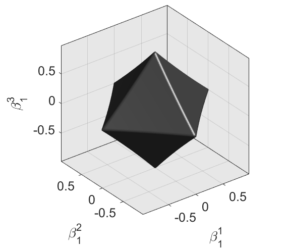
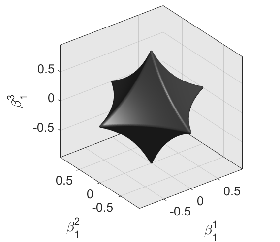
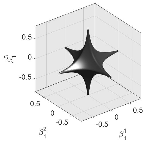
In Figure 1 we show level surfaces of the full penalty term for , , , and different values of . Hence the surfaces plotted are the solutions of
We see that when is small, the surface is similar to the three-dimensional ball. For larger values of the surface becomes highly non-convex, with peaks aligned with the axes, where there is only one model that is non-null.
Let us now draw attention to the following facts.
- 1.
if and only if for all . That is, the variables used in groups and are distinct.
- 2.
Let be a solution of (2) with and some . Then each of the columns of is a solution of the Elastic Net optimization problem with penalty parameter . This follows immediately from the fact the if , the objective function in (2) decouples across the different groups, so that each term can be minimized separately.
- 3.
As we have that for all . That is, active variables in different groups are distinct.
In general, the argument in point 2 above shows that by appropriately choosing the penalty function , our method generalizes penalized regression estimators, such as the lasso (Tibshirani 1996), the elastic net (Zou and Hastie 2005) and the SCAD (Fan and Li 2001), allowing for the selection of possibly overlapping subsets of features in such a way that variables that work well together end up in the same model, while at the same time encouraging diversity between the models, to reduce the correlation between the predictions resulting from each of them. This implies that, by appropriately choosing the tuning parameters the proposed method automatically and optimally decides: which variables are left out, the distribution of the active variables among the different models (with possible overlap) and the amount of shrinkage applied to the active variables in each of the models.
Once we have obtained the estimates by minimizing (2) we must aggregate them to form an overall fit or prediction by averaging these models: if is a training point (new observation), the fitted value (prediction) is given by
| (5) |
Since the output of our method consists of fitted models to be used together for model fitting and/or prediction, we can view our method as a way of optimal selection of models for ensembling. Therefore, there is a connection between our method and model ensembling, a powerful prediction tool. Examples of ensemble methods for regression include Random Forests (Breiman 2001) and Boosting (Schapire and Freund 2012; Friedman 2001). Both methods can adapt well to the presence of non-linearity, but the resulting prediction rules are generally difficult to interpret. If the relation between the response and the predictor variables is approximately linear, an ensemble of linear models produces highly competitive predictions and yield more interpretable results. The groups of variables into which the features are split are not predetermined and can overlap. The groups are in fact learned from the data through the optimization of the objective function. This is in sharp contrast with the approach in group lasso (Yuan and Lin 2006) where pre-existing domain knowledge determines the assignment of variables to groups.
The problem of minimizing (2) can be posed as an ‘artificial’ multivariate linear regression problem. Let be the matrix with the vector repeated times as columns.
where is the Frobenius norm, stands for taking the absolute value coordinate-wise and is the sum of the absolute values of the entries of the matrix. It is seen that the diversity penalty term in a sense penalizes correlations between the different models.
2.1 The case of orthogonal predictors
The objective function in (2) consists of three terms: a goodness of fit term (the least squares loss), a sparsity penalty term (the penalty), and the diversity penalty term introduced in this paper. By now the interplay between the least squares loss and the sparsity penalty is well understood. Our goal here is to shed some light on the role played by the diversity penalty in the solutions of (2). Unfortunately, the optimization problem that defines the SplitReg estimator does not in general have a closed form solution. However, closed form solutions can be derived for some very simple cases. In the following proposition we derive such closed form solution for the minimizers of the objective function when and the predictors are orthogonal. These simple results give a good indication of the effect that the diversity penalty has on the solutions of (2). Namely, Proposition 1 below will show that:
- 1.
If the maximal absolute correlation between the predictors and the response is below , then all the coefficients of the SplitReg solution are equal to zero.
- 2.
On the other hand if the maximal absolute correlation between the predictors and the response exceeds we have essentially two possible distinct regimes depending on the value of the diversity penalty constant .
- a)
When , diversity is not enforced and the features are active in both models.
- b)
When diversity is fully enforced and the features can be active in at most one of the two models.
- a)
Proposition 1.
Suppose that and is orthogonal. For let . Then
- 1.
If the -th coefficients in the two models for all solutions of SplitReg are zero.
- 2.
If
- (a)
If all solutions of SplitReg satisfy
where soft is the soft-thresholding operator, defined by .
- (b)
If any pair that satisfies and
is a solution to SplitReg.
- (c)
If all solutions of SplitReg satisfy that only one of and is zero, and the non-zero one is equal to
- (a)
2.2 The case of two correlated predictors
Further insights into how our procedure works can be gained by analyzing the simple case in which there are only two correlated predictors and two models.
Proposition 2.
Assume is normalized so that its columns have squared norm equal to and . Let be any solution of SplitReg, and , .
- 1.
If the models are disjoint then the active variables in each model have coefficients
and
- 2.
If variable is inactive in both models, variable is active in both models and then the coefficients of variable are equal to
- 3.
Assume and that both variables are active in both models. If and then all solutions of SplitReg satisfy
If , the solution is unique.
The case in which is easier to analyze. In this case, the proposition above implies that if the fitted models are disjoint then and the non-null coefficients of SplitReg are equal to the marginal Elastic Net regressions. Note that in the case in which , the size of the diversity penalty required to separate the models decreases as the correlation between the variables increases.
3 Computing SplitReg
We wish to compute that minimizes
with and
For any , as and hence a global minimum of exists. But the problem of finding the global minimum, , is not straightforward because is a non-convex function of , due to the non-convexity of . Still we are able to construct an efficient computing algorithm that converges to a coordinate-wise minimum. We first observe that the objective function is convex (strictly if ) in each coordinate, , and in each group of coordinates, , since the corresponding optimization problems are penalized least squares problems with a weighted elastic net penalty. In fact, for any fixed we have
where
Hence, for each group and for each coordinate separately we have an elastic net type problem, where the lasso penalty has weights which depend on the solution itself. In particular, the coordinates most penalized in model will be those that have large coefficients in the other models.
3.1 Computing solutions for fixed and
Based on the previous discussion, we propose a computing algorithm based on coordinate descent. Coordinate descent has proven to be efficient for solving regularized least squares problems, see Friedman et al. (2010) for example. The following result is the main building block of this algorithm.
Proposition 3.
The coordinate descent update for is given by
where is the in-sample prediction of using model and leaving out variable .
Note that the shrinkage being applied to the coefficient of variable in model , , increases with the sum of the absolute values of the coefficients of variable in all other models. This shows more clearly that the penalty encourages diversity among the models.
We cycle through the coordinates of , then through those of and so on until we reach , where we check for convergence. Convergence is declared when
for some small positive . Since the data is standardized, the convergence criterion in the original units is:
Hence, the algorithm converges when the in-sample average predictions no longer change significantly. The following Proposition follows immediately from Theorem 4.1 of Tseng (2001)
Proposition 4.
The proposed algorithm converges to a coordinate-wise minimizer of (2).
3.2 Choosing the penalty parameters
We choose and over grids of candidates, looking to minimize the cross-validated (CV) mean squared prediction error (MSPE). The grids of candidates are built as follows. Let be the smallest that makes all models null. Clearly depends on . It is easy to show that for and , . For we estimate by performing a grid search. For each , the corresponding is the maximum sparsity penalty that will be considered. The smallest that maximises diversity among the models (makes them disjoint) for a given , say , is also estimated using a grid search. To build a grid to search for the optimal we take 100 log-equispaced points between and , where is if and otherwise. The grid used for is built analogously, but including zero as a candidate.
Even though we could also cross-validate over a grid of possible values of , we find that taking a large value of , say or , generally works well and hence in what follows we assume that is fixed.
Fix one of , . We then minimize the objective function over the grid of candidates corresponding to the other penalty term, going from the largest to the smallest values in the grid; for each element of the grid of candidates, the solution to the problem using the previous element is used as a warm start. Even though the optimal is not in general a continuous function of and , see Proposition 1, we find that using warm starts as described above works well in practice.
The main loop of the algorithm works as follows, starting with , and until the CV MSPE no longer decreases:
- •
Find the in the grid giving minimal CV MSPE, .
- •
Take the optimal from the previous step. Recompute and the corresponding grid. Find the in the grid giving minimal cross-validated MSPE, . Go to the previous step.
As we mentioned earlier, since we start with , the solution with all columns equal to a elastic net estimator is always a candidate to be chosen.
3.3 The number of models
We conduct a small simulation study to illustrate the effect increasing the number of models has on the computation time and the performance of SplitReg-Lasso. We generate 100 replications of a linear model with predictors and observations, corresponding to the second covariance structure described in Section 5. For each replication, two data-sets are generated, one on which SplitReg is trained and one used for computing the mean squared prediction error (MSPE). The computation is repeated for various values of the proportion of active variables, called . The signal to noise ratio is 10. We show the MSPEs for different values of the number of models used (rows) and the proportion of active variables in the data generating process (columns). We also computed a measure of the overlap between the models of SplitReg. Let be the matrix with columns equal to the computed models, where is the number of models and the number of features. Let then we define the overlap as
if , and as 0 otherwise. Note that . If then all models are empty, whereas if , then at least one model is non-empty and actually . If then each variable that is active can only appear in one model, and hence the overlap between the models is minimal, since they are disjoint. Finally, if then all the variables that are active in at least one model, actually appear in all the models, and hence we have maximum overlap.
Table 1 shows the results. In all the considered cases, as the number of models increases, both the overlap and the MSPE decrease. The gains in prediction accuracy, however, decrease at and nearly cease passing . There seems to be a ‘diminishing returns’ type phenomenon.
The last column of Table 1 shows the average computation time in seconds. The computation time doesn’t vary much for the different sparsity levels. Hence we report the average over them. In all the settings studied in this paper, the increase in computational time due to using more models, appears to be approximately linear in the number of models, as evidenced by Table 1. From this table we see that the average computing time is approximately 3.19+3 seconds.
An objective way to determine a nearly optimal number of models to be used, is to cross-validate over a coarse grid, say, taking or models; this is the approach we take in Section 6, where we apply the proposed methodology to a real data-set. In our simulations we always use ten models, a possibly sub-optimal choice, but still good enough to give an excellent performance.
| MSPE | OVP | MSPE | OVP | MSPE | OVP | Time | |
|---|---|---|---|---|---|---|---|
| 2 | 1.27 | 0.64 | 1.23 | 0.66 | 1.23 | 0.63 | 8.61 |
| 5 | 1.22 | 0.44 | 1.18 | 0.43 | 1.17 | 0.37 | 19.25 |
| 7 | 1.22 | 0.42 | 1.17 | 0.38 | 1.17 | 0.36 | 25.23 |
| 10 | 1.21 | 0.38 | 1.16 | 0.36 | 1.16 | 0.33 | 33.97 |
| 15 | 1.19 | 0.35 | 1.15 | 0.36 | 1.15 | 0.32 | 48.98 |
| 20 | 1.20 | 0.35 | 1.15 | 0.34 | 1.15 | 0.30 | 64.05 |
| 30 | 1.19 | 0.31 | 1.15 | 0.33 | 1.15 | 0.29 | 95.69 |
4 A consistency result
Assume the data follows a standard linear regression model
| (6) |
where the vector of predictors is fixed and the errors are i.i.d. normal random variables with variance . The number of predictors may depend on the sample size and be greater than . As before, we assume that for .
Theorem 1.
Let . Assume that for some . Let be any solution of (2). Then with probability at least we have
It follows that if we take to be of order and to be of order then if we assume and are of order smaller than and , the average prediction, , is consistent. A similar result can be obtained if one assumes only that the errors have a sub-gaussian distribution. Sharper bounds may be obtained if one assumes more restrictive conditions on the set of predictor variables, for example the so-called compatibility condition; see Section 6.2.2 of Bühlmann and van de Geer (2011) for details. An overview of consistency results for regularized estimators is available in, for example, Bühlmann and van de Geer (2011). In the more classical case in which the smallest eigenvalue of is bounded below by a fixed constant, for example when is taken to be fixed and converges to a positive definite matrix, we may deduce that in probability as goes to infinity.
5 Simulations
5.1 Methods
An R package that implements the procedures proposed in this paper, called SplitReg is available from CRAN. We ran a simulation study, comparing the prediction accuracy of the following eleven competitors. All computations were carried out in R.
- 1.
Lasso, computed using the glmnet package.
- 2.
Elastic net with , computed using the glmnet package.
- 3.
Split regularized regression using and lasso sparsity penalty, called SplitReg-Lasso.
- 4.
Split regularized regression using and elastic net sparsity penalty, called SplitReg-EN.
- 5.
Sure independence screening (SIS) procedure, Fan and Lv (2008), followed by fitting a SCAD penalized least squares estimator, computed using the SIS package, called SIS-SCAD.
- 6.
MC+ penalized least squares estimator, Zhang (2010), computed using the sparsenet package, called SparseNet.
- 7.
Relaxed Lasso, Meinshausen (2007), computed using the relaxnet package, called Relaxed.
- 8.
Forward stepwise algorithm, computed using the lars package, called Stepwise.
- 9.
Cluster representative lasso, proposed in Bühlmann et al. (2013), computed using code kindly provided by the authors, called CRL.
- 10.
Random forest of Breiman (2001), computed using the randomForest package, called RF.
- 11.
Random GLM method of Song et al. (2013), computed using the randomGLM package, called RGLM.
All tuning parameters were chosen via cross-validation; the RF and RGLM methods were ran using their default settings. The CRL of Bühlmann et al. (2013) was not included in scenarios with due to its long computation time when compared with the rest of the methods. For the same reason, in the scenarios with , we only did 100 replications for CRL, instead of the 300 done for all the other procedures.
The popular group lasso Yuan and Lin (2006); Simon et al. (2013) is not included in the simulation, because we don’t assume that there is a priori knowledge of the existence of pre-defined groups among the features. The interesting recent proposals of Bühlmann et al. (2013), Sharma et al. (2013) and Witten et al. (2014), assume that there exist unknown clusters of correlated variables, and shrink the coefficients of variables in the same cluster towards each other. Because CRL has a relatively more efficient numerical implementation (compared with the other two) we included it in our simulation to represent the cluster-based approaches. Finally, note that all the competitors above, except perhaps for the forward stepwise algorithm, the RF and the RGLM, could in principle be used as building blocks in our procedure. One of the main objectives of this simulation study is to show that the proposed method for splitting the features improves upon the prediction accuracy of the base estimators being pooled together, in this case, the Lasso and the Elastic Net.
5.2 Models
For each Monte Carlo replication, we generate data from a linear model:
where the are multivariate normal with zero mean and correlation matrix and the are standard normal. We consider two combinations of and , namely and . For each , we take the number of active variables to be with and .
For all scenarios, the nonzero elements of the -dimensional vectors are randomly generated as described in Fan and Lv (2008). We set , and set nonzero coefficients to be for each model, where was drawn from a Bernoulli distribution with parameter 0.2 and is drawn from the standard Gaussian distribution. For , the -norms range from 18.50 to 54.80 for all sparsity levels considered. For , the -norms range from 7.94 to 21.13.
Given , and a sparsity level , the following scenarios for and are considered
-
Scenario 1 for all , the first coordinates of are nonzero and the rest are equal to zero.
-
Scenario 2
for , for and the rest of the coordinates equal to zero.
-
Scenario 3
the first coordinates of are nonzero and the rest are zero.
We consider different values of : , , . Then is chosen to give a desired signal to noise ratio (SNR), defined as We consider SNRs of 3, 5 and 10. In Scenario 1, all the predictors are correlated among each other. In Scenario 2, we have two groups of active variables, similar to the simulation scenario considered in Witten et al. (2014). Variables within each group are correlated with each other, but the groups are independent. In Scenario 3, the active variables are only correlated with each other. We report results for all scenarios across all considered correlations, SNRs and the two combinations of and .
5.3 Performance measures
For each replication, two independent copies of the data are generated, one to fit the procedures, the other one to compute the MSPE, divided by the variance of the noise, . Hence, the best possible result is . In each table reporting the MSPEs, we also compute the standard error for each of the methods, and report the maximum among them in the caption. We also compute and report the precision (PR) and recall (RC) of each method, defined as
Note that large values of PR and RC are desirable. For SplitReg, the vector of coefficients used to compute the precision and recall is the average of the models, see (5). For the SIS-SCAD method, the precision and recall are computed using the variables selected by the SIS step. For the RGLM method, the precision and recall are computed using the union of the variables selected in each of the bags. Since RF does not fit a linear model, we do not compute its precision and recall.
5.4 Results
In Table 2 we report the average rank for all the compared methods with the exception of CRL because this method was only evaluated in the case . Rank 1 corresponds to the top performer method and rank 10 corresponds to the worst performing method. The average ranks are evaluated across all the considered scenarios, correlations, SNRs and sparsity levels. We report the average ranks for each of the two considered combinations of and , and the overall average ranks. The average ranks of the best two performing methods are displayed in bold face.
For , SplitReg-EN and SplitReg-Lasso have the best average ranks for the MSPE, with RGLM being the runner up. We also note that the average recall ranks of SplitReg-Lasso and SplitReg-EN are better than those of the corresponding base estimators Lasso and elastic net, respectively, and also better than the other competitors, except for RGLM. The price paid by RGLM for this improvement is a severe decrease in precision, as RGLM has the worst average rank regarding precision.
For , SplitReg-EN and SplitReg-Lasso again have the best average MSPE ranks. However, RGLM is no longer the closest competitor as it now displays the worst average MSPE rank. RGLM also has the worst average rank for the precision, indicating that too many noise variables were selected by the algorithm, deteriorating its performance. The average rank for the recall of SplitReg-Lasso and SplitReg-EN is again better than that of the base estimators Lasso and elastic net.
Regarding the overall average ranks, SplitReg-EN and SplitReg-Lasso have the best MSPE performance, RGLM is the clear winner regarding recall rank. But this improvement of RGLM in terms of recall rank is at the cost of an important loss in precision, particularly in the case of . The relaxed Lasso and forward stepwise regression typically have the best overall precision ranks, but the methods are not competitive regarding MSPE and recall.
In the scenarios we consider, Elastic Net and Lasso behave very similarly, as do SplitReg-EN and SplitReg-Lasso. This is somewhat surprising specially in cases where the correlation among the variables is high, since this is where the elastic net penalty would be expected to perform better than -regularization.
| Overall Rank | |||||||||
| Method | MSPE | RC | PR | MSPE | RC | PR | MSPE | RC | PR |
| Lasso | 5.11 | 5.80 | 4.53 | 2.86 | 3.19 | 3.35 | 3.99 | 4.50 | 3.94 |
| Elastic Net | 3.93 | 4.56 | 4.30 | 2.68 | 2.79 | 3.70 | 3.31 | 3.67 | 4.00 |
| SplitReg-Lasso | 2.09 | 2.82 | 6.73 | 1.67 | 1.93 | 4.17 | 1.88 | 2.38 | 5.45 |
| SplitReg-EN | 1.59 | 2.18 | 6.61 | 1.93 | 1.83 | 4.43 | 1.76 | 2.00 | 5.52 |
| SparseNet | 6.03 | 4.70 | 3.04 | 3.14 | 3.81 | 2.53 | 4.58 | 4.25 | 2.79 |
| Relaxed | 6.60 | 7.09 | 2.39 | 3.28 | 4.92 | 1.49 | 4.94 | 6.00 | 1.94 |
| Stepwise | 9.51 | 9.00 | 3.37 | 5.00 | 5.89 | 1.27 | 7.25 | 7.45 | 2.32 |
| RF | 7.49 | 4.76 | 6.12 | ||||||
| RGLM | 3.45 | 1.00 | 8.35 | 6.47 | 1.00 | 6.00 | 4.96 | 1.00 | 7.17 |
| SIS-SCAD | 9.19 | 7.84 | 5.69 | 4.89 | 4.75 | 3.06 | 7.04 | 6.29 | 4.38 |
6 Glass data-sets
We analyze the performance of the competitors considered in the previous section when predicting on real data-sets from a chemometric problem. To evaluate the prediction accuracy of the competitors we randomly split the data into a training set that has of the observations and a testing set that has the remaining . This is repeated 100 times and the resulting MSPEs are averaged. The results are reported relative to the best average performance among all estimators. Hence, the estimator with the best average performance will have a score of 1. We also report the average rank among the data-sets for each method.
The glass data-sets Lemberge et al. (2000) were obtained from an electron probe X-ray microanalysis (EPXMA) of archaeological glass samples. A spectrum on 1920 frequencies was measured on a total of 180 glass samples. The goal is to predict the concentrations of the following chemical compounds using the spectrum: Na2O, MgO, Al2O3, SiO2, P2O5, SO3, Cl, K2O, CaO, MnO, Fe2O3, BaO and PbO. After removing predictors with little variation, we are left with frequencies and observations. The CRL estimator was not included in the comparison, due to its long computation time. The number of models used to form the ensembles is chosen by cross-validation among the values 2, 5, 7, 10. The elastic net and SplitReg-EN were computed with , closer to a Ridge than a Lasso estimator, since we a priori expected a relatively low level of sparsity.
Table 3 shows the results. Highlighted in black is the best performing method for each compound. It is seen that SplitReg-Lasso has the best overall behavior, having the highest average rank (1.92) over the thirteen compounds. Excluding SplitReg-EN which performs similarly to SplitReg-Lasso, the RGLM is the strongest competitor, with a rank of 3.54.
| Method | Na2O | MgO | Al2O3 | SiO2 | P2O5 | SO3 | Cl | K2O | CaO | MnO | Fe2O3 | BaO | PbO | Rank |
|---|---|---|---|---|---|---|---|---|---|---|---|---|---|---|
| Lasso | 1.70 | 1.16 | 1.38 | 2.78 | 1.19 | 1.14 | 1.39 | 1.41 | 1.48 | 1.09 | 1.38 | 1.04 | 1.01 | 4.23 |
| Elastic Net | 1.62 | 1.18 | 1.74 | 2.73 | 1.31 | 1.17 | 1.13 | 1.44 | 1.47 | 1.05 | 1.23 | 1.01 | 1.08 | 4.62 |
| SplitReg-Lasso | 1.31 | 1.00 | 1.00 | 1.67 | 1.00 | 1.00 | 1.00 | 1.36 | 1.40 | 1.05 | 1.26 | 1.03 | 1.00 | 1.92 |
| SplitReg-EN | 1.58 | 1.18 | 1.66 | 2.56 | 1.25 | 1.12 | 1.10 | 1.43 | 1.47 | 1.04 | 1.20 | 1.00 | 1.08 | 3.38 |
| SparseNet | 1.63 | 1.31 | 1.76 | 2.84 | 1.28 | 1.18 | 1.54 | 1.53 | 1.57 | 1.15 | 1.42 | 1.06 | 1.06 | 6.31 |
| Relaxed | 1.80 | 1.23 | 1.40 | 2.81 | 1.16 | 1.19 | 1.38 | 1.40 | 1.49 | 1.13 | 1.46 | 1.10 | 1.28 | 5.62 |
| Stepwise | 2.40 | 2.13 | 3.72 | 4.10 | 2.65 | 1.52 | 4.75 | 1.89 | 1.78 | 1.18 | 1.51 | 2.32 | 1.73 | 9.00 |
| RF | 1.00 | 1.95 | 7.04 | 3.02 | 16.48 | 1.16 | 12.06 | 6.93 | 9.18 | 1.16 | 1.00 | 2.69 | 6.34 | 7.77 |
| RGLM | 1.80 | 1.02 | 1.20 | 1.00 | 1.00 | 1.26 | 1.62 | 1.00 | 1.00 | 1.00 | 1.19 | 1.72 | 1.04 | 3.54 |
| SIS-SCAD | 2.01 | 4.19 | 1.70 | 2.88 | 1.85 | 1.29 | 1.87 | 2.08 | 2.08 | 1.19 | 1.67 | 1.68 | 1.95 | 8.62 |
7 Discussion
We have proposed a novel method for splitting variables in linear regression models. The seminal work by Breiman (2001) points out that the performance of a given ensemble of models depends on the strength of the models and their diversity. We believe that the good performance of SplitReg derives from the fact that the loss function underlying this procedure encourages a good balance between the models strength and their diversity. In the limiting case when the penalty parameters for the diversity penalty, , is equal to zero, all the columns of the matrix are identical and equal to the elastic net solution. In the opposite limiting case there is at most one non-zero element on each row of the matrix In practice, the value of is chosen by cross-validation and the result is a compromise between these two extremes. Another factor that may influence the performance of a given ensemble is the weight assigned to each model. This is not optimized by SplitReg where all the models are given equal weight. On the other hand, the paper by Ando and Li (2014) do not optimize the generation of the models, putting the accent on the assignment of the weights. Therefore, their work and ours are complementary.
Examples using real and synthetic data-sets show that the approach systematically improves the prediction accuracy of the base estimators being pooled together. In the synthetic data-sets, the improvements tend to increase with the signal to noise ratio and the number of active variables. For low values of the signal to noise ratio, or when the number of active variables is small, the improvements are negligible. We believe that the results reported in this paper show that the proposed method is a valuable addition to the practitioners toolbox.
The approach taken in this paper can be extended in several ways. Other sparsity penalties such as the SCAD can be handled similarly. In fact, the algorithm proposed here will work with any regularized model approach provided the coordinate descent updates can be expressed in closed form. Our method can be extended to GLMs by splitting variables for GLM estimators instead of linear regression estimators. For example, groups of logistic regression models can be formed by replacing the quadratic loss in (2) with the deviance. The method can be robustified to deal with outliers by using, for example, a bounded loss function to measure the goodness of fit of each model in (2), instead of the classical least squares loss; in this case regularized robust regression estimators (see Smucler and Yohai (2017) for example) would be formed. Lower computational times may be achieved by using early stopping strategies when computing solution paths over one of the penalties and also by using an active set strategy when cycling over the groups, see Friedman et al. (2010).
Acknowledgments
Part of this work was conducted while Ezequiel Smucler was a postdoctoral research fellow at the departments of Statistics and of Computer Science at The University of British Columbia.
SUPPLEMENTARY MATERIAL
The supplemental material available contains the proofs of all results stated in the paper and the full results of our simulation study. An R package that implements the procedures proposed in this paper, called SplitReg is available from CRAN.
References
- Ando and Li (2014) Ando, T. and Li, K.-C. (2014). A model-averaging approach for high-dimensional regression. Journal of the American Statistical Association, 109(505):254–265.
- Breiman (1995) Breiman, L. (1995). Better subset regression using the nonnegative garrote. Technometrics, 37(4):373–384.
- Breiman (2001) Breiman, L. (2001). Random forests. Machine Learning, 45(1):5–32.
- Bühlmann et al. (2013) Bühlmann, P., Rütimann, P., van de Geer, S., and Zhang, C.-H. (2013). Correlated variables in regression: Clustering and sparse estimation. J. Statist. Planng Inf., 143(11):1835 – 1858.
- Bühlmann and van de Geer (2011) Bühlmann, P. and van de Geer, S. (2011). Statistics for High-Dimensional Data: Methods, Theory and Applications. Springer Series in Statistics. Springer Berlin Heidelberg.
- Christidis et al. (2018) Christidis, A., Aelst, S. V., and Zamar, R. (2018). Split regression modeling. arXiv:1812.05678.
- Fan and Li (2001) Fan, J. and Li, R. (2001). Variable selection via nonconcave penalized likelihood and its oracle properties. J. Am. Statist. Ass., 96(456):1348–1360.
- Fan and Lv (2008) Fan, J. and Lv, J. (2008). Sure independence screening for ultrahigh dimensional feature space. J. R. Statist. Soc. B, 70(5):849–911.
- Friedman (2001) Friedman, J. H. (2001). Greedy function approximation: A gradient boosting machine. Ann. Statist., 29(5):1189–1232.
- Friedman et al. (2010) Friedman, J. H., Hastie, T., and Tibshirani, R. (2010). Regularization paths for generalized linear models via coordinate descent. Journal of Statistical Software, 33(1):1.
- Hoerl and Kennard (1970) Hoerl, A. E. and Kennard, R. W. (1970). Ridge regression: Biased estimation for nonorthogonal problems. Technometrics, 12(1):55–67.
- Lemberge et al. (2000) Lemberge, P., De Raedt, I., Janssens, K. H., Wei, F., and Van Espen, P. J. (2000). Quantitative analysis of 16-17th century archaeological glass vessels using pls regression of epxma and -xrf data. Journal of Chemometrics, 14(5-6):751–763.
- Meinshausen (2007) Meinshausen, N. (2007). Relaxed lasso. Computational Statistics & Data Analysis, 52(1):374–393.
- Schapire and Freund (2012) Schapire, R. E. and Freund, Y. (2012). Boosting: Foundations and Algorithms. The MIT Press.
- Sharma et al. (2013) Sharma, D. B., Bondell, H. D., and Zhang, H. H. (2013). Consistent group identification and variable selection in regression with correlated predictors. Journal of Computational and Graphical Statistics, 22(2):319–340.
- Simon et al. (2013) Simon, N., Friedman, J., Hastie, T., and Tibshirani, R. (2013). A sparse-group lasso. Journal of Computational and Graphical Statistics, 22(2):231–245.
- Smucler and Yohai (2017) Smucler, E. and Yohai, V. J. (2017). Robust and sparse estimators for linear regression models. Computational Statistics & Data Analysis, 111(C):116–130.
- Song et al. (2013) Song, L., Langfelder, P., and Horvath, S. (2013). Random generalized linear model: a highly accurate and interpretable ensemble predictor. BMC bioinformatics, 14(1):5.
- Tibshirani (1996) Tibshirani, R. (1996). Regression shrinkage and selection via the lasso. J. R. Statist. Soc. B, 58(1):267–288.
- Tseng (2001) Tseng, P. (2001). Convergence of a block coordinate descent method for nondifferentiable minimization. J. Optim. Theory Appl., 109(3):475–494.
- Witten et al. (2014) Witten, D., Shojaie, A., and Zhang, F. (2014). The cluster elastic net for high-dimensional regression with unknown variable grouping. Technometrics, 56(1):112–122.
- Yuan and Lin (2006) Yuan, M. and Lin, Y. (2006). Model selection and estimation in regression with grouped variables. J. R. Statist. Soc. B, 68(1):49–67.
- Zhang (2010) Zhang, C.-H. (2010). Nearly unbiased variable selection under minimax concave penalty. Ann. Statist., 38(2):894–942.
- Zou and Hastie (2005) Zou, H. and Hastie, T. (2005). Regularization and variable selection via the elastic net. J. R. Statist. Soc. B, 67(2):301–320.
Appendix A: Proofs of the results in the main paper
Proof of Proposition 1.
Consider any solution of SplitReg, , and fix . Let . The orthogonality of implies that
Hence if , . This proves 1.
Assume now and until the end of this proof that . Moreover, assume for now that . The case is dealt with similarly. Since , it can’t happen that . Assume that only one of or holds. Without loss of generality, we can assume . Hence
so that it must be that and hence that which implies . We have thus shown that if , and are both non-zero. Now assume both and are non-zero and . Then
Solving for gives 2(a) for , the same argument proves it for .
Using the orthogonality of it is easy to show that for any
In particular, if as before is any solution to SplitReg, we have that for all and hence minimizes
If , we get
Assume is the non-null coordinate of SplitReg. If we have
which is minimized whenever ; if the corresponding expression is minimized whenever . This proves 2(b).
Now take . Assume that there exists a solution of SplitReg such that for , , both and are non-zero, whereas for , at most one of and is non-zero. Take equal to except that for , coordinate is equal to and coordinate is equal to zero. Note that
Hence, the definition of implies that
Straightforward calculations show that
By definition of , , and hence since , , a contradiction. Thus if , only one of and is zero and the non-zero one has to be equal to
which proves 2(c). ∎
Proof of Proposition 2.
Let . We first prove 1. We assume that , the other case is similar. Then it is easy to show that
Since
it must be that
from which the result follows immediately.
To prove 2, assume , the other case is proven similarly. Then
Proceeding as in the proof of Proposition 1, the result follows.
Now we prove 3. It is easy to show that
Hence
and
The eigenvalues of the matrix on the left hand side are . Hence if the linear system has a unique solution. ∎
Proof of Theorem 1.
Let for the matrix in with columns equal to . Let . Let be the matrix with columns equal to . Then the linear model can be written as
Let
and
Let be any solution to SplitReg. Then
Hence
where is the coordinate-wise maximum absolute value and is the sum of the absolute values. It follows that
Since is standard normal
Thus with probability at least
Since , we have
Hence
| (7) |
∎
Appendix B: Full results of the simulation study
The maximum standard error reported in the caption of each table does not include cases where the average prediction mean squared errors was greater than 3.
| Method | MSPE | RC | PR | MSPE | RC | PR | MSPE | RC | PR | MSPE | RC | PR |
|---|---|---|---|---|---|---|---|---|---|---|---|---|
| Lasso | 1.74 | 0.15 | 0.13 | 1.59 | 0.10 | 0.16 | 1.46 | 0.08 | 0.25 | 1.44 | 0.07 | 0.44 |
| Elastic Net | 1.72 | 0.16 | 0.13 | 1.57 | 0.11 | 0.16 | 1.45 | 0.08 | 0.25 | 1.41 | 0.08 | 0.43 |
| SplitReg-Lasso | 1.58 | 0.41 | 0.09 | 1.38 | 0.37 | 0.14 | 1.28 | 0.34 | 0.23 | 1.22 | 0.32 | 0.42 |
| SplitReg-EN | 1.56 | 0.42 | 0.10 | 1.38 | 0.37 | 0.14 | 1.27 | 0.36 | 0.23 | 1.21 | 0.35 | 0.42 |
| SparseNet | 1.76 | 0.16 | 0.14 | 1.63 | 0.11 | 0.17 | 1.50 | 0.09 | 0.26 | 1.46 | 0.08 | 0.45 |
| Relaxed | 1.80 | 0.12 | 0.15 | 1.66 | 0.07 | 0.17 | 1.54 | 0.06 | 0.25 | 1.51 | 0.06 | 0.44 |
| Stepwise | 2.83 | 0.02 | 0.15 | 2.59 | 0.01 | 0.18 | 2.46 | 0.01 | 0.26 | 2.41 | 0.01 | 0.44 |
| RF | 1.94 | 1.82 | 1.77 | 1.72 | ||||||||
| RGLM | 1.50 | 0.77 | 0.06 | 1.32 | 0.74 | 0.11 | 1.23 | 0.71 | 0.21 | 1.17 | 0.70 | 0.40 |
| SIS-SCAD | 2.65 | 0.05 | 0.13 | 2.41 | 0.03 | 0.15 | 2.24 | 0.03 | 0.24 | 2.17 | 0.02 | 0.43 |
| Method | MSPE | RC | PR | MSPE | RC | PR | MSPE | RC | PR | MSPE | RC | PR |
|---|---|---|---|---|---|---|---|---|---|---|---|---|
| Lasso | 2.09 | 0.19 | 0.15 | 1.85 | 0.13 | 0.18 | 1.66 | 0.10 | 0.26 | 1.59 | 0.09 | 0.44 |
| Elastic Net | 2.07 | 0.20 | 0.15 | 1.84 | 0.13 | 0.18 | 1.64 | 0.10 | 0.26 | 1.56 | 0.09 | 0.44 |
| SplitReg-Lasso | 1.87 | 0.49 | 0.10 | 1.56 | 0.45 | 0.14 | 1.37 | 0.44 | 0.23 | 1.27 | 0.42 | 0.42 |
| SplitReg-EN | 1.85 | 0.48 | 0.10 | 1.55 | 0.45 | 0.14 | 1.37 | 0.44 | 0.23 | 1.27 | 0.44 | 0.42 |
| SparseNet | 2.11 | 0.20 | 0.16 | 1.89 | 0.14 | 0.19 | 1.67 | 0.12 | 0.28 | 1.59 | 0.10 | 0.47 |
| Relaxed | 2.19 | 0.16 | 0.16 | 1.96 | 0.10 | 0.18 | 1.74 | 0.08 | 0.27 | 1.66 | 0.07 | 0.45 |
| Stepwise | 0.03 | 0.17 | 0.02 | 0.18 | 0.01 | 0.26 | 2.94 | 0.01 | 0.44 | |||
| RF | 2.64 | 2.46 | 2.36 | 2.29 | ||||||||
| RGLM | 1.80 | 0.78 | 0.06 | 1.54 | 0.75 | 0.11 | 1.39 | 0.72 | 0.21 | 1.31 | 0.71 | 0.40 |
| SIS-SCAD | 0.06 | 0.15 | 2.81 | 0.03 | 0.17 | 2.57 | 0.03 | 0.25 | 2.45 | 0.02 | 0.44 | |
| Method | MSPE | RC | PR | MSPE | RC | PR | MSPE | RC | PR | MSPE | RC | PR |
|---|---|---|---|---|---|---|---|---|---|---|---|---|
| Lasso | 2.91 | 0.26 | 0.17 | 2.47 | 0.16 | 0.20 | 2.09 | 0.12 | 0.27 | 1.94 | 0.11 | 0.46 |
| Elastic Net | 2.88 | 0.26 | 0.17 | 2.43 | 0.17 | 0.19 | 2.07 | 0.13 | 0.27 | 1.90 | 0.11 | 0.45 |
| SplitReg-Lasso | 2.56 | 0.57 | 0.11 | 1.96 | 0.57 | 0.14 | 1.60 | 0.57 | 0.23 | 1.40 | 0.58 | 0.42 |
| SplitReg-EN | 2.56 | 0.56 | 0.11 | 1.98 | 0.56 | 0.14 | 1.60 | 0.57 | 0.23 | 1.40 | 0.58 | 0.42 |
| SparseNet | 2.88 | 0.29 | 0.18 | 2.45 | 0.19 | 0.21 | 2.06 | 0.15 | 0.29 | 1.89 | 0.13 | 0.49 |
| Relaxed | 0.21 | 0.18 | 2.60 | 0.13 | 0.20 | 2.17 | 0.10 | 0.27 | 2.00 | 0.09 | 0.46 | |
| Stepwise | 0.04 | 0.18 | 0.03 | 0.19 | 0.02 | 0.26 | 0.02 | 0.45 | ||||
| RF | ||||||||||||
| RGLM | 2.60 | 0.79 | 0.06 | 2.14 | 0.76 | 0.11 | 1.85 | 0.73 | 0.21 | 1.69 | 0.72 | 0.40 |
| SIS-SCAD | 0.08 | 0.18 | 0.04 | 0.19 | 0.03 | 0.26 | 0.02 | 0.44 | ||||
| Method | MSPE | RC | PR | MSPE | RC | PR | MSPE | RC | PR | MSPE | RC | PR |
|---|---|---|---|---|---|---|---|---|---|---|---|---|
| Lasso | 1.31 | 0.08 | 0.10 | 1.25 | 0.06 | 0.14 | 1.21 | 0.05 | 0.22 | 1.21 | 0.05 | 0.43 |
| Elastic Net | 1.30 | 0.08 | 0.10 | 1.23 | 0.06 | 0.14 | 1.21 | 0.05 | 0.22 | 1.20 | 0.05 | 0.43 |
| SplitReg-Lasso | 1.22 | 0.25 | 0.08 | 1.15 | 0.22 | 0.13 | 1.13 | 0.19 | 0.22 | 1.12 | 0.19 | 0.42 |
| SplitReg-EN | 1.22 | 0.25 | 0.08 | 1.15 | 0.22 | 0.12 | 1.14 | 0.20 | 0.22 | 1.11 | 0.20 | 0.42 |
| SparseNet | 1.35 | 0.08 | 0.11 | 1.28 | 0.06 | 0.15 | 1.24 | 0.05 | 0.24 | 1.24 | 0.04 | 0.45 |
| Relaxed | 1.37 | 0.06 | 0.10 | 1.31 | 0.04 | 0.14 | 1.26 | 0.04 | 0.23 | 1.26 | 0.03 | 0.43 |
| Stepwise | 1.84 | 0.01 | 0.11 | 1.77 | 0.01 | 0.16 | 1.72 | 0.01 | 0.22 | 1.69 | 0.01 | 0.43 |
| RF | 1.30 | 1.23 | 1.22 | 1.20 | ||||||||
| RGLM | 1.22 | 0.73 | 0.05 | 1.15 | 0.70 | 0.10 | 1.13 | 0.69 | 0.20 | 1.11 | 0.68 | 0.40 |
| SIS-SCAD | 2.23 | 0.03 | 0.08 | 2.12 | 0.02 | 0.11 | 2.03 | 0.02 | 0.21 | 2.06 | 0.02 | 0.40 |
| Method | MSPE | RC | PR | MSPE | RC | PR | MSPE | RC | PR | MSPE | RC | PR |
|---|---|---|---|---|---|---|---|---|---|---|---|---|
| Lasso | 1.43 | 0.10 | 0.11 | 1.34 | 0.07 | 0.15 | 1.28 | 0.06 | 0.23 | 1.27 | 0.06 | 0.43 |
| Elastic Net | 1.42 | 0.11 | 0.11 | 1.32 | 0.08 | 0.15 | 1.28 | 0.06 | 0.23 | 1.25 | 0.06 | 0.43 |
| SplitReg-Lasso | 1.31 | 0.31 | 0.09 | 1.20 | 0.28 | 0.13 | 1.17 | 0.24 | 0.22 | 1.14 | 0.24 | 0.42 |
| SplitReg-EN | 1.31 | 0.32 | 0.08 | 1.20 | 0.28 | 0.13 | 1.16 | 0.26 | 0.22 | 1.13 | 0.25 | 0.42 |
| SparseNet | 1.46 | 0.11 | 0.13 | 1.37 | 0.08 | 0.17 | 1.31 | 0.07 | 0.26 | 1.29 | 0.06 | 0.46 |
| Relaxed | 1.48 | 0.08 | 0.11 | 1.42 | 0.05 | 0.15 | 1.34 | 0.04 | 0.24 | 1.33 | 0.04 | 0.43 |
| Stepwise | 2.15 | 0.02 | 0.13 | 2.03 | 0.01 | 0.16 | 1.95 | 0.01 | 0.23 | 1.90 | 0.01 | 0.42 |
| RF | 1.52 | 1.43 | 1.41 | 1.37 | ||||||||
| RGLM | 1.29 | 0.75 | 0.05 | 1.18 | 0.72 | 0.11 | 1.14 | 0.70 | 0.20 | 1.11 | 0.69 | 0.40 |
| SIS-SCAD | 2.32 | 0.04 | 0.09 | 2.20 | 0.03 | 0.12 | 2.09 | 0.02 | 0.22 | 2.07 | 0.02 | 0.42 |
| Method | MSPE | RC | PR | MSPE | RC | PR | MSPE | RC | PR | MSPE | RC | PR |
|---|---|---|---|---|---|---|---|---|---|---|---|---|
| Lasso | 1.71 | 0.15 | 0.13 | 1.55 | 0.10 | 0.16 | 1.42 | 0.08 | 0.25 | 1.39 | 0.07 | 0.44 |
| Elastic Net | 1.69 | 0.16 | 0.13 | 1.53 | 0.10 | 0.16 | 1.41 | 0.08 | 0.25 | 1.37 | 0.07 | 0.43 |
| SplitReg-Lasso | 1.52 | 0.42 | 0.09 | 1.33 | 0.37 | 0.14 | 1.24 | 0.33 | 0.23 | 1.18 | 0.32 | 0.42 |
| SplitReg-EN | 1.52 | 0.42 | 0.09 | 1.33 | 0.38 | 0.14 | 1.23 | 0.34 | 0.23 | 1.18 | 0.33 | 0.42 |
| SparseNet | 1.73 | 0.17 | 0.15 | 1.54 | 0.12 | 0.19 | 1.43 | 0.10 | 0.28 | 1.40 | 0.08 | 0.48 |
| Relaxed | 1.77 | 0.12 | 0.14 | 1.62 | 0.08 | 0.16 | 1.49 | 0.06 | 0.25 | 1.45 | 0.05 | 0.44 |
| Stepwise | 2.81 | 0.02 | 0.14 | 2.56 | 0.01 | 0.16 | 2.39 | 0.01 | 0.26 | 2.32 | 0.01 | 0.42 |
| RF | 2.12 | 1.98 | 1.91 | 1.86 | ||||||||
| RGLM | 1.50 | 0.76 | 0.06 | 1.31 | 0.74 | 0.11 | 1.23 | 0.72 | 0.21 | 1.17 | 0.70 | 0.40 |
| SIS-SCAD | 2.74 | 0.05 | 0.11 | 2.48 | 0.03 | 0.14 | 2.29 | 0.02 | 0.24 | 2.28 | 0.02 | 0.42 |
| Method | MSPE | RC | PR | MSPE | RC | PR | MSPE | RC | PR | MSPE | RC | PR |
|---|---|---|---|---|---|---|---|---|---|---|---|---|
| Lasso | 1.14 | 0.04 | 0.07 | 1.11 | 0.03 | 0.12 | 1.12 | 0.03 | 0.21 | 1.11 | 0.03 | 0.41 |
| Elastic Net | 1.14 | 0.04 | 0.07 | 1.10 | 0.04 | 0.12 | 1.11 | 0.03 | 0.21 | 1.10 | 0.03 | 0.42 |
| SplitReg-Lasso | 1.10 | 0.14 | 0.07 | 1.07 | 0.12 | 0.12 | 1.08 | 0.11 | 0.21 | 1.07 | 0.11 | 0.41 |
| SplitReg-EN | 1.10 | 0.15 | 0.07 | 1.07 | 0.13 | 0.12 | 1.08 | 0.12 | 0.21 | 1.07 | 0.12 | 0.41 |
| SparseNet | 1.20 | 0.04 | 0.10 | 1.15 | 0.04 | 0.14 | 1.16 | 0.03 | 0.25 | 1.16 | 0.03 | 0.46 |
| Relaxed | 1.20 | 0.03 | 0.08 | 1.15 | 0.02 | 0.12 | 1.15 | 0.02 | 0.22 | 1.16 | 0.02 | 0.41 |
| Stepwise | 1.38 | 0.08 | 1.36 | 0.12 | 1.34 | 0.23 | 1.36 | 0.41 | ||||
| RF | 1.12 | 1.07 | 1.09 | 1.08 | ||||||||
| RGLM | 1.15 | 0.66 | 0.05 | 1.11 | 0.64 | 0.10 | 1.11 | 0.63 | 0.20 | 1.11 | 0.62 | 0.40 |
| SIS-SCAD | 2.05 | 0.02 | 0.06 | 2.02 | 0.02 | 0.11 | 1.98 | 0.02 | 0.20 | 1.97 | 0.02 | 0.40 |
| Method | MSPE | RC | PR | MSPE | RC | PR | MSPE | RC | PR | MSPE | RC | PR |
|---|---|---|---|---|---|---|---|---|---|---|---|---|
| Lasso | 1.18 | 0.05 | 0.08 | 1.14 | 0.04 | 0.12 | 1.14 | 0.04 | 0.22 | 1.13 | 0.03 | 0.41 |
| Elastic Net | 1.18 | 0.05 | 0.08 | 1.13 | 0.04 | 0.13 | 1.14 | 0.04 | 0.22 | 1.13 | 0.04 | 0.42 |
| SplitReg-Lasso | 1.13 | 0.18 | 0.07 | 1.08 | 0.16 | 0.12 | 1.09 | 0.15 | 0.22 | 1.08 | 0.14 | 0.42 |
| SplitReg-EN | 1.13 | 0.19 | 0.07 | 1.08 | 0.16 | 0.12 | 1.09 | 0.15 | 0.22 | 1.08 | 0.14 | 0.41 |
| SparseNet | 1.24 | 0.06 | 0.11 | 1.17 | 0.05 | 0.16 | 1.18 | 0.04 | 0.26 | 1.17 | 0.04 | 0.46 |
| Relaxed | 1.25 | 0.03 | 0.09 | 1.20 | 0.03 | 0.12 | 1.19 | 0.03 | 0.22 | 1.19 | 0.02 | 0.42 |
| Stepwise | 1.51 | 0.01 | 0.09 | 1.47 | 0.11 | 1.46 | 0.22 | 1.46 | 0.41 | |||
| RF | 1.17 | 1.11 | 1.13 | 1.12 | ||||||||
| RGLM | 1.17 | 0.69 | 0.05 | 1.12 | 0.67 | 0.10 | 1.12 | 0.66 | 0.20 | 1.11 | 0.65 | 0.40 |
| SIS-SCAD | 2.15 | 0.03 | 0.06 | 2.10 | 0.02 | 0.11 | 2.06 | 0.02 | 0.21 | 2.03 | 0.02 | 0.40 |
| Method | MSPE | RC | PR | MSPE | RC | PR | MSPE | RC | PR | MSPE | RC | PR |
|---|---|---|---|---|---|---|---|---|---|---|---|---|
| Lasso | 1.27 | 0.07 | 0.09 | 1.21 | 0.06 | 0.14 | 1.19 | 0.05 | 0.22 | 1.18 | 0.04 | 0.42 |
| Elastic Net | 1.26 | 0.08 | 0.09 | 1.20 | 0.06 | 0.14 | 1.18 | 0.05 | 0.22 | 1.17 | 0.05 | 0.43 |
| SplitReg-Lasso | 1.19 | 0.25 | 0.08 | 1.11 | 0.22 | 0.13 | 1.11 | 0.20 | 0.22 | 1.09 | 0.19 | 0.42 |
| SplitReg-EN | 1.19 | 0.25 | 0.08 | 1.11 | 0.23 | 0.13 | 1.11 | 0.20 | 0.22 | 1.09 | 0.19 | 0.42 |
| SparseNet | 1.31 | 0.09 | 0.12 | 1.23 | 0.07 | 0.18 | 1.22 | 0.06 | 0.28 | 1.22 | 0.05 | 0.48 |
| Relaxed | 1.33 | 0.05 | 0.10 | 1.27 | 0.04 | 0.14 | 1.23 | 0.03 | 0.23 | 1.24 | 0.03 | 0.42 |
| Stepwise | 1.74 | 0.01 | 0.11 | 1.70 | 0.01 | 0.14 | 1.65 | 0.01 | 0.22 | 1.60 | 0.01 | 0.41 |
| RF | 1.32 | 1.25 | 1.25 | 1.25 | ||||||||
| RGLM | 1.21 | 0.73 | 0.05 | 1.13 | 0.70 | 0.10 | 1.12 | 0.69 | 0.20 | 1.10 | 0.68 | 0.40 |
| SIS-SCAD | 2.25 | 0.03 | 0.07 | 2.14 | 0.02 | 0.11 | 2.08 | 0.02 | 0.21 | 2.05 | 0.02 | 0.40 |
| Method | MSPE | RC | PR | MSPE | RC | PR | MSPE | RC | PR | MSPE | RC | PR |
|---|---|---|---|---|---|---|---|---|---|---|---|---|
| Lasso | 1.79 | 0.98 | 0.26 | 2.01 | 0.63 | 0.34 | 1.98 | 0.42 | 0.39 | 1.72 | 0.31 | 0.52 |
| Elastic Net | 1.83 | 0.97 | 0.24 | 1.99 | 0.65 | 0.33 | 1.94 | 0.43 | 0.39 | 1.71 | 0.33 | 0.51 |
| SplitReg-Lasso | 1.78 | 0.98 | 0.27 | 1.99 | 0.69 | 0.30 | 1.85 | 0.62 | 0.32 | 1.55 | 0.68 | 0.46 |
| SplitReg-EN | 1.82 | 0.98 | 0.24 | 1.99 | 0.69 | 0.30 | 1.85 | 0.61 | 0.33 | 1.53 | 0.68 | 0.46 |
| SparseNet | 1.59 | 0.92 | 0.66 | 2.10 | 0.59 | 0.37 | 2.06 | 0.40 | 0.41 | 1.78 | 0.31 | 0.52 |
| Relaxed | 1.78 | 0.90 | 0.54 | 2.09 | 0.53 | 0.42 | 2.05 | 0.34 | 0.44 | 1.83 | 0.25 | 0.53 |
| Stepwise | 1.75 | 0.81 | 0.83 | 2.77 | 0.22 | 0.61 | 2.92 | 0.11 | 0.52 | 2.63 | 0.08 | 0.56 |
| RF | 2.40 | 2.15 | 1.94 | |||||||||
| RGLM | 1.00 | 0.05 | 2.79 | 0.98 | 0.10 | 0.99 | 0.20 | 0.99 | 0.40 | |||
| SIS-SCAD | 1.96 | 0.96 | 0.39 | 2.69 | 0.44 | 0.39 | 2.75 | 0.24 | 0.42 | 2.47 | 0.15 | 0.52 |
| CRL | 1.90 | 0.95 | 0.26 | 1.98 | 0.64 | 0.33 | 1.91 | 0.42 | 0.37 | 1.70 | 0.32 | 0.52 |
| Method | MSPE | RC | PR | MSPE | RC | PR | MSPE | RC | PR | MSPE | RC | PR |
|---|---|---|---|---|---|---|---|---|---|---|---|---|
| Lasso | 1.79 | 0.99 | 0.25 | 2.29 | 0.75 | 0.35 | 2.38 | 0.50 | 0.41 | 1.99 | 0.37 | 0.53 |
| Elastic Net | 1.86 | 1.00 | 0.23 | 2.28 | 0.76 | 0.34 | 2.35 | 0.51 | 0.41 | 1.97 | 0.38 | 0.53 |
| SplitReg-Lasso | 1.79 | 1.00 | 0.26 | 2.31 | 0.78 | 0.33 | 2.25 | 0.67 | 0.34 | 1.71 | 0.76 | 0.45 |
| SplitReg-EN | 1.85 | 1.00 | 0.23 | 2.31 | 0.78 | 0.32 | 2.24 | 0.66 | 0.34 | 1.70 | 0.76 | 0.45 |
| SparseNet | 1.37 | 0.98 | 0.78 | 2.44 | 0.71 | 0.38 | 2.48 | 0.50 | 0.42 | 2.05 | 0.37 | 0.54 |
| Relaxed | 1.64 | 0.97 | 0.60 | 2.35 | 0.66 | 0.44 | 2.49 | 0.41 | 0.46 | 2.09 | 0.30 | 0.55 |
| Stepwise | 1.43 | 0.96 | 0.88 | 0.30 | 0.64 | 0.15 | 0.56 | 0.10 | 0.57 | |||
| RF | 2.93 | 2.59 | ||||||||||
| RGLM | 1.00 | 0.05 | 0.98 | 0.10 | 0.98 | 0.20 | 2.59 | 0.99 | 0.40 | |||
| SIS-SCAD | 1.89 | 0.99 | 0.41 | 0.52 | 0.46 | 0.26 | 0.47 | 2.80 | 0.16 | 0.55 | ||
| CRL | 2.00 | 0.98 | 0.24 | 2.28 | 0.76 | 0.34 | 2.32 | 0.50 | 0.39 | 1.97 | 0.38 | 0.53 |
| Method | MSPE | RC | PR | MSPE | RC | PR | MSPE | RC | PR | MSPE | RC | PR |
| Lasso | 1.79 | 1.00 | 0.25 | 2.70 | 0.89 | 0.35 | 0.61 | 0.43 | 2.55 | 0.45 | 0.55 | |
| Elastic Net | 1.88 | 1.00 | 0.23 | 2.71 | 0.89 | 0.33 | 0.62 | 0.42 | 2.52 | 0.46 | 0.55 | |
| SplitReg-Lasso | 1.79 | 1.00 | 0.26 | 2.78 | 0.89 | 0.34 | 0.73 | 0.36 | 2.10 | 0.82 | 0.45 | |
| SplitReg-EN | 1.88 | 1.00 | 0.23 | 2.77 | 0.90 | 0.33 | 0.74 | 0.35 | 2.09 | 0.82 | 0.45 | |
| SparseNet | 1.23 | 1.00 | 0.87 | 2.75 | 0.87 | 0.39 | 0.62 | 0.43 | 2.61 | 0.46 | 0.56 | |
| Relaxed | 1.46 | 1.00 | 0.70 | 2.80 | 0.81 | 0.45 | 0.52 | 0.48 | 2.68 | 0.38 | 0.58 | |
| Stepwise | 1.26 | 1.00 | 0.92 | 0.49 | 0.65 | 0.20 | 0.57 | 0.13 | 0.59 | |||
| RF | ||||||||||||
| RGLM | 1.00 | 0.05 | 0.98 | 0.10 | 0.98 | 0.20 | 0.99 | 0.40 | ||||
| SIS-SCAD | 1.77 | 1.00 | 0.45 | 0.63 | 0.56 | 0.30 | 0.53 | 0.17 | 0.60 | |||
| CRL | 2.33 | 0.99 | 0.24 | 2.72 | 0.89 | 0.34 | 0.61 | 0.41 | 2.53 | 0.45 | 0.56 | |
| Method | MSPE | RC | PR | MSPE | RC | PR | MSPE | RC | PR | MSPE | RC | PR |
|---|---|---|---|---|---|---|---|---|---|---|---|---|
| Lasso | 1.81 | 0.97 | 0.25 | 1.57 | 0.43 | 0.28 | 1.45 | 0.27 | 0.34 | 1.36 | 0.21 | 0.48 |
| Elastic Net | 1.84 | 0.97 | 0.23 | 1.55 | 0.45 | 0.28 | 1.43 | 0.29 | 0.33 | 1.35 | 0.22 | 0.48 |
| SplitReg-Lasso | 1.79 | 0.97 | 0.26 | 1.50 | 0.59 | 0.22 | 1.36 | 0.55 | 0.28 | 1.24 | 0.56 | 0.44 |
| SplitReg-EN | 1.84 | 0.97 | 0.24 | 1.50 | 0.60 | 0.22 | 1.35 | 0.57 | 0.27 | 1.24 | 0.55 | 0.45 |
| SparseNet | 1.65 | 0.90 | 0.63 | 1.62 | 0.39 | 0.32 | 1.53 | 0.25 | 0.36 | 1.42 | 0.20 | 0.49 |
| Relaxed | 1.78 | 0.90 | 0.51 | 1.63 | 0.35 | 0.33 | 1.53 | 0.22 | 0.38 | 1.44 | 0.15 | 0.49 |
| Stepwise | 1.76 | 0.81 | 0.81 | 1.99 | 0.13 | 0.45 | 1.96 | 0.06 | 0.40 | 1.84 | 0.04 | 0.50 |
| RF | 1.60 | 1.43 | 1.33 | |||||||||
| RGLM | 1.00 | 0.05 | 2.70 | 0.98 | 0.10 | 2.79 | 0.99 | 0.20 | 0.99 | 0.40 | ||
| SIS-SCAD | 2.16 | 0.89 | 0.38 | 2.42 | 0.28 | 0.25 | 2.27 | 0.17 | 0.30 | 2.19 | 0.12 | 0.44 |
| CRL | 1.80 | 0.95 | 0.25 | 1.51 | 0.41 | 0.29 | 1.40 | 0.29 | 0.35 | 1.30 | 0.22 | 0.49 |
| Method | MSPE | RC | PR | MSPE | RC | PR | MSPE | RC | PR | MSPE | RC | PR |
|---|---|---|---|---|---|---|---|---|---|---|---|---|
| Lasso | 1.82 | 0.99 | 0.24 | 1.74 | 0.53 | 0.31 | 1.62 | 0.34 | 0.36 | 1.46 | 0.25 | 0.49 |
| Elastic Net | 1.88 | 0.99 | 0.23 | 1.73 | 0.55 | 0.30 | 1.60 | 0.35 | 0.36 | 1.45 | 0.26 | 0.49 |
| SplitReg-Lasso | 1.81 | 0.99 | 0.26 | 1.71 | 0.64 | 0.25 | 1.50 | 0.64 | 0.28 | 1.30 | 0.65 | 0.44 |
| SplitReg-EN | 1.88 | 0.99 | 0.22 | 1.71 | 0.65 | 0.24 | 1.49 | 0.63 | 0.28 | 1.30 | 0.64 | 0.45 |
| SparseNet | 1.38 | 0.98 | 0.75 | 1.82 | 0.50 | 0.34 | 1.70 | 0.33 | 0.38 | 1.50 | 0.25 | 0.51 |
| Relaxed | 1.65 | 0.96 | 0.58 | 1.82 | 0.44 | 0.37 | 1.68 | 0.28 | 0.39 | 1.54 | 0.20 | 0.51 |
| Stepwise | 1.48 | 0.95 | 0.85 | 2.34 | 0.18 | 0.49 | 2.31 | 0.09 | 0.43 | 2.07 | 0.06 | 0.51 |
| RF | 1.98 | 1.72 | 1.56 | |||||||||
| RGLM | 1.00 | 0.05 | 0.98 | 0.10 | 0.99 | 0.20 | 2.49 | 0.99 | 0.40 | |||
| SIS-SCAD | 2.12 | 0.94 | 0.43 | 2.62 | 0.35 | 0.31 | 2.47 | 0.19 | 0.34 | 2.25 | 0.13 | 0.46 |
| CRL | 1.89 | 0.98 | 0.24 | 1.70 | 0.52 | 0.31 | 1.57 | 0.36 | 0.36 | 1.42 | 0.26 | 0.50 |
| Method | MSPE | RC | PR | MSPE | RC | PR | MSPE | RC | PR | MSPE | RC | PR |
|---|---|---|---|---|---|---|---|---|---|---|---|---|
| Lasso | 1.82 | 1.00 | 0.24 | 2.07 | 0.68 | 0.34 | 1.98 | 0.44 | 0.39 | 1.67 | 0.32 | 0.52 |
| Elastic Net | 1.92 | 1.00 | 0.22 | 2.06 | 0.69 | 0.33 | 1.97 | 0.45 | 0.39 | 1.66 | 0.33 | 0.51 |
| SplitReg-Lasso | 1.81 | 1.00 | 0.25 | 2.08 | 0.73 | 0.29 | 1.83 | 0.69 | 0.30 | 1.43 | 0.75 | 0.44 |
| SplitReg-EN | 1.92 | 1.00 | 0.22 | 2.07 | 0.73 | 0.29 | 1.82 | 0.69 | 0.30 | 1.43 | 0.73 | 0.45 |
| SparseNet | 1.25 | 1.00 | 0.85 | 2.18 | 0.65 | 0.37 | 2.05 | 0.44 | 0.41 | 1.70 | 0.33 | 0.53 |
| Relaxed | 1.47 | 0.99 | 0.68 | 2.16 | 0.60 | 0.40 | 2.08 | 0.37 | 0.43 | 1.76 | 0.26 | 0.53 |
| Stepwise | 1.29 | 1.00 | 0.90 | 0.27 | 0.53 | 0.12 | 0.46 | 2.52 | 0.09 | 0.54 | ||
| RF | 2.96 | 2.48 | 2.15 | |||||||||
| RGLM | 1.00 | 0.05 | 0.98 | 0.10 | 0.99 | 0.20 | 2.91 | 0.99 | 0.40 | |||
| SIS-SCAD | 1.93 | 0.98 | 0.53 | 2.98 | 0.46 | 0.40 | 2.95 | 0.24 | 0.42 | 2.51 | 0.14 | 0.50 |
| CRL | 2.03 | 0.99 | 0.24 | 2.05 | 0.67 | 0.34 | 1.92 | 0.44 | 0.39 | 1.63 | 0.32 | 0.52 |
| Method | MSPE | RC | PR | MSPE | RC | PR | MSPE | RC | PR | MSPE | RC | PR |
|---|---|---|---|---|---|---|---|---|---|---|---|---|
| Lasso | 1.81 | 0.96 | 0.25 | 1.27 | 0.23 | 0.21 | 1.22 | 0.16 | 0.28 | 1.20 | 0.13 | 0.44 |
| Elastic Net | 1.86 | 0.96 | 0.23 | 1.27 | 0.25 | 0.21 | 1.20 | 0.17 | 0.28 | 1.19 | 0.14 | 0.44 |
| SplitReg-Lasso | 1.79 | 0.96 | 0.26 | 1.22 | 0.45 | 0.17 | 1.16 | 0.43 | 0.25 | 1.14 | 0.39 | 0.43 |
| SplitReg-EN | 1.87 | 0.96 | 0.22 | 1.22 | 0.47 | 0.16 | 1.16 | 0.44 | 0.25 | 1.14 | 0.39 | 0.43 |
| SparseNet | 1.67 | 0.88 | 0.61 | 1.33 | 0.22 | 0.27 | 1.27 | 0.15 | 0.32 | 1.25 | 0.12 | 0.49 |
| Relaxed | 1.78 | 0.88 | 0.49 | 1.34 | 0.18 | 0.26 | 1.26 | 0.11 | 0.29 | 1.26 | 0.10 | 0.48 |
| Stepwise | 1.81 | 0.78 | 0.79 | 1.51 | 0.06 | 0.32 | 1.47 | 0.03 | 0.32 | 1.44 | 0.02 | 0.49 |
| RF | 1.24 | 1.18 | 1.16 | |||||||||
| RGLM | 0.92 | 0.04 | 0.99 | 0.10 | 2.66 | 0.99 | 0.20 | 0.99 | 0.40 | |||
| SIS-SCAD | 2.73 | 0.59 | 0.31 | 2.14 | 0.17 | 0.20 | 2.08 | 0.12 | 0.25 | 2.05 | 0.10 | 0.42 |
| CRL | 1.75 | 0.93 | 0.26 | 1.24 | 0.23 | 0.22 | 1.18 | 0.17 | 0.28 | 1.14 | 0.13 | 0.46 |
| Method | MSPE | RC | PR | MSPE | RC | PR | MSPE | RC | PR | MSPE | RC | PR |
|---|---|---|---|---|---|---|---|---|---|---|---|---|
| Lasso | 1.81 | 0.99 | 0.24 | 1.36 | 0.30 | 0.23 | 1.28 | 0.20 | 0.30 | 1.24 | 0.16 | 0.45 |
| Elastic Net | 1.92 | 0.99 | 0.22 | 1.35 | 0.32 | 0.23 | 1.26 | 0.21 | 0.30 | 1.23 | 0.17 | 0.45 |
| SplitReg-Lasso | 1.81 | 0.99 | 0.25 | 1.30 | 0.53 | 0.18 | 1.20 | 0.50 | 0.26 | 1.15 | 0.46 | 0.43 |
| SplitReg-EN | 1.92 | 0.99 | 0.21 | 1.30 | 0.54 | 0.18 | 1.20 | 0.51 | 0.25 | 1.16 | 0.48 | 0.43 |
| SparseNet | 1.41 | 0.97 | 0.74 | 1.42 | 0.28 | 0.29 | 1.35 | 0.19 | 0.34 | 1.29 | 0.15 | 0.50 |
| Relaxed | 1.69 | 0.95 | 0.56 | 1.44 | 0.23 | 0.29 | 1.34 | 0.15 | 0.32 | 1.29 | 0.12 | 0.47 |
| Stepwise | 1.60 | 0.92 | 0.82 | 1.67 | 0.08 | 0.35 | 1.60 | 0.04 | 0.35 | 1.54 | 0.03 | 0.49 |
| RF | 1.36 | 1.27 | 1.22 | |||||||||
| RGLM | 0.91 | 0.04 | 0.98 | 0.10 | 0.99 | 0.20 | 2.14 | 0.99 | 0.40 | |||
| SIS-SCAD | 2.97 | 0.72 | 0.37 | 2.27 | 0.20 | 0.21 | 2.15 | 0.13 | 0.26 | 2.14 | 0.11 | 0.42 |
| CRL | 1.81 | 0.98 | 0.25 | 1.32 | 0.29 | 0.24 | 1.24 | 0.20 | 0.30 | 1.18 | 0.16 | 0.47 |
| Method | MSPE | RC | PR | MSPE | RC | PR | MSPE | RC | PR | MSPE | RC | PR |
|---|---|---|---|---|---|---|---|---|---|---|---|---|
| Lasso | 1.81 | 1.00 | 0.24 | 1.52 | 0.42 | 0.28 | 1.40 | 0.26 | 0.33 | 1.31 | 0.20 | 0.47 |
| Elastic Net | 1.97 | 1.00 | 0.21 | 1.50 | 0.43 | 0.27 | 1.39 | 0.28 | 0.33 | 1.31 | 0.21 | 0.47 |
| SplitReg-Lasso | 1.81 | 1.00 | 0.25 | 1.46 | 0.60 | 0.21 | 1.30 | 0.60 | 0.26 | 1.19 | 0.59 | 0.44 |
| SplitReg-EN | 1.98 | 1.00 | 0.21 | 1.46 | 0.62 | 0.21 | 1.30 | 0.61 | 0.26 | 1.20 | 0.57 | 0.44 |
| SparseNet | 1.27 | 1.00 | 0.84 | 1.59 | 0.38 | 0.33 | 1.47 | 0.26 | 0.36 | 1.35 | 0.21 | 0.51 |
| Relaxed | 1.52 | 0.99 | 0.64 | 1.59 | 0.34 | 0.33 | 1.48 | 0.20 | 0.36 | 1.38 | 0.15 | 0.49 |
| Stepwise | 1.33 | 1.00 | 0.87 | 1.98 | 0.13 | 0.40 | 1.87 | 0.07 | 0.40 | 1.75 | 0.04 | 0.48 |
| RF | 1.67 | 1.49 | 1.38 | |||||||||
| RGLM | 0.90 | 0.04 | 0.98 | 0.10 | 2.33 | 0.99 | 0.20 | 2.80 | 0.99 | 0.40 | ||
| SIS-SCAD | 0.83 | 0.45 | 2.51 | 0.28 | 0.25 | 2.34 | 0.16 | 0.30 | 2.23 | 0.12 | 0.43 | |
| CRL | 1.91 | 0.99 | 0.24 | 1.48 | 0.41 | 0.28 | 1.36 | 0.27 | 0.34 | 1.25 | 0.21 | 0.49 |
| Method | MSPE | RC | PR | MSPE | RC | PR | MSPE | RC | PR | MSPE | RC | PR |
|---|---|---|---|---|---|---|---|---|---|---|---|---|
| Lasso | 2.14 | 0.18 | 0.15 | 1.91 | 0.12 | 0.18 | 1.76 | 0.10 | 0.26 | 1.64 | 0.09 | 0.44 |
| Elastic Net | 2.12 | 0.19 | 0.15 | 1.88 | 0.13 | 0.18 | 1.74 | 0.11 | 0.26 | 1.63 | 0.09 | 0.44 |
| SplitReg-Lasso | 1.92 | 0.48 | 0.10 | 1.63 | 0.44 | 0.14 | 1.48 | 0.43 | 0.23 | 1.33 | 0.46 | 0.42 |
| SplitReg-EN | 1.93 | 0.47 | 0.10 | 1.62 | 0.45 | 0.14 | 1.47 | 0.44 | 0.23 | 1.33 | 0.46 | 0.42 |
| SparseNet | 2.17 | 0.18 | 0.15 | 1.93 | 0.14 | 0.19 | 1.80 | 0.11 | 0.27 | 1.66 | 0.10 | 0.46 |
| Relaxed | 2.26 | 0.14 | 0.17 | 1.99 | 0.10 | 0.18 | 1.84 | 0.08 | 0.27 | 1.72 | 0.07 | 0.45 |
| Stepwise | 0.02 | 0.20 | 0.01 | 0.18 | 0.01 | 0.26 | 0.01 | 0.45 | ||||
| RF | 2.44 | 2.29 | 2.24 | 2.18 | ||||||||
| RGLM | 1.82 | 0.75 | 0.06 | 1.56 | 0.75 | 0.11 | 1.45 | 0.72 | 0.21 | 1.34 | 0.71 | 0.41 |
| SIS-SCAD | 0.07 | 0.16 | 2.84 | 0.04 | 0.17 | 2.64 | 0.03 | 0.27 | 2.48 | 0.02 | 0.44 | |
| Method | MSPE | RC | PR | MSPE | RC | PR | MSPE | RC | PR | MSPE | RC | PR |
|---|---|---|---|---|---|---|---|---|---|---|---|---|
| Lasso | 2.70 | 0.23 | 0.17 | 2.35 | 0.15 | 0.19 | 2.08 | 0.12 | 0.27 | 1.90 | 0.10 | 0.45 |
| Elastic Net | 2.67 | 0.24 | 0.17 | 2.32 | 0.16 | 0.19 | 2.06 | 0.13 | 0.28 | 1.88 | 0.11 | 0.45 |
| SplitReg-Lasso | 2.40 | 0.55 | 0.10 | 1.95 | 0.54 | 0.14 | 1.67 | 0.52 | 0.23 | 1.44 | 0.56 | 0.42 |
| SplitReg-EN | 2.40 | 0.55 | 0.11 | 1.94 | 0.54 | 0.14 | 1.65 | 0.54 | 0.23 | 1.43 | 0.57 | 0.42 |
| SparseNet | 2.74 | 0.24 | 0.17 | 2.38 | 0.17 | 0.20 | 2.08 | 0.14 | 0.29 | 1.91 | 0.12 | 0.47 |
| Relaxed | 2.83 | 0.19 | 0.19 | 2.46 | 0.13 | 0.20 | 2.18 | 0.10 | 0.28 | 1.97 | 0.09 | 0.46 |
| Stepwise | 0.03 | 0.20 | 0.02 | 0.19 | 0.02 | 0.26 | 0.02 | 0.46 | ||||
| RF | ||||||||||||
| RGLM | 2.36 | 0.75 | 0.06 | 1.97 | 0.76 | 0.11 | 1.78 | 0.73 | 0.21 | 1.63 | 0.72 | 0.41 |
| SIS-SCAD | 0.07 | 0.18 | 0.04 | 0.19 | 0.03 | 0.27 | 0.02 | 0.46 | ||||
| Method | MSPE | RC | PR | MSPE | RC | PR | MSPE | RC | PR | MSPE | RC | PR |
| Lasso | 0.29 | 0.19 | 0.19 | 0.21 | 2.95 | 0.14 | 0.29 | 2.68 | 0.11 | 0.46 | ||
| Elastic Net | 0.30 | 0.19 | 0.20 | 0.21 | 2.90 | 0.14 | 0.29 | 2.62 | 0.12 | 0.46 | ||
| SplitReg-Lasso | 0.61 | 0.11 | 2.71 | 0.63 | 0.14 | 2.10 | 0.66 | 0.23 | 1.71 | 0.69 | 0.42 | |
| SplitReg-EN | 0.61 | 0.11 | 2.70 | 0.63 | 0.14 | 2.09 | 0.65 | 0.23 | 1.70 | 0.69 | 0.42 | |
| SparseNet | 0.32 | 0.19 | 0.23 | 0.22 | 2.88 | 0.17 | 0.31 | 2.59 | 0.14 | 0.49 | ||
| Relaxed | 0.24 | 0.21 | 0.17 | 0.22 | 0.12 | 0.29 | 2.76 | 0.10 | 0.47 | |||
| Stepwise | 0.04 | 0.22 | 0.03 | 0.21 | 0.02 | 0.27 | 0.02 | 0.45 | ||||
| RF | ||||||||||||
| RGLM | 0.76 | 0.06 | 0.77 | 0.11 | 2.66 | 0.74 | 0.21 | 2.39 | 0.72 | 0.41 | ||
| SIS-SCAD | 0.09 | 0.21 | 0.04 | 0.21 | 0.03 | 0.29 | 0.02 | 0.46 | ||||
| Method | MSPE | RC | PR | MSPE | RC | PR | MSPE | RC | PR | MSPE | RC | PR |
|---|---|---|---|---|---|---|---|---|---|---|---|---|
| Lasso | 1.48 | 0.10 | 0.11 | 1.37 | 0.08 | 0.15 | 1.33 | 0.06 | 0.23 | 1.29 | 0.06 | 0.42 |
| Elastic Net | 1.47 | 0.11 | 0.11 | 1.35 | 0.08 | 0.15 | 1.33 | 0.07 | 0.24 | 1.28 | 0.06 | 0.42 |
| SplitReg-Lasso | 1.35 | 0.33 | 0.08 | 1.23 | 0.29 | 0.13 | 1.21 | 0.27 | 0.23 | 1.16 | 0.25 | 0.42 |
| SplitReg-EN | 1.36 | 0.33 | 0.09 | 1.23 | 0.29 | 0.13 | 1.20 | 0.28 | 0.22 | 1.16 | 0.26 | 0.42 |
| SparseNet | 1.51 | 0.11 | 0.12 | 1.39 | 0.08 | 0.16 | 1.36 | 0.07 | 0.25 | 1.33 | 0.06 | 0.44 |
| Relaxed | 1.53 | 0.08 | 0.12 | 1.42 | 0.06 | 0.15 | 1.38 | 0.05 | 0.24 | 1.35 | 0.04 | 0.43 |
| Stepwise | 2.18 | 0.01 | 0.12 | 2.04 | 0.01 | 0.15 | 1.99 | 0.01 | 0.25 | 1.97 | 0.01 | 0.44 |
| RF | 1.63 | 1.56 | 1.54 | 1.52 | ||||||||
| RGLM | 1.52 | 0.63 | 0.05 | 1.24 | 0.72 | 0.11 | 1.22 | 0.70 | 0.20 | 1.17 | 0.70 | 0.40 |
| SIS-SCAD | 2.39 | 0.04 | 0.09 | 2.24 | 0.03 | 0.12 | 2.15 | 0.02 | 0.23 | 2.09 | 0.02 | 0.42 |
| Method | MSPE | RC | PR | MSPE | RC | PR | MSPE | RC | PR | MSPE | RC | PR |
|---|---|---|---|---|---|---|---|---|---|---|---|---|
| Lasso | 1.69 | 0.14 | 0.12 | 1.52 | 0.10 | 0.16 | 1.45 | 0.08 | 0.24 | 1.39 | 0.07 | 0.43 |
| Elastic Net | 1.67 | 0.15 | 0.12 | 1.50 | 0.10 | 0.16 | 1.44 | 0.08 | 0.25 | 1.37 | 0.07 | 0.43 |
| SplitReg-Lasso | 1.51 | 0.41 | 0.09 | 1.33 | 0.37 | 0.13 | 1.26 | 0.34 | 0.23 | 1.20 | 0.32 | 0.42 |
| SplitReg-EN | 1.51 | 0.41 | 0.09 | 1.32 | 0.37 | 0.13 | 1.25 | 0.35 | 0.23 | 1.20 | 0.33 | 0.42 |
| SparseNet | 1.71 | 0.15 | 0.14 | 1.54 | 0.11 | 0.17 | 1.47 | 0.09 | 0.27 | 1.41 | 0.08 | 0.45 |
| Relaxed | 1.76 | 0.11 | 0.13 | 1.59 | 0.07 | 0.16 | 1.53 | 0.06 | 0.25 | 1.45 | 0.05 | 0.43 |
| Stepwise | 2.62 | 0.02 | 0.13 | 2.46 | 0.01 | 0.15 | 2.36 | 0.01 | 0.25 | 2.31 | 0.01 | 0.44 |
| RF | 2.09 | 2.00 | 1.96 | 1.93 | ||||||||
| RGLM | 1.90 | 0.62 | 0.05 | 1.38 | 0.73 | 0.11 | 1.34 | 0.71 | 0.21 | 1.28 | 0.70 | 0.40 |
| SIS-SCAD | 2.73 | 0.05 | 0.11 | 2.50 | 0.03 | 0.14 | 2.33 | 0.03 | 0.24 | 2.24 | 0.02 | 0.43 |
| Method | MSPE | RC | PR | MSPE | RC | PR | MSPE | RC | PR | MSPE | RC | PR |
|---|---|---|---|---|---|---|---|---|---|---|---|---|
| Lasso | 2.15 | 0.20 | 0.15 | 1.87 | 0.13 | 0.18 | 1.70 | 0.10 | 0.26 | 1.59 | 0.09 | 0.44 |
| Elastic Net | 2.12 | 0.20 | 0.15 | 1.84 | 0.13 | 0.18 | 1.68 | 0.11 | 0.26 | 1.57 | 0.09 | 0.44 |
| SplitReg-Lasso | 1.89 | 0.51 | 0.10 | 1.56 | 0.47 | 0.14 | 1.39 | 0.44 | 0.23 | 1.27 | 0.45 | 0.42 |
| SplitReg-EN | 1.89 | 0.51 | 0.10 | 1.54 | 0.48 | 0.14 | 1.38 | 0.45 | 0.23 | 1.26 | 0.47 | 0.42 |
| SparseNet | 2.15 | 0.23 | 0.16 | 1.86 | 0.16 | 0.20 | 1.68 | 0.13 | 0.29 | 1.60 | 0.11 | 0.48 |
| Relaxed | 2.26 | 0.16 | 0.16 | 1.97 | 0.10 | 0.18 | 1.77 | 0.08 | 0.27 | 1.65 | 0.07 | 0.44 |
| Stepwise | 0.03 | 0.17 | 0.02 | 0.17 | 0.02 | 0.26 | 2.98 | 0.01 | 0.44 | |||
| RF | 2.98 | |||||||||||
| RGLM | 2.90 | 0.62 | 0.05 | 1.80 | 0.74 | 0.11 | 1.70 | 0.72 | 0.21 | 1.58 | 0.71 | 0.40 |
| SIS-SCAD | 0.06 | 0.14 | 0.04 | 0.17 | 2.77 | 0.03 | 0.25 | 2.63 | 0.02 | 0.45 | ||
| Method | MSPE | RC | PR | MSPE | RC | PR | MSPE | RC | PR | MSPE | RC | PR |
|---|---|---|---|---|---|---|---|---|---|---|---|---|
| Lasso | 1.22 | 0.05 | 0.08 | 1.16 | 0.04 | 0.12 | 1.17 | 0.04 | 0.22 | 1.15 | 0.03 | 0.41 |
| Elastic Net | 1.21 | 0.06 | 0.08 | 1.15 | 0.04 | 0.12 | 1.16 | 0.04 | 0.22 | 1.14 | 0.04 | 0.41 |
| SplitReg-Lasso | 1.16 | 0.19 | 0.07 | 1.10 | 0.17 | 0.12 | 1.11 | 0.16 | 0.21 | 1.10 | 0.14 | 0.41 |
| SplitReg-EN | 1.16 | 0.20 | 0.07 | 1.10 | 0.16 | 0.12 | 1.11 | 0.17 | 0.22 | 1.09 | 0.15 | 0.41 |
| SparseNet | 1.26 | 0.06 | 0.10 | 1.21 | 0.04 | 0.14 | 1.20 | 0.04 | 0.25 | 1.21 | 0.04 | 0.44 |
| Relaxed | 1.25 | 0.04 | 0.08 | 1.21 | 0.03 | 0.12 | 1.22 | 0.03 | 0.22 | 1.20 | 0.03 | 0.41 |
| Stepwise | 1.51 | 0.01 | 0.08 | 1.46 | 0.12 | 1.46 | 0.21 | 1.45 | 0.41 | |||
| RF | 1.34 | 1.29 | 1.31 | 1.30 | ||||||||
| RGLM | 1.74 | 0.52 | 0.05 | 1.27 | 0.69 | 0.10 | 1.29 | 0.68 | 0.20 | 1.28 | 0.67 | 0.40 |
| SIS-SCAD | 2.50 | 0.03 | 0.06 | 2.19 | 0.02 | 0.11 | 2.23 | 0.02 | 0.20 | 2.20 | 0.02 | 0.41 |
| Method | MSPE | RC | PR | MSPE | RC | PR | MSPE | RC | PR | MSPE | RC | PR |
|---|---|---|---|---|---|---|---|---|---|---|---|---|
| Lasso | 1.28 | 0.07 | 0.09 | 1.22 | 0.05 | 0.13 | 1.21 | 0.05 | 0.22 | 1.18 | 0.04 | 0.41 |
| Elastic Net | 1.28 | 0.07 | 0.09 | 1.20 | 0.06 | 0.13 | 1.20 | 0.05 | 0.22 | 1.18 | 0.05 | 0.41 |
| SplitReg-Lasso | 1.20 | 0.24 | 0.08 | 1.13 | 0.21 | 0.12 | 1.13 | 0.20 | 0.22 | 1.12 | 0.17 | 0.42 |
| SplitReg-EN | 1.21 | 0.25 | 0.08 | 1.12 | 0.21 | 0.12 | 1.13 | 0.21 | 0.22 | 1.11 | 0.19 | 0.42 |
| SparseNet | 1.31 | 0.08 | 0.11 | 1.24 | 0.06 | 0.15 | 1.24 | 0.06 | 0.25 | 1.23 | 0.05 | 0.45 |
| Relaxed | 1.33 | 0.05 | 0.09 | 1.27 | 0.04 | 0.13 | 1.27 | 0.03 | 0.22 | 1.25 | 0.03 | 0.41 |
| Stepwise | 1.68 | 0.01 | 0.10 | 1.63 | 0.01 | 0.12 | 1.62 | 0.01 | 0.23 | 1.61 | 0.01 | 0.41 |
| RF | 1.57 | 1.51 | 1.51 | 1.51 | ||||||||
| RGLM | 2.32 | 0.51 | 0.05 | 1.42 | 0.70 | 0.10 | 1.45 | 0.69 | 0.20 | 1.43 | 0.68 | 0.40 |
| SIS-SCAD | 2.46 | 0.03 | 0.07 | 2.15 | 0.02 | 0.11 | 2.18 | 0.02 | 0.22 | 2.15 | 0.02 | 0.41 |
| Method | MSPE | RC | PR | MSPE | RC | PR | MSPE | RC | PR | MSPE | RC | PR |
|---|---|---|---|---|---|---|---|---|---|---|---|---|
| Lasso | 1.44 | 0.10 | 0.10 | 1.33 | 0.07 | 0.14 | 1.30 | 0.06 | 0.23 | 1.26 | 0.05 | 0.42 |
| Elastic Net | 1.42 | 0.11 | 0.10 | 1.31 | 0.07 | 0.14 | 1.28 | 0.06 | 0.23 | 1.25 | 0.06 | 0.42 |
| SplitReg-Lasso | 1.31 | 0.34 | 0.08 | 1.19 | 0.30 | 0.13 | 1.17 | 0.27 | 0.22 | 1.14 | 0.24 | 0.42 |
| SplitReg-EN | 1.31 | 0.35 | 0.08 | 1.19 | 0.30 | 0.13 | 1.17 | 0.27 | 0.22 | 1.14 | 0.26 | 0.42 |
| SparseNet | 1.44 | 0.12 | 0.12 | 1.33 | 0.09 | 0.17 | 1.32 | 0.08 | 0.27 | 1.30 | 0.07 | 0.47 |
| Relaxed | 1.49 | 0.08 | 0.11 | 1.39 | 0.05 | 0.14 | 1.36 | 0.04 | 0.24 | 1.33 | 0.04 | 0.42 |
| Stepwise | 2.07 | 0.01 | 0.11 | 1.95 | 0.01 | 0.14 | 1.91 | 0.01 | 0.24 | 1.92 | 0.01 | 0.44 |
| RF | 2.18 | 2.09 | 2.08 | 2.08 | ||||||||
| RGLM | 0.50 | 0.05 | 1.83 | 0.71 | 0.10 | 1.85 | 0.70 | 0.20 | 1.82 | 0.69 | 0.40 | |
| SIS-SCAD | 2.52 | 0.03 | 0.08 | 2.30 | 0.03 | 0.13 | 2.24 | 0.02 | 0.22 | 2.20 | 0.02 | 0.41 |
| Method | MSPE | RC | PR | MSPE | RC | PR | MSPE | RC | PR | MSPE | RC | PR |
|---|---|---|---|---|---|---|---|---|---|---|---|---|
| Lasso | 1.70 | 0.92 | 0.28 | 2.16 | 0.71 | 0.34 | 2.37 | 0.48 | 0.41 | 2.07 | 0.36 | 0.54 |
| Elastic Net | 1.73 | 0.92 | 0.26 | 2.16 | 0.72 | 0.33 | 2.37 | 0.50 | 0.40 | 2.04 | 0.37 | 0.53 |
| SplitReg-Lasso | 1.69 | 0.92 | 0.28 | 2.16 | 0.74 | 0.30 | 2.27 | 0.63 | 0.35 | 1.82 | 0.69 | 0.47 |
| SplitReg-EN | 1.72 | 0.92 | 0.26 | 2.15 | 0.75 | 0.29 | 2.26 | 0.63 | 0.35 | 1.82 | 0.68 | 0.47 |
| SparseNet | 1.65 | 0.84 | 0.55 | 2.29 | 0.65 | 0.38 | 2.45 | 0.46 | 0.42 | 2.16 | 0.35 | 0.54 |
| Relaxed | 1.72 | 0.83 | 0.51 | 2.24 | 0.61 | 0.42 | 2.48 | 0.39 | 0.45 | 2.20 | 0.30 | 0.56 |
| Stepwise | 1.81 | 0.69 | 0.80 | 0.24 | 0.60 | 0.11 | 0.51 | 0.09 | 0.57 | |||
| RF | 2.84 | 2.74 | 2.72 | 2.42 | ||||||||
| RGLM | 1.00 | 0.05 | 1.00 | 0.10 | 1.00 | 0.20 | 1.00 | 0.40 | ||||
| SIS-SCAD | 2.05 | 0.88 | 0.36 | 2.87 | 0.48 | 0.42 | 0.26 | 0.46 | 2.83 | 0.16 | 0.56 | |
| CRL | 1.72 | 0.90 | 0.28 | 2.12 | 0.72 | 0.33 | 2.40 | 0.47 | 0.39 | 2.04 | 0.36 | 0.54 |
| Method | MSPE | RC | PR | MSPE | RC | PR | MSPE | RC | PR | MSPE | RC | PR |
| Lasso | 1.73 | 0.97 | 0.27 | 2.45 | 0.83 | 0.34 | 2.97 | 0.56 | 0.43 | 2.50 | 0.42 | 0.55 |
| Elastic Net | 1.78 | 0.97 | 0.25 | 2.45 | 0.83 | 0.33 | 2.94 | 0.59 | 0.42 | 2.47 | 0.43 | 0.55 |
| SplitReg-Lasso | 1.73 | 0.97 | 0.27 | 2.50 | 0.84 | 0.32 | 2.84 | 0.69 | 0.36 | 2.14 | 0.75 | 0.47 |
| SplitReg-EN | 1.76 | 0.97 | 0.26 | 2.49 | 0.85 | 0.31 | 2.81 | 0.69 | 0.36 | 2.15 | 0.74 | 0.47 |
| SparseNet | 1.50 | 0.94 | 0.69 | 2.59 | 0.78 | 0.38 | 0.55 | 0.43 | 2.55 | 0.43 | 0.55 | |
| Relaxed | 1.71 | 0.91 | 0.52 | 2.55 | 0.73 | 0.44 | 0.47 | 0.48 | 2.64 | 0.35 | 0.57 | |
| Stepwise | 1.66 | 0.87 | 0.83 | 0.35 | 0.64 | 0.15 | 0.57 | 0.11 | 0.60 | |||
| RF | ||||||||||||
| RGLM | 1.00 | 0.05 | 1.00 | 0.10 | 1.00 | 0.20 | 0.99 | 0.40 | ||||
| SIS-SCAD | 1.95 | 0.96 | 0.40 | 0.56 | 0.49 | 0.29 | 0.51 | 0.17 | 0.59 | |||
| CRL | 1.81 | 0.96 | 0.27 | 2.43 | 0.83 | 0.34 | 0.55 | 0.40 | 2.44 | 0.42 | 0.55 | |
| Method | MSPE | RC | PR | MSPE | RC | PR | MSPE | RC | PR | MSPE | RC | PR |
| Lasso | 1.74 | 1.00 | 0.26 | 2.79 | 0.93 | 0.33 | 0.67 | 0.44 | 0.50 | 0.57 | ||
| Elastic Net | 1.81 | 1.00 | 0.24 | 2.82 | 0.94 | 0.32 | 0.69 | 0.43 | 0.51 | 0.57 | ||
| SplitReg-Lasso | 1.73 | 1.00 | 0.26 | 2.84 | 0.93 | 0.33 | 0.76 | 0.37 | 2.82 | 0.81 | 0.47 | |
| SplitReg-EN | 1.79 | 1.00 | 0.25 | 2.87 | 0.94 | 0.32 | 0.77 | 0.37 | 2.84 | 0.81 | 0.47 | |
| SparseNet | 1.27 | 0.99 | 0.85 | 2.90 | 0.90 | 0.38 | 0.66 | 0.43 | 0.52 | 0.56 | ||
| Relaxed | 1.62 | 0.97 | 0.54 | 2.86 | 0.87 | 0.45 | 0.58 | 0.49 | 0.42 | 0.59 | ||
| Stepwise | 1.33 | 0.99 | 0.89 | 0.54 | 0.66 | 0.21 | 0.59 | 0.16 | 0.60 | |||
| RF | ||||||||||||
| RGLM | 1.00 | 0.05 | 1.00 | 0.10 | 1.00 | 0.20 | 0.99 | 0.40 | ||||
| SIS-SCAD | 1.85 | 1.00 | 0.42 | 0.67 | 0.59 | 0.32 | 0.56 | 0.18 | 0.63 | |||
| CRL | 1.93 | 0.99 | 0.26 | 2.82 | 0.93 | 0.33 | 0.66 | 0.42 | 0.50 | 0.57 | ||
| Method | MSPE | RC | PR | MSPE | RC | PR | MSPE | RC | PR | MSPE | RC | PR |
|---|---|---|---|---|---|---|---|---|---|---|---|---|
| Lasso | 1.59 | 0.79 | 0.26 | 1.72 | 0.51 | 0.30 | 1.70 | 0.34 | 0.36 | 1.52 | 0.25 | 0.49 |
| Elastic Net | 1.59 | 0.80 | 0.25 | 1.71 | 0.51 | 0.29 | 1.69 | 0.36 | 0.36 | 1.51 | 0.27 | 0.49 |
| SplitReg-Lasso | 1.59 | 0.80 | 0.25 | 1.67 | 0.62 | 0.25 | 1.61 | 0.59 | 0.30 | 1.37 | 0.64 | 0.45 |
| SplitReg-EN | 1.60 | 0.81 | 0.23 | 1.67 | 0.64 | 0.24 | 1.59 | 0.61 | 0.29 | 1.37 | 0.63 | 0.45 |
| SparseNet | 1.64 | 0.70 | 0.41 | 1.80 | 0.47 | 0.32 | 1.78 | 0.32 | 0.38 | 1.61 | 0.24 | 0.50 |
| Relaxed | 1.63 | 0.70 | 0.38 | 1.79 | 0.42 | 0.35 | 1.79 | 0.28 | 0.38 | 1.60 | 0.20 | 0.50 |
| Stepwise | 1.87 | 0.46 | 0.64 | 2.32 | 0.16 | 0.46 | 2.34 | 0.09 | 0.45 | 2.13 | 0.06 | 0.51 |
| RF | 2.17 | 1.83 | 1.89 | 1.69 | ||||||||
| RGLM | 2.58 | 0.98 | 0.05 | 0.94 | 0.10 | 0.99 | 0.20 | 0.98 | 0.40 | |||
| SIS-SCAD | 2.25 | 0.67 | 0.28 | 2.55 | 0.32 | 0.29 | 2.59 | 0.19 | 0.34 | 2.37 | 0.13 | 0.46 |
| CRL | 1.54 | 0.78 | 0.26 | 1.67 | 0.51 | 0.30 | 1.71 | 0.34 | 0.35 | 1.49 | 0.26 | 0.50 |
| Method | MSPE | RC | PR | MSPE | RC | PR | MSPE | RC | PR | MSPE | RC | PR |
|---|---|---|---|---|---|---|---|---|---|---|---|---|
| Lasso | 1.66 | 0.88 | 0.27 | 1.94 | 0.63 | 0.31 | 1.98 | 0.42 | 0.39 | 1.69 | 0.30 | 0.51 |
| Elastic Net | 1.68 | 0.88 | 0.26 | 1.93 | 0.64 | 0.31 | 1.96 | 0.44 | 0.38 | 1.68 | 0.32 | 0.51 |
| SplitReg-Lasso | 1.67 | 0.88 | 0.27 | 1.92 | 0.71 | 0.26 | 1.87 | 0.65 | 0.31 | 1.47 | 0.72 | 0.45 |
| SplitReg-EN | 1.68 | 0.89 | 0.25 | 1.91 | 0.71 | 0.26 | 1.85 | 0.66 | 0.31 | 1.46 | 0.72 | 0.45 |
| SparseNet | 1.66 | 0.82 | 0.48 | 2.03 | 0.59 | 0.35 | 2.07 | 0.40 | 0.40 | 1.75 | 0.31 | 0.52 |
| Relaxed | 1.68 | 0.80 | 0.42 | 2.03 | 0.54 | 0.37 | 2.07 | 0.35 | 0.41 | 1.77 | 0.25 | 0.52 |
| Stepwise | 1.93 | 0.62 | 0.69 | 2.80 | 0.22 | 0.49 | 2.91 | 0.12 | 0.47 | 2.55 | 0.08 | 0.53 |
| RF | 2.92 | 2.36 | 2.49 | 2.16 | ||||||||
| RGLM | 0.98 | 0.05 | 0.93 | 0.10 | 2.78 | 0.99 | 0.20 | 0.98 | 0.40 | |||
| SIS-SCAD | 2.21 | 0.81 | 0.34 | 2.78 | 0.40 | 0.36 | 2.94 | 0.22 | 0.39 | 2.51 | 0.14 | 0.49 |
| CRL | 1.65 | 0.87 | 0.27 | 1.88 | 0.62 | 0.32 | 1.99 | 0.40 | 0.38 | 1.65 | 0.31 | 0.51 |
| Method | MSPE | RC | PR | MSPE | RC | PR | MSPE | RC | PR | MSPE | RC | PR |
|---|---|---|---|---|---|---|---|---|---|---|---|---|
| Lasso | 1.73 | 0.96 | 0.27 | 2.31 | 0.77 | 0.33 | 2.54 | 0.53 | 0.42 | 2.06 | 0.38 | 0.53 |
| Elastic Net | 1.77 | 0.96 | 0.25 | 2.30 | 0.79 | 0.33 | 2.54 | 0.55 | 0.41 | 2.02 | 0.39 | 0.53 |
| SplitReg-Lasso | 1.73 | 0.96 | 0.27 | 2.35 | 0.80 | 0.30 | 2.42 | 0.70 | 0.33 | 1.71 | 0.79 | 0.45 |
| SplitReg-EN | 1.77 | 0.97 | 0.25 | 2.34 | 0.81 | 0.29 | 2.40 | 0.71 | 0.33 | 1.70 | 0.80 | 0.45 |
| SparseNet | 1.53 | 0.93 | 0.66 | 2.44 | 0.74 | 0.36 | 2.64 | 0.52 | 0.42 | 2.06 | 0.40 | 0.54 |
| Relaxed | 1.73 | 0.91 | 0.43 | 2.40 | 0.71 | 0.40 | 2.65 | 0.45 | 0.45 | 2.16 | 0.32 | 0.55 |
| Stepwise | 1.72 | 0.86 | 0.76 | 0.34 | 0.54 | 0.17 | 0.51 | 0.11 | 0.56 | |||
| RF | ||||||||||||
| RGLM | 0.98 | 0.05 | 0.92 | 0.10 | 0.99 | 0.20 | 0.97 | 0.40 | ||||
| SIS-SCAD | 2.03 | 0.95 | 0.41 | 0.51 | 0.45 | 0.26 | 0.46 | 0.15 | 0.55 | |||
| CRL | 1.77 | 0.95 | 0.27 | 2.23 | 0.77 | 0.33 | 2.62 | 0.51 | 0.41 | 2.00 | 0.39 | 0.54 |
| Method | MSPE | RC | PR | MSPE | RC | PR | MSPE | RC | PR | MSPE | RC | PR |
|---|---|---|---|---|---|---|---|---|---|---|---|---|
| Lasso | 1.40 | 0.54 | 0.21 | 1.36 | 0.29 | 0.23 | 1.33 | 0.21 | 0.30 | 1.28 | 0.16 | 0.45 |
| Elastic Net | 1.38 | 0.55 | 0.20 | 1.35 | 0.31 | 0.22 | 1.32 | 0.22 | 0.29 | 1.26 | 0.17 | 0.45 |
| SplitReg-Lasso | 1.38 | 0.66 | 0.16 | 1.30 | 0.50 | 0.18 | 1.26 | 0.49 | 0.26 | 1.19 | 0.49 | 0.43 |
| SplitReg-EN | 1.37 | 0.66 | 0.15 | 1.30 | 0.53 | 0.17 | 1.25 | 0.51 | 0.26 | 1.20 | 0.48 | 0.43 |
| SparseNet | 1.46 | 0.47 | 0.31 | 1.43 | 0.26 | 0.26 | 1.41 | 0.19 | 0.33 | 1.35 | 0.15 | 0.47 |
| Relaxed | 1.46 | 0.44 | 0.25 | 1.42 | 0.24 | 0.25 | 1.39 | 0.15 | 0.31 | 1.33 | 0.12 | 0.45 |
| Stepwise | 1.65 | 0.20 | 0.38 | 1.66 | 0.07 | 0.32 | 1.64 | 0.05 | 0.35 | 1.55 | 0.03 | 0.46 |
| RF | 1.64 | 1.38 | 1.47 | 1.41 | ||||||||
| RGLM | 2.40 | 0.99 | 0.05 | 2.77 | 0.89 | 0.10 | 2.30 | 0.99 | 0.20 | 0.96 | 0.40 | |
| SIS-SCAD | 2.20 | 0.36 | 0.22 | 2.24 | 0.18 | 0.21 | 2.21 | 0.13 | 0.25 | 2.20 | 0.11 | 0.42 |
| CRL | 1.32 | 0.52 | 0.21 | 1.31 | 0.29 | 0.24 | 1.32 | 0.20 | 0.28 | 1.23 | 0.16 | 0.45 |
| Method | MSPE | RC | PR | MSPE | RC | PR | MSPE | RC | PR | MSPE | RC | PR |
|---|---|---|---|---|---|---|---|---|---|---|---|---|
| Lasso | 1.48 | 0.66 | 0.23 | 1.46 | 0.37 | 0.26 | 1.43 | 0.26 | 0.33 | 1.34 | 0.19 | 0.46 |
| Elastic Net | 1.47 | 0.67 | 0.22 | 1.45 | 0.38 | 0.25 | 1.42 | 0.28 | 0.32 | 1.33 | 0.21 | 0.46 |
| SplitReg-Lasso | 1.48 | 0.72 | 0.19 | 1.41 | 0.57 | 0.19 | 1.35 | 0.56 | 0.27 | 1.23 | 0.57 | 0.44 |
| SplitReg-EN | 1.48 | 0.73 | 0.18 | 1.40 | 0.61 | 0.19 | 1.34 | 0.57 | 0.27 | 1.23 | 0.56 | 0.44 |
| SparseNet | 1.53 | 0.60 | 0.35 | 1.55 | 0.34 | 0.29 | 1.51 | 0.25 | 0.36 | 1.40 | 0.19 | 0.48 |
| Relaxed | 1.54 | 0.57 | 0.30 | 1.53 | 0.31 | 0.28 | 1.51 | 0.20 | 0.34 | 1.41 | 0.14 | 0.47 |
| Stepwise | 1.81 | 0.30 | 0.44 | 1.90 | 0.11 | 0.36 | 1.84 | 0.06 | 0.36 | 1.73 | 0.04 | 0.48 |
| RF | 2.03 | 1.59 | 1.77 | 1.65 | ||||||||
| RGLM | 2.28 | 0.99 | 0.05 | 2.26 | 0.89 | 0.10 | 2.24 | 0.99 | 0.20 | 2.26 | 0.95 | 0.40 |
| SIS-SCAD | 2.23 | 0.48 | 0.28 | 2.39 | 0.22 | 0.24 | 2.40 | 0.16 | 0.29 | 2.28 | 0.12 | 0.43 |
| CRL | 1.41 | 0.63 | 0.23 | 1.42 | 0.36 | 0.26 | 1.44 | 0.25 | 0.31 | 1.29 | 0.20 | 0.46 |
| Method | MSPE | RC | PR | MSPE | RC | PR | MSPE | RC | PR | MSPE | RC | PR |
|---|---|---|---|---|---|---|---|---|---|---|---|---|
| Lasso | 1.58 | 0.80 | 0.26 | 1.68 | 0.50 | 0.30 | 1.66 | 0.34 | 0.36 | 1.48 | 0.25 | 0.49 |
| Elastic Net | 1.59 | 0.81 | 0.24 | 1.67 | 0.51 | 0.29 | 1.64 | 0.36 | 0.36 | 1.46 | 0.26 | 0.49 |
| SplitReg-Lasso | 1.60 | 0.81 | 0.25 | 1.63 | 0.65 | 0.23 | 1.55 | 0.63 | 0.28 | 1.30 | 0.68 | 0.44 |
| SplitReg-EN | 1.61 | 0.82 | 0.22 | 1.63 | 0.67 | 0.22 | 1.54 | 0.65 | 0.28 | 1.31 | 0.67 | 0.44 |
| SparseNet | 1.63 | 0.73 | 0.41 | 1.74 | 0.50 | 0.32 | 1.72 | 0.34 | 0.38 | 1.53 | 0.25 | 0.51 |
| Relaxed | 1.63 | 0.74 | 0.34 | 1.75 | 0.44 | 0.33 | 1.75 | 0.28 | 0.37 | 1.55 | 0.20 | 0.49 |
| Stepwise | 1.96 | 0.49 | 0.54 | 2.33 | 0.17 | 0.42 | 2.33 | 0.10 | 0.41 | 2.03 | 0.06 | 0.50 |
| RF | 2.15 | 2.53 | 2.31 | |||||||||
| RGLM | 0.98 | 0.05 | 0.89 | 0.10 | 0.99 | 0.20 | 2.31 | 0.95 | 0.40 | |||
| SIS-SCAD | 2.29 | 0.67 | 0.34 | 2.61 | 0.31 | 0.30 | 2.67 | 0.19 | 0.34 | 2.40 | 0.13 | 0.46 |
| CRL | 1.54 | 0.78 | 0.26 | 1.63 | 0.49 | 0.29 | 1.68 | 0.34 | 0.35 | 1.42 | 0.25 | 0.49 |
| Method | MSPE | RC | PR | MSPE | RC | PR | MSPE | RC | PR | MSPE | RC | PR |
|---|---|---|---|---|---|---|---|---|---|---|---|---|
| Lasso | 1.77 | 0.44 | 0.56 | 1.67 | 0.30 | 0.65 | 1.58 | 0.19 | 0.72 | 1.49 | 0.12 | 0.78 |
| Elastic Net | 1.76 | 0.46 | 0.55 | 1.65 | 0.31 | 0.64 | 1.56 | 0.21 | 0.72 | 1.47 | 0.13 | 0.80 |
| SplitReg-Lasso | 1.71 | 0.57 | 0.53 | 1.55 | 0.55 | 0.57 | 1.42 | 0.54 | 0.59 | 1.28 | 0.46 | 0.67 |
| SplitReg-EN | 1.70 | 0.59 | 0.52 | 1.55 | 0.54 | 0.58 | 1.41 | 0.55 | 0.58 | 1.28 | 0.46 | 0.67 |
| SparseNet | 1.81 | 0.43 | 0.55 | 1.69 | 0.29 | 0.64 | 1.61 | 0.19 | 0.70 | 1.53 | 0.12 | 0.76 |
| Relaxed | 1.77 | 0.34 | 0.86 | 1.68 | 0.24 | 0.83 | 1.62 | 0.15 | 0.87 | 1.55 | 0.10 | 0.88 |
| Stepwise | 2.94 | 0.07 | 0.87 | 2.88 | 0.04 | 0.88 | 2.83 | 0.02 | 0.87 | 2.72 | 0.01 | 0.85 |
| RF | 2.52 | 2.28 | 2.09 | 1.89 | ||||||||
| RGLM | 1.97 | 1.00 | 0.06 | 1.59 | 1.00 | 0.13 | 1.33 | 1.00 | 0.34 | 1.17 | 0.95 | 0.86 |
| SIS-SCAD | 2.41 | 0.24 | 0.56 | 2.32 | 0.12 | 0.59 | 2.27 | 0.07 | 0.68 | 2.20 | 0.04 | 0.79 |
| Method | MSPE | RC | PR | MSPE | RC | PR | MSPE | RC | PR | MSPE | RC | PR |
|---|---|---|---|---|---|---|---|---|---|---|---|---|
| Lasso | 2.01 | 0.51 | 0.58 | 1.89 | 0.35 | 0.66 | 1.78 | 0.23 | 0.74 | 1.66 | 0.15 | 0.82 |
| Elastic Net | 1.99 | 0.53 | 0.56 | 1.87 | 0.37 | 0.66 | 1.76 | 0.25 | 0.75 | 1.63 | 0.15 | 0.83 |
| SplitReg-Lasso | 1.91 | 0.64 | 0.53 | 1.72 | 0.62 | 0.57 | 1.53 | 0.62 | 0.58 | 1.34 | 0.56 | 0.63 |
| SplitReg-EN | 1.90 | 0.66 | 0.52 | 1.71 | 0.61 | 0.58 | 1.52 | 0.63 | 0.58 | 1.35 | 0.56 | 0.65 |
| SparseNet | 2.03 | 0.51 | 0.55 | 1.92 | 0.36 | 0.63 | 1.80 | 0.24 | 0.72 | 1.67 | 0.15 | 0.78 |
| Relaxed | 1.96 | 0.41 | 0.87 | 1.91 | 0.28 | 0.87 | 1.83 | 0.18 | 0.89 | 1.71 | 0.12 | 0.91 |
| Stepwise | 0.09 | 0.86 | 0.05 | 0.86 | 3.67 | 0.03 | 0.83 | 0.02 | 0.80 | |||
| RF | 3.14 | 2.83 | 2.54 | |||||||||
| RGLM | 2.47 | 1.00 | 0.06 | 1.85 | 1.00 | 0.13 | 1.44 | 1.00 | 0.35 | 1.24 | 0.96 | 0.90 |
| SIS-SCAD | 2.76 | 0.26 | 0.62 | 2.75 | 0.14 | 0.67 | 2.60 | 0.08 | 0.76 | 2.48 | 0.05 | 0.86 |
| Method | MSPE | RC | PR | MSPE | RC | PR | MSPE | RC | PR | MSPE | RC | PR |
|---|---|---|---|---|---|---|---|---|---|---|---|---|
| Lasso | 2.48 | 0.60 | 0.60 | 2.35 | 0.43 | 0.69 | 2.19 | 0.29 | 0.78 | 1.99 | 0.18 | 0.86 |
| Elastic Net | 2.46 | 0.61 | 0.58 | 2.32 | 0.44 | 0.69 | 2.16 | 0.30 | 0.78 | 1.96 | 0.19 | 0.87 |
| SplitReg-Lasso | 2.34 | 0.72 | 0.54 | 2.05 | 0.69 | 0.57 | 1.75 | 0.71 | 0.59 | 1.47 | 0.68 | 0.60 |
| SplitReg-EN | 2.32 | 0.73 | 0.53 | 2.04 | 0.69 | 0.58 | 1.75 | 0.70 | 0.58 | 1.48 | 0.68 | 0.61 |
| SparseNet | 2.48 | 0.60 | 0.55 | 2.34 | 0.44 | 0.65 | 2.18 | 0.30 | 0.75 | 1.99 | 0.20 | 0.82 |
| Relaxed | 2.38 | 0.50 | 0.89 | 2.36 | 0.35 | 0.89 | 2.26 | 0.23 | 0.93 | 2.07 | 0.15 | 0.94 |
| Stepwise | 0.11 | 0.85 | 0.06 | 0.84 | 0.04 | 0.80 | 0.03 | 0.77 | ||||
| RF | 4.16 | |||||||||||
| RGLM | 1.00 | 0.06 | 2.45 | 1.00 | 0.13 | 1.70 | 1.00 | 0.35 | 1.43 | 0.96 | 0.93 | |
| SIS-SCAD | 0.30 | 0.72 | 0.16 | 0.77 | 0.09 | 0.85 | 0.05 | 0.92 | ||||
| Method | MSPE | RC | PR | MSPE | RC | PR | MSPE | RC | PR | MSPE | RC | PR |
|---|---|---|---|---|---|---|---|---|---|---|---|---|
| Lasso | 1.37 | 0.36 | 0.68 | 1.30 | 0.23 | 0.71 | 1.28 | 0.14 | 0.76 | 1.25 | 0.08 | 0.78 |
| Elastic Net | 1.35 | 0.38 | 0.66 | 1.29 | 0.24 | 0.71 | 1.27 | 0.15 | 0.76 | 1.23 | 0.09 | 0.80 |
| SplitReg-Lasso | 1.32 | 0.57 | 0.65 | 1.23 | 0.51 | 0.68 | 1.20 | 0.42 | 0.72 | 1.15 | 0.29 | 0.76 |
| SplitReg-EN | 1.31 | 0.60 | 0.65 | 1.23 | 0.51 | 0.68 | 1.20 | 0.43 | 0.72 | 1.16 | 0.29 | 0.78 |
| SparseNet | 1.40 | 0.34 | 0.65 | 1.32 | 0.22 | 0.72 | 1.32 | 0.13 | 0.75 | 1.28 | 0.08 | 0.78 |
| Relaxed | 1.35 | 0.29 | 0.89 | 1.32 | 0.18 | 0.88 | 1.31 | 0.10 | 0.89 | 1.29 | 0.06 | 0.88 |
| Stepwise | 2.09 | 0.05 | 0.89 | 2.08 | 0.02 | 0.87 | 2.05 | 0.01 | 0.85 | 2.00 | 0.01 | 0.83 |
| RF | 1.57 | 1.43 | 1.36 | 1.27 | ||||||||
| RGLM | 1.41 | 1.00 | 0.06 | 1.27 | 1.00 | 0.14 | 1.18 | 1.00 | 0.39 | 1.13 | 0.96 | 1.00 |
| SIS-SCAD | 1.96 | 0.18 | 0.44 | 1.90 | 0.11 | 0.54 | 1.97 | 0.07 | 0.71 | 1.96 | 0.05 | 0.89 |
| Method | MSPE | RC | PR | MSPE | RC | PR | MSPE | RC | PR | MSPE | RC | PR |
|---|---|---|---|---|---|---|---|---|---|---|---|---|
| Lasso | 1.45 | 0.43 | 0.70 | 1.38 | 0.27 | 0.73 | 1.35 | 0.17 | 0.78 | 1.31 | 0.10 | 0.81 |
| Elastic Net | 1.43 | 0.45 | 0.69 | 1.36 | 0.29 | 0.74 | 1.34 | 0.18 | 0.79 | 1.29 | 0.10 | 0.82 |
| SplitReg-Lasso | 1.38 | 0.65 | 0.67 | 1.28 | 0.60 | 0.68 | 1.24 | 0.52 | 0.71 | 1.18 | 0.36 | 0.75 |
| SplitReg-EN | 1.37 | 0.67 | 0.67 | 1.27 | 0.60 | 0.69 | 1.23 | 0.52 | 0.71 | 1.17 | 0.37 | 0.77 |
| SparseNet | 1.49 | 0.41 | 0.68 | 1.39 | 0.27 | 0.72 | 1.39 | 0.16 | 0.77 | 1.34 | 0.10 | 0.79 |
| Relaxed | 1.43 | 0.35 | 0.91 | 1.39 | 0.22 | 0.89 | 1.38 | 0.13 | 0.90 | 1.34 | 0.08 | 0.90 |
| Stepwise | 2.52 | 0.06 | 0.87 | 2.49 | 0.03 | 0.86 | 2.43 | 0.02 | 0.84 | 2.34 | 0.01 | 0.82 |
| RF | 1.92 | 1.73 | 1.61 | 1.48 | ||||||||
| RGLM | 1.52 | 1.00 | 0.06 | 1.31 | 1.00 | 0.14 | 1.20 | 1.00 | 0.39 | 1.13 | 0.96 | 1.00 |
| SIS-SCAD | 2.07 | 0.21 | 0.50 | 2.04 | 0.13 | 0.60 | 2.04 | 0.08 | 0.76 | 2.03 | 0.05 | 0.91 |
| Method | MSPE | RC | PR | MSPE | RC | PR | MSPE | RC | PR | MSPE | RC | PR |
|---|---|---|---|---|---|---|---|---|---|---|---|---|
| Lasso | 1.61 | 0.52 | 0.72 | 1.52 | 0.35 | 0.78 | 1.50 | 0.21 | 0.81 | 1.43 | 0.13 | 0.84 |
| Elastic Net | 1.59 | 0.54 | 0.72 | 1.50 | 0.36 | 0.78 | 1.47 | 0.23 | 0.82 | 1.40 | 0.13 | 0.86 |
| SplitReg-Lasso | 1.49 | 0.75 | 0.68 | 1.36 | 0.71 | 0.66 | 1.29 | 0.66 | 0.67 | 1.21 | 0.47 | 0.74 |
| SplitReg-EN | 1.48 | 0.75 | 0.69 | 1.36 | 0.70 | 0.69 | 1.28 | 0.65 | 0.68 | 1.20 | 0.50 | 0.73 |
| SparseNet | 1.62 | 0.52 | 0.69 | 1.54 | 0.35 | 0.74 | 1.51 | 0.22 | 0.78 | 1.45 | 0.13 | 0.80 |
| Relaxed | 1.58 | 0.44 | 0.91 | 1.54 | 0.28 | 0.92 | 1.54 | 0.17 | 0.92 | 1.48 | 0.10 | 0.92 |
| Stepwise | 0.07 | 0.85 | 0.04 | 0.85 | 0.02 | 0.81 | 0.01 | 0.77 | ||||
| RF | 2.78 | 2.48 | 2.25 | 2.04 | ||||||||
| RGLM | 1.77 | 1.00 | 0.06 | 1.42 | 1.00 | 0.14 | 1.25 | 1.00 | 0.39 | 1.16 | 0.96 | 1.00 |
| SIS-SCAD | 2.31 | 0.26 | 0.62 | 2.25 | 0.15 | 0.73 | 2.21 | 0.09 | 0.87 | 2.16 | 0.05 | 0.96 |
| Method | MSPE | RC | PR | MSPE | RC | PR | MSPE | RC | PR | MSPE | RC | PR |
|---|---|---|---|---|---|---|---|---|---|---|---|---|
| Lasso | 1.23 | 0.24 | 0.63 | 1.18 | 0.14 | 0.68 | 1.18 | 0.08 | 0.72 | 1.16 | 0.05 | 0.74 |
| Elastic Net | 1.22 | 0.28 | 0.66 | 1.17 | 0.17 | 0.70 | 1.17 | 0.10 | 0.74 | 1.15 | 0.05 | 0.76 |
| SplitReg-Lasso | 1.20 | 0.52 | 0.63 | 1.14 | 0.41 | 0.70 | 1.14 | 0.28 | 0.75 | 1.12 | 0.18 | 0.78 |
| SplitReg-EN | 1.19 | 0.54 | 0.66 | 1.13 | 0.42 | 0.72 | 1.13 | 0.32 | 0.76 | 1.11 | 0.19 | 0.79 |
| SparseNet | 1.27 | 0.22 | 0.61 | 1.22 | 0.13 | 0.67 | 1.22 | 0.07 | 0.67 | 1.21 | 0.04 | 0.70 |
| Relaxed | 1.23 | 0.18 | 0.87 | 1.19 | 0.11 | 0.87 | 1.20 | 0.06 | 0.89 | 1.18 | 0.03 | 0.87 |
| Stepwise | 1.68 | 0.02 | 0.91 | 1.66 | 0.01 | 0.90 | 1.66 | 0.01 | 0.85 | 1.66 | 0.83 | |
| RF | 1.23 | 1.15 | 1.15 | 1.11 | ||||||||
| RGLM | 1.25 | 1.00 | 0.06 | 1.18 | 1.00 | 0.14 | 1.16 | 1.00 | 0.39 | 1.12 | 0.95 | 1.00 |
| SIS-SCAD | 1.91 | 0.19 | 0.49 | 1.90 | 0.15 | 0.79 | 1.97 | 0.09 | 0.95 | 1.93 | 0.05 | 1.00 |
| Method | MSPE | RC | PR | MSPE | RC | PR | MSPE | RC | PR | MSPE | RC | PR |
|---|---|---|---|---|---|---|---|---|---|---|---|---|
| Lasso | 1.26 | 0.29 | 0.68 | 1.21 | 0.18 | 0.73 | 1.21 | 0.10 | 0.74 | 1.19 | 0.06 | 0.76 |
| Elastic Net | 1.25 | 0.34 | 0.69 | 1.20 | 0.20 | 0.73 | 1.19 | 0.12 | 0.78 | 1.16 | 0.07 | 0.79 |
| SplitReg-Lasso | 1.22 | 0.61 | 0.65 | 1.16 | 0.49 | 0.71 | 1.15 | 0.35 | 0.76 | 1.13 | 0.22 | 0.80 |
| SplitReg-EN | 1.21 | 0.62 | 0.68 | 1.15 | 0.51 | 0.73 | 1.14 | 0.39 | 0.78 | 1.12 | 0.24 | 0.81 |
| SparseNet | 1.30 | 0.27 | 0.64 | 1.24 | 0.17 | 0.69 | 1.24 | 0.10 | 0.70 | 1.22 | 0.06 | 0.73 |
| Relaxed | 1.26 | 0.23 | 0.88 | 1.21 | 0.14 | 0.88 | 1.22 | 0.08 | 0.89 | 1.22 | 0.04 | 0.88 |
| Stepwise | 2.05 | 0.02 | 0.82 | 1.99 | 0.01 | 0.82 | 1.98 | 0.01 | 0.78 | 1.94 | 0.77 | |
| RF | 1.33 | 1.24 | 1.22 | 1.17 | ||||||||
| RGLM | 1.27 | 1.00 | 0.06 | 1.19 | 1.00 | 0.14 | 1.16 | 1.00 | 0.39 | 1.12 | 0.95 | 1.00 |
| SIS-SCAD | 1.94 | 0.20 | 0.52 | 1.93 | 0.16 | 0.80 | 2.01 | 0.10 | 0.96 | 2.03 | 0.05 | 1.00 |
| Method | MSPE | RC | PR | MSPE | RC | PR | MSPE | RC | PR | MSPE | RC | PR |
|---|---|---|---|---|---|---|---|---|---|---|---|---|
| Lasso | 1.33 | 0.38 | 0.71 | 1.27 | 0.23 | 0.76 | 1.26 | 0.14 | 0.78 | 1.24 | 0.08 | 0.79 |
| Elastic Net | 1.30 | 0.42 | 0.73 | 1.25 | 0.26 | 0.77 | 1.24 | 0.15 | 0.80 | 1.21 | 0.09 | 0.83 |
| SplitReg-Lasso | 1.26 | 0.69 | 0.68 | 1.18 | 0.61 | 0.71 | 1.17 | 0.48 | 0.76 | 1.14 | 0.30 | 0.80 |
| SplitReg-EN | 1.25 | 0.70 | 0.72 | 1.18 | 0.61 | 0.74 | 1.17 | 0.49 | 0.78 | 1.14 | 0.32 | 0.83 |
| SparseNet | 1.36 | 0.37 | 0.68 | 1.28 | 0.23 | 0.73 | 1.28 | 0.14 | 0.75 | 1.24 | 0.08 | 0.78 |
| Relaxed | 1.32 | 0.31 | 0.88 | 1.27 | 0.19 | 0.89 | 1.29 | 0.10 | 0.91 | 1.26 | 0.06 | 0.91 |
| Stepwise | 2.61 | 0.03 | 0.79 | 2.53 | 0.02 | 0.79 | 2.46 | 0.01 | 0.77 | 2.42 | 0.77 | |
| RF | 1.59 | 1.46 | 1.41 | 1.34 | ||||||||
| RGLM | 1.30 | 1.00 | 0.06 | 1.19 | 1.00 | 0.14 | 1.16 | 1.00 | 0.39 | 1.12 | 0.96 | 1.00 |
| SIS-SCAD | 2.01 | 0.24 | 0.58 | 1.99 | 0.18 | 0.85 | 2.04 | 0.10 | 0.98 | 2.02 | 0.05 | 1.00 |
| Method | MSPE | RC | PR | MSPE | RC | PR | MSPE | RC | PR | MSPE | RC | PR |
|---|---|---|---|---|---|---|---|---|---|---|---|---|
| Lasso | 1.89 | 0.96 | 0.24 | 1.88 | 0.70 | 0.48 | 1.89 | 0.53 | 0.62 | 1.76 | 0.40 | 0.75 |
| Elastic Net | 1.95 | 0.96 | 0.22 | 1.88 | 0.71 | 0.47 | 1.87 | 0.55 | 0.62 | 1.75 | 0.42 | 0.74 |
| SplitReg-Lasso | 1.90 | 0.96 | 0.24 | 1.86 | 0.71 | 0.49 | 1.81 | 0.62 | 0.61 | 1.62 | 0.65 | 0.71 |
| SplitReg-EN | 1.94 | 0.97 | 0.23 | 1.87 | 0.73 | 0.48 | 1.81 | 0.64 | 0.60 | 1.61 | 0.64 | 0.71 |
| SparseNet | 1.64 | 0.91 | 0.62 | 1.99 | 0.64 | 0.53 | 1.96 | 0.50 | 0.64 | 1.82 | 0.39 | 0.74 |
| Relaxed | 1.90 | 0.87 | 0.50 | 1.90 | 0.57 | 0.77 | 1.94 | 0.42 | 0.82 | 1.84 | 0.32 | 0.86 |
| Stepwise | 1.89 | 0.77 | 0.83 | 2.61 | 0.24 | 0.86 | 2.89 | 0.13 | 0.85 | 2.82 | 0.09 | 0.83 |
| RF | 2.60 | 2.37 | 2.11 | |||||||||
| RGLM | 1.00 | 0.05 | 2.65 | 1.00 | 0.10 | 2.86 | 1.00 | 0.20 | 2.82 | 1.00 | 0.40 | |
| SIS-SCAD | 1.98 | 0.95 | 0.39 | 2.11 | 0.67 | 0.60 | 2.41 | 0.36 | 0.64 | 2.33 | 0.21 | 0.74 |
| CRL | 2.43 | 0.82 | 0.26 | 1.87 | 0.74 | 0.53 | 1.80 | 0.57 | 0.63 | 1.72 | 0.42 | 0.76 |
| Method | MSPE | RC | PR | MSPE | RC | PR | MSPE | RC | PR | MSPE | RC | PR |
|---|---|---|---|---|---|---|---|---|---|---|---|---|
| Lasso | 1.90 | 0.99 | 0.23 | 2.13 | 0.78 | 0.47 | 2.21 | 0.59 | 0.62 | 1.99 | 0.47 | 0.75 |
| Elastic Net | 1.98 | 0.99 | 0.22 | 2.12 | 0.78 | 0.46 | 2.20 | 0.61 | 0.62 | 1.97 | 0.48 | 0.75 |
| SplitReg-Lasso | 1.90 | 0.99 | 0.24 | 2.12 | 0.79 | 0.47 | 2.10 | 0.67 | 0.61 | 1.78 | 0.72 | 0.70 |
| SplitReg-EN | 1.98 | 0.99 | 0.21 | 2.13 | 0.79 | 0.46 | 2.10 | 0.68 | 0.59 | 1.76 | 0.71 | 0.71 |
| SparseNet | 1.39 | 0.98 | 0.75 | 2.22 | 0.74 | 0.50 | 2.26 | 0.58 | 0.63 | 2.06 | 0.45 | 0.74 |
| Relaxed | 1.79 | 0.95 | 0.55 | 2.12 | 0.66 | 0.76 | 2.22 | 0.49 | 0.84 | 2.05 | 0.38 | 0.88 |
| Stepwise | 1.60 | 0.93 | 0.86 | 0.32 | 0.85 | 0.17 | 0.82 | 0.12 | 0.81 | |||
| RF | 2.84 | |||||||||||
| RGLM | 1.00 | 0.05 | 1.00 | 0.10 | 2.73 | 1.00 | 0.20 | 1.00 | 0.40 | |||
| SIS-SCAD | 1.89 | 0.99 | 0.41 | 2.12 | 0.77 | 0.68 | 2.80 | 0.40 | 0.70 | 2.63 | 0.23 | 0.81 |
| CRL | 0.85 | 0.24 | 2.14 | 0.80 | 0.50 | 2.13 | 0.63 | 0.63 | 1.95 | 0.48 | 0.75 | |
| Method | MSPE | RC | PR | MSPE | RC | PR | MSPE | RC | PR | MSPE | RC | PR |
|---|---|---|---|---|---|---|---|---|---|---|---|---|
| Lasso | 1.90 | 1.00 | 0.22 | 2.53 | 0.88 | 0.42 | 2.93 | 0.67 | 0.62 | 2.45 | 0.54 | 0.76 |
| Elastic Net | 2.02 | 1.00 | 0.21 | 2.54 | 0.88 | 0.42 | 2.91 | 0.69 | 0.61 | 2.43 | 0.56 | 0.76 |
| SplitReg-Lasso | 1.90 | 1.00 | 0.23 | 2.57 | 0.87 | 0.42 | 2.76 | 0.74 | 0.59 | 2.08 | 0.79 | 0.69 |
| SplitReg-EN | 2.01 | 1.00 | 0.21 | 2.55 | 0.88 | 0.42 | 2.74 | 0.74 | 0.57 | 2.07 | 0.78 | 0.70 |
| SparseNet | 1.26 | 1.00 | 0.84 | 2.61 | 0.86 | 0.44 | 2.98 | 0.67 | 0.61 | 2.49 | 0.54 | 0.75 |
| Relaxed | 1.52 | 1.00 | 0.66 | 2.56 | 0.78 | 0.70 | 2.95 | 0.57 | 0.83 | 2.54 | 0.46 | 0.89 |
| Stepwise | 1.31 | 1.00 | 0.91 | 0.43 | 0.83 | 0.22 | 0.81 | 0.16 | 0.78 | |||
| RF | ||||||||||||
| RGLM | 1.00 | 0.05 | 1.00 | 0.10 | 1.00 | 0.20 | 1.00 | 0.40 | ||||
| SIS-SCAD | 1.79 | 1.00 | 0.42 | 2.18 | 0.86 | 0.76 | 0.45 | 0.79 | 0.25 | 0.88 | ||
| CRL | 0.88 | 0.25 | 2.83 | 0.86 | 0.45 | 2.89 | 0.70 | 0.61 | 2.40 | 0.57 | 0.77 | |
| Method | MSPE | RC | PR | MSPE | RC | PR | MSPE | RC | PR | MSPE | RC | PR |
|---|---|---|---|---|---|---|---|---|---|---|---|---|
| Lasso | 2.30 | 0.89 | 0.19 | 1.47 | 0.61 | 0.62 | 1.44 | 0.44 | 0.70 | 1.40 | 0.30 | 0.78 |
| Elastic Net | 2.39 | 0.89 | 0.19 | 1.46 | 0.63 | 0.61 | 1.43 | 0.46 | 0.70 | 1.38 | 0.32 | 0.78 |
| SplitReg-Lasso | 2.32 | 0.89 | 0.20 | 1.44 | 0.68 | 0.62 | 1.38 | 0.61 | 0.71 | 1.31 | 0.63 | 0.76 |
| SplitReg-EN | 2.39 | 0.89 | 0.18 | 1.45 | 0.68 | 0.61 | 1.38 | 0.62 | 0.70 | 1.30 | 0.61 | 0.76 |
| SparseNet | 1.85 | 0.83 | 0.48 | 1.56 | 0.54 | 0.61 | 1.53 | 0.40 | 0.69 | 1.47 | 0.28 | 0.77 |
| Relaxed | 2.34 | 0.79 | 0.35 | 1.47 | 0.49 | 0.85 | 1.46 | 0.36 | 0.87 | 1.43 | 0.24 | 0.88 |
| Stepwise | 2.76 | 0.48 | 0.70 | 2.03 | 0.16 | 0.84 | 2.12 | 0.09 | 0.82 | 2.08 | 0.05 | 0.79 |
| RF | 1.73 | 1.55 | 1.41 | |||||||||
| RGLM | 1.00 | 0.05 | 1.00 | 0.10 | 1.83 | 1.00 | 0.20 | 1.00 | 0.40 | |||
| SIS-SCAD | 2.17 | 0.92 | 0.38 | 2.00 | 0.50 | 0.44 | 2.07 | 0.30 | 0.53 | 2.05 | 0.20 | 0.70 |
| CRL | 0.20 | 0.10 | 1.51 | 0.95 | 0.66 | 1.40 | 0.48 | 0.70 | 1.36 | 0.31 | 0.78 | |
| Method | MSPE | RC | PR | MSPE | RC | PR | MSPE | RC | PR | MSPE | RC | PR |
|---|---|---|---|---|---|---|---|---|---|---|---|---|
| Lasso | 2.40 | 0.97 | 0.18 | 1.60 | 0.67 | 0.62 | 1.57 | 0.51 | 0.72 | 1.49 | 0.36 | 0.79 |
| Elastic Net | 2.57 | 0.96 | 0.17 | 1.58 | 0.69 | 0.62 | 1.55 | 0.53 | 0.72 | 1.47 | 0.38 | 0.81 |
| SplitReg-Lasso | 2.40 | 0.97 | 0.19 | 1.55 | 0.72 | 0.61 | 1.49 | 0.67 | 0.71 | 1.36 | 0.71 | 0.74 |
| SplitReg-EN | 2.55 | 0.96 | 0.17 | 1.57 | 0.73 | 0.61 | 1.49 | 0.69 | 0.72 | 1.36 | 0.68 | 0.76 |
| SparseNet | 1.55 | 0.96 | 0.56 | 1.65 | 0.63 | 0.61 | 1.62 | 0.49 | 0.72 | 1.53 | 0.35 | 0.79 |
| Relaxed | 2.35 | 0.90 | 0.36 | 1.56 | 0.57 | 0.87 | 1.57 | 0.43 | 0.88 | 1.51 | 0.29 | 0.90 |
| Stepwise | 2.77 | 0.68 | 0.72 | 2.40 | 0.20 | 0.83 | 2.58 | 0.11 | 0.81 | 2.43 | 0.06 | 0.78 |
| RF | 2.15 | 1.89 | 1.68 | |||||||||
| RGLM | 1.00 | 0.05 | 1.00 | 0.10 | 1.00 | 0.20 | 1.95 | 1.00 | 0.40 | |||
| SIS-SCAD | 2.07 | 0.97 | 0.40 | 2.04 | 0.59 | 0.52 | 2.19 | 0.34 | 0.60 | 2.15 | 0.21 | 0.76 |
| CRL | 0.22 | 0.10 | 1.74 | 0.96 | 0.67 | 1.49 | 0.54 | 0.73 | 1.45 | 0.36 | 0.79 | |
| Method | MSPE | RC | PR | MSPE | RC | PR | MSPE | RC | PR | MSPE | RC | PR |
|---|---|---|---|---|---|---|---|---|---|---|---|---|
| Lasso | 2.43 | 1.00 | 0.18 | 1.84 | 0.74 | 0.62 | 1.81 | 0.58 | 0.73 | 1.67 | 0.44 | 0.81 |
| Elastic Net | 2.69 | 1.00 | 0.16 | 1.83 | 0.74 | 0.62 | 1.80 | 0.60 | 0.74 | 1.65 | 0.45 | 0.82 |
| SplitReg-Lasso | 2.42 | 1.00 | 0.18 | 1.79 | 0.76 | 0.62 | 1.69 | 0.73 | 0.72 | 1.45 | 0.78 | 0.76 |
| SplitReg-EN | 2.69 | 1.00 | 0.16 | 1.81 | 0.77 | 0.61 | 1.68 | 0.74 | 0.73 | 1.45 | 0.77 | 0.77 |
| SparseNet | 1.27 | 1.00 | 0.77 | 1.88 | 0.72 | 0.62 | 1.85 | 0.58 | 0.71 | 1.69 | 0.43 | 0.80 |
| Relaxed | 2.11 | 0.98 | 0.41 | 1.80 | 0.66 | 0.86 | 1.80 | 0.51 | 0.90 | 1.70 | 0.37 | 0.91 |
| Stepwise | 2.39 | 0.91 | 0.70 | 0.25 | 0.80 | 0.14 | 0.78 | 0.09 | 0.72 | |||
| RF | 2.76 | 2.35 | ||||||||||
| RGLM | 1.00 | 0.05 | 1.00 | 0.10 | 1.00 | 0.20 | 2.52 | 1.00 | 0.40 | |||
| SIS-SCAD | 1.97 | 0.99 | 0.43 | 2.08 | 0.72 | 0.64 | 2.40 | 0.41 | 0.72 | 2.28 | 0.24 | 0.84 |
| CRL | 0.22 | 0.11 | 2.33 | 0.97 | 0.66 | 1.75 | 0.60 | 0.73 | 1.64 | 0.45 | 0.80 | |
| Method | MSPE | RC | PR | MSPE | RC | PR | MSPE | RC | PR | MSPE | RC | PR |
|---|---|---|---|---|---|---|---|---|---|---|---|---|
| Lasso | 0.45 | 0.23 | 1.29 | 0.48 | 0.64 | 1.27 | 0.31 | 0.67 | 1.25 | 0.20 | 0.75 | |
| Elastic Net | 0.44 | 0.28 | 1.27 | 0.54 | 0.64 | 1.25 | 0.36 | 0.69 | 1.24 | 0.23 | 0.77 | |
| SplitReg-Lasso | 0.47 | 0.27 | 1.26 | 0.63 | 0.66 | 1.22 | 0.57 | 0.69 | 1.20 | 0.52 | 0.78 | |
| SplitReg-EN | 0.47 | 0.29 | 1.26 | 0.65 | 0.66 | 1.21 | 0.59 | 0.71 | 1.20 | 0.50 | 0.78 | |
| SparseNet | 2.74 | 0.49 | 0.34 | 1.36 | 0.38 | 0.64 | 1.32 | 0.27 | 0.67 | 1.34 | 0.16 | 0.72 |
| Relaxed | 0.38 | 0.36 | 1.29 | 0.37 | 0.86 | 1.27 | 0.24 | 0.87 | 1.29 | 0.14 | 0.89 | |
| Stepwise | 0.18 | 0.66 | 1.69 | 0.07 | 0.85 | 1.75 | 0.04 | 0.79 | 1.73 | 0.02 | 0.75 | |
| RF | 1.33 | 1.24 | 1.20 | |||||||||
| RGLM | 1.00 | 0.05 | 1.94 | 1.00 | 0.10 | 1.00 | 0.20 | 2.50 | 1.00 | 0.40 | ||
| SIS-SCAD | 2.19 | 0.92 | 0.38 | 1.98 | 0.35 | 0.36 | 1.96 | 0.26 | 0.56 | 1.89 | 0.19 | 0.85 |
| CRL | 0.53 | 0.25 | 1.30 | 1.00 | 0.65 | 1.20 | 1.00 | 0.76 | 1.20 | 0.19 | 0.75 | |
| Method | MSPE | RC | PR | MSPE | RC | PR | MSPE | RC | PR | MSPE | RC | PR |
|---|---|---|---|---|---|---|---|---|---|---|---|---|
| Lasso | 0.60 | 0.20 | 1.33 | 0.54 | 0.66 | 1.31 | 0.37 | 0.71 | 1.29 | 0.24 | 0.77 | |
| Elastic Net | 0.57 | 0.23 | 1.32 | 0.60 | 0.66 | 1.30 | 0.42 | 0.72 | 1.28 | 0.27 | 0.79 | |
| SplitReg-Lasso | 0.61 | 0.22 | 1.31 | 0.68 | 0.67 | 1.26 | 0.63 | 0.72 | 1.22 | 0.60 | 0.78 | |
| SplitReg-EN | 0.60 | 0.24 | 1.30 | 0.69 | 0.67 | 1.25 | 0.65 | 0.74 | 1.21 | 0.60 | 0.79 | |
| SparseNet | 2.69 | 0.72 | 0.29 | 1.39 | 0.48 | 0.64 | 1.37 | 0.34 | 0.68 | 1.36 | 0.22 | 0.75 |
| Relaxed | 0.52 | 0.30 | 1.34 | 0.43 | 0.87 | 1.32 | 0.29 | 0.89 | 1.32 | 0.18 | 0.90 | |
| Stepwise | 0.21 | 0.69 | 1.99 | 0.09 | 0.78 | 2.07 | 0.05 | 0.71 | 1.98 | 0.03 | 0.70 | |
| RF | 1.48 | 1.36 | 1.28 | |||||||||
| RGLM | 1.00 | 0.05 | 1.00 | 0.10 | 2.13 | 1.00 | 0.20 | 1.00 | 0.40 | |||
| SIS-SCAD | 2.12 | 0.96 | 0.40 | 2.03 | 0.41 | 0.38 | 2.04 | 0.29 | 0.57 | 2.01 | 0.22 | 0.86 |
| CRL | 0.55 | 0.25 | 1.37 | 1.00 | 0.66 | 1.24 | 1.00 | 0.76 | 1.25 | 0.23 | 0.77 | |
| Method | MSPE | RC | PR | MSPE | RC | PR | MSPE | RC | PR | MSPE | RC | PR |
|---|---|---|---|---|---|---|---|---|---|---|---|---|
| Lasso | 0.76 | 0.18 | 1.43 | 0.64 | 0.69 | 1.41 | 0.46 | 0.74 | 1.36 | 0.30 | 0.80 | |
| Elastic Net | 0.71 | 0.20 | 1.40 | 0.68 | 0.68 | 1.39 | 0.50 | 0.75 | 1.34 | 0.33 | 0.82 | |
| SplitReg-Lasso | 0.77 | 0.19 | 1.38 | 0.74 | 0.68 | 1.33 | 0.70 | 0.75 | 1.25 | 0.70 | 0.77 | |
| SplitReg-EN | 0.72 | 0.19 | 1.39 | 0.75 | 0.69 | 1.33 | 0.72 | 0.76 | 1.25 | 0.70 | 0.78 | |
| SparseNet | 2.05 | 0.93 | 0.31 | 1.48 | 0.59 | 0.66 | 1.44 | 0.44 | 0.72 | 1.41 | 0.29 | 0.78 |
| Relaxed | 0.68 | 0.25 | 1.40 | 0.55 | 0.87 | 1.42 | 0.38 | 0.88 | 1.38 | 0.24 | 0.90 | |
| Stepwise | 0.25 | 0.73 | 2.50 | 0.12 | 0.75 | 2.57 | 0.06 | 0.71 | 2.50 | 0.03 | 0.69 | |
| RF | 1.85 | 1.64 | 1.48 | |||||||||
| RGLM | 1.00 | 0.05 | 1.93 | 1.00 | 0.10 | 2.15 | 1.00 | 0.20 | 1.00 | 0.40 | ||
| SIS-SCAD | 2.03 | 0.98 | 0.41 | 2.05 | 0.51 | 0.47 | 2.07 | 0.35 | 0.66 | 2.08 | 0.25 | 0.91 |
| CRL | 0.59 | 0.30 | 1.59 | 1.00 | 0.67 | 1.36 | 1.00 | 0.75 | 1.33 | 0.30 | 0.79 | |