A General Memory-Bounded Learning Algorithm

The design of learning algorithms that require a limited amount of memory is more crucial than ever as we are amidst the big data era. An enormous amount of new data is created worldwide every second [27], while learning is often performed on low memory devices (e.g., mobile devices). To bridge this gap, low memory algorithms are desired. Moreover, bounded-memory learning has connections to other fields as artificial and biological neural networks can be viewed as bounded-memory algorithms (see [17]).

Prior to this paper there were many works that provided lower bounds for bounded-memory learning [25, 26, 19, 12, 16, 15, 20, 9, 1]. Specifically, [15] defined a “mixing” property for classes which is a combinatorial condition that if satisfied the class cannot be learned with bounded-memory. There are also a few upper bounds, but for specific classes (e.g., [22]).

In this paper we define a combinatorial property, separability, which is basically ‘‘anti-mixing’’. We prove that if a class is separable, then it can be properly¹¹ 1 A proper learner for a class $\mathcal{H}$ always returns hypothesis $h\in\mathcal{H}$ in the class. learned under a known distribution with a bounded-memory algorithm. This property use the same terms as mixing (more details appear in Section 2), thus, it is an important step towards bounded-memory characterization. We also provide a general bounded memory algorithm, and prove that this algorithm function correctly for any separable class. Interestingly, we show that this algorithm can be implemented also in the statistical query model of [10], and hence is robust to noise. Finally, we exemplify the algorithm on several natural classes and show an implementation that is both time and memory efficient.

The fundamental theorem of statistical learning gives an exact combinatorial characterization of learning classification problems [24]. The theorem also provides an inefficient learning rule, empirical risk minimization, that can be used to learn any learnable class. This paper is a step towards a “fundamental theorem of bounded-memory learning” as it (i) gives a combinatorial condition, separability, for bounded-memory learnability that is similar to the mixing condition for unlearnability with bounded-memory (ii) suggests a general algorithm for bounded-memory learning any separable class.

Many works [25, 26, 19, 12, 16, 15, 20, 9, 1] have discussed the limitations of bounded-memory learning. The work [15] defined a “mixing” property for classes, that if satisfied the class cannot be learned with bounded-memory. Colloquially, mixing states that for any subset of hypotheses $T$ and for any subset of examples $S$, the number of edges between $S$ and $T$, $E(S,T)$, is as expected (about $p|S||T|$, where $p$ is the density of the graph). On the other hand, anti-mixing states that for any $T$, there is $S$ such that $E(S,T)$ is far from what we expect. For comparison, the negation of mixing means that there is $T$ and there is $S$ such that $E(S,T)$ is far from what we except. Thus, the negation of mixing and anti-mixing are very similar definitions but not exactly the same. It is an important open problem to provide a full characterization of bounded-memory learning.

The statistical query (SQ) model was introduced by [10] to provide a general framework for learning in the presence of classification noise. We prove that our algorithm works in the statistical query model of Kearns and is thus robust to classification noise. A characterization of learnability with statistical queries was first given by [2] where the SQ-dimension was introduced. This is an exact measure for weak learnability since sq-dim$(\mathcal{H})=d$ if and only if the class $\mathcal{H}$ can be learned (weakly) with $poly(d)$ statistical queries. Given the connections between statistical queries and bounded-memory algorithms [26, 7] one might hope that sq-dim fully captures bounded memory too. This, however, is not known to be true. This is why other approaches to bounded-memory characterization are needed. This paper provides such a promising approach as it uses the same terms as mixing and has a striking similarity to non-mixing.

On the surface it seems that memory-bounded learning algorithms can be obtained from algorithms that compress the labeled examples to fit in a small space (Occam’s Razor paradigm by [3], sample compression learning algorithms [13, 8]). However, this is not the case, since compression algorithms work in an offline model in which all the labeled examples are stored, but their storage does not count towards the memory usage of the learning algorithm. In the bounded-memory model, on the other hand, the examples are received in an online fashion and storing them counts against the memory bound of the algorithm.

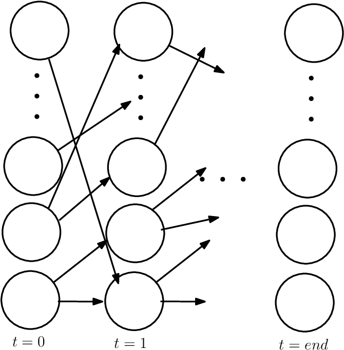
Let $\mathcal{H}$ be hypothesis class over a domain set $\mathcal{X}$. A learning algorithm receives, in an on-line fashion, a series of labeled examples $(x,f(x))$, where $f$ is the true hypothesis. The goal of the algorithm is to return a hypothesis $h\in\mathcal{H}$ that is close to $f.$ Any bounded-memory algorithm can be described using a branching program (see Figure 1(a)), which is a layered graph. Each layer corresponds to a time step, i.e., number of examples received so far. Each layer contains all the possible memory states. If the algorithm uses $b$ bits, then there are $2^{b}$ memory states. One can learn any class $\mathcal{H}$ over domain $\mathcal{X}$ with $O(\log|\mathcal{H}|)$ examples and $O(\log|\mathcal{X}|\log|\mathcal{H}|)$ memory bits. Thus, a learning algorithm that uses much less memory bits, $o(\log|\mathcal{X}|\cdot\log|\mathcal{H}|)$ bits, is called a bounded-memory algorithm.

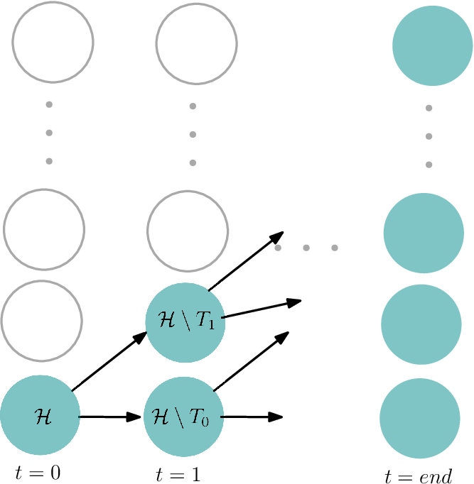
One of the main contribution of this work is designing a general learning algorithm that uses a bounded amount of bits. This algorithm saves in memory a subset of hypotheses $T$ that, with high probability, contains the correct hypothesis $f$. At the beginning of the algorithm, $T$ contains all the hypotheses in $\mathcal{H}$. At each step the algorithm reduces a large fraction of $T$ while only using a few bits. The algorithm acts differently depending on whether $T$ contains a large subset of hypotheses that are close to each other or not. We call the former case tightness, as formalized next.

Two hypotheses $h_{1},h_{2}\in\mathcal{H}$ are $\epsilon$-close if $\Pr_{x\sim\mathcal{D}}(h_{1}(x)\neq h_{2}(x))\leq\epsilon,$ where $\mathcal{D}$ is the known distribution over the examples²² 2 For ease of presentation, in the rest of the paper we focus on the case that $\mathcal{D}=\mathcal{U}$ is the uniform distribution.. An $\epsilon$-ball with center $h\in\mathcal{H}$ is the set $B_{h}(\epsilon)=\{h^{\prime}\in\mathcal{H}\,|\,h^{\prime}\text{ and }h\text{ are }\epsilon\text{-close}\}.$ A subset $T\subseteq\mathcal{H}$ is $(\alpha,\epsilon)$-tight if there is a hypothesis $h$ with $|T\cap B_{h}(\epsilon)|\geq\alpha|T|$. Note that $\alpha$ and $\epsilon$ are related as large $\epsilon$ implies that $\alpha$ is also large. At each step, the algorithm distinguishes between the cases that $T$ is tight and $T$ is not tight and handle each case separately.

$T$ is $(\alpha,\epsilon)$-tight: in this case there is a hypothesis $h$ with $|T\cap B_{h}(\epsilon)|\geq\alpha|T|$. The algorithm tests if $h$ is $\epsilon$-close to the correct hypothesis $f$. This is done using a few random examples, as described in Algorithm 1. If $h$ is $\epsilon$-close, then the algorithm halts. Otherwise, the algorithm can safely delete $B_{h}(\epsilon)$ from $T$, i.e., in this case the algorithm can reduce many, $\alpha|T|$, hypotheses from $T$.

$T$ is not $(\alpha,\epsilon)$-tight: for this case we use ideas from graph theory. A hypothesis class $\mathcal{H}$ over domain $\mathcal{X}$ can be represented as a bipartite-graph in the following way. The vertices are the hypotheses $\mathcal{H}$ and the examples $\mathcal{X}$, and the edges connect every hypothesis $h\in\mathcal{H}$ to an example $x\in\mathcal{X}$ if and only if $h(x)=1.$ We call the appropriate bipartite graph the hypotheses graph of $\mathcal{H}.$ For any graph $(A,B,E)$, the density between sets of vertices $S\subseteq A$ and $T\subseteq B$ is $d(S,T)=\frac{e(S,T)}{|S||T|}$, where $e(S,T)$ is the number of edges with a vertex in $S$ and a vertex in $T$. In case that $T$ contains only one vertex $T=\{v\}$, we simply write $d(S,v)$.

For any heavy-weight $S$ (i.e., $|S|\geq\alpha|\mathcal{X}|$ under the uniform distribution) the density $d(S,f)$ between $S$ and the correct hypothesis $f$ can be easily estimated without saving many bits in memory (see Algorithm 2). Hence, the algorithm can rule out from $T$ any hypotheses $h\in T$ with $d(S,h)\not\approx d(S,f)$. In cases where there are two large disjoint subsets $T_{0},T_{1}\subseteq T$, $|T_{0}|,|T_{1}|\geq\alpha|T|$ with

either $T_{0}$ or $T_{1}$ can be ruled out from $T.$ So the algorithm is able to delete $\alpha|T|$ hypotheses from $|T|$ while only using a small number of memory bits. For classes that satisfy the separability property, as will be formalized in the next section, Equation ${(\ref{eq:local_separability})}$ holds. In Section 5 we also show examples of classes (e.g., decision lists) that satisfy the separability property.

The algorithm uses an oracle ³³ 3 There is such an oracle for any separable class, see Section 4. For the entire algorithm to be bounded memory, it is assumed that the oracle is also bounded memory, which is true for all the classes presented in this paper. that provides the following functionality for any subset of hypotheses $T\subseteq\mathcal{H}$:

• •

  If $T$ is $(\alpha,\epsilon)$-tight, the oracle provides a proof for this by returning $h\in\mathcal{H}$ with $|T\cap B_{h}(\epsilon)|\geq\alpha|T|.$

• •

  If $T$ is not $(\alpha,\epsilon)$-tight, the oracle returns $S\subseteq\mathcal{X},T_{1},T_{0}\subseteq T,d_{0},d_{1}\in\mathbb{R}$ with $|S|\geq\alpha|\mathcal{X}|$, $|T_{0}|,|T_{1}|\geq\mathrm{poly}(\alpha)\cdot|T|$ and $d_{1}-d_{0}\geq\Omega(\alpha)\cdot|S|$ such that $h\in T_{0}$ implies $e(h,S)\leq d_{0}$ and $h\in T_{1}$ implies $e(h,S)\geq d_{1}$.

In Section 5 we show how to efficiently, both in time and in memory, implement this oracle for specific classes. The algorithm also uses the following subroutines: (i) Is-close$(h,\epsilon,k)$ — tests whether $h$ is $\epsilon$-close to the correct hypothesis with error exponentially small in $k$. See Algorithm 1. (ii) Estimate$(S,\tau,k)$ — estimates $d(S,f)$ up to an additive error of $\tau$ with error exponentially small in $k$. See Algorithm 2. The correctness of the subroutines is stated and proved in the Appendix.

The general bounded-memory algorithm is described in Algorithm 3 and a graphical representation of it as a branching program appears in Figure 1(b). The algorithm proceeds as follows. At each step we maintain a set $T\subseteq\mathcal{H}$ of candidates to be the correct hypothesis. In Line 3 we initialize $T$ to be $\mathcal{H},$ the entire hypothesis class. In Line 5 the algorithm calls the oracle and if $T$ is $(\alpha,\epsilon)$-tight, in Line 6 it tests whether the hypothesis $h$ returned by the oracle is $\epsilon$-close to the correct hypothesis. If $h$ is close enough to the correct hypothesis, the algorithm halts and returns $h,$ otherwise the algorithm can safely remove all the hypotheses that are $\epsilon$-close to $h$, as done in Line 9. If $T$ is not $(\alpha,\epsilon)$-tight, then in Line 12 the algorithm calls the oracle to find $S,T_{1},T_{0},d_{0},d_{1}$. In Line 13 the algorithm estimates $d(S,f)$, where $f$ is the correct hypothesis, and tests whether it is closer to $d_{0}$ or $d_{1}.$ Then, it is able to delete $T_{0}$ or $T_{1}$ according to the value of $r$ in Lines 15, 17.

In the next section we introduce the separability property, which uses similar terms as in mixing. For classes that satisfy this property the oracle can be implemented and therefore the algorithm functions correctly. We prove that several natural classes satisfy this property, for example, the class of decision lists. Thus, it can be learned with bounded memory. An interesting feature of the general bounded-memory algorithm is that it is also a statistical query algorithm, as we describe next, and thus robust to random noise.

In this section we formally define the separability property as a combinatorial condition of a bipartite graph. This property is closely related to the mixing property defined in [15]. Recall that hypothesis class can be viewed as a bipartite graph using the hypotheses graph. We first define closeness and tight in the language of graph theory.

In what follow we fix a bipartite graph $(A,B,E)$. Two vertices $h_{1},h_{2}\in A$ are $\epsilon$-close if $|N(h_{1})\triangle N(h_{2})|\leq\epsilon|B|$, where $N(h)$ denotes the set of neighbors of vertex $h$ and $\triangle$ denotes the symmetric difference. Similar to the previous section we define the $\epsilon$-ball with center $h\in A$ as the set $B_{h}(\epsilon)=\{h^{\prime}\in A\,|\,h^{\prime}\text{ and }h\text{ are }\epsilon\text{-close}\}.$ A subset $T\subseteq A$ is $(\alpha,\epsilon)$-tight if there is a hypothesis $h$ with $|T\cap B_{h}(\epsilon)|\geq\alpha|T|$.

In the previous section we used Equation $(\ref{eq:local_separability})$, which is a local requirement on each hypothesis. We relax this requirement and instead require a weaker global requirement, as stated in the following definition.

A hypothesis class is $(\alpha,\epsilon)$-separable if its hypotheses graph is $(\alpha,\epsilon)$-separable. Perhaps surprisingly, the global requirement of separability implies the local requirement, as stated in the following claim (see the Appendix for the proof).

The next theorem proves the correctness of Algorithm 3 (the proof appears in the Appendix). For brevity we define $(m,b,\delta,\epsilon)$-bounded memory learning algorithm as an algorithm that uses at most $m$ labeled examples sampled from the uniform distribution, $b$ bits of memory, and returns a hypothesis that is $\epsilon$-close to the correct hypothesis with probability at least $1-\delta.$ We omit the $O$ symbol for simplicity.

If $\alpha^{-2}$ is smaller than $\log|\mathcal{X}|$ we get that Algorithm 3 is indeed a bounded-memory algorithm. On the other hand, the number of samples is increased by a small factor of $\nicefrac{{(\log\log|\mathcal{H}|+\log\nicefrac{{1}}{{\alpha}})}}{{\alpha^{5}}}$ compared to the $\log|\mathcal{H}|$ examples needed in case $\mathrm{VCdim}(\mathcal{H})\approx\log|\mathcal{H}|$. One might wonder how the number of samples does not depend on $\epsilon$. Taking a closer look, we observe that this is not the case as generally $\epsilon$ is lower bounded by a function of $\alpha$. Take for example $T$ that contains hypotheses that disagree on exactly $\alpha^{2}$ of the examples. If $\epsilon<\alpha^{2}$, then $T$ is not $(\alpha,\epsilon)$-tight thus the class is not $(\alpha,\epsilon)$-separable.

In this section we present a few natural classes and prove they are separable. This implies, using Theorem 3, that they are properly learnable with bounded memory.

In this paper we introduced the concept of separability, which is similar to non-mixing, suggested a general bounded memory algorithm, proved its correctness for classes that are separable, and proved it is also an sq-algorithm. We also derived time-efficient bounded memory algorithms for three natural classes: threshold functions, equal-piece classifiers, and decision lists.

Several questions remain open. One question is to prove that other classes are separable and thus can be learned with the general bounded memory algorithm. A second open problem is to extend our work to the case of an unknown distribution over the examples. Another open problem is to close the gap between separability and non-mixing.

References

- [1] Paul Beame, Shayan Oveis Gharan, and Xin Yang. Time-space tradeoffs for learning from small test spaces: Learning low degree polynomial functions. arXiv preprint arXiv:1708.02640, 2017.
- [2] Avrim Blum, Merrick Furst, Jeffrey Jackson, Michael Kearns, Yishay Mansour, and Steven Rudich. Weakly learning dnf and characterizing statistical query learning using fourier analysis. In Symposium on Theory of Computing (STOC), 1994, pages 253–262, 1994.
- [3] Anselm Blumer, Andrzej Ehrenfeucht, David Haussler, and Manfred K Warmuth. Occam’s razor. Information processing letters, 24(6):377–380, 1987.
- [4] Aditi Dhagat and Lisa Hellerstein. PAC learning with irrelevant attributes. In Foundations of Computer Science, 1994 Proceedings., 35th Annual Symposium on, pages 64–74. IEEE, 1994.
- [5] Carlos Domingo and Osamu Watanabe. Madaboost: A modification of adaboost. In Proceedings of the Thirteenth Annual Conference on Computational Learning Theory, pages 180–189. Morgan Kaufmann Publishers Inc., 2000.
- [6] Thomas Eiter, Toshihide Ibaraki, and Kazuhisa Makino. Decision lists and related boolean functions. Theoretical Computer Science, 270(1-2):493–524, 2002.
- [7] Vitaly Feldman. A general characterization of the statistical query complexity. In Satyen Kale and Ohad Shamir, editors, Proceedings of the 2017 Conference on Learning Theory, volume 65 of Proceedings of Machine Learning Research, pages 785–830, Amsterdam, Netherlands, 07–10 Jul 2017. PMLR.
- [8] Sally Floyd. Space-bounded learning and the vapnik-chervonenkis dimension. In Proceedings of the second annual workshop on Computational learning theory, pages 349–364. Morgan Kaufmann Publishers Inc., 1989.
- [9] Sumegha Garg, Ran Raz, and Avishay Tal. Extractor-based time-space lower bounds for learning. arXiv preprint arXiv:1708.02639, 2017.
- [10] Michael Kearns. Efficient noise-tolerant learning from statistical queries. Journal of the ACM (JACM), 45(6):983–1006, 1998.
- [11] Adam R Klivans and Rocco A Servedio. Toward attribute efficient learning of decision lists and parities. Journal of Machine Learning Research, 7(Apr):587–602, 2006.
- [12] Gillat Kol, Ran Raz, and Avishay Tal. Time-space hardness of learning sparse parities. In Symposium on Theory of Computing (STOC), 2017, pages 1067–1080, 2017.
- [13] Nick Littlestone and Manfred Warmuth. Relating data compression and learnability. Technical report, Technical report, University of California, Santa Cruz, 1986.
- [14] Philip M Long and Rocco Servedio. Attribute-efficient learning of decision lists and linear threshold functions under unconcentrated distributions. In Advances in Neural Information Processing Systems, pages 921–928, 2007.
- [15] Dana Moshkovitz and Michal Moshkovitz. Mixing implies lower bounds for space bounded learning. In Conference on Learning Theory, pages 1516–1566, 2017.
- [16] Dana Moshkovitz and Michal Moshkovitz. Entropy samplers and strong generic lower bounds for space bounded learning. In LIPIcs-Leibniz International Proceedings in Informatics, volume 94. Schloss Dagstuhl-Leibniz-Zentrum fuer Informatik, 2018.
- [17] Michal Moshkovitz and Naftali Tishby. Mixing complexity and its applications to neural networks. arXiv preprint arXiv:1703.00729, 2017.
- [18] Ziv Nevo and Ran El-Yaniv. On online learning of decision lists. Journal of Machine Learning Research, 3(Oct):271–301, 2002.
- [19] Ran Raz. Fast learning requires good memory: A time-space lower bound for parity learning. In Foundations of Computer Science (FOCS), 2016 IEEE 57th Annual Symposium on, pages 266–275. IEEE, 2016.
- [20] Ran Raz. A time-space lower bound for a large class of learning problems. In Foundations of Computer Science (FOCS), 2017 IEEE 58th Annual Symposium on, 2017.
- [21] Ronald L Rivest. Learning decision lists. Machine learning, 2(3):229–246, 1987.
- [22] Frank Rosenblatt. The perceptron, a perceiving and recognizing automaton Project Para. Cornell Aeronautical Laboratory, 1957.
- [23] Robert E Schapire. The strength of weak learnability. Machine learning, 5(2):197–227, 1990.
- [24] Shai Shalev-Shwartz and Shai Ben-David. Understanding machine learning: From theory to algorithms. Cambridge university press, 2014.
- [25] Ohad Shamir. Fundamental limits of online and distributed algorithms for statistical learning and estimation. In Advances in Neural Information Processing Systems, pages 163–171, 2014.
- [26] Jacob Steinhardt, Gregory Valiant, and Stefan Wager. Memory, communication, and statistical queries. In Conference on Learning Theory, pages 1490–1516, 2016.
- [27] Worldometers. Internet live statistics. http://www.internetlivestats.com/, 2019.
Appendix A Outline
This appendix contains several technical claims: the classes presented in the main text are separable (Section B), time-efficient implementation of the general algorithm to these classes (Section C), correctness proof of the general algorithm for classes that satisfy separability (Section D), and a proof that the general algorithm is also a statistical query algorithm (Section E).
Appendix B Separability
In this section we formally prove that all classes introduced in the main text are in fact separable.
B.1 The class of threshold functions is separable
Theorem 6.
For any , the class is -separable.
Proof.
Fix and which is not -tight. We want to find with and with such that