跳到论文正文
W Papers独立论文阅读器 arXiv:1712.03462 论文正文 计算阅读时间 · 0%
引用这篇论文根据当前论文元数据生成,正式投稿前建议核对。


License: arXiv.org perpetual non-exclusive license
arXiv:1712.03462v1 [gr-qc] 10 Dec 2017

UFIFT-QG-17-05, CCTP-2017-10

From Non-trivial Geometries to Power Spectra and Vice Versa

D. J. Brooker1∗, N. C. Tsamis2⋆ and R. P. Woodard1†

1 Department of Physics, University of Florida,
Gainesville, FL 32611, UNITED STATES

2 Institute of Theoretical Physics & Computational Physics,
Department of Physics, University of Crete,
GR-710 03 Heraklion, HELLAS

ABSTRACT

We review a recent formalism which derives the functional forms of the primordial – tensor and scalar – power spectra of scalar potential inflationary models. The formalism incorporates the case of geometries with non-constant first slow-roll parameter. Analytic expressions for the power spectra are given that explicitly display the dependence on the geometric properties of the background. Moreover, we present the full algorithm for using our formalism, to reconstruct the model from the observed power spectra. Our techniques are applied to models possessing “features” in their potential with excellent agreement.

PACS numbers: 04.50.Kd, 95.35.+d, 98.62.-g

∗ e-mail: djbrooker@ufl.edu

⋆ e-mail: tsamis@physics.uoc.gr

† e-mail: woodard@phys.ufl.edu

1 Introduction

We shall assume that inflation is described by general relativity minimally coupled to a scalar field φ⁡(x)\varphi(x) with a self-interacting potential V⁡(φ)V(\varphi): 11 1 Hellenic indices take on spacetime values while Latin indices take on space values. Our metric tensor gμ​νg_{\mu\nu} has spacelike signature (−+++)(-\,+\,+\,+) and our curvature tensor equals Rβ​μ​να≡Γν​β,μα+Γμ​ρα​Γν​βρ−(μ↔ν)R^{\alpha}_{~\beta\mu\nu}\equiv\Gamma^{\alpha}_{~\nu\beta,\mu}+\Gamma^{\alpha}_{~\mu\rho}\,\Gamma^{\rho}_{~\nu\beta}-(\mu\leftrightarrow\nu).

ℒ=1​−g16​π​G​R​−g−12​∂μφ​∂νφ​gμ​ν​−g−V⁡(φ)​−g.\mathcal{L}\,=\,\frac{1\sqrt{-g}}{16\pi G}R\sqrt{-g}-\frac{1}{2}\partial_{\mu}\varphi\,\partial_{\nu}\varphi\,g^{\mu\nu}\sqrt{-g}-V(\varphi)\,\sqrt{-g}\;\;. (1)

The theory described by (1) predicts the generation of tensor [1] and scalar [2] perturbations. These predictions provide the main test for the validity of such models [3, 4] as well as the reconstruction of the potential V⁡(φ)V(\varphi) [5]. The class of spacetimes under consideration is characterized by the scale factor a⁡(t)a(t) and, hence, the Hubble parameter H⁡(t)H(t) and the first slow-roll parameter ϵ⁡(t)\epsilon(t):

d​s2=−d​t2+a2​(t)​d​x→⋅d​x→⟹H⁡(t)≡a˙a,ϵ⁡(t)≡−H˙H2.ds^{2}=-dt^{2}+a^{2}(t)\,d\vec{x}\!\cdot\!d\vec{x}\quad\Longrightarrow\quad H(t)\equiv\frac{\dot{a}}{a}\quad,\quad\epsilon(t)\equiv-\frac{\dot{H}}{H^{2}}\;\;. (2)

We shall study the tree order tensor and scalar primordial power spectra, Δh2​(k)\Delta^{2}_{h}(k) and Δℛ2​(k)\Delta^{2}_{\mathcal{R}}(k) respectively. They are known in terms of the constant amplitudes approached by their mode functions, u⁡(t,k)u(t,k) and v⁡(t,k)v(t,k) respectively, after the first horizon crossing time tkt_{k} [6]:

Δh2​(k)\displaystyle\Delta^{2}_{h}(k) =\displaystyle\!\!=\!\! k32​π2×32​π​G×2×|u⁡(t,k)|t≫tk2,\displaystyle\frac{k^{3}}{2\pi^{2}}\times 32\pi G\times 2\times\Big|u(t,k)\Big|^{2}_{t\gg t_{k}}\;\;, (3)
Δℛ2​(k)\displaystyle\Delta^{2}_{\mathcal{R}}(k) =\displaystyle\!\!=\!\! k32​π2×4​π​G×|v⁡(t,k)|t≫tk2,\displaystyle\frac{k^{3}}{2\pi^{2}}\times 4\pi G\times\Big|v(t,k)\Big|^{2}_{t\gg t_{k}}\;\;, (4)

where k=H⁡(tk)​a​(tk)k=H(t_{k})a(t_{k}). The time evolution equations obeyed by these mode functions:

u¨+3​H​u˙+k2a2​u=0\displaystyle\ddot{u}+3H\dot{u}+\frac{k^{2}}{a^{2}}u=0 , u​u˙∗−u˙​u∗=ia3,\displaystyle u\dot{u}^{*}\!-\dot{u}u^{*}=\frac{i}{a^{3}}\;\;, (5)
v¨+(3​H+ϵ˙ϵ)​v˙+k2a2​v=0\displaystyle\ddot{v}+\Bigl(3H+\frac{\dot{\epsilon}}{\epsilon}\Bigr)\dot{v}+\frac{k^{2}}{a^{2}}v=0 , v​v˙∗−v˙​v∗=iϵ​a3,\displaystyle v\dot{v}^{*}\!-\dot{v}v^{*}=\frac{i}{\epsilon a^{3}}\;\;, (6)

cannot be solved exactly and we must resort to complicated numerical techniques for realistic inflationary models.

It is evident from equations (5-6) that constant solutions exist when k2a2\frac{k^{2}}{a^{2}} becomes negligible. Exact solutions are known for ϵ⁡(t)=ϵ0\epsilon(t)=\epsilon_{0}:

u0​(t,k,ϵ0)\displaystyle u_{0}(t,k;\epsilon_{0}) =\displaystyle\!\!=\!\! π4​k​a2​(t)​z​(t)​Hν(1)​(z⁡(t)),v0​(t,k,ϵ0)=u0​(t,k,ϵ0)ϵ0,\displaystyle\sqrt{\frac{\pi}{4ka^{2}(t)}\,z(t)}\;H^{(1)}_{\nu}\bigl(z(t)\bigr)\quad,\quad v_{0}(t,k;\epsilon_{0})\,=\,\frac{u_{0}(t,k;\epsilon_{0})}{\sqrt{\epsilon_{0}}}\;\;,
z⁡(t)\displaystyle z(t) ≡\displaystyle\!\!\equiv\!\! k(1−ϵ0)​H​(t)​a​(t),ν≡12+11−ϵ0.\displaystyle\frac{k}{(1-\epsilon_{0})H(t)\,a(t)}\quad,\quad\nu\,\equiv\,\frac{1}{2}+\frac{1}{1-\epsilon_{0}}\;\;. (7)

However, no constant value of ϵ⁡(t)\epsilon(t) seems to be consistent with the data, cf. Figure 12 of [7]. Achieving more realism involves consideration of geometries with non-constant ϵ⁡(t)\epsilon(t) [8, 9]. Therefore, we must go beyond the leading slow-roll approximation – ϵ⁡(t)=ϵ0≪1,ϵ′​(t)=0\epsilon(t)=\epsilon_{0}\ll 1\;,\epsilon^{\prime}(t)=0 – to the power spectra:

Δh2​(k)|leading=16​G​H2​(tk)π,Δℛ2​(k)|leading=G​H2​(tk)π​ϵ​(tk).\Delta^{2}_{h}(k)\Big|_{\rm leading}=\frac{16GH^{2}(t_{k})}{\pi}\quad,\quad\Delta^{2}_{\mathcal{R}}(k)\Big|_{\rm leading}=\frac{GH^{2}(t_{k})}{\pi\epsilon(t_{k})}\;\;. (8)

which, although qualitatively accurate over most of the observed spectrum, does not provide a good description of features, for example, the power deficit at ℓ=22\ell=22 and the excess at ℓ=40\ell=40 visible in Figure 1 [10]. 22 2 It should be noted that these are 3​σ3\sigma deviations and more accuracy is needed to establish them as true physical results.

Refer to caption
Figure 1: The PLANCK 2015 [10] strength of temperature variations (vertical) against their angular sizes (horizontal). The line is the standard cosmological model, the dots are the data.

The deviations do not disappear when we consider the local slow roll approximation – ϵ⁡(t)=ϵ0,ϵ′​(t)=0\epsilon(t)=\epsilon_{0}\;,\epsilon^{\prime}(t)=0 – to the power spectra:

Δh2​(k)|local=16​G​H2​(tk)π×C⁡[ϵk],Δℛ2​(k)|local=G​H2​(tk)π​ϵ​(tk)×C⁡[ϵk],\Delta^{2}_{h}(k)\Big|_{\rm local}=\frac{16GH^{2}(t_{k})}{\pi}\times C[\epsilon_{k}]\quad,\quad\Delta^{2}_{\mathcal{R}}(k)\Big|_{\rm local}=\frac{GH^{2}(t_{k})}{\pi\epsilon(t_{k})}\times C[\epsilon_{k}]\;\;, (9)

where the local slow-roll correction factor C⁡[ϵ0]C[\epsilon_{0}] is:

C⁡[ϵ0]=1π​Γ2​(12+1−ϵ0)​[2​(−ϵ0)]21−ϵ0≈ 1−ϵ0,C[\epsilon_{0}]\,=\,\frac{1}{\pi}\,\Gamma^{2}\Big(\frac{1}{2}\!+\!\frac{1}{1\!-\!\epsilon_{0}}\Big)\Bigl[2(1\!-\!\epsilon_{0})\Bigr]^{\frac{2}{1-\epsilon_{0}}}\,\approx\,1-\epsilon_{0}\;\;, (10)

and its graph can be seen in Figure 2.

Refer to caption
Refer to caption
Figure 2: The left hand graph shows the local slow-roll constant ϵ\epsilon correction factor C⁡(ϵ)C(\epsilon) (solid blue), which was defined in expression (10). Also shown is its global approximation of  1−ϵ\,1-\epsilon\, (dashed yellow) over the full inflationary range of  0≤ϵ<1\,0\leq\epsilon<1. The right hand graph shows C⁡(ϵ)C(\epsilon) (solid blue) versus the better approximation of  1−0.55​ϵ\,1-0.55\epsilon (large dots) relevant to the range  0≤ϵ<0.02\,0\leq\epsilon<0.02\, favoured by current data.

That said, we set some goals [11] when trying to develop a formalism that incorporates more generic inflationary models and goes beyond (8, 9) in a non-trivial and potentially quite interesting way: 33 3 We are not concerned in this study with quantum corrections to the power spectra as their loop counting parameter is very small (G​H2<<10−11)(GH^{2}<<10^{-11}) and it is not clear what operators represent them at loop order [12].
∙\bullet\; The class of geometries studied must incorporate those with a varying ϵ⁡(t)\epsilon(t). In particular, we should correctly describe transient effects in the power spectra due to the non-constancy of ϵ⁡(t)\epsilon(t); these will eventually reside in the non-local dependence of the power spectrum on ϵ⁡(t)\epsilon(t).
∙\bullet\; The formalism must be bi-directional:
(i) from spacetime {a(t)⇒H(t)⇒ϵ(t)}\{a(t)\Rightarrow H(t)\Rightarrow\epsilon(t)\} to spectrum {Δℛ2​(k),Δh2​(k)}\{\Delta^{2}_{\mathcal{R}}(k),\Delta^{2}_{h}(k)\} and,
(ii) from spectrum {Δℛ2​(k),Δh2​(k)}\{\Delta^{2}_{\mathcal{R}}(k),\Delta^{2}_{h}(k)\} to spacetime {a(t)⇒H(t)⇒ϵ(t)}\{a(t)\Rightarrow H(t)\Rightarrow\epsilon(t)\}.
∙\bullet\; The formalism must be such that if numerical methods need to be employed, they will be as efficient as possible.

2 From the Geometry to the CMBR

In this Section we describe the steps that lead to the generalized expressions for the tensor and scalar primordial power spectra. Because these steps are very similar in both cases, we shall be more detailed for the tensor case and rather compact for the scalar case.
* The Tensor Spectrum
- Step 1: The optimal evolution variables.
Elementary inspection of (3) shows that the relevant quantity is not u⁡(t,k)u(t,k) evolving via (5) but M⁡(t,k)≡|u⁡(t,k)|2M(t,k)\equiv|u(t,k)|^{2} evolving according to [13, 14]:

M′′M+(3−ϵ)​M′M+2​k2a2​H2−12​(M′M)2−12​a6​H2​M2=0.\frac{M^{\prime\prime}}{M}+(3-\epsilon)\frac{M^{\prime}}{M}+\frac{2k^{2}}{a^{2}H^{2}}-\frac{1}{2}\left(\frac{M^{\prime}}{M}\right)^{2}-\frac{1}{2a^{6}H^{2}M^{2}}=0\;\;. (11)

We have converted from co-moving time tt to the number of ee-foldings from the beginning of inflation nn:

n≡ln[a⁡(t)ai],dd​t=Hdd​n,′≡dd​n.n\equiv\ln\!\left[\frac{a(t)}{a_{i}}\right]\quad,\quad\frac{d}{dt}=H\frac{d}{dn}\quad,\quad^{\prime}\equiv\frac{d}{dn}\;\;. (12)

An evolution equation like (11) is preferable since it avoids the need to take into account the oscillating phases of the mode functions that enter into the evolution equations (5-6).
- Step 2: Decomposition into “background” ×\times “residual”.
The next step is to write our variable M⁡(t,k)M(t,k) in the form of an appropriate background M0​(t,k)M_{0}(t,k) times a residual h⁡(n,k)h(n,k):

M⁡(t,k)≡M0​(t,k)×exp⁡[−12​h​(n,k)].M(t,k)\equiv M_{0}(t,k)\times\exp\!\left[-\frac{1}{2}h(n,k)\right]\;\;. (13)

The background is chosen by requiring that it captures the main effect. The residual is to be determined from the evolution equation it satisfies.
- Step 3: The background choice.
The background should incorporate the main effect by taking simultaneously into account:
(i) the relative success of the slow-roll approximation,
(ii) the need to allow for time dependent ϵ⁡(t)\epsilon(t),
(iii) the constancy that the physical mode function M⁡(t,k)M(t,k) eventually achieves past first horizon crossing; since ϵ⁡(t)\epsilon(t) continues to evolve, so does M0​(t,k)M_{0}(t,k) and its time dependence should be eliminated by a compensating time dependence in the residual h⁡(n,k)h(n,k) to obtain the required constancy of the full mode function M⁡(t,k)M(t,k).
With these requirements in mind, we choose:

∀t<tk\displaystyle\forall t<t_{k} :\displaystyle\!\!\!: M0​(t,k)​from​instantaneously​constant​ϵ​solution,\displaystyle M_{0}(t,k)\;{\rm from\;instantaneously\;constant\;\epsilon\;solution}\;\;, (14)
∀t>tk\displaystyle\forall t>t_{k} :\displaystyle\!\!\!: M0​(t,k)​from​constant​ϵk​solution.\displaystyle M_{0}(t,k)\;{\rm from\;constant\;\epsilon_{k}\;solution}\;\;. (15)

This can be mathematically expressed as follows:

M0​(t,k)=θ⁡(tk−t)​Minst​(t,k)+θ⁡(t−tk)​M¯inst​(t,k),M_{0}(t,k)\,=\,\theta(t_{k}-t)\;M_{\rm inst}(t,k)\,+\,\theta(t-t_{k})\;{\overline{M}}_{\rm inst}(t,k)\;\;, (16)

with the understanding that the instantaneously constant ϵ\epsilon solution is:

Minst​(t,k)≡z⁡(t,k)​ℋ​(ν⁡(t),z⁡(t,k))2​k​a2​(t),ℋ⁡(ν,z)≡π2​|Hν(1)​(z)|2,M_{\rm inst}(t,k)\,\equiv\,\frac{z(t,k)\;\mathcal{H}(\nu(t),z(t,k))}{2k\,a^{2}(t)}\quad,\quad\mathcal{H}(\nu,z)\equiv\frac{\pi}{2}\Big|H^{(1)}_{\nu}(z)\Big|^{2}\;\;, (17)

with the usual definitions:

ν⁡(t)≡12+11−ϵ⁡(t),z⁡(t,k)≡k[1−ϵ⁡(t)]​H​(t)​a​(t).\nu(t)\equiv\frac{1}{2}+\frac{1}{1-\epsilon(t)}\quad,\quad z(t,k)\equiv\frac{k}{[1-\epsilon(t)]H(t)\,a(t)}\;\;. (18)

From first horizon crossing onwards, the backround is the constant ϵ\epsilon solution for ϵ⁡(t)=ϵk\epsilon(t)=\epsilon_{k}:

M¯inst​(t,k)≡z¯​(t,k)​ℋ​(ν⁡(t),z¯​(t,k))2​k​a¯2​(t).{\overline{M}}_{\rm inst}(t,k)\,\equiv\,\frac{{\overline{z}}(t,k)\;\mathcal{H}(\nu(t),{\overline{z}}(t,k))}{2k\,{\overline{a}}^{2}(t)}\;\;. (19)

In terms of the number of ee-foldings from first horizon crossing Δ​n≡n−nk\;\Delta n\equiv n-n_{k}\, the geometrical parameters of (19) are:

a¯​(n)=a⁡(n)=ak​eΔ​n,H¯​(n)=Hk​e−ϵk​Δ​n,ϵ¯​(n)=ϵk.\overline{a}(n)=a(n)=a_{k}e^{\Delta n}\quad,\quad\overline{H}(n)=H_{k}\,e^{-\epsilon_{k}\Delta n}\quad,\quad\overline{\epsilon}(n)=\epsilon_{k}\;\;. (20)

- Step 4: The primordial tensor power spectrum.
The late time limit of M0​(t,k)M_{0}(t,k) is:

limt≫tkM0​(t,k)=limt≫tkz¯​(t,k)2​k​a¯2​(t)​ℋ​(ν⁡(t),z⁡(t,k))=H2​(nk)2​k3×C⁡[ϵ⁡(nk)].\lim_{t\gg t_{k}}M_{0}(t,k)\,=\,\lim_{t\gg t_{k}}\frac{{\bar{z}}(t,k)}{2k\,{\bar{a}}^{2}(t)}\;{\cal H}(\nu(t),z(t,k))\,=\,\frac{H^{2}(n_{k})}{2k^{3}}\times C[\epsilon(n_{k})]\;\;. (21)

The physical object of interest is the tensor power spectrum (3) which in view of (21) now equals:

Δh2​(k)\displaystyle\Delta^{2}_{h}(k) =\displaystyle\!\!=\!\! k32​π2×32​π​G×2×M0​(t,k)​e−12​h​(n,k)|t≫tk,\displaystyle\frac{k^{3}}{2\pi^{2}}\times 32\pi G\times 2\times M_{0}(t,k)\,e^{-\frac{1}{2}h(n,k)}\Big|_{t\gg t_{k}}\;\;, (22)
=\displaystyle\!\!=\!\! 16​G​H2​(nk)π×C⁡[ϵ⁡(nk)]×eτ​[ϵ]​(k).\displaystyle\frac{16GH^{2}(n_{k})}{\pi}\times C[\epsilon(n_{k})]\times e^{\tau[\epsilon](k)}\;\;. (23)

The non-local correction factor τ​[ϵ]​(k)\tau[\epsilon](k) to the tensor power spectrum is seen to be:

τ⁡[ϵ]​(k)≡limn≫nk[−12​h​(n,k)].\tau[\epsilon](k)\,\equiv\,\lim_{n\gg n_{k}}\left[-\frac{1}{2}h(n,k)\right]\;\;. (24)

- Step 5: The residual evolution equation.
In terms of the natural frequency of the system: 44 4 When ω∼1\omega\sim 1 we have about one oscillation per ee-folding.

ω⁡(n,k)≡1a3​(t)​H​(t)​M0​(t,k),\omega(n,k)\equiv\frac{1}{a^{3}(t)\,H(t)\,M_{0}(t,k)}\;\;, (25)

and upon substituting the generic relation (13), we can express (11) as follows:

h′′−ω′ω​h′+ω2​h=14​h′ 2−ω2​(eh−1−h)+Sh.h^{\prime\prime}-\frac{\omega^{\prime}}{\omega}h^{\prime}+\omega^{2}h\,=\,\frac{1}{4}h^{\prime\,2}-\omega^{2}\Big(e^{h}-1-h\Big)\,+\,S_{h}\;\;. (26)

This is – up to the non-linearities – an equation of a damped oscillator driven by the tensor source ShS_{h}:

Sh≡−2​(ω′ω)′+(ω′ω)2+2​ϵ′−(3−ϵ)2+4​k2a2​H2−ω2.S_{h}\,\equiv\,-2\left(\frac{\omega^{\prime}}{\omega}\right)^{\prime}+\left(\frac{\omega^{\prime}}{\omega}\right)^{\!\!2}+2\epsilon^{\prime}-(3-\epsilon)^{2}+\frac{4k^{2}}{a^{2}H^{2}}-\omega^{2}\;\;. (27)

In [14] we have been able to solve for the retarded Green’s function Gh​(n,m)G_{h}(n;m) of the linear differential operator DhD_{h} that appears on the left hand side of (26):

Dh\displaystyle D_{h} ≡\displaystyle\!\!\equiv\!\! ∂n2−ω′ω∂n+ω2⟹\displaystyle\partial_{n}^{2}-\frac{\omega^{\prime}}{\omega}\partial_{n}+\omega^{2}\quad\Longrightarrow\quad (28)
Gh​(n,m)\displaystyle G_{h}(n;m) =\displaystyle\!\!=\!\! θ⁡(n−m)ω⁡(m,k)​sin⁡[∫0nd​n′​ω​(n′,k)].\displaystyle\frac{\theta(n-m)}{\omega(m,k)}\;\sin\!\left[\int_{0}^{n}dn^{\prime}\;\omega(n^{\prime},k)\right]\;\;. (29)

The above Green’s function is exact and true for any choice of the background M0M_{0}. As a result, we can perturbatively solve (26) with initial value data h⁡(0,k)=h′​(0,k)=0h(0,k)=h^{\prime}(0,k)=0:

h=h1+h2+…,\displaystyle\hskip-59.75095pth\,=\,h_{1}+h_{2}+\dots\;\;, (30)
h1​(n,k)\displaystyle h_{1}(n,k) =\displaystyle\!\!=\!\! ∫0nd​m​Gh​(n,m)​Sh​(m,k),\displaystyle\int_{0}^{n}\!\!dm\,G_{h}(n;m)\,S_{h}(m,k)\;\;, (31)
h2​(n,k)\displaystyle h_{2}(n,k) =\displaystyle\!\!=\!\! ∫0nd​m​Gh​(n,m)​{14​[h1′​(m,k)]2−12​[ω⁡(m,k)​h1​(m,k)]2}.\displaystyle\int_{0}^{n}\!\!dm\,G_{h}(n;m)\left\{\frac{1}{4}\Big[h_{1}^{\prime}(m,k)\Big]^{2}-\frac{1}{2}\Big[\omega(m,k)\,h_{1}(m,k)\Big]^{2}\right\}\;\;.\qquad (32)

- Step 6: The physical approximations.
The non-linear terms in h⁡(n,k)h(n,k) can be safely ignored because no model consistent with the scalar data gives large values of either h⁡(n,k)h(n,k) or h′​(n,k)h^{\prime}(n,k). Thus, we shall only consider the first term (31) in the perturbative solution (30).

Moreover, we should identify the measure of deviation from constant ϵ\epsilon geometries and make a physical approximation that will enable us to achieve a reasonable analytic expression for τ​[ϵ]​(k)\tau[\epsilon](k) which is also accurate. This identification is interval dependent:

∀t<tk\displaystyle\forall t<t_{k} ⇒\displaystyle\!\!\Rightarrow\!\! M0​depends​on​instantaneous​ϵ​(t)\displaystyle M_{0}\;{\rm depends\;on\;instantaneous}\;\epsilon(t) (33)
⇒\displaystyle\!\!\Rightarrow\!\! measures​of​deviation​are:ϵ′,ϵ′′,(ϵ′)2,\displaystyle{\rm measures\;of\;deviation\;are:}\;\epsilon^{\prime}\,,\,\epsilon^{\prime\prime}\,,\,(\epsilon^{\prime})^{2}\;\;,
∀t>tk\displaystyle\forall t>t_{k} ⇒\displaystyle\!\!\Rightarrow\!\! M0​depends​on​constant​ϵk\displaystyle M_{0}\;{\rm depends\;on\;constant}\;\epsilon_{k} (34)
⇒\displaystyle\!\!\Rightarrow\!\! measure​of​deviation​is:Δ​ϵ​(n)=ϵ⁡(n)−ϵ⁡(k).\displaystyle{\rm measure\;of\;deviation\;is:}\;\Delta\epsilon(n)=\epsilon(n)-\epsilon(k)\;\;.

The above deviation measures can be most easily seen by substituting the frequency (25) in the tensor source (27) and noting that the resulting ShS_{h} for t<tkt<t_{k} contains terms proportional to ϵ′\epsilon^{\prime}, ϵ′′\epsilon^{\prime\prime}, (ϵ′)2(\epsilon^{\prime})^{2} but not to Δ​ϵ​(n)\Delta\epsilon(n), while the reverse is true for t>tkt>t_{k}. The approximation consists of:
(i) First extracting the terms proportional to the measures of deviation (33,34) from ShS_{h}.
(ii) Then setting ϵ=0\epsilon=0 throughout given that the range favoured by current data is 0≤ϵ≤0.010\leq\epsilon\leq 0.01.

The approximated Green’s function (29) equals:

limϵ=0Gh​(n,m)\displaystyle\lim_{\epsilon=0}G_{h}(n;m) =\displaystyle\!\!=\!\! θ(n−m)12eΔ​m(1+e2​Δ​m)×\displaystyle\theta(n-m)\;\frac{1}{2}e^{\Delta m}\Big(1+e^{2\Delta m}\Big)\times (35)
×sin⁡[−2​{e−Δ​l−arctan⁡(e−Δ​l)}|mn],Δ​m≡m−nk.\displaystyle\hskip-28.45274pt\times\,\sin\!\Bigg[\!-2\,\Big\{e^{-\Delta l}-\arctan\!\Big(e^{-\Delta l}\Big)\Big\}\Big|_{m}^{n}\Bigg]\quad,\quad\Delta m\equiv m-n_{k}\;\;.\qquad

When concerned with the power spectrum, we must take the late time limit of (35):

limn≫1Gh​(n,m)=12​eΔ​m​(1+e2​Δ​m)​sin⁡[2​e−Δ​m−2​arctan⁡(e−Δ​m)].\lim_{n\gg 1}G_{h}(n;m)\,=\,\frac{1}{2}e^{\Delta m}\Big(1+e^{2\Delta m}\Big)\,\sin\!\left[2e^{-\Delta m}-2\arctan\!\Big(e^{-\Delta m}\Big)\right]\;\;. (36)

Henceforth, for (36) we shall use the compact form:

Gh​(x)=12​(x+x3)​sin⁡[2x−2​arctan⁡(1x)],x≡eΔ​m.G_{h}(x)\,=\,\frac{1}{2}(x+x^{3})\,\sin\!\left[\frac{2}{x}-2\arctan\!\Big(\frac{1}{x}\Big)\right]\quad,\quad x\equiv e^{\Delta m}\;\;. (37)

The approximated source is the sum of the contributions from the two time intervals and their interface:

∀t<tk:\displaystyle\forall t<t_{k}: Sh\displaystyle\!S_{h}\!\!\! =−2​{ϵ′′​(n)​ℰ1​(x)+[ϵ′​(n)]2​ℰ2​(x)+ϵ′​(n)​ℰ3​(x)},\displaystyle=-2\,\Big\{\epsilon^{\prime\prime}(n)\,{\cal E}_{1}(x)+[\epsilon^{\prime}(n)]^{2}\,{\cal E}_{2}(x)+\epsilon^{\prime}(n)\,{\cal E}_{3}(x)\Big\}\;\;, (38)
t=tk:\displaystyle t=t_{k}: Sh\displaystyle\!S_{h}\!\!\! =+2​ϵ′​(nk)​ℰ1​(1)​δ​(n−nk),\displaystyle=+2\,\epsilon^{\prime}(n_{k})\,{\cal E}_{1}(1)\delta(n-n_{k})\;\;, (39)
∀t>tk:\displaystyle\forall t>t_{k}: Sh\displaystyle\!S_{h}\!\!\! =+2​{Δ​ϵ​(n)+4+2​x21+x2​∫nknd​m​Δ​ϵ​(m)}​21+x2.\displaystyle=+2\,\Big\{\Delta\epsilon(n)+\frac{4+2x^{2}}{1+x^{2}}\!\int_{n_{k}}^{n}\!dm\;\Delta\epsilon(m)\Big\}\,\frac{2}{1+x^{2}}\;\;.\qquad (40)

The coefficient functions ℰ1,2,3{\cal E}_{1,2,3} are independent of ϵ\epsilon and are the following combinations of various derivatives of Hankel functions:

ℰ1​(x)\displaystyle\mathcal{E}_{1}(x) =\displaystyle\!\!\!=\!\!\! −1−𝒜0​(x)−ℬ0​(x),\displaystyle-1-\mathcal{A}_{0}(x)-\mathcal{B}_{0}(x)\;\;, (41)
ℰ2​(x)\displaystyle\mathcal{E}_{2}(x) =\displaystyle\!\!\!=\!\!\! 12−𝒜0​(x)−𝒞0​(x)−2​𝒟0​(x)−ℰ0​(x)−12​[+𝒜0​(x)+ℬ0​(x)]2,\displaystyle\frac{1}{2}-\mathcal{A}_{0}(x)-\mathcal{C}_{0}(x)-2\mathcal{D}_{0}(x)-\mathcal{E}_{0}(x)-\frac{1}{2}\Bigl[2\!+\!\mathcal{A}_{0}(x)\!+\!\mathcal{B}_{0}(x)\Bigr]^{2}\;\;,\qquad (42)
ℰ3​(x)\displaystyle\mathcal{E}_{3}(x) =\displaystyle\!\!\!=\!\!\! −1+𝒜0​(x)​ℬ0​(x)+ℬ02​(x)+2​𝒟0​(x)+2​ℰ0​(x),\displaystyle-1+\mathcal{A}_{0}(x)\mathcal{B}_{0}(x)+\mathcal{B}_{0}^{2}(x)+2\mathcal{D}_{0}(x)+2\mathcal{E}_{0}(x)\;\;, (43)

where we have defined:

𝒜0​(x)\displaystyle\mathcal{A}_{0}(x) ≡\displaystyle\!\!\equiv\!\! limϵ=0𝒜(x),𝒜(x)≡∂∂νln[ℋ(ν,1x)|2,\displaystyle\lim_{\epsilon=0}\mathcal{A}(x)\quad,\quad\mathcal{A}(x)\,\equiv\,\frac{\partial}{\partial\nu}\,\ln\!\Big[\mathcal{H}\Big(\nu,\frac{1}{x}\Big)\Big|^{2}\;\;, (44)
ℬ0​(x)\displaystyle\mathcal{B}_{0}(x) ≡\displaystyle\!\!\equiv\!\! limϵ=0ℬ(x),ℬ(x)≡−∂∂ln⁡(x)ln[ℋ(ν,1x)|2,\displaystyle\lim_{\epsilon=0}\mathcal{B}(x)\quad,\quad\mathcal{B}(x)\,\equiv\,-\frac{\partial}{\partial\ln(x)}\,\ln\!\Big[\mathcal{H}\Big(\nu,\frac{1}{x}\Big)\Big|^{2}\;\;, (45)
𝒞0​(x)\displaystyle\mathcal{C}_{0}(x) ≡\displaystyle\!\!\equiv\!\! limϵ=0𝒞(x),𝒞(x)≡∂2∂ν2ln[ℋ(ν,1x)|2,\displaystyle\lim_{\epsilon=0}\mathcal{C}(x)\quad,\quad\mathcal{C}(x)\,\equiv\,\frac{\partial^{2}}{\partial\nu^{2}}\,\ln\!\Big[\mathcal{H}\Big(\nu,\frac{1}{x}\Big)\Big|^{2}\;\;, (46)
𝒟0​(x)\displaystyle\mathcal{D}_{0}(x) ≡\displaystyle\!\!\equiv\!\! limϵ=0𝒟(x),𝒟(x)≡−∂2∂ln⁡(x)​∂νln[ℋ(ν,1x)|2,\displaystyle\lim_{\epsilon=0}\mathcal{D}(x)\quad,\quad\mathcal{D}(x)\,\equiv\,-\frac{\partial^{2}}{\partial\ln(x)\partial\nu}\,\ln\!\Big[\mathcal{H}\Big(\nu,\frac{1}{x}\Big)\Big|^{2}\;\;, (47)
ℰ0​(x)\displaystyle\mathcal{E}_{0}(x) ≡\displaystyle\!\!\equiv\!\! limϵ=0ℰ(x),ℰ(x)≡∂2∂ln⁡(x) 2ln[ℋ(ν,1x)|2.\displaystyle\lim_{\epsilon=0}\mathcal{E}(x)\quad,\quad\mathcal{E}(x)\,\equiv\,\frac{\partial^{2}}{\partial\ln(x)^{\,2}}\,\ln\!\Big[\mathcal{H}\Big(\nu,\frac{1}{x}\Big)\Big|^{2}\;\;. (48)

Unlike ℬ0{\cal B}_{0} and ℰ0{\cal E}_{0}, the derivatives 𝒜0,𝒞0,𝒟0{\cal A}_{0},{\cal C}_{0},{\cal D}_{0} cannot be analytically expressed but have excellent approximations:

𝒜0​(x)\displaystyle\mathcal{A}_{0}(x) ≃\displaystyle\!\!\simeq\!\! 1.5​x2+1.8​x4−1.5​x6+0.63​x81+x2,\displaystyle\frac{1.5x^{2}+1.8x^{4}-1.5x^{6}+0.63x^{8}}{1+x^{2}}\;\;, (49)
ℬ0​(x)\displaystyle\mathcal{B}_{0}(x) =\displaystyle\!\!=\!\! −1−3​x21+x2,\displaystyle\frac{-1-3x^{2}}{1+x^{2}}\;\;, (50)
𝒞0​(x)\displaystyle\mathcal{C}_{0}(x) ≃\displaystyle\!\!\simeq\!\! x2+6.1​x4−3.7​x6+1.6​x8(1+x2)2,\displaystyle\frac{x^{2}+6.1x^{4}-3.7x^{6}+1.6x^{8}}{(1+x^{2})^{2}}\;\;, (51)
𝒟0​(x)\displaystyle\mathcal{D}_{0}(x) ≃\displaystyle\!\!\simeq\!\! −3​x2−6.8​x4+5.5​x6−2.6​x8(1+x2)2.\displaystyle\frac{-3x^{2}-6.8x^{4}+5.5x^{6}-2.6x^{8}}{(1+x^{2})^{2}}\;\;. (52)
ℰ0​(x)\displaystyle\mathcal{E}_{0}(x) =\displaystyle\!\!=\!\! 4​x2(1+x2)2.\displaystyle\frac{4x^{2}}{(1+x^{2})^{2}}\;\;. (53)

- Step 7: The final answer for the tensor spectrum.
In view of (24,30,37,38-40) the non-local correction factor equals:

τ​[ϵ]​(k)\displaystyle\tau[\epsilon](k) =\displaystyle\!\!=\!\! ∫0nkd​n​{ϵ′′​(n)​ℰ1​(eΔ​n)+[ϵ′​(n)]2​ℰ2​(eΔ​n)+ϵ′​(n)​ℰ3​(eΔ​n)}​G​(eΔ​n)\displaystyle\int_{0}^{n_{k}}\!\!\!dn\,\Bigg\{\epsilon^{\prime\prime}(n)\,\mathcal{E}_{1}(e^{\Delta n})+[\epsilon^{\prime}(n)]^{2}\,\mathcal{E}_{2}(e^{\Delta n})+\epsilon^{\prime}(n)\,\mathcal{E}_{3}(e^{\Delta n})\Bigg\}\,G(e^{\Delta n}) (54)
−ϵ′​(nk)​ℰ1​(1)​G​(1)\displaystyle\hskip-22.76228pt-\,\epsilon^{\prime}(n_{k})\,\mathcal{E}_{1}(1)\,G(1)
−∫nk∞dn{Δϵ(n)+4+2​e2​Δ​n1+e2​Δ​n∫nkndmΔϵ(m)}2​G​(eΔ​n)1+e2​Δ​n,\displaystyle\hskip-22.76228pt-\!\!\int_{n_{k}}^{\infty}\!\!\!dn\,\Bigg\{\Delta\epsilon(n)+\frac{4+2e^{2\Delta n}}{1+e^{2\Delta n}}\!\int_{n_{k}}^{n}\!dm\,\Delta\epsilon(m)\Bigg\}\,\frac{2\,G(e^{\Delta n})}{1+e^{2\Delta n}}\;\;,

and displays the tensor power spectrum dependence on the geometrical measures of deviation from constant ϵ\epsilon backgrounds.
* The Scalar Spectrum:
- Step 1: The optimal evolution variables.
From (6) we can derive the following evolution equation in terms of the variable N⁡(t,k)≡|v⁡(t,k)|2N(t,k)\equiv|v(t,k)|^{2}:

N′′N+(3−ϵ+ϵ′ϵ)​N′N+2​k2a2​H2−12​(N′N)2−12​a6​H2​ϵ2​N2=0.\frac{N^{\prime\prime}}{N}+\Big(3-\epsilon+\frac{\epsilon^{\prime}}{\epsilon}\Big)\frac{N^{\prime}}{N}+\frac{2k^{2}}{a^{2}H^{2}}-\frac{1}{2}\left(\frac{N^{\prime}}{N}\right)^{2}-\frac{1}{2a^{6}H^{2}\epsilon^{2}N^{2}}=0\;\;. (55)

- Step 2: Decomposition into “background” ×\times “residual”.
We again write our variable N⁡(t,k)N(t,k) in the form of an appropriate background N0​(t,k)N_{0}(t,k) times a residual g⁡(n,k)g(n,k):

N⁡(t,k)≡N0​(t,k)×exp⁡[−12​g​(n,k)].N(t,k)\equiv N_{0}(t,k)\times\exp\!\left[-\frac{1}{2}g(n,k)\right]\;\;. (56)

- Step 3: The background choice.
The criteria for determining an optimal background are identical to those employed for the tensor case. The resulting choice for the background N0​(t,k)N_{0}(t,k) is similar to (14-15):

∀t<tk\displaystyle\forall t<t_{k} :\displaystyle\!\!\!: N0​(t,k)​from​instantaneously​constant​ϵ​solution,\displaystyle N_{0}(t,k)\;{\rm from\;instantaneously\;constant\;\epsilon\;solution}\;\;, (57)
∀t>tk\displaystyle\forall t>t_{k} :\displaystyle\!\!\!: N0​(t,k)​from​constant​ϵk​solution,\displaystyle N_{0}(t,k)\;{\rm from\;constant\;\epsilon_{k}\;solution}\;\;, (58)

and can be mathematically expressed thusly:

N0​(t,k)=θ⁡(tk−t)​Ninst​(t,k)+θ⁡(t−tk)​N¯inst​(t,k),N_{0}(t,k)\,=\,\theta(t_{k}-t)\;N_{\rm inst}(t,k)\,+\,\theta(t-t_{k})\;{\overline{N}}_{\rm inst}(t,k)\;\;, (59)

with the understanding that, as before, the instantaneously constant ϵ\epsilon solution is:

Ninst​(t,k)≡z⁡(t,k)​ℋ​(ν⁡(t),z⁡(t,k))2​k​ϵ​(t)​a2​(t),ℋ⁡(ν,z)≡π2​|Hν(1)​(z)|2,N_{\rm inst}(t,k)\,\equiv\,\frac{z(t,k)\;\mathcal{H}(\nu(t),z(t,k))}{2k\,\epsilon(t)\,a^{2}(t)}\quad,\quad\mathcal{H}(\nu,z)\equiv\frac{\pi}{2}\Big|H^{(1)}_{\nu}(z)\Big|^{2}\;\;, (60)

and the constant ϵk\epsilon_{k} solution, appropriate after first horizon crossing, is:

N¯inst​(t,k)≡z¯​(t,k)​ℋ​(ν⁡(t),z¯​(t,k))2​k​ϵk​a¯2​(t).{\overline{N}}_{\rm inst}(t,k)\,\equiv\,\frac{{\overline{z}}(t,k)\;\mathcal{H}(\nu(t),{\overline{z}}(t,k))}{2k\,\epsilon_{k}\,{\overline{a}}^{2}(t)}\;\;. (61)

- Step 4: The primordial tensor power spectrum.
Of physical interest is the late time limit t≫tkt\gg t_{k} of N0​(t,k)N_{0}(t,k) is:

limt≫tkN0​(t,k)\displaystyle\lim_{t\gg t_{k}}N_{0}(t,k) =\displaystyle\!\!=\!\! limt≫tkz¯​(t,k)2​k​ϵk​a¯2​(t)​ℋ​(ν⁡(t),z⁡(t,k))\displaystyle\lim_{t\gg t_{k}}\frac{{\bar{z}}(t,k)}{2k\,\epsilon_{k}\,{\bar{a}}^{2}(t)}\;{\cal H}(\nu(t),z(t,k)) (62)
=\displaystyle\!\!=\!\! H2​(nk)2​k3​ϵk×C⁡[ϵ⁡(nk)],\displaystyle\frac{H^{2}(n_{k})}{2k^{3}}\,\epsilon_{k}\times C[\epsilon(n_{k})]\;\;,

from which the scalar power spectrum (3) is obtained:

Δℛ2​(k)\displaystyle\Delta^{2}_{\mathcal{R}}(k) =\displaystyle\!\!=\!\! k32​π2×4​π​G×2×N0​(t,k)​e−12​g​(n,k)|t≫tk,\displaystyle\frac{k^{3}}{2\pi^{2}}\times 4\pi G\times 2\times N_{0}(t,k)\,e^{-\frac{1}{2}g(n,k)}\Big|_{t\gg t_{k}}\;\;, (63)
=\displaystyle\!\!=\!\! 16​G​H2​(nk)π​ϵk×C⁡[ϵ⁡(nk)]×eσ​[ϵ]​(k).\displaystyle\frac{16GH^{2}(n_{k})}{\pi\,\epsilon_{k}}\times C[\epsilon(n_{k})]\times e^{\sigma[\epsilon](k)}\;\;. (64)

Therefore, the non-local correction factor τ​[ϵ]​(k)\tau[\epsilon](k) to the scalar power spectrum is:

σ⁡[ϵ]​(k)≡limn≫nk[−12​g​(n,k)].\sigma[\epsilon](k)\,\equiv\,\lim_{n\gg n_{k}}\left[-\frac{1}{2}g(n,k)\right]\;\;. (65)

- Step 5: The residual evolution equation.
In terms of the frequency of the system:

Ω⁡(n,k)≡1a3​(t)​H​(t)​ϵ​(t)​N0​(t,k),\Omega(n,k)\equiv\frac{1}{a^{3}(t)\,H(t)\,\epsilon(t)\,N_{0}(t,k)}\;\;, (66)

the evolution equation (55) becomes:

g′′−Ω′Ω​g′+Ω2​g=14​g′ 2−Ω2​(eg−1−g)+Sg.g^{\prime\prime}-\frac{\Omega^{\prime}}{\Omega}g^{\prime}+\Omega^{2}g\,=\,\frac{1}{4}g^{\prime\,2}-\Omega^{2}\Big(e^{g}-1-g\Big)+S_{g}\;\;. (67)

As expected, we are again led to an equation describing a damped oscillator – with small non-linearities – driven by the scalar source SgS_{g}:

Sg≡−2​(Ω′Ω)′+(Ω′Ω)2−2​(ϵ′ϵ)2+2​ϵ′−(3−ϵ+ϵ′ϵ)2+4​k2a2​H2−Ω2.S_{g}\,\equiv\,-2\left(\frac{\Omega^{\prime}}{\Omega}\right)^{\prime}+\left(\frac{\Omega^{\prime}}{\Omega}\right)^{\!\!2}-2\left(\frac{\epsilon^{\prime}}{\epsilon}\right)^{\!\!2}+2\epsilon^{\prime}-\Big(3-\epsilon+\frac{\epsilon^{\prime}}{\epsilon}\Big)^{\!2}+\frac{4k^{2}}{a^{2}H^{2}}-\Omega^{2}\;\;.\qquad (68)

The solution for the retarded Green’s function Gg​(n,m)G_{g}(n;m) of the linear differential operator DgD_{g} is similar:

Dg\displaystyle D_{g} ≡\displaystyle\!\!\equiv\!\! ∂n2−Ω′Ω∂n+Ω2⟹\displaystyle\partial_{n}^{2}-\frac{\Omega^{\prime}}{\Omega}\partial_{n}+\Omega^{2}\quad\Longrightarrow\quad (69)
Gg​(n,m)\displaystyle G_{g}(n;m) =\displaystyle\!\!=\!\! θ⁡(n−m)Ω⁡(m,k)​sin⁡[∫0nd​n′​Ω​(n′,k)],\displaystyle\frac{\theta(n-m)}{\Omega(m,k)}\;\sin\!\left[\int_{0}^{n}dn^{\prime}\;\Omega(n^{\prime},k)\right]\;\;, (70)

and is valid for any expansion history [15]. The perturbative solution to (67) with initial value data g⁡(0,k)=g′​(0,k)=0g(0,k)=g^{\prime}(0,k)=0 is:

g=g1+g2+…,\displaystyle\hskip-59.75095ptg\,=\,g_{1}+g_{2}+\dots\;\;, (71)
g1​(n,k)\displaystyle g_{1}(n,k) =\displaystyle\!\!=\!\! ∫0nd​m​Gg​(n,m)​Sg​(m,k),\displaystyle\int_{0}^{n}\!\!dm\,G_{g}(n;m)\,S_{g}(m,k)\;\;, (72)
g2​(n,k)\displaystyle g_{2}(n,k) =\displaystyle\!\!=\!\! ∫0nd​m​Gg​(n,m)​{14​[g1′​(m,k)]2−12​[ω⁡(m,k)​g1​(m,k)]2}.\displaystyle\int_{0}^{n}\!\!dm\,G_{g}(n;m)\left\{\frac{1}{4}\Big[g_{1}^{\prime}(m,k)\Big]^{2}-\frac{1}{2}\Big[\omega(m,k)\,g_{1}(m,k)\Big]^{2}\right\}\;\;.\qquad (73)

- Step 6: Relations between the tensor and the scalar case.
The scalar Ω\Omega and tensor ω\omega frequencies are different but simply related:

Ω⁡(n,k)=θ⁡(nk−n)​ω​(n,k)+θ⁡(n−nk)​ω​(n,k)​ϵkϵ⁡(n).\Omega(n,k)\,=\,\theta(n_{k}-n)\,\omega(n,k)+\theta(n-n_{k})\,\omega(n,k)\,\frac{\epsilon_{k}}{\epsilon(n)}\;\;. (74)

This implies the following relation between the corresponding sources:

∀t<tk:\displaystyle\forall t<t_{k}: Sg\displaystyle\!S_{g}\!\!\! =Sh−2​[(ϵ′ϵ)′+12​(ϵ′ϵ)2+(3−ϵ)​ϵ′ϵ],\displaystyle=S_{h}-2\left[\Big(\frac{\epsilon^{\prime}}{\epsilon}\Big)^{\prime}+\frac{1}{2}\Big(\frac{\epsilon^{\prime}}{\epsilon}\Big)^{\!2}+(3-\epsilon)\frac{\epsilon^{\prime}}{\epsilon}\right]\;\;, (75)
t=tk:\displaystyle t=t_{k}: Sg\displaystyle\!S_{g}\!\!\! =Sh+2​ϵ′ϵ​δ​(n−nk),\displaystyle=S_{h}+2\,\frac{\epsilon^{\prime}}{\epsilon}\delta(n-n_{k})\;\;, (76)
∀t>tk:\displaystyle\forall t>t_{k}: Sg\displaystyle\!S_{g}\!\!\! =Sh−2​[(3−ϵ+ω′ω)​ϵ′ϵ+ω2​(ϵkϵ)2].\displaystyle=S_{h}-2\left[\Big(3-\epsilon+\frac{\omega^{\prime}}{\omega}\Big)\frac{\epsilon^{\prime}}{\epsilon}+\omega^{2}\Big(\frac{\epsilon_{k}}{\epsilon}\Big)^{\!2}\right]\;\;.\qquad (77)

- Step 7: The physical approximations.
The two approximations that enable us to obtain a simple analytic approximation for the primordial power spectra are:
(i) the smallness of ϵ\epsilon which led us to the forms (27,68) for the sources, and
(ii) the smallness of the non-linear terms in (26,67) which simplifies the solution and eventually leads to (54, 83).

In the case of the scalar spectrum the presence of inverse factors of ϵ\epsilon in the scalar source (68) makes those terms dominant relative to the remaining ShS_{h} term. 55 5 Since ϵ<0.01\epsilon<0.01 we expect SgS_{g} to be about 100 times stronger than ShS_{h}. Therefore, the measures of deviation from constant ϵ\epsilon geometries for the scalar case are:

∀tthemeasuresofdeviationare:ϵ′ϵ,(ϵ′ϵ)2,(ϵ′ϵ)′,\forall t\;\;{\rm the\;measures\;of\;deviation\;are:}\quad\frac{\epsilon^{\prime}}{\epsilon}\;,\ \Big(\frac{\epsilon^{\prime}}{\epsilon}\Big)^{2}\,,\,\Big(\frac{\epsilon^{\prime}}{\epsilon}\Big)^{\prime}\;\;, (78)

Now the compact form of the Green’s function to be used for computing the scalar power spectrum is the same with that used in the tensor power spectrum (37) because:

limϵ=0Gh​(n,m)=limϵ=0Gg​(n,m).\lim_{\epsilon=0}G_{h}(n;m)\,=\,\lim_{\epsilon=0}G_{g}(n;m)\;\;. (79)

The approximated source is the sum of the contributions from the two time intervals and their interface:

∀t<tk:\displaystyle\forall t<t_{k}: Sg\displaystyle\!S_{g}\!\!\! =−2​[(ϵ′ϵ)′+12​(ϵ′ϵ)2+(3−ϵ)​ϵ′ϵ],\displaystyle=-2\left[\Big(\frac{\epsilon^{\prime}}{\epsilon}\Big)^{\prime}+\frac{1}{2}\Big(\frac{\epsilon^{\prime}}{\epsilon}\Big)^{\!2}+(3-\epsilon)\frac{\epsilon^{\prime}}{\epsilon}\right]\;\;, (80)
t=tk:\displaystyle t=t_{k}: Sg\displaystyle\!S_{g}\!\!\! =+2​ϵ′ϵ​δ​(n−nk),\displaystyle=+2\,\frac{\epsilon^{\prime}}{\epsilon}\delta(n-n_{k})\;\;, (81)
∀t>tk:\displaystyle\forall t>t_{k}: Sg\displaystyle\!S_{g}\!\!\! =−2​[(3−ϵ+ω′ω)​ϵ′ϵ+ω2​(ϵkϵ)2].\displaystyle=-2\left[\Big(3-\epsilon+\frac{\omega^{\prime}}{\omega}\Big)\frac{\epsilon^{\prime}}{\epsilon}+\omega^{2}\Big(\frac{\epsilon_{k}}{\epsilon}\Big)^{\!2}\right]\;\;.\qquad (82)

- Step 8: The final answer for the scalar spectrum.
Therefore – in view of (65,72,37,80-82) – the non-local correction factor equals:

σ​[ϵ]​(k)\displaystyle\sigma[\epsilon](k) ≃\displaystyle\!\!\simeq\!\! ∫0nkd​n​{∂n2ln⁡[ϵ⁡(n)]+12​(ln⁡[ϵ⁡(n)])2+3​∂nln⁡[ϵ⁡(n)]}​G​(eΔ​n)\displaystyle\int_{0}^{n_{k}}\!\!\!dn\,\Bigg\{\partial_{n}^{2}\ln[\epsilon(n)]+\frac{1}{2}\Big(\ln[\epsilon(n)]\Big)^{2}+3\,\partial_{n}\ln[\epsilon(n)]\Bigg\}\,G(e^{\Delta n})\qquad (83)
−(∂nkln⁡[ϵ⁡(nk)])​G​(1)\displaystyle\hskip-22.76228pt-\,\Big(\partial_{n_{k}}\ln[\epsilon(n_{k})]\Big)\,G(1)
−∫nk∞dn(∂nln[ϵ(n)])2​G​(eΔ​n)1+e2​Δ​n,\displaystyle\hskip-22.76228pt-\!\!\int_{n_{k}}^{\infty}\!\!\!dn\,\Big(\partial_{n}\ln[\epsilon(n)]\Big)\,\frac{2\,G(e^{\Delta n})}{1+e^{2\Delta n}}\;\;,

and displays the scalar power spectrum dependence on the geometrical measures of deviation from constant ϵ\epsilon backgrounds.

Finally, if desired the approximation (83) can be made even stronger by including the non-linear terms contained in (73). The process is straightforward although somewhat tedious. We first compute in the de Sitter limit the two nonlinear terms {g12​(n,k),(g1′​(n,k))2}\{g_{1}^{2}(n,k),(g^{\prime}_{1}(n,k))^{2}\}. They are found using the first order result (72) which is given before horizon crossing by:

g1​(n<nk,k)=12​∫0nd​m​Sg​(m)​eΔ​m​(1+e2​Δ​m)\displaystyle g_{1}(n<n_{k},k)=\frac{1}{2}\int_{0}^{n}\,dm\,S_{g}(m)e^{\Delta m}\left(1+e^{2\Delta m}\right)
sin⁡[2​{e−Δ​m−tan−1⁡(e−Δ​m)−e−Δ​n+tan−1⁡(e−Δ​n)}]\displaystyle\sin\left[2\left\{e^{-\Delta m}-\tan^{-1}\left(e^{-\Delta m}\right)-e^{-\Delta n}+\tan^{-1}\left(e^{-\Delta n}\right)\right\}\right] (84)
g1′​(n<nk,k)=∫0nd​m​Sg​(m)​eΔ​m​1+e2​Δ​m1+e2​Δ​n\displaystyle g^{\prime}_{1}(n<n_{k},k)=\int_{0}^{n}\;dm\;S_{g}(m)e^{\Delta m}\frac{1+e^{2\Delta m}}{1+e^{2\Delta n}}
cos⁡[2​{e−Δ​m−arctan⁡(e−Δ​m)−e−Δ​n+arctan⁡(e−Δ​n)}]\displaystyle\cos\left[2\left\{e^{-\Delta m}-\arctan\left(e^{-\Delta m}\right)-e^{-\Delta n}+\arctan\left(e^{-\Delta n}\right)\right\}\right] (85)

where as before Δ​n=n−nk\Delta n=n-n_{k}. Taking the square of these two terms and inserting them into equation (73) yields the first nonlinear correction terms for g⁡(n,k)g(n,k). These correction terms are then to be viewed as source terms for σ​[ϵ]​(k)\sigma[\epsilon](k) and can be included in the integrand on the first line of equation (83).
* The Power Spectrum Results:
It makes sense to apply the above results to the well established data of the primordial scalar power spectrum reported from WMAP [16, 17, 18] and PLANCK [19, 20]. As mentioned earlier, the data shows features at ℓ≈22\ell\approx 22 and ℓ≈40\ell\approx 40 of 3​σ3\sigma statistical significance. If taken seriously [21], these could be explained by a model [22] with the particular forms of the Hubble parameter H⁡(n)H(n) and first slow-roll parameter ϵ⁡(n)\epsilon(n) shown in Figure 3.

Refer to caption
Refer to caption
Figure 3: The left hand figure shows the Hubble parameter and the right shows the first slow-roll parameter for a model with features. This model which was proposed [21, 22] to explain the observed features in the scalar power spectrum at ℓ≈22\ell\approx 22 and ℓ≈40\ell\approx 40 which are visible in the data reported from both WMAP [16, 17, 18] and PLANCK [19, 20]. Note that the feature has little impact on H⁡(n)H(n) but it does lead to a distinct bump in ϵ⁡(n)\epsilon(n).

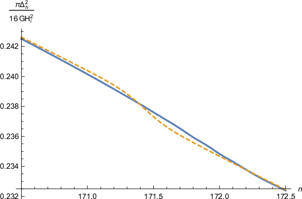
The relevant results for the tensor power spectrum are best displayed in Figure 4. The agreement between the numerically obtained exact result and our approximation (54) is almost perfect while the same is not true for the local slow-roll approximation. One hopes that in the not too far future the tensor power spectrum will be observed.
Refer to caption
Refer to caption
Figure 4: These graphs show the tensor power spectrum for the model with a feature. The left hand figure compares the exact result (solid blue) with the local slow-roll approximation (yellow dashed). The solid blue line on the right hand graph shows the logarithm of the ratio of the exact tensor power spectrum to its local slow-roll approximation. The yellow dashed line gives the non-local corrections of τ​[ϵ]​(k)\,\tau[\epsilon](k). The agreement is again excellent.

On the other hand, the scalar power spectrum signal is much stronger and has already been seen. In Figure 5 we present the results for the model of [21, 22]. There we can see the numerically obtained exact scalar power spectrum versus the local slow roll approximation (9), and versus our analytic approximation (83).

Refer to caption
Refer to caption
Figure 5: These graphs show the results for the model of Figure 3. The left hand figure compares the exact scalar power spectrum (solid blue) with its local slow-roll approximation (yellow dashed). The right hand figure compares the exact result (solid blue) with the much better approximation (yellow dashed) obtained from the full form (64), with our analytic approximation (83) for σ[ϵ](k)]\sigma[\epsilon](k)]. The local slow-roll approximation does not give a very accurate fit even to the main feature in the range  171<n<172.5\,171<n<172.5\,, and it completely misses the secondary oscillations visible in the range  172.5<n<174\,172.5<n<174. There is also a small, systematic offset before and after the features. The non-local contributions of (83) are essential for correctly reproducing the actual power spectrum.

The analytic approximation can be made even better by including the first nonlinear corrections to g⁡(n,k)g(n,k) as shown in Figure 6.

Refer to caption
Figure 6: This graph highlights the improvement made by adding the first nonlinear corrections to (83). In This figure the horizontal axis counts the number of e-foldings until the end of inflation. The most dramatic improvement is near n=172n=172.

In view of these results itt becomes evident that:
∙\bullet\; The local slow-roll approximation (9) is not accurate in reproducing the power spectrum since it only reproduces the main oscillation with quite smaller amplitude, misses all the oscillations that follow and exhibits an offset throughout.
∙\bullet\; Our analytic non-local approximation (83) accurately follows the exact power spectrum over the whole range including the “ringing” after the main oscillation.

The secondary oscillations in the scalar power spectrum are attributed to the presence of the feature which implies that ϵ′​(n)&ϵ′′​(n)≠0\epsilon^{\prime}(n)\;\&\;\epsilon^{\prime\prime}(n)\neq 0. Hence, there is deviation from the slow-roll approximation and this is imprinted in the source. Recall that the equation obeyed by the residual g⁡(n,k)g(n,k) is that of a damped driven oscillator:

g′′−Ω′Ω​g′+Ω2​g=Sgg^{\prime\prime}-\frac{\Omega^{\prime}}{\Omega}g^{\prime}+\Omega^{2}g\,=\,S_{g}\;\; (86)

The restoring force in the oscillator (86) is exponentially proportional to (−Δ​n)=−(n−nk)(-\Delta n)=-(n-n_{k}); thus:
(i) For t<tkt<t_{k} it is exponentially big and overwhelms any effect from SgS_{g}.
(ii) For t>tkt>t_{k} it is exponentially small, as is SgS_{g}, and we have no ringing.
(iii) For t≈tkt\approx t_{k} all forces are of O⁡(1)O(1) and we have the ringing from a damped driven oscillator.

In one sentence, the local slow-roll approximation cannot capture the effect of features since its only support is at tkt_{k} while a feature leads to transient tails which need non-local support and our analytic approximation provides just that.

3 From the CMBR to the Geometry

We shall now consider the inverse problem of reconstructing the geometry H⁡(n)H(n) and ϵ⁡(n)\epsilon(n) from the power spectra data Δh2​(k)\Delta^{2}_{h}(k) and Δℛ2​(k)\Delta^{2}_{\mathcal{R}}(k). Before doing so there are some remarks that must be highlighted:
∙\bullet\; It is an experimental fact that while the scalar power spectrum Δℛ2​(k)\Delta^{2}_{\mathcal{R}}(k) is very well measured, the tensor power spectrum Δh2​(k)\Delta^{2}_{h}(k) has yet to be resolved and, even when detected, it will be years before much precision is attained. Therefore, reconstruction should be based on Δℛ2​(k)\Delta^{2}_{\mathcal{R}}(k). 66 6 The tensor spectrum Δh2​(k)\Delta^{2}_{h}(k) is used only to fix the integration constant which gives the scale of inflation.
∙\bullet\; The observed smallness of ϵ⁡(n)\epsilon(n) and its assumed smoothness – up to small transients responsible for ϵ′​(n)≠0\epsilon^{\prime}(n)\neq 0 – motivates a hierarchy between HH, ϵ\epsilon and ϵ′ϵ\frac{\epsilon^{\prime}}{\epsilon} based on calculus:

H(n)=Hiexp[−∫0ndmϵ(m)],ϵ(n)=ϵiexp[∫0ndmϵ′​(m)ϵ⁡(m)].H(n)=H_{i}\,\exp\Bigl[-\!\!\int_{0}^{n}\!\!dm\;\epsilon(m)\Bigr]\quad,\quad\epsilon(n)=\epsilon_{i}\exp\Bigl[\int_{0}^{n}\!\!dm\;\frac{\epsilon^{\prime}(m)}{\epsilon(m)}\Bigr]\;\;. (87)

Hence H⁡(n)H(n) is insensitive to small errors in ϵ⁡(n)\epsilon(n), and ϵ⁡(n)\epsilon(n) is insensitive to small errors in ∂nln⁡[ϵ⁡(n)]\partial_{n}\ln[\epsilon(n)].
We will demonstrate the reconstruction algorithm by applying it to a new toy model where the scalar spectrum is made to mimic the present data by having two large features but being otherwise flat.The functional form of the scalar spectrum which we consider is:

Δℛ2​(Nk)=\displaystyle\Delta_{\mathcal{R}}^{2}(N_{k})= 19.08×10⁻⁹−9.65×10⁻¹¹​nk−1.21×10⁻⁹​e−7​(172.296−nk)2\displaystyle 19.08\times 10^{-9}-9.65\times 10^{-11}n_{k}-1.21\times 10^{-9}\,e^{-7(172.296-n_{k})^{2}} (88)
+1.18×10⁻⁹e−26​(172.85−nk)2.\displaystyle+1.18\times 10^{-9}\,e^{-26(172.85-n_{k})^{2}}\;\;.

where nkn_{k} is the number of e-foldings from the start of inflation, and inflation ends at ne=225.626n_{e}=225.626. A graph of this spectrum is shown in Figure 7. We will imagine that the tensor amplitude is Δh2​(nk=165.626)=3.1×10⁻¹¹\Delta_{h}^{2}(n_{k}=165.626)=3.1\times 10^{-11} so that HiH_{i} has the nominal value 2.8×10⁻⁵/8​π​G2.8\times 10^{-5}/\sqrt{8\pi G} at a time 60 e-foldings before the end of inflation. We stress that the exact time (or wave number) at which we fix HiH_{i} is inconsequential. In the event of a positive detection of primordial B modes we will use whichever wave number has the most well determined value for the tensor amplitude.

Refer to caption
Figure 7: The spectrum Δℛ2\Delta_{\mathcal{R}}^{2} whose geometry we will reconstruct.

* Reconstructing H⁡(n)H(n) and ϵ⁡(n)\epsilon(n):
- Step 1: The optimal variables.
It will be convenient to use dimensionless variables for our purposes by dividing out by the inflationary scale Hi≡H⁡(n=0)H_{i}\equiv H(n=0)

h⁡(n)≡H⁡(n)Hi,δ⁡(nk)≡π​Δℛ2​(k)G​Hi2,h(n)\,\equiv\,\frac{H(n)}{H_{i}}\qquad,\qquad\delta(n_{k})\,\equiv\,\frac{\pi\Delta^{2}_{\mathcal{R}}(k)}{GH_{i}^{2}}\;\;, (89)

where we recall that nkn_{k} is the number of ee-foldings from the beginning of inflation to first horizon crossing for the wave number kk.
- Step 2: The reconstruction formula.
Starting from the exact expression (64) for Δℛ2​(k)\Delta^{2}_{\mathcal{R}}(k) we note that:
(i) Because the observed first slow-roll parameter ϵ\epsilon is very small, the local slow-roll correction factor C⁡[ϵk]C[\epsilon_{k}] can be very safely ignored (see Figure 2).
(ii) Because the approximation (83) to the non-local correction exponent is superb, it can be very safely used for our purposes (see Figure 5).
Hence, expression (64) reduces to the following equation:

δ⁡(n)≃h2​(n)ϵ⁡(n)×exp⁡[∑i=15expi​(n)],\delta(n)\,\simeq\,\frac{h^{2}(n)}{\epsilon(n)}\times\exp\left[\sum_{i=1}^{5}{\rm exp}_{i}(n)\right]\;\;, (90)

which shall form the basis of our reconstruction technique. The five exponents defined in (90) are the various terms contained in (83):

exp1​(n)\displaystyle{\rm exp}_{1}(n) =\displaystyle\!\!=\!\! −∂nln[ϵ(n)]×G(1),\displaystyle-\partial_{n}\ln[\epsilon(n)]\times G(1)\;\;, (91)
exp2​(n)\displaystyle{\rm exp}_{2}(n) =\displaystyle\!\!=\!\! ∫0nd​m​∂m2ln⁡[ϵ⁡(m)]×G⁡(em−n),\displaystyle\int_{0}^{n}\!\!dm\;\partial_{m}^{2}\ln[\epsilon(m)]\times G(e^{m-n})\;\;, (92)
exp3​(n)\displaystyle{\rm exp}_{3}(n) =\displaystyle\!\!=\!\! 12​∫0nd​m​[∂mln⁡[ϵ⁡(m)]]2×G⁡(em−n),\displaystyle\frac{1}{2}\!\int_{0}^{n}\!\!dm\;\Big[\partial_{m}\ln[\epsilon(m)]\Big]^{2}\times G(e^{m-n})\;\;, (93)
exp4​(n)\displaystyle{\rm exp}_{4}(n) =\displaystyle\!\!=\!\! ∫0nd​m​∂mln⁡[ϵ⁡(m)]×G⁡(em−n),\displaystyle 3\!\int_{0}^{n}\!\!dm\;\partial_{m}\ln[\epsilon(m)]\times G(e^{m-n})\;\;, (94)
exp5​(n)\displaystyle{\rm exp}_{5}(n) =\displaystyle\!\!=\!\! ∫n∞d​m​∂mln⁡[ϵ⁡(m)]×G⁡(em−n)1+e2​(m−n).\displaystyle 2\!\int_{n}^{\infty}\!\!dm\;\partial_{m}\ln[\epsilon(m)]\times\frac{G(e^{m-n})}{1+e^{2(m-n)}}\;\;. (95)

- Step 3: Reconstructing H⁡(n)H(n).
The reconstruction of the Hubble parameter is quite simple. We ignore all the exponents in the relevant equation (90) and only keep the leading slow-roll terms:

δ⁡(n)≃h2​(n)ϵ⁡(n)⟹h2​(n)≃1+∫0ndm2δ⁡(m).\delta(n)\,\simeq\,\frac{h^{2}(n)}{\epsilon(n)}\quad\Longrightarrow\quad h^{2}(n)\,\simeq\,\frac{1}{1\!+\!\int_{0}^{n}\!dm\;\frac{2}{\delta(m)}}\;\;. (96)

Applying (96) yields results which are excellent for fitting the flat parts of the spectrum. This interpolation is limited however since it does not contain any of the nonlocal character of the scalar spectrum and hence will not reproduce the features in the spectrum (88). We will construct an even better interpolation of h⁡(n)h(n) at the end when we integrate our reconstructed ϵ⁡(n)\epsilon(n) according to equation (87).
- Step 3: Reconstructing ϵ⁡(n)\epsilon(n).
The case of the reconstruction of ϵ⁡(n)\epsilon(n) is much more delicate. We start by noting that in general {exp1(n)\{{\rm exp}_{1}(n), exp2​(n){\rm exp}_{2}(n) and exp4(n)}{\rm exp}_{4}(n)\} are much larger than {exp3(n)\{{\rm exp}_{3}(n) and exp5(n)}{\rm exp}_{5}(n)\} for models with transient features like the ones under consideration. The reason for this is that any deviations from slow roll which make exp3​(n){\rm exp}_{3}(n) large will necessarily make the other terms exp2​(n){\rm exp}_{2}(n) and exp4​(n){\rm exp}_{4}(n) even larger by about an order of magnitude [11]. Moreover, as can be seen in (95) the term exp5{\rm exp}_{5}(n) is supressed relative to the other terms by the factor (1+e2​(m−n))−1(1+e^{2(m-n)})^{-1} in the integrand. These important facts make the optimal distribution of the five exponents in (90) transparent; upon taking the logarithm we get:

−ln⁡[ϵ⁡(n)]−exp1⁡(n)−exp2⁡(n)−exp4⁡(n)\displaystyle-\ln[\epsilon(n)]-{\rm\exp}_{1}(n)-{\rm\exp}_{2}(n)-{\rm\exp}_{4}(n) ≃\displaystyle\!\!\simeq\!\! (97)
−ln⁡[δ⁡(n)]+2​ln⁡[h⁡(n)]+exp3⁡(n)+exp5⁡(n).\displaystyle\hskip-110.96556pt-\ln[\delta(n)]+2\ln[h(n)]+{\rm\exp}_{3}(n)+{\rm\exp}_{5}(n)\;\;.\qquad

It should be apparent that we cannot solve (97) exactly and we must develop an approximation technique. One such technique is an iterative procedure with the following reconstruction logic:
∙\bullet\; We define the source 𝒮ϵ​(n){\cal S}_{\epsilon}(n) as:

𝒮ϵ​(n)≡−ln⁡[δ⁡(n)]+2​ln⁡[h⁡(n)]+exp3⁡(n)+exp5⁡(n).{\cal S}_{\epsilon}(n)\,\equiv\,-\ln[\delta(n)]+2\ln[h(n)]+{\rm\exp}_{3}(n)+{\rm\exp}_{5}(n)\;\;. (98)

The first term in (98) is determined from the measured primordial spectrum which gives δ⁡(n)\delta(n).
∙\bullet\; As the lowest order source that can provide a lowest order solution we can take:

𝒮0​(n)≡−ln⁡[δ⁡(n)]−ln⁡[1+∫0nd​m​2δ⁡(m)].{\cal S}_{0}(n)\,\equiv\,-\ln[\delta(n)]-\ln\left[1+\int_{0}^{n}\!\!dm\;\frac{2}{\delta(m)}\right]\;\;. (99)

Here we have determined the second term in (98) from the slow-roll formula (96) which gives h⁡(n)h(n) in terms of δ⁡(n)\delta(n); a decent approximation because the Hubble parameter does not change much due to the presence of the feature. We have also ignored the two weak terms exp3​(n){\rm exp}_{3}(n) and exp5​(n){\rm exp}_{5}(n).
∙\bullet\; The resulting lowest order equation:

[1+G(1)∂n]ln[ϵ(n)]−∫0ndm[∂m2+3∂m]ln[ϵ(m)]×G(em−n)≃𝒮0(n),\Big[1+G(1)\partial_{n}\Big]\ln[\epsilon(n)]-\int_{0}^{n}\!\!dm\;\Big[\partial_{m}^{2}+3\partial_{m}\Big]\ln[\epsilon(m)]\times G(e^{m-n})\,\simeq\,{\cal S}_{0}(n)\;\;, (100)

is a linear non-local equation that can be solved by the Green’s function method:

ln⁡[ϵ⁡(n)]=∫0∞d​m​𝒢​(n−m)×𝒮0​(m),\ln[\epsilon(n)]=\int_{0}^{\infty}\!dm\;\mathcal{G}(n\!-\!m)\times{\cal S}_{0}(m)\;\;, (101)

where the Green’s function 𝒢⁡(n)\mathcal{G}(n) is the solution to (100) for a delta function source: 77 7 The function 𝒢\mathcal{G} becomes symmetric in its arguments because the function G⁡(en−nk)G(e^{n-n_{k}}) given by (37) is essentially zero for the interval up to N∼4N\sim 4 ee-foldings before first horizon crossing.

[1+G(1)∂n]𝒢(n)−∫−Nndm[∂m2+3∂m]𝒢(m)×G(em−n)=δ(n).\Big[1+G(1)\partial_{n}\Big]\mathcal{G}(n)-\int_{-N}^{n}\!\!dm\;\Big[\partial_{m}^{2}+3\partial_{m}\Big]\mathcal{G}(m)\times G(e^{m-n})\,=\,\delta(n)\;\;. (102)

The presence of the function G⁡(en−nk)G(e^{n-n_{k}}) in (102) makes solving exactly for 𝒢⁡(n)\mathcal{G}(n) elusive. For the sake of simplicity it is easier to approach this problem after taking a Laplace transform because this turns our integro-differntial equation into an algebraic one. In the Laplace domain the Green’s function equation we wish to solve is:

[+G⁡(1)​s−(s+3)​s×ℐ⁡(s)]​𝒢^​(s,m)=e−m​s,\Bigl[1\!+\!G(1)s\!-\!(s\!+\!3)s\!\times\!\mathcal{I}(s)\Bigr]\widehat{\mathcal{G}}(s;m)=e^{-ms}\;, (103)

where 𝒢^​(s,m)\widehat{\mathcal{G}}(s;m) is the retarded Green’s function we wish to find and we have defined,

ℐ⁡(s)≡∫0∞d​ℓ​e−s​ℓ×G⁡(e−ℓ).\mathcal{I}(s)\equiv\int_{0}^{\infty}\!\!d\ell\,e^{-s\ell}\!\times\!G(e^{-\ell})\;. (104)

We have show previously that a very good approximation for ℐ⁡(s)\mathcal{I}(s) is given by:

ℐ⁡(s)=ℐ0​(s)+ℐ1​(s)\displaystyle\mathcal{I}(s)=\mathcal{I}_{0}(s)+\mathcal{I}_{1}(s) (105)
ℐ0​(s)=G⁡(1)s​[1−e−0.8​s]\displaystyle\mathcal{I}_{0}(s)=\frac{G(1)}{s}\Bigl[1-e^{-0.8s}\Bigr] (106)
ℐ1​(s)=0.154(s+8.97)2​sin⁡[1.76​(−e−0.262​(s−3.78))]\displaystyle\mathcal{I}_{1}(s)=\frac{0.154}{(s+8.97)^{2}}\,\sin\Biggl[1.76\Bigl(1\!-\!e^{-0.262(s-3.78)}\Bigr)\Biggr] (107)

for real values of ss [11]. Since finding the proper inverse transform is rather complicated, we simplify the process by expanding ℐ⁡(s)\mathcal{I}(s) into its Taylor series. The solution for 𝒢^\widehat{\mathcal{G}} is then expanded as a geometric series and the inverse transform is done term by term using the identity:

ℒ−1​[e−a×s(s+b)q]=e−b⁡(a+n)​Θ​(a+n)×(a+n)q−1Γ⁡(n)\mathcal{L}^{-1}\left[\frac{e^{-a\times s}}{(s+b)^{q}}\right]=\frac{e^{-b(a+n)}\Theta\left(a+n\right)\times\left(a+n\right)^{q-1}}{\Gamma(n)} (108)

The results for reconstructing the geometry of our mock spectrum are show in Figure 8.

Refer to caption
Refer to caption
Figure 8: The left hand graph shows the values of ln⁡[ϵ⁡(n)]\ln\left[\epsilon(n)\right] which we have reconstructed from (88). On the right hand side are the two different interpolations of the Hubble parameter H⁡(n)H(n). The orange curve is the result of integrating ϵ⁡(n)\epsilon(n) according to 2 while the blue dashed curve comes from the leading slow roll terms in (96). Note that the curves agree on the edges of the figure but disagree near the feature.

What we have found is that in order to produce a spectrum with exactly two features one would require two features in the geometry as opposed to the usual case where only one is considered. The first peak induces the ringing in the system just like we see in the step model however in this case the slight dip after the peak has the effect of canceling out the secondary peaks. We perform a check of our reconstruction by integrating ϵ0​(n)\epsilon_{0}(n) to obtain a new value of H⁡(n)H(n) and then inserting both into equation (64) and comparing with our original model. This can be seen in Figure 9 and the results speak for themselves.

Refer to caption
Figure 9: The spectrum from the reconstructed geometry of Figure 8 compared with the mock spectrum we started with.

We must stress that what we have done here is truely novel. We have not proposed any analytic model for either the potential or the geometry. We have explicitly constructed an excellent approximation to the geometry which would produce a model spectrum which mimics current data.

4 Epilogue

In this paper we have presented a formalism that is applicable to geometries that include the presence of non-trivial features in their history. The formalism enables us to obtain analytic expressions for the primordial power spectra and also reconstruct the geometry given the power spectra as input.

The formalism determines the tree order power spectra by evolving the norm-squared mode functions. Even if considered purely as a numerical technique this is more efficient than evolving the mode functions because it avoids keeping track of the rapidly fluctuating phase, and because it converges about twice as fast. Moreover, the formalism applies not only to single-scalar inflation but also to any conformally related model, such as f⁡(R)f(R) inflation [23] and Higgs inflation, whose power spectra are numerically identical.

The methodology breaks down if the first slow-roll parameter ϵ\epsilon becomes big, or if the non-linear terms in the evolution equations become big. The power spectra results presented show that:
(i) The slow-roll approximation breaks down when the geometry contains non-trivial features.
(ii) The non-local correction exponents τ⁡[ϵ]\tau[\epsilon] and σ⁡[ϵ]\sigma[\epsilon] are essential in reaching quantitative accuracy.

In reconstructing the geometry from the power spectra data, our results indicate that further improvement is needed for the accurately handling of derivatives of the first slow-roll parameter ϵ\epsilon; as far as the undifferentiated ϵ\epsilon is concerned our errors are accurate within ±2.2%\pm 2.2\% and for the Hubble parameter they never exceed 0.04%0.04\%. These results seem to improve on other techniques [24, 25, 26].

Another application concerns improving the classic consistency relation [27, 28, 29] for comparing the tensor power spectrum (when it is finally resolved) with its well-measured scalar counterpart to test single-scalar inflation. We have proposed a modification [30] which:
(i) Avoids the need to take a derivative of Δh2​(k)\Delta^{2}_{h}(k) that would degrade the accuracy of the poorly resolved initial detections.
(ii) Integrates the high quality data we already possess for Δℛ2​(k)\Delta^{2}_{\mathcal{R}}(k).
(iii) Can be used to cross-correlate scalar features (e.g., Fig. 5) with the tensor features (e.g., Fig. 4), in the far future, when both spectra are well resolved.

A particularly exciting application of our formalism is to exploit the control it gives over how the mode functions depend upon ϵ⁡(n)\epsilon(n) to design a new statistic to cross-correlate features in the power spectrum with non-Gaussianity. This has already been proposed in the context of models with variable speed of sound [31, 32], and developed numerically [33], but it can now be done analytically for simple scalar potential models. The idea is that non-Gaussianity measures self-interaction, which is what a step in the potential provides. There may be an observable effect which is not resolvable by generic statistics but could be detected by a precision search.

Finally, we mention using the formalism to motivate better phenomenological models [34] of the late time regime of Λ\Lambda-driven inflation [35, 36]. The fundamental assumption is that quantum gravitational back-reaction grows like the coincidence limit of the tensor propagator, which can be expressed as an integral of M⁡(t,k)M(t,k) [37]. Inferring how this quantity depends on a general geometry defines the model.

Acknowledgements

This work was partially supported by the European Union’s Horizon 2020 Programme under grant agreement 669288-SM-GRAV-ERC-2014-ADG; by NSF grant PHY-1506513; and by the Institute for Fundamental Theory at the University of Florida.

References

  • [1] A. A. Starobinsky, JETP Lett. 30, 682 (1979) [Pisma Zh. Eksp. Teor. Fiz. 30, 719 (1979)].
  • [2] V. F. Mukhanov and G. V. Chibisov, JETP Lett. 33, 532 (1981) [Pisma Zh. Eksp. Teor. Fiz. 33, 549 (1981)].
  • [3] V. F. Mukhanov, H. A. Feldman and R. H. Brandenberger, Phys. Rept. 215, 203 (1992). doi:10.1016/0370-1573(92)90044-Z
  • [4] A. R. Liddle and D. H. Lyth, Phys. Rept. 231, 1 (1993) doi:10.1016/0370-1573(93)90114-S [astro-ph/9303019].
  • [5] J. E. Lidsey, A. R. Liddle, E. W. Kolb, E. J. Copeland, T. Barreiro and M. Abney, Rev. Mod. Phys. 69, 373 (1997) doi:10.1103/RevModPhys.69.373 [astro-ph/9508078].
  • [6] R. P. Woodard, Int. J. Mod. Phys. D 23, no. 09, 1430020 (2014) doi:10.1142/S0218271814300201 [arXiv:1407.4748 [gr-qc]].
  • [7] P. A. R. Ade et al. [Planck Collaboration], Astron. Astrophys. 594, A20 (2016) doi:10.1051/0004-6361/201525898 [arXiv:1502.02114 [astro-ph.CO]].
  • [8] A. A. Starobinsky, JETP Lett. 55, 489 (1992) [Pisma Zh. Eksp. Teor. Fiz. 55, 477 (1992)].
  • [9] L. M. Wang, V. F. Mukhanov and P. J. Steinhardt, Phys. Lett. B 414, 18 (1997) doi:10.1016/S0370-2693(97)01166-0 [astro-ph/9709032].
  • [10] P. A. R. Ade et al. [Planck Collaboration], Astron. Astrophys. 594, A13 (2016) doi:10.1051/0004-6361/201525830 [arXiv:1502.01589 [astro-ph.CO]].
  • [11] D. J. Brooker, N. C. Tsamis and R. P. Woodard, Phys. Rev. D 96, no. 10, 103531 (2017) doi:10.1103/PhysRevD.96.103531 [arXiv:1708.03253 [gr-qc]].
  • [12] S. P. Miao and R. P. Woodard, JCAP 1207, 008 (2012) doi:10.1088/1475-7516/2012/07/008 [arXiv:1204.1784 [astro-ph.CO]].
  • [13] M. G. Romania, N. C. Tsamis and R. P. Woodard, JCAP 1208, 029 (2012) doi:10.1088/1475-7516/2012/08/029 [arXiv:1207.3227 [astro-ph.CO]].
  • [14] D. J. Brooker, N. C. Tsamis and R. P. Woodard, Phys. Rev. D 93, no. 4, 043503 (2016) doi:10.1103/PhysRevD.93.043503 [arXiv:1507.07452 [astro-ph.CO]].
  • [15] D. J. Brooker, N. C. Tsamis and R. P. Woodard, Phys. Rev. D 94, no. 4, 044020 (2016) doi:10.1103/PhysRevD.94.044020 [arXiv:1605.02729 [gr-qc]].
  • [16] L. Covi, J. Hamann, A. Melchiorri, A. Slosar and I. Sorbera, Phys. Rev. D 74, 083509 (2006) doi:10.1103/PhysRevD.74.083509 [astro-ph/0606452].
  • [17] J. Hamann, L. Covi, A. Melchiorri and A. Slosar, Phys. Rev. D 76, 023503 (2007) doi:10.1103/PhysRevD.76.023503 [astro-ph/0701380].
  • [18] D. K. Hazra, M. Aich, R. K. Jain, L. Sriramkumar and T. Souradeep, JCAP 1010, 008 (2010) doi:10.1088/1475-7516/2010/10/008 [arXiv:1005.2175 [astro-ph.CO]].
  • [19] D. K. Hazra, A. Shafieloo, G. F. Smoot and A. A. Starobinsky, JCAP 1408, 048 (2014) doi:10.1088/1475-7516/2014/08/048 [arXiv:1405.2012 [astro-ph.CO]].
  • [20] D. K. Hazra, A. Shafieloo, G. F. Smoot and A. A. Starobinsky, JCAP 1609, no. 09, 009 (2016) doi:10.1088/1475-7516/2016/09/009 [arXiv:1605.02106 [astro-ph.CO]].
  • [21] M. J. Mortonson, C. Dvorkin, H. V. Peiris and W. Hu, Phys. Rev. D 79, 103519 (2009) doi:10.1103/PhysRevD.79.103519 [arXiv:0903.4920 [astro-ph.CO]].
  • [22] J. A. Adams, B. Cresswell and R. Easther, Phys. Rev. D 64, 123514 (2001) doi:10.1103/PhysRevD.64.123514 [astro-ph/0102236].
  • [23] D. J. Brooker, S. D. Odintsov and R. P. Woodard, Nucl. Phys. B 911, 318 (2016) doi:10.1016/j.nuclphysb.2016.08.010 [arXiv:1606.05879 [gr-qc]].
  • [24] K. Kadota, S. Dodelson, W. Hu and E. D. Stewart, Phys. Rev. D 72, 023510 (2005) doi:10.1103/PhysRevD.72.023510 [astro-ph/0505158].
  • [25] J. D. Barrow and A. Paliathanasis, arXiv:1611.06680 [gr-qc].
  • [26] J. Mastache, F. Zago and A. Kosowsky, Phys. Rev. D 95, no. 6, 063511 (2017) doi:10.1103/PhysRevD.95.063511 [arXiv:1611.03957 [astro-ph.CO]].
  • [27] D. Polarski and A. A. Starobinsky, Phys. Lett. B 356, 196 (1995) doi:10.1016/0370-2693(95)00842-9 [astro-ph/9505125].
  • [28] J. Garcia-Bellido and D. Wands, Phys. Rev. D 52, 6739 (1995) doi:10.1103/PhysRevD.52.6739 [gr-qc/9506050].
  • [29] M. Sasaki and E. D. Stewart, Prog. Theor. Phys. 95, 71 (1996) doi:10.1143/PTP.95.71 [astro-ph/9507001].
  • [30] D. J. Brooker, N. C. Tsamis and R. P. Woodard, Phys. Lett. B 773, 225 (2017) doi:10.1016/j.physletb.2017.08.027 [arXiv:1603.06399 [astro-ph.CO]].
  • [31] A. Ach�carro, J. O. Gong, G. A. Palma and S. P. Patil, Phys. Rev. D 87, no. 12, 121301 (2013) doi:10.1103/PhysRevD.87.121301 [arXiv:1211.5619 [astro-ph.CO]].
  • [32] J. Torrado, B. Hu and A. Achucarro, Phys. Rev. D 96, no. 8, 083515 (2017) doi:10.1103/PhysRevD.96.083515 [arXiv:1611.10350 [astro-ph.CO]].
  • [33] D. K. Hazra, L. Sriramkumar and J. Martin, JCAP 1305, 026 (2013) doi:10.1088/1475-7516/2013/05/026 [arXiv:1201.0926 [astro-ph.CO]].
  • [34] N. C. Tsamis and R. P. Woodard, JCAP 1409, 008 (2014) doi:10.1088/1475-7516/2014/09/008 [arXiv:1405.4470 [astro-ph.CO]].
  • [35] N. C. Tsamis and R. P. Woodard, Int. J. Mod. Phys. D 20, 2847 (2011) doi:10.1142/S0218271811020652 [arXiv:1103.5134 [gr-qc]].
  • [36] N. C. Tsamis and R. P. Woodard, Nucl. Phys. B 474, 235 (1996) doi:10.1016/0550-3213(96)00246-5 [hep-ph/9602315].
  • [37] M. G. Romania, N. C. Tsamis and R. P. Woodard, Lect. Notes Phys. 863, 375 (2013) doi:10.1007/978-3-642-33036-0_13 [arXiv:1204.6558 [gr-qc]].