Progressive Bit-Flipping Decoding of Polar Codes Over Layered Critical Sets

We use $a_{1}^{N}$ to denote a vector $(a_{1},a_{2},...,a_{N})$. For polar codes with block-length $N=2^{n}$ and kernel $\tiny{\bm{G}_{2}=\begin{bmatrix}1\;0\\ 1\;1\end{bmatrix}}$, we denote $u_{1}^{N}$ as the information sequence, and a polar codeword $c_{1}^{N}$ is obtained by $c_{1}^{N}=u_{1}^{N}\bm{B}_{N}\bm{G}_{2}^{\otimes n}$, where ‘$\otimes$’ denotes the Kronecker product while $\bm{B}_{N}$ is a permutation matrix. A coding rate $R=K/N$ means that a set $\mathcal{A}\subset\{1,2,...,N\}$ of cardinality $K$ is selected as the information set (see [1]), and thus $u_{1}^{N}$ consists of $K$ unfrozen bits and $N-K$ frozen bits (all frozen bits are assumed to be zero if not specified). The split channel is defined as $W_{N}^{(i)}(y_{1}^{N},u_{1}^{i-1}|u_{i})=\sum_{u_{i+1}^{N}\in\mathcal{X}^{N-i}}\frac{1}{2^{N-1}}W_{N}(y_{1}^{N}|u_{1}^{N})$, and the Bhattacharyya parameter $Z(W_{N}^{(i)})$ is computed to select the $K$ most reliable split channels to transmit unfrozen bits. Interested readers are referred to [1] for more details.

The framework in [9] is adopted for the ensuing analysis. To facilitate understanding, let us consider a toy example of polar codes with block-length $N=2^{2}$ and information sequence $u_{1}^{4}=\left(u_{1},u_{2},u_{3},u_{4}\right)$. $u_{3}$ and $u_{4}$ are chosen as the unfrozen bits, thus inducing a coding rate $R=2/4$.

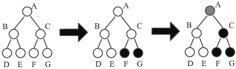
To proceed, a full binary tree with $N=2^{2}$ leaf nodes is constructed in Fig. 1 (left). The leaf nodes $\{D,E,F,G\}$ correspond to the information bits $\{u_{1},u_{2},u_{3},u_{4}\}$, respectively. Since $u_{3}$ and $u_{4}$ are unfrozen bits, nodes $F$ and $G$ are denoted by black circles for the sake of clarity, see Fig. 1 (middle) for illustration. Furthermore, for each non-leaf node in the tree, if its two descendants are of the same color, then it is marked with that color as well. Otherwise, it is indicated by a gray circle. This process starts from the bottom non-leaf nodes until the root node is reached, as shown in Fig. 1 (right).

To implement polar encoding, a constituent code is assigned to each node in Fig. 1 (right). Suppose that $u_{1}^{4}=(0,0,1,0)$, i.e., $D[1]=0$, $E[1]=0$, $F[1]=1$, $G[1]=0$, where $D[i]$ denotes the $i$-th component at node $D$. On this basis, the constituent code at node $B$ is obtained by $(B[1],B[2])=(D[1],E[1])\times\bm{G}_{2}$, which gives $B[1]=B[2]=0$. Similarly, we have $C[1]=1$ and $C[2]=0$. Next, invoking the expressions $(A[1],A[2])=(B[1],C[1])\times\bm{G}_{2}$ and $(A[3],A[4])=(B[2],C[2])\times\bm{G}_{2}$, the polar codeword is obtained as $c_{1}^{4}=(A[1],A[2],A[3],A[4])=(1,1,0,0)$. One can also check that $c_{1}^{4}$ can be obtained by $c_{1}^{4}=(D[1],E[1],F[1],G[1])\times\bm{B}_{4}\bm{G}_{2}^{\otimes 2}$. As for SC decoding, it starts from the root node $A$, which possesses the LLRs received from the underlying channel, and uses[1, Eq. 75] and [1, Eq. 76] to calculate LLRs recursively. In the meantime, polarization can also be interpreted based on this tree. One can check that node $A$ has four independent copies of the underlying channel $W$, while node $B$ has two independent copies of the synthetic channel $W_{2}^{(1)}$ and node $C$ has two independent copies of the synthetic channel $W_{2}^{(2)}$. Finally, a leaf node has a unique copy of the split channel, e.g., node $E$ has $W_{4}^{(2)}$. We refer the reader to [9] for more details. It is worth noting that this framework can be extended to polar codes with arbitrary block-length.

Let us focus on a more complicated example as shown in Fig. 2, where $N=2^{4}$ and $K=9$ (the information set may not be reasonable).

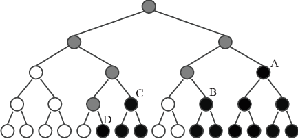
In our framework, SC decoding is not viewed as a bit-by-bit process, but from a subblock-by-subblock perspective. Once the full binary tree corresponding to the current specific polar code is constructed, the entire polar code is divided into multiple sub-polar codes (also called subblocks), which all have coding rate $R=1$. In Fig. 2, there exist four such subblocks, which are denoted by the corresponding root nodes $A$, $B$, $C$ and $D$, respectively (they are also polar codes but with shorter block-length). The subblock consists of only unfrozen bits, e.g, node $A$ has unfrozen bits $u_{13}^{16}$. In particular, node $D$ has an unfrozen bit $u_{6}$, and it can be viewed as a special subblock which has itself as both the codeword (root node) and information sequence (leaf node).

Now, consider a general subblock $A$ ($A$ denotes its root node) which has $M=2^{m}$ unfrozen bits. We use $u_{1}^{M}$ and $c_{1}^{M}$ to denote its information sequence and codeword, respectively. Then the following proposition is derived, which sheds light on our main results.

Capitalizing on the results above, there is a high probability that the first incorrectly estimated unfrozen bit happens to be the first unfrozen bit within the subblock. Inspired by this, we provide a method to construct a set $S$ that almost surely includes the first incorrect hard decision in SC decoding. The corresponding algorithm is summarized as Algorithm 1.

Taking Fig. 2 for instance, we have $S=\{u_{6},u_{7},u_{11},u_{13}\}$. Note that the number of elements in set $S$ is exactly the same as that of subblocks, which is rather small compared with the information set $\mathcal{A}$ of cardinality $K$. Furthermore, $S$ is uniquely determined once the construction of polar codes is completed.

To validate the above method, we first focus on the evaluation of the difference $P_{\text{s\_bler}}-P_{u_{1}}$. To the best of our knowledge, the exact values of $P_{\text{s\_bler}}$ and $P_{u_{1}}$ are rather difficult to compute. Thereby, we exploit the Gaussian approximation method to provide some insightful results. Gaussian approximation was introduced in [10] and adopted for the analysis of polar codes in [11]. In the following analysis, we restrict our attention to binary phase shift keying (BPSK) modulation, i.e., for a given AWGN channel, the received symbol is expressed as $y_{i}=x_{i}+n_{i}$, where $x_{i}=1-2c_{i}$, and $n_{i}$ represents a Gaussian random variable with mean zero and variance $\sigma^{2}$. Without loss of generality, we assume that the all-zero codeword is transmitted. In this sense, one can check that the received LLR can be written as $L(y_{i})=\mathrm{log}\frac{W(y_{i}|x_{i}=1)}{W(y_{i}|x_{i}=-1)}=\frac{2y_{i}}{\sigma^{2}}$, which can be viewed as a Gaussian random variable with mean $\frac{2}{\sigma^{2}}$ and variance $\frac{4}{\sigma^{2}}$. By rewriting formulae [1, Eq.75] and [1, Eq.76] in an LLR form, one can find that the operations involved in SC decoding are exactly the same as those in belief propagation decoding. Thus, as suggested in [10], by assuming that the symmetry condition is always satisfied, all the LLRs involved in SC decoding can be viewed as Gaussian random variables with the form $\mathcal{N}(\mu,2\mu)$. We only need to calculate the mean $\mu$.

For a given subblock $A$, suppose that the LLR corresponding to the synthetic channel $W_{M}$ satisfies $\mathcal{N}(\mu,2\mu)$. Then the LLR corresponding to the split channel $W_{M}^{(1)}$ takes a mean $\mu_{u_{1}}=\phi^{-1}(1-\big(1-\phi(\mu)\big)^{2^{m}})$, where $\phi(x)$ is defined as

Due to the all-zero codeword, the probability that $u_{1}$ is incorrectly estimated is calculated as $P_{u_{1}}=Q(\sqrt{\mu_{u_{1}}/2})$, where $Q(x)=\frac{1}{\sqrt{2\pi}}\int_{x}^{+\infty}e^{-\frac{t^{2}}{2}}dt$. Similarly, the error probability of the entire subblock is $P_{\text{s\_bler}}=1-(1-Q(\sqrt{\mu/2}))^{2^{m}}$.

The numerical comparison between $P_{\text{s\_bler}}$ and $P_{u_{1}}$ using Gaussian approximation is depicted in Fig. 3. It can be observed that for large length $M$ and small $\mu$, there still exists some obvious difference between $P_{\text{s\_bler}}$ and $P_{u_{1}}$. This is practical because, firstly, small $\mu$ means that the synthetic channel $W_{M}$ is not quite reliable, and thus it is more likely to introduce more than one error; secondly, large $M$ increases the probability to include two or more errors as well. Thus, the difference $P_{\text{s\_bler}}-P_{u_{1}}=\sum_{i=1}^{M/2}C_{M}^{2i}p^{2i}(1-p)^{M-2i}$ becomes noticeable. However, we conjecture that for any given underlying channel $W$ to implement polarization, a subblock $A$ with large $M$ in general has a large $\mu$ as well. For larger $M$, the split channel $W_{M}^{(1)}$ is further degraded compared with the synthetic channel $W_{M}$. As $W_{M}^{(1)}$ is selected to transmit an unfrozen bit, thus $W_{M}$ should be sufficiently reliable as well, since otherwise $u_{1}$ will turn into a frozen bit. It can be seen in Fig. 3 that if $\mu$ is large enough, the difference between $P_{\text{s\_bler}}$ and $P_{u_{1}}$ can usually be neglected.

To further evaluate the Algorithm 1, we focus on the probability that the first incorrect hard decision falls into set $S$ through Monte Carlo simulations, which is shown in Table I. The “Included in set $S$” denotes the number that the first incorrectly estimated unfrozen bit falls into the critical set $S$, and “Incorrect blocks” denotes the total number of blocks that are not correctly recovered, while “Accuracy” simply computes their ratio. It can be observed that the probability that the first error is included in the critical set $S$ approaches $100\%$, even for low signal to noise ratios (SNRs). Furthermore, the performance of Algorithm 1 improves as SNR increases, which is consistent with our prior analysis.

Now suppose that $\hat{u}_{i}$ is the first incorrect hard decision and is flipped to $1-\hat{u}_{i}$ based on the bit-flipping method. Under this condition, all the elements in $u_{1}^{i}$ can be viewed as frozen bits. The reason is that, for the split channel $W_{N}^{(i+1)}(y_{1}^{N},u_{1}^{i}|u_{i+1})$, the estimate of $u_{i+1}$ is determined once the sequence $\hat{u}_{1}^{i}$ is provided. And therefore, whether some $u_{j}$ with $1\leq j\leq i$ is a frozen bit or unfrozen bit no longer makes any difference.

By considering $\{u_{1},\cdots,u_{i}\}$ as frozen bits, a new full binary tree similar to Fig. 2 can be established immediately. However, at this time, all nodes corresponding to $u_{1}^{i}$ are white nodes, while the colors of the following nodes corresponding to $u_{i+1}^{N}$ still depend on whether it is a frozen bit or unfrozen bit. Based on this new tree, we can construct a modified critical set $S^{\prime}$ using Algorithm 1. This modified critical set implies that if errors occur in estimating $u_{i+1}^{N}$ under SC decoding, the first incorrect hard decision should be almost surely included in such a set. By adopting the bit-flipping operation as done for $u_{i}$, this error is promised to be corrected, thus further improving the performance. Note that, including $u_{i}$, the above scheme has corrected two errors during SC decoding.

Interestingly, this scheme can be extended to correct more errors based on a tree structure. Taking the polar code in Fig. 2 for example, the tree structure based implementation of progressive bit-flipping decoding is depicted in Fig. 4, where each node denotes an estimate of $u_{1}^{N}$ as a candidate sequence and the edge indicates the unfrozen bit that is flipped. The tree is built via the following steps: first, conventional SC decoding is employed to obtain the root node at level $0$, which denotes the candidate sequence $\hat{u}_{1}^{N}$ without flipping any bits; next, the critical set $S_{1}=\{u_{6},u_{7},u_{11},u_{13}\}$ is constructed to obtain nodes at level $1$, i.e., every unfrozen bit in $S_{1}$ corresponds to an edge extended from the root node; then, for each node at level $1$, e.g., node $E$, it constructs a modified critical set $S^{\prime}=\{u_{14},u_{15}\}$ by building a full binary tree similar to Fig. 2, with the leaf nodes corresponding to $u_{1}^{13}$ being white and those corresponding to $u_{14}^{16}$ being black, thus inducing the edges and nodes at level $2$. Intuitively, repeating the steps above gives rise to the following levels of the tree.

On the basis of such tree structure, the bit-flipping decoding scheme is implemented in a level-order traversal, starting from the root node. In particular, for each node, the entire edges that start from the root node constitute the unfrozen bits that should be flipped. For instance, the node $F$ in Fig. 4 means that: SC decoding is first implemented to compute $\hat{u}_{1}^{13}$, but $\hat{u}_{13}$ is flipped; then SC decoding is continued to compute $\hat{u}_{14}^{15}$, but $\hat{u}_{15}$ is flipped as well; finally SC decoding is implemented to compute $\hat{u}_{16}$ and thus a candidate sequence $\hat{u}_{1}^{16}$ is obtained at this node. The “level” in fact indicates the number of unfrozen bits that are flipped, and specifically level $0$ denotes the conventional SC decoding without flipping any unfrozen bits. Therefore, the progressive bit-flipping decoding can be viewed as a tree search process.

To further reduce the search complexity, the current node should not generate any child node if it contains some incorrectly flipped unfrozen bits. According to Gaussian approximation, if all the prior flipped unfrozen bits are correct, the LLRs at $u_{i}^{N}$ should not be too small compared with their mean values. Based on this observation, we can assign a threshold $\omega_{l}$ to the $l$-th level in the tree structure, and design a metric $\mu_{i}-\gamma_{\text{left}}\sigma_{i}$, where $\sigma_{i}=\sqrt{2\mu_{i}}$ and $\gamma_{\text{left}}$ is an optimized value derived through numerical simulations. By counting the number of unfrozen bits in $u_{i}^{N}$ as $N_{1}$, while the number of unfrozen bits whose LLRs fail in achieving $\mu_{i}-\gamma_{\text{left}}\sigma_{i}$ as $N_{2}$ (note that unfrozen bits belonging to the critical set are excluded when counting $N_{1}$ and $N_{2}$), we define $E_{\textrm{NoChild}}$ as the event $\frac{N_{2}}{N_{1}}>=\omega_{l}$, if $E_{\textrm{NoChild}}$ is true, then the estimate sequence $\hat{u}_{1}^{i-1}$ is supposed to contain at least one error, thus the branches extended from the current node can be pruned. Otherwise, the current node is allowed to generate child nodes.

If the current node is determined to generate its child nodes, then the unfrozen bits which are likely to be correct should not be selected as child nodes. Recall that under Gaussian approximation, given that $\hat{u}_{1}^{i-1}=u_{1}^{i-1}$, if $\textrm{LLR}(u_{i})$ is larger than its mean value, then $u_{i}$ is supposed to be correct. On this basis, we design a threshold $\mu_{i}+\gamma_{\text{right}}\sigma_{i}$, where $\sigma_{i}=\sqrt{2\mu_{i}}$ and $\gamma_{\text{right}}$ is a constant. We define $E_{\textrm{NotSelect}}(u_{i})$ as the event $L(u_{i})>\mu_{i}+\gamma_{\text{right}}\sigma_{i}$, if event $E_{\textrm{NotSelect}}(u_{i})$ is true, then $u_{i}$ is not selected to be the child node.

The proposed progressive multi-level bit-flipping decoding algorithm using the above pruning rules is summarized as Algorithm 2, where $S_{l}$ denotes the set of unfrozen bits that should be flipped at level $l$.

References

- [1] E. Arıkan, “Channel polarization: A method for constructing capacity-achieving codes for symmetric binary-input memoryless channels,” IEEE Trans. Inf. Theory, vol. 55, no. 7, pp. 3051-3073, Jul. 2009.
- [2] Chairman¡¯s notes, 3GPP TSG RAN WG1 , 2016.
- [3] I. Tal and A. Vardy, “List decoding of polar codes,” in Proc. IEEE Int. Symp. Inf. Theory (ISIT), pp. 1-5, Aug. 2011.
- [4] B. Li, H. Shen, and D. Tse, “An adaptive successive cancellation list decoder for polar codes with cyclic redundancy check,” IEEE Commun. Lett., vol. 16, no. 12, pp. 2044-2047, Dec. 2012.
- [5] K. Chen, K. Niu, and J. R. Lin, “Improved successive cancellation decoding of polar codes,” IEEE Trans. Commun., vol. 61, no. 8, pp. 3100-3107, Aug. 2013.
- [6] M. Mondelli, S. H. Hassani and R. Urbanke, “Scaling exponent of list decoders with applications to polar codes,” IEEE Trans. Inf. Theory, vol. 61, no. 9, pp. 4838-4851, Sep. 2015.
- [7] O. Afisiadis, A. Balatsoukas-Stimming, and A. Burg, “A low-complexity improved successive cancellation decoder for polar codes,” in Proc. 48th Asilomar Conf. Signals, Systems and Computers, pp. 2116-2120, Nov. 2014.
- [8] L. Chandesris, V. Savin, and D. Declercq, “An Improved SCFlip Decoder for Polar Codes,” in Proc. Global Commun. Conf. (GLOBECOM), pp. 1-6, Dec. 2016.
- [9] A. Alamdar-Yazdi and F. R. Kschischang, “A simplified successive-cancellation decoder for polar codes,” IEEE Commun. Lett., vol. 15, no. 12, pp. 1378-1380, Dec. 2011.
- [10] S.-Y. Chung, T. J. Richardson, and R. Urbanke, “Analysis of sum-product decoding of low-density parity-check codes using a Gaussian approximation,” IEEE Trans. Inf. Theory, vol. 47, no. 2, pp. 657-670, Feb. 2001.
- [11] P. Trifonov, “Efficient design and decoding of polar codes,” IEEE Trans. Commun., vol. 60, no. 11, pp. 3221-3227, Nov. 2012.
- [12] J. G. Proakis, Digital Communications. McGraw Hill, 1995.