University of Regina \degreeDoctor of Philosophy \degreedate2016
Exclusive Backward-Angle Omega Meson Electroproduction
A Thesis
Submitted to the Faculty of Graduate Studies and Research
In Partial Fulfilment of the Requirements
for the Degree of
Doctor of Philosophy
in Physics
University of Regina
By
Wenliang Li
Regina, Saskatchewan
October, 2017
©2017: Wenliang Li
![[Uncaptioned image]](1712.03214v2/Li_Wenliang_14-Sept.png)
Abstract
Exclusive meson electroproduction at different squared four-momenta of the exchanged virtual photon, , and at different four-momentum transfers, and , can be used to probe QCD’s transition from hadronic degrees of freedom at the long distance scale to quark-gluon degrees of freedom at the short distance scale. Backward-angle meson electroproduction was previously ignored, but is anticipated to offer complimentary information to conventional forward-angle meson electroproduction studies on nucleon structure.
This work is a pioneering study of backward-angle cross sections through the exclusive 1H reaction using the missing mass reconstruction technique. The extracted cross sections are separated into the transverse (T), longitudinal (L), and LT, TT interference terms.
The analyzed data were part of experiment E01-004 (Fπ-2), which used 2.6-5.2 GeV electron beams and HMS+SOS spectrometers in Jefferson Lab Hall C. The primary objective was to detect coincidence in the forward-angle, where the backward-angle events were fortuitously detected. The experiment has central values of 1.60 and 2.45 GeV2, at = 2.21 GeV. There was significant coverage in and , which allowed separation of . The data set has a unique coverage of , which corresponds to 4 GeV2.
The separated result suggest a flat dependence, whereas seems to hold a stronger dependence. The ratio indicate dominance at = 2.45 GeV2 at the 90% confidence level.
After translating the results into the space of the published CLAS data, our data show evidence of a backward-angle electroproduction peak at both settings. Previously, this phenomenon showing both forward and backward-angle peaks was only observed in the meson photoproduction data.
Through comparison of our data with the prediction of the Transition Distribution Amplitude (TDA) model, and signs of dominance, promising indications of the applicability of the TDA factorization are demonstrated at a much lower value than its preferred range of 10 GeV2.
These studies have opened a new means to study the transition of the nucleon wavefunction through backward-angle experimental observables.
Acknowledgements
I would like to express my sincere gratitude to my supervisor Prof. Garth Huber for encouraging me to undertake this Ph.D. project and for his continuous support through the development of this work, and for his meticulous and patient guidance. Working with him has been a deeply educational and challenging experience. I also cherish the personal bond that we manage to create along these years. I am also very grateful to Henk Blok and Dave Gaskell for their extremely valuable suggestions, comments and supports during this work. A special thanks to Tanja Horn for her great work on generating data Ntuples, this has significantly simplified the analysis.
Great appreciation to Jean-Phillipe Lansberg, Bernard Pire, Krill Semenov and Lech Szymanowski, for providing the invaluable theoretical (TDA model) calculations. Visions offered by Christian Weiss and Mark Strikman have played a critical role throughout the thesis writing.
Furthermore, I want to thank the research funding provided by NSERC of Canada and the FGSR of the University of Regina. Since the beginning, Department of Physics has provided amazing supports for my education and research. I would like to thank all members of the department, include Nader Mobed, George Lolos, Zisis Papandreou, Mauricio Barbi, Pierre Ouimet, Andrei Semenov, Cheryl Risling, Derek Gervais and others. I am also grateful to all the friends and colleagues met at the university: Dilli Paudyal, Ahmed Zafar, Ahmed Foda, Sameep Basnet, Tegan Beattie, Ryan Ambrose, Rory Evans, Nathanael Hogan and others. Together, we have created a pleasant working environment and they really had to put up with my loudness.
Finally I would like to dedicate this work to my parents, the Morrison family and the relatives for their kind support and hospitality throughout these years, and most importantly to my wife who cooks wonderfully.
This thesis is dedicated to
my family
Chapter 1 Introduction
The fundamental nature of matter in terms of elementary particles and their interactions is a central topic of research in subatomic physics. From the nuclear physics perspective, the atom consists of a cloud of electrons surrounding a positively charged core (nucleus), which contains protons and neutrons. The protons and neutrons are collectively called the nucleons and they are held together by the strong nuclear force via the exchange of mesons (the force charge carriers of the strong nuclear interaction). The strong nuclear force is described more fundamentally in terms of interactions between quarks and gluons. Hadrons, the strongly interacting particles such as nucleons and pions, are not considered elementary particles such as the electron (which is considered to be point-like), but instead contain a substructure based on fundamental particles, known as the partons.
At the current stage, the most successful model (theory) available for the fundamental building blocks of matter is the Standard Model (SM). According to the SM, there are four families of elementary particles, namely quarks (), leptons (and their anti-particles), gauge bosons (the force charge carriers, also known as the quanta) and newly discovered Higgs boson. Examples of leptons include electrons and neutrinos. The quarks are identified as partons that are bound together by gluons to form hadrons. The forces between them are mediated via the exchanged gauge bosons, such as photons for the electromagnetic interaction and gluons for the strong interaction. The term ‘interaction’, refers to the process of the gauge boson exchange. A complete list of standard model particles is shown in Fig. 1.1.

The field theory for the electromagnetic interaction is known as Quantum Electrodynamics (QED). This theory has been developed into an instrument that allows high precision calculations for electromagnetic interactions, the intensity of these interactions is characterized by the electromagnetic coupling constant .
Analogously, the theory for the strong interaction between “coloured” quarks is known as Quantum Chromodynamics (QCD), where gluons are the field carriers that carry colour charges. In contrast to the QED field carriers (the photons), gluons can interact with other gluons. The intensity of the strong interaction is characterized by the strong coupling constant, , which has the particularity of being weak at short distance scales ( m) and strong at long distance scales ( m which is approximately the size of a nucleon). Experimentally, the long and short distance scales can be accessed through high and low energy interactions, respectively. Therefore, behavior of the strong interaction is significantly altered depending on the energy range of the reaction.
At a low energy scenario (corresponding to a long distance scale), where (dominates over other coupling constants such as ), it is often difficult to detect all final state particles with great resolution to establish high quality data. These features make studying basic properties of hadrons very difficult.
This Ph.D. work is part of the general effort of studying the hadron structure (typical examples being protons and neutrons) in terms of and under the intermediate energy (under 10 GeV) scenario, where the proton target is probed by an accelerated electron beam. The thesis presents the extracted cross section of the reaction from the experiment E01-004 (Fπ-2) data taken at the Thomas Jefferson National Accelerator Facility (JLab).
This thesis consists of eight chapters:
- •
The first chapter gives a general introduction to subatomic physics, terminology and experimental methodology.
- •
The theoretical grounds for the interpretation of the extracted cross section observables are introduced in the second chapter.
- •
The experimental setup and apparatus at Jefferson Lab Hall C used in the experiment is presented in chapter three.
- •
Chapter four introduces the standard Monte Carlo simulation tool used for the Hall C data analysis. The first part of the chapter describes the spectrometer models and various physics corrections which are taken into account, including: ionization energy loss, radiative corrections and multiple scattering. The second part of the chapter documents the development of the new C++ based software used in the analysis.
- •
The analysis details regarding the elastic scattering events () are introduced in the fifth chapter. The experimental conditions for the elastic scattering interaction resembles those for the production interaction, in both cases the scattered electrons and recoil protons are detected in coincidence mode. Thus, the study of elastic scattering events in greater detail significantly benefits the analysis in terms of particle identification (selection), experimental efficiency studies, dead time and experimental background subtractions (topics covered in the order as they are mentioned).
- •
The detailed description of the experimental data analysis is documented in chapter six. In the first part of this chapter, the particle selection and experimental kinematic coverage are discussed. The second part introduces the physics models used for simulating the and physics background processes, followed by the fitting methodology for the physics background subtraction. The chapter ends with a discussion of the statistical and systematic uncertainties in the extraction of the separated cross sections.
- •
In the seventh chapter, the experimental cross sections are presented. A comparison with past data from the CLAS collaboration, and the separated cross section ratios are presented to test the TDA predictions. Some general quantitative conclusions from the analysis are also discussed.
- •
In the last chapter, a brief overview is given to summarize the backward-angle meson production experiments expected in the near future.
1.1 Dynamical Properties of Hadrons
Although the static properties of hadrons, like the total charge and magnetic moment, are explained by taking into account the quantum numbers (such as the total angular momentum , and orbital momentum quantum numbers) of their constituent quarks, the dynamical properties of hadrons such as spin structure and parton distributions, particularly the gluon and sea quark contributions, are still not fully understood.
It is currently known that the dynamical properties of the nucleon constituents vary dramatically depending on the momentum scale at which the strong interaction is probed: at large momentum, the nucleon behavior is accurately described by its quarks and gluon fields, but at low momentum, it is necessary to use a description relying on effective hadronic degrees of freedom.
A complete understanding of nucleon properties requires an accurate description of the gluon interaction and sea quarks which directly contribute to the charge and current distributions. Particularly, as the fundamental part of the theory, topics of investigating the binding and confinement of quarks and gluons inside hadrons have been actively pursued, and prominent examples include the charged pion form factor experiments [2, 3] and GlueX experiment [4].
QCD is a fundamental theory, and is a part of the Standard Model of particle physics, which describes the interactions between quarks and gluons. QCD is a type of quantum field theory called a non-abelian gauge theory, with symmetry group SU(3)c11 1 SU(3)c represents the spacial unitary group that takes into account three colours of strong interaction., where subscript indicates the three colour charges: red, blue or green. The gluon is the strong force carrier, which plays the same role as the photons in the electromagnetic force described by QED, with the colour as analog of electric charge. By QCD description, the protons, neutrons and pions are made up as the lowest energy, colour neutral meson and baryon states. Since there are structural similarities between QCD and QED, it is assumed that the problems in hadron physics can be resolved using similiar perturbative methods (theory) what are successfully applied to QED [1].
It is well understood that at the asymptotic (freedom) limit, where the exchange of momentum is large or interaction distance is sufficiently small (compared to the nucleon size), the experimental observables from a given physics process can be calculated from first principles via perturbative methods [5]. On the other hand, exact calculations are not yet possible at low momenta or long interaction length, since the binding of quarks is a long-distance effect, meaning that non-perturbative methods must play an important role.
A complete theory of QCD needs to take into account parton behavior at both interaction scales (perturbative and non-perturbative limits) to understand quark binding in hadrons. However, in the absence of a complete solution to QCD, the predictive power of the theory is limited, relying only on the extraction of related information from experimental data in the non-perturbative sector. Experimental data can be used to constrain effective models describing hadronic degrees of freedom in the strong interaction at larger distance scales, the QCD transition to quark-gluon degrees of freedom, to ultimately asymptotic freedom at progressively shorter scales.
The existence of partons inside hadrons is well established by scattering of energetic electrons off proton target [1], such a process is often referred as the Deep Inelastic Scattering (DIS). At sufficiently high electron energies, inelastic electron-proton scattering is viewed as elastic scattering of the electron from a free quark inside the proton. However, the internal structure of hadrons cannot treated as an simple constant structure consisting of three quarks.
The extrapolated mass of and quarks outside of any binding potential determined by DIS where quarks are only weakly bound, is 4-6 MeV [1]. These only account for 1% of the nucleon mass. This is negligible compared to the gluon and sea quark contributions (virtual quark-antiquark pairs) to the nucleon mass. Contributions to the nucleon structure from the partons vary with the energy and momentum of interaction, i.e. asymptotic freedom versus confinement.
A reliable way to study the nucleon structure is to investigate collective observables of the bound systems. Electromagnetic (EM) form factors of hadrons reflect the distribution of charge and current in the hadron. Therefore, the study of hadronic form factors can give insight into the internal structure of hadrons.
Since no exact calculations can be done in the non-perturbative regime of QCD (soft QCD), it is extremely challenging to describe the strong interaction at small values of momentum transfer using an (non-perturbative QCD) effective model. Input from experimental data is needed to constrain those models.
1.2 Electron Scattering: Access to Hadron Structure
Electron scattering is a powerful tool, which gives clean access to study the structure of the nucleus. Because the electron-photon interaction is well described by QED, the point-like nature of the accelerated electron beam is a simple and well understood probe. Note the theory of QED been developed into an instrument that allows high precision calculations to describe the electromagnetic processes.
Because the electromagnetic interaction is relatively weak compared to the strong interaction at the range comparable to the nucleon radius (1 fm), it is well modeled by the exchange of a single virtual photon (force field carrier) between the incident electron and the hadron target. If the probed distance scale is sufficiently small, the virtual photon is able to resolve the structure inside of the proton, which is often referred to as the partonic structure (many partons).
In terms of the spin and parity quantum numbers, the virtual photon is the same as the real photon. There are two kinds of virtual photons: the space-like virtual photon that carries more momentum than energy, and the time-like virtual photon that carries more energy than momentum. For the space-like virtual photon, since , . For the time-like virtual photon, since , . Unless otherwise specified, the virtual photon referred to in this thesis is the space-like virtual photon. Note that throughout this thesis work, all equations, parameters and experimental values are presented in the natural units where .
Another fundamental difference between real and virtual photons is that the real photon can only be transversely (perpendicular to the direction of propagation) polarized (as described by classical electrodynamics [6]), while the virtual photon can be both longitudinally (parallel to the direction of the propagation) and transversely polarized. This property of virtual photon is directly related to principle of the L/T separation formalism, which is described in Sec. 1.3.4.
Even on the same target, the internal structure probed by a virtual photon can vary significantly, depending on the kinematics (such as the momentum transfer) of the scattering process. At extremely low energy transfers, the virtual photon interacts with the entire nucleus, scattering elastically or exciting a nuclear state or resonance. At higher energy and momentum transfers, scattering is dominated by quasielastic scattering, where the photon interacts with a single nucleon. As the energy and momentum transfer increase, and photon probes smaller distance scales, the interaction becomes sensitive to the quark and gluon degrees of freedom in the nucleus.
In addition to a clean separation of the scattering process from the structure of the target, electron scattering from a nucleus is well suited to the examination of the structure of the nucleus. Because electron scattering off a free nucleon is a well studied problem, one can separate the structure of the nucleon from the structure of the nucleus, and examine the nuclear structure, as well as modifications to the structure of the nucleons in the nuclear medium.
1.3 Experimental Kinematics and Methodology
1.3.1 Interaction Reference Frame
Conventionally, there are two frames of reference that are important for an experiment: the laboratory frame of reference (lab frame) and the center of mass frame of reference (CM frame). Intuitively, the lab frame is the frame of reference in which the experiment is performed, while the center of mass frame is that in which the total momentum of the system vanishes and the center of mass of the system remains at the origin. The connection between the two reference frames is through the Lorentz transformation (boost).
1.3.2 Mandelstam Variables
Fig. 1.2 shows the scattering diagram of the following interaction,
| (1.1) |
neglecting and isospin () quantum numbers, , , and are the names of the particles; their four momenta are given as
where ; and represent the energy and three momentum of the particle.

In this scattering process (Eqn. 1.1), , and the scattering angle of the particles can be linked using the cross relations in a Lorentz invariant fashion (equal value in both lab frame and center of mass (CM) frame). These cross relations are known as the Mandelstam variables, and their definitions are given below,
| (1.2) |
From the (three) momentum and energy conservation
the following relation can be derived:
| (1.3) |
1.3.3 Exclusive Meson Electroproduction
The primary reaction studied in this thesis is the exclusive meson electroproduction reaction: 1H. Meson electroproduction is a meson production process where the incoming projectile is the virtual photon (). Note that the is induced by the incoming and scattered electron, a process well described by QED (introduced in Sec. 1.2).
Furthermore, a reaction is considered to be exclusive if all particles from the final states are detected or reconstructed, otherwise, the reaction is considered to be inclusive. Note that all reactions analyzed in this thesis are exclusive reactions.
Throughout the thesis, the interaction nomenclature such as 1H is used frequently. From the expression, the initial and final states of the interaction are separated by the comma (‘,’) symbol. The left hand side of the comma symbol: 1H and represents the liquid hydrogen target and incoming beam; on the right hand side: is for the scattered electron beam, for recoil proton from the target and for produced omega meson. The energy and momentum information for particles inside of the bracket are measured directed using experimental hardware. Note that energy and momentum information of the are reconstructed using the missing mass technique (described below).

Fig. 1.3 shows a scattering schematic diagram of the exclusive meson electroproduction reaction: 1H. The three-momentum vectors of the incoming and the scattered electrons are denoted as and , respectively. Together they define the scattering plane, which is shown as a green box. The corresponding four momenta are pe and p. The electron scattering angle in the lab frame is labelled as . The transferred four-momentum vector is defined as (pp). In the one photon exchange approximation, the four-momentum of the virtual photon is taken as . The square of the four momentum vector = is always negative in the electron scattering process (for a space-like virtual photon). Note that the three momentum vector of the induced virtual photon is known as the -vector.
The three-momentum vectors of the recoil proton target () and produced () define the reaction plane, which is shown as a black box. The azimuthal angle between the scattering plane and the reaction plane is denoted by the recoil proton angle . From the perspective of standing at the entrance and looking downstream of the spectrometer, points to horizontal left of the -vector, and it follows an anticlockwise rotation. The lab frame scattering angles between (or ) and is labeled (or ). Unless otherwise specified, the symbols and without subscript are equivalent to and , since the recoil protons were detected during the experiment. The parallel and antiparallel kinematics are unique circumstances, and occur at and , respectively. Under the these circumstances, the interference (LT and TT) contributions from the virtual photon to the differential cross section are required to vanish. The implications of the parallel and antiparallel kinematics are further explained in Sec. 1.3.4.
In the 1H reaction, the missing energy and missing momentum are defined as:
| (1.4) |
From these and , one can calculate the missing mass , which should correspond to the mass of the meson ( = 0.738 GeV [1]).
It is useful to describe the 1H reaction in terms of these Lorentz invariant quantities. In addition to , one can use the Mandelstam variables , and . In terms of the present reaction, these quantities can be defined as:
| (1.5) |
where , , and are the four momenta of the liquid hydrogen nuclear target, virtual photon, recoil proton and , respectively, and is the equivalent to the , defined in Fig. 1.3. Instead of , the invariant mass of the photon-target system, , is often used here (), which can be expressed as , where is the rest mass of the proton target and is the energy of the virtual photon. The quantities and are the squares of the four-momentum transfer to the nucleon system. They can be written as
| (1.6) |
respectively. In the present reaction, and are always negative. The minimum value (or ) known as (or ), is reached for (or ), respectively. The minimum values of and increase as increases, while is kept constant,
| (1.7) |
In addition to the Mandelstam variables, the Lorentz invariant quantity Bjorken is also extremely important and detects the dynamical properties of nucleon. Bjorken is the fractional momentum carried by the struck parton and defined as
Note that the in this thesis is defined as the Bjorken (often referred as ), and is not to be confused with the Feynman (often referred as ).
1.3.4 L/T Separation
In the one-photon-exchange approximation, the 1H cross section of the and other meson production interactions (, 2, and ) can be written as the contraction of a lepton tensor and a hadron tensor [7]. In the case of production:
| (1.8) |
where the can be calculated exactly in QED, and the explicit structure of the is yet to be determined. Since the final states are over constrained (either detected or can be reconstructed), as in the case of the 1H reaction, the cross section can be reduced further to a five-fold differential form:
| (1.9) |
where the asterisks denote quantities in the center-of-mass frame of the virtual photon-nucleon system; is the virtual photon flux factor:
where is the fine structure constant, the factor is the equivalent real-photon energy, which is the laboratory energy a real photon would need to produce a system with invariant mass ; and is the polarization of the virtual photon which is defined as
The two-fold differential cross section (Eqn. 1.9) can be written in terms of an invariant cross section:
| (1.10) |
where
is the Jacobian factor, and and are the three momentum of the proton and the virtual photon in the CM frame.

The contraction of the lepton and the hadron tensor is decomposed into four structure functions corresponding to the polarization states of the virtual photon: a longitudinal (L), a transverse (T) and two interference terms (LT and TT). The general form of two-fold differential cross section in Eqn. 1.9 can be expressed in terms of structure functions as:
| (1.11) |
The Rosenbluth separation, also known as the longitudinal/transverse (L/T) separation, is a unique method of isolating the longitudinal component of the differential cross section from the transverse component. The method requires at least two separate measurements with different experimental configurations, such as the spectrometer angles and electron beam energy, while fixing the Lorentz invariant kinematic parameters such as and . The only physical parameter that is different between the two measurements is , which is directly dependent upon the incoming electron beam energy () and the scattering angle of the outgoing electron.
The two interference terms in Eqn. 1.11 can be eliminated either by taking data parallel (or antiparallel) to the direction of the virtual photon (), or by measuring those terms over the full angular range and integrating over the acceptance.
The former case is known as the parallel (or antiparallel) kinematics regime, where the recoil proton angle = 0∘ ( or = 180∘). As the result, coverage reduced to a single point and give no angular distributions (LT or TT interference contributions). Therefore, the Eqn. 1.11 can be reduced to
| (1.12) |
From the low and high measurements, the longitudinal and transverse components of the cross section can be written as
| (1.13) |
| (1.14) |
1.4 The Fπ-2 Experiment
The data analysed in this thesis work were collected by the Fπ-2 experiment, which was carried out at experimental Hall C of the Thomas Jefferson National Accelerator Facility (JLab), located in Newport News, Virginia, USA. An electron beam () was accelerated to an energy of 3.7-5.2 GeV before colliding with a liquid hydrogen () target. The scattered electrons () were detected by the Short Orbit Spectrometer (SOS), and recoil protons were detected by the High Momentum Spectrometer (HMS) after the collision. The vector mesons such as were created as the result of the interaction. Since a large fraction of momentum was absorbed by the recoiled , the was almost at rest in the lab frame. Therefore, the information needed to extract cross section must be reconstructed with the detected and data. A schematic diagram for backward angle production is shown in Fig. 1.3.
Experiment E01-004 (Fπ-2) [3] was the second charged pion form factor experiment undertaken at Jefferson Lab in 2003. The goal of the Fπ-2 experiment was to extract the differential cross section of charged through the interactions 1H and 2H, ( represents neutron) at the intermediate energy level (few GeV), and further isolate the longitudinal part of the pion electro-production cross section for the purpose of extracting the charge pion form factor (Fπ). These physical observables, allow study of the transition process from the non-perturbative QCD region to the perturbative QCD region to further understand hadron structure.
During the Fπ-2 experimental data taking, a significant number of recoil protons were detected in coincidence with the scattered electrons. The missing mass distribution suggested strong evidence for the backward angle (-channel) production. This thesis work used a similar technique as the earlier Fπ-2 analyses, to extract the differential cross sections and perform a full Rosenbluth separation. Since these data offer unique backward angle kinematics, which have not been described by theory or studied by other experiments, the result from this research is expected to provide a new means to probe the quark component of the proton wavefunction.
1.5 Past Exclusive Electroproduction Experiments

The dynamical properties of nucleon greatly depend on the invariant mass of the probe-target system , wavelength of the virtual photon probe () and fractional momentum of the struck parton . Table 1.1 shows the summary of the past exclusive electroproduction experiments, where each of the experiments has different coverages in terms of , and , therefore not all data sets are suitable to compare to the result from the Fπ-2 data.
Fig. 1.5 shows the vs for all data sets. The exclusive meson data from ZEUS [9], HERMES [10] and DESY [11] offer different coverages than the Fπ-2 data, therefore cannot be used to perform any meaningful comparison. Any comparison study requiring significant extrapolation would introduce unavoidable bias to the physics observable, which can lead to the wrong conclusion.
The Cornell [12] data overlap Fπ-2 kinematics coverage. The differential cross section was extracted for 2.25 3.7 GeV and 0.5 3 GeV2. The coverage is given in terms of , which is defined as and ranges 0 1 GeV2. Despite similarity in the kinematics coverage, the Cornell data do not have sufficient statistics ( events) to investigate the cross section evolution in terms of within a more constrained and range. In addition, the large overall uncertainties (20-40%) make the comparison much less meaningful.
Hall C experiment E91-016 [8, 13] by Ambrosewicz et al., studied the electroproduction at low momentum transfer of GeV2 and GeV. Since the value is in the resonance region (excited states of baryons), the backward angle is due to the decay of a baryon resonance. This is a completely different physical mechanism compared to the created in Fπ-2, whose is above the resonance region. Despite the differences in the physics objectives, the experimental methodologies used by the two experiments were extremely similar. In both experiments, the events were reconstructed using the detected final states information from the SOS and HMS (the missing mass reconstruction method), and the simulation method was used for the subtraction of the backward angle physics backgrounds.
The data published by Morand et al. [14], from the CLAS collaboration, also overlaps the Fπ-2 data. Different from the spectrometer setup at Hall C, the CLAS is a low luminosity, high precision detector with large solid angle acceptance. Thus, the methodology used to detect the mesons is completely different. The experiment measured reaction, where the decays through channel. Since the detection of all three final state pions was extremely difficult, the event selection relied on the detection of one or two of the final state pions, which corresponds to and , respectively. After the events were selected, the missing mass distribution of was then reconstructed, where a distinctive peak corresponds to the is sitting on top of a smooth and wide background. The CLAS data have extremely wide kinematics coverage, as shown in Fig. 1.5. The data set closest to the Fπ-2 kinematics at GeV2, GeV and GeV2, is selected for comparison. Further details regarding the results comparison between CLAS and Fπ-2 are given in Sec. 7.2.
| Publication | Reference | |||||
|---|---|---|---|---|---|---|
| Date | GeV | GeV2 | GeV2 | |||
| DESY | 1977 | 1.7-2.8 | 0.3-1.4 | 0.1-0.3 | 0.5 | [11] |
| Cornell | 1981 | 2.2-3.7 | 0.7-3 | 0.1-0.4 | 1 | [12] |
| Zeus | 1997 | 40-120 | 3-20 | 0.01 | 0.6 | [9] |
| JLab Hall C Ambrosewicz | 2004 | 1.75 | 0.5 | 0.2 | 0.7-1.2 | [8] |
| JLab Hall B Morand | 2005 | 1.8-2.8 | 1.6-5.1 | 0.16-0.64 | 2.7 | [14] |
| HERMES | 2014 | 3-6.3 | 1 | 0.06-0.14 | 0.2 | [10] |
| JLab Hall C Fπ-2 | 2017 | 2.21 | 1.6,2.45 | 0.29, 0.38 | 4.0, 4.74 |
Chapter 2 Literature review on Backward-Angle Meson Production
Production Mechanism of the Backward Angle
One of the key questions in this work is the production mechanism of the backward-angle meson. There are several possible interpretations (models) that can result in a backward-angle meson in the final state.
In one model, the is originated from the effect of vector meson dominance (VMD), where the virtual photon produced by the incoming electron oscillates into one of the three vector mesons , or . Equivalent to the Rutherford scattering experiment, as a projectile, the meson recoils at 180∘ from the proton target.
A second model is more complex: the is originated from the internal structure of the proton. An intuitive visualization of this interpretation is the following: the proton target consists of three valence quarks and an additional quark-antiquark () pair from the contribution of the quark sea. The incoming space-like virtual photon interacts with the proton target that includes three valence quarks, which results a “new” proton being pushed (at large momentum transfer) out of the target proton, the pair from the contribution of the quark sea remained target position. A schematic diagram of such interaction is shown in Fig. 2.1. This unique -channel meson interaction reaction is referred as a “proton being knocked out of a proton process” [15]. Other possible models, such as the is created by a decayed baryon resonance, are suppressed by the values of the Fπ-2 data.
In this chapter, both models are examined using the currently available theoretical tools for the backward-angle meson production, to uncover the underlying mechanism for the -channel physics.

2.1 -Channel Physics Overview

In subatomic physics, a given reaction (as shown in Fig. 1.2) is categorized as a -channel interaction if the four momentum transfer squared approaches zero. -channel interactions in the context of collisions and the pion-nucleon () interaction have been studied for decades, since the 1960s [17, 18], through the Regge theory [19]. These studies concentrate on the -channel meson production processes through the creation of a resonance. One common feature of these early studies is that the -channel interaction was only considered as a contribution (special case) of the -channel interaction [17, 18].
In the context of meson electroproduction, such as , the conservation of the quantum numbers (charge, spin, isospin, parity and baryon number) suggests the exchange of a meson in the -channel, and the exchange of a baryon in the and channels, as illustrated in Fig. 2.2.
Derived from the original Regge theory formalism (described in Sec. 2.2.1), the model developed by Vanderhaeghen, Guidal and Laget (VGL model) [20, 21] introduced the saturation of the Regge trajectory (explained in Sec. 2.2.1) that allowed the smooth extrapolation of the scattering amplitude to the 0 or 0 regions, which led to the description of meson photoproduction () at low momentum transfer.
In the year 2000, the dependence to the Regge based model was introduced by J. M. Laget (JML model) [22, 23, 24]. Currently, the JML model has the capability of describing meson photoproduction and electroproduction () data, even in the high momentum transfer range and the high region. However, no -channel electroproduction study by JML has been attempted [25].
Despite its great success during 6 GeV era, the effectiveness of the Regge trajectory models can be further validated with experimental data in 12 GeV era of JLab. It is considered that, as the electron momentum transfer squared (virtual photon resolving power) is increased to a sufficiently high level, the virtual photons are likely to couple with the partons directly. For this reason, it is beneficial to have a parton-based model that describes the nucleon structure in terms of the fundamental building blocks directly. In the past decade, one of the most important developments in hadronic physics has been the establishment of the theoretical framework of Generalized Parton Distributions (GPD) and Transverse Momentum Distributions (TMD) [26], which offer the complete spatial and momentum information of the partons inside of a nucleon while fully taking into account the Heisenberg uncertainty principle. A complete understanding of the GPDs is equivalent to a full spatial image of a nucleon. Currently, there is no known direct experimental access to measure GPDs.
Soon after the introduction of the GPD, a variant of the same framework known as the Transition Distribution Amplitude (TDA) was developed by a B. Pire, et al. [27, 28, 29]. The TDA specifically describes the reaction of backward-angle meson production [30], while GPDs are being actively studied through forward-angle meson production [31, 32].
2.1.1 Gateway to -Channel Physics: -Channel Physics
Developments in the Regge trajectory based models have created the linkage between physics kinematic quantities and the experimental observables. As a result, experimental observables at JLab physics are often parameterized in terms of , , and . By varying a particular parameter while fixing others, one can perform high precision studies to investigate the isolated dependence of the varied parameter for an particular interaction. During the JLab 6 GeV era, the , and dependences of exclusive meson photoproduction and electroproduction were actively pursued and resulted in extremely valuable conclusions [22]. Currently, this methodology remains the cleanest access to uncover the underlying mechanism.
In terms of experimental methods at JLab, the -channel interactions are the most simple and straightforward approach, since they require the scattered (from the electron beam) and newly created particle to travel forward to be detected. In this picture, the recoil nucleon remains at the target station (recoiled 180∘ backward of the produced meson). The -channel on the other hand, offers a unique and counter-intuitive scattering scenario, where the scattered and recoil nucleon move forward and the created meson remains at the target station (emitted 180∘ backward of the detected nucleon in the CM frame). The fact that the backward-angle emitted meson has smaller mass than the forward-going nucleon only makes the -channel interaction more unconventional and interesting.
The first step in gaining understanding of the -channel interaction and uncovering the underlying physics mechanism is to understand the physical significance of and (evolution of proton structure).
Assuming the meson electroproduction interaction with a fixed value higher than the resonance region ( GeV) and , can be visualized as the resolving power (wavelength of the virtual photon propagator ) and is analogously linked to the impact parameter () of the interaction through
where the is the Planck’s constant and is the speed of light.
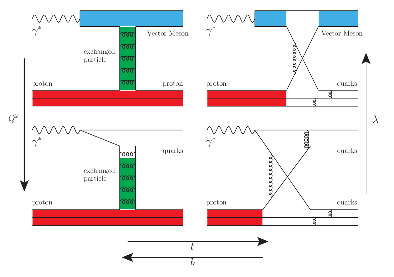
Since the probe of the interaction is the virtual photon, two things will happen. First, as increases the lifetime of its hadronic component decreases, therefore its coupling becomes more point-like. Second, the wavelength () of the virtual photon decreases. This concept is illustrated in Fig. 2.3 [22], in terms and .
When both and are small (top left panel of Fig. 2.3), the photon behaves as a beam of vector mesons which pass far away from the nucleon target (implying a large impact parameter ). The partons that may be exchanged have enough time to interact with each other and build various mesons.
At low and high (top right panel of Fig. 2.3), the small impact parameter corresponds to the hadronization length of the partons that are absorbed or recombined into the final state particles (within the interaction volume defined by ), before they hadronize. In simple terms, a pair of partons are exchanged between the meson and the nucleon and a gluon is exchanged between this pair of partons.
When increases, the resolving power of the photon increases and begins to probe processes which occur at shorter and shorter distances and can couple to the constituents of the exchanged particles. When is small (bottom left of Fig. 2.3), the photon probes only the quarks inside the pion that is exchanged between the proton and the outgoing meson. When and are both large (bottom right of Fig. 2.3), the quarks inside the proton are able to couple directly to the quarks inside the target because the wavelength becomes comparable to the impact parameter . The virtual photon sees the partons which are exchanged during the hard scattering.
This classical interpretation of the evolution of hard scattering was developed from Regge theory [20] (further discussed in Sec. 2.2.1), and has been successfully implemented to explain both meson photoproduction [20, 21, 22, 23] and electroproduction [22]. Excellent agreement has been achieved between model and data. A extension to this interpretation using instead of is expected in the near future [25].
2.2 Regge Trajectory Model
2.2.1 Regge Trajectory
This section gives a brief summary on the concept of Regge trajectories and some of their most important features.
The partial-wave method introduced in Refs. [33, 34] is a common methodology to analyze the scattering processes [35]. Consider the wavefunction in the form of
| (2.1) |
where is the angle between the wave vector and the position vector . In the case of bound states, the plane wave (first) term is absent. The form factor is written as a sum of partial waves as [19, 35, 36]
| (2.2) |
if
where is the orbital angular momentum quantum number and is the Legendre polynomial of degree . In the initial introduction of Regge theory [19], T. Regge generalized the solution for the solution of by treating as a complex variable. It was proven that for a wide class of potentials, the singularities of the scattering amplitude (simple poles ) in the complex plane were poles, now known as the Regge poles [17, 18, 37].
For real values of , , the partial-wave components of the scattering amplitude have only simple poles and are functions of ,
| (2.3) |
where is the Regge residue and is the position (Regge trajectory) of the poles. These poles correspond to the bound states or the resonances (baryons and mesons) [35].


The Chew-Frautschi plots [37] that project the spin quantum number () on axis and rest mass squared on the axis, for meson and baryon are shown in Figs. 2.4 (a) and (b), respectively. From the phenomenological point of view, the values of the resonances seem to be linearly correlated to the values over a set of particles of a fixed radial node number . Furthermore, Chew-Frautschi [33] were able to apply the Regge (pole) theory to investigate the properties of these linear trajectories () in the case of the strong interaction. This approach was a success, which allowed the Regge trajectory based models [17, 20, 23, 37] to predict the scattering amplitudes, the form factors and the experimental observables such as the cross sections which depend on the experimental kinematics variables such as , and .
In the Regge model, is also sometimes expressed as , or more commonly in terms of the Mandelstam variable as , or as . In the -channel (forward-angle) interaction, it is more convenient to use the representation, which reflects the forward-angle meson production. Similarly, is used for the -channel (backward-angle) interaction. Note that the condition or does not correspond to any physical particles (pole) because cannot be negative [38].


2.2.2 and Kinematic Limits
In pseudoscalar meson photoproduction ( GeV) reactions (such as ), the main feature involves a pair of strongly collimated peaks at forward ( 2 GeV2), and backward-angles ( 1 GeV2) [20, 21]. Similar to the particle exchange diagram for production shown in Figs. 2.5 (a) and (b), the -channel interaction (peak) is dominated by meson exchange and -channel interaction (peak) is dominated by baryon exchange. Note, this interpretation divides the interaction process into three separate regions with respect to (or ), and each of the three regions are dictated by different interaction mechanisms.
In the case of the electroproduction of the vector meson above the resonance production region ( 2 GeV) and large momentum transfer ( 2 GeV2), a similar feature in terms of the cross section behavior is expected as observed in pseudoscalar meson photoproduction. Currently, the strong forward-angle (-channel) peak has been experimentally measured [14]. However, the expected existence of the backward-angle (-channel) peak for vector meson electroproduction was not verified due to lack of experimental data until this Ph.D. work.
In this analysis work, the electroproduction of the vector mesons is divided in into three interaction regions with respect to (or ). The definition of the and limits are chosen based on similar definitions introduced by Ref. [20]:
- Low t Region:
-
1 GeV2,
- Low u Region:
-
1 GeV2,
- Large Emission Angle (LEA) Region:
-
1 GeV2 = 1 GeV or
0.5 GeV2 1 GeV.
Using the imposed momentum conservation constraints on the Mandelstam variables given by Eq. 1.7, if the experiment has fixed and values, the values can be converted into . Thus, a small value corresponds to a large value, and vice versa.

In terms of coverage, the upper limit of LEA region does not correspond to the maximum possible value: . The value is inside of the low region. The LEA upper limit is defined by the corresponding value of = 1 GeV2 (low upper boundary). Similarly, the upper limit of the LEA region in terms of coverage is defined by the corresponding value of = 1 GeV2 (low upper boundary). Depending on experimental kinematics, the boundaries between the three regions can vary, however, there is no overlap between the low and low regions.
Fig. 2.6 shows three regions in terms of the scattering angle in both Lab and CM reference frames. A -channel scattering process is used as an example. Note the boundary lines between different regions are for illustration purposes only, which do not correspond to any particular and values.
2.2.3 Regge Trajectory in Meson Production
In Regge-trajectory-based models, the standard treatment to take into account the exchange of high-spin, high-mass particles is to replace the pole-like Feynman propagator of a single particle (i.e. ) by the Regge (trajectory) propagator. Meanwhile, the exchange process involves a series of particles of the same quantum number (following the same Regge trajectory ), instead of single particle exchange. As an example, the Regge propagator for the pion trajectory is given as
| (2.4) |
where is the signature of the exchanged trajectory, and is the meson trajectory obtained from Chew-Frautschi plots such Fig. 2.4 (a). For vector meson (, and ) production, the Regge propagator can be constructed in a similar form.
The required exchanged particles (trajectories) for vector meson production are listed in Table. 2.1. For forward (-channel) production the dominant trajectories are (plotted in Fig. 2.4 a), and Pomeron () [20, 21, 22, 23, 24]; in the backward-angle scenario (-channel), the dominant baryon trajectory is [22, 23, 24].
For the forward hard scattering process where , the meson trajectories are assumed to approach (asymptotic limit) [20]. This is known as the saturation of the Regge trajectory. Note that the saturation effect also applies to the backward hard scattering process where . Saturation is an extremely important and profound assumption, which allows a smooth transition and extrapolation from the soft scattering amplitude at (or ) to the hard scattering amplitude () at (or ) [20]
| (2.5) |
or
| (2.6) |
where and are form factors of the two outgoing particles.
Examples of the Regge trajectory saturation of ( or ) for and are shown in Fig. 2.7. As the result of the saturation effect, the differential cross sections will tend to a plateau in the LEA range since the exponential -dependence () or -dependence () vanishes. In potential models, the saturation of the Regge trajectories (approaching when ) is closely related to the one-gluon exchange interaction between two quarks [20].

2.2.4 VGL and JML Models
With the introduction of the saturation of the Regge trajectory [20, 21], Regge-based models such as VGL [20, 21] and JML [22, 24] have become effective methods to deal with hard-scattering mechanisms in the non-resonance region ( and ) and have been successfully used to describe the meson photoproduction in and -channels, and the meson electroproduction in -channel.
The VGL model has been validated with experimental data of pion photoproduction from Refs. [39, 40, 41]. Fig. 2.8 shows the VGL model to data comparison. The peaks at -channel ( GeV2) and -channel ( GeV2 for GeV or GeV which corresponds to GeV2) were successfully described by the model. The experimental data features three distinctive regions across the range (as described in Sec. 2.2.2): the low region, the -channel peak dictated by the “soft” process of meson exchange; the LEA region, cross section plateau is the indication “hard” process; the region, -channel peak dictated by the “soft” process of hard baryon exchange. Here, the soft process refers to the photon probing the parton bound states (soft structure) inside of the nucleon; whereas the hard process describes the photon directly probing the point-like parton (hard structure). This classic interpretation offered by the VGL model on the soft-hard-soft transition carries special significance in understanding the evolution of the scattering process with respect to , and is elaborated in Sec. 2.1.1.

The , and meson photoproduction [42, 43, 44] and the electroproduction of data from CLAS [14] have demonstrated the predictive power of the JML model in the low and LEA regions. Compared to the VGL model, the JML model has included the dependence. The validation of the -dependence extension of the JML model came from electroproduction for GeV2 data from CLAS [14], and is further discussed in Sec. 6.10.2. The JML model was a successful milestone, significantly improving the knowledge regarding the hard scattering mechanism and establishing the direct linkage between kinematics variables (such as ) to the impact parameter [22, 23, 24] (described in Sec. 2.1.1).
Despite the great successes of Regge trajectory based models, there are some limitations that may require further research effort.
- •
As introduced in Sec. 2.1.1, the classical interpretation of is considered to be the resolving power of the probe and is inversely proportional to the virtual photon wavelength ( ). As increases beyond the effective range of the Regge model, the virtual photon wavelength (interaction radius) would decrease and start to directly couple to the parton structure. Currently, the upper limit of effective range of for the Regge theory has not been determined [14]. The study of the transition of the Regge theory in terms of would be beneficial to the understanding off the proton structure in terms of the quarks and gluons, and their interaction mechanism,
- •
In the case of the meson, the model predicts the dominance of the transverse component of the cross section at large value of [14],
- •
No calculation is available for -channel electroproduction. Furthermore, the behaviour of the differential cross sections inside the LEA region is also unknown. See further discussion in Sec. 7.2.
| Quark Composition | -channel | -channel | |
|---|---|---|---|
| f2, , | , - Interference | ||
| , f2, | |||
| Unknown coupling∗ |
2.3 GPD and TDA
As introduced in Sec. 2.1, Generalized parton distributions (GPDs) are an improved description of the complex internal structure of the nucleon, which provide access to the correlations between the transverse position and longitudinal momentum distribution of the partons in the nucleon. In addition, GPDs give access to the orbital momentum contribution of partons to the spin of the nucleon [26, 47].
In 1932, E. P. Wigner formulated a way to express quantum mechanical correlations using the language of classical statistical mechanics [48], which was later applied to describe the behaviour of quarks and gluons inside of the nucleon.
Assuming a one-dimensional quantum mechanical system with wave function , the Wigner function is defined as [49]
| (2.7) |
where is set to ; represents the position vector; is the momentum vector; represents the space-time separation. When integrating out the spatial information in , one can obtain the momentum density ; when integrating over the momentum space , one can obtain the spatial density . This is a unique functionality that allows the Wigner distribution (derived from the Wigner function) to contain the most complete (spatial and momentum) information about a quantum system, while respecting the Heisenberg uncertainty principle [26].
After constructing the “rest-frame” matrix element and averaging over all possible three-momentum transfer, the quantum phase-space quark distribution in a nucleon can be written as [49, 50]:
| (2.8) |
where is the Wigner operator, is the quark phase-space position; is the phase-space four momentum.
By integrating the transverse quark momentum information, the quark spatial structure of the proton is considered to be described by four independent leading twist helicity non-flip GPDs: , , , [49]. All of them are functions of longitudinal parton momentum , of the momentum transfer squared and of the skewness parameter , which is related to by . By integrating over the GPDs across the nucleon radius, one can access the electric and magnetic distributions of the nucleon. Note that there are four additional GPDs associated with the helicity flip, which are not discussed in this thesis. Correspondingly, the eight gluon GPDs can be obtained following the same principle [49].
Currently, there is no known direct experimental access to measure the GPDs [49]. The prime experimental channel to study the GPDs is through the Deep Virtual Compton Scattering (DVCS) and Deep Exclusive Meson Production (DEMP) processes [26]. Both processes rely on the collinear factorization scheme; an example of DEMP reaction: is shown in Fig. 2.9 (a). In order to access the forward-angle GPD collinear factorization (CF) regime ( interaction), the kinematics variables requirements are as follows: large , large , fixed and [49, 30].
Under the collinear factorization regime, a parton is emitted from the nucleon GPDs ( GPDs) and interacts with the incoming virtual photon, then returns to the GPDs after the interaction [49]. Studies [31, 32] have shown that perturbation calculation methods can be used to calculate the CF process (top oval in Fig. 2.9 (a)) and extract GPDs through factorization, while preserving the universal description of the hadronic structure in terms of QCD principles.


TDAs are the backward analog of GPDs, with their full name being the baryon-to-meson transition distribution amplitude ( TDA). TDAs describe the underlying physics mechanism of how the target proton transitions into a meson in the final state, shown in the grey oval in Fig. 2.9 (b). One fundamental difference between GPDs and TDAs is that the TDAs require three parton exchanges between TDA and CF.
As introduced previously, the GPDs depend on , and . The production process through GPDs in the forward-angle (-channel) and through TDAs in the backward-angle (-channel) are schematically shown in Figs. 2.9 (a) and (b), respectively. In terms of the formalism, TDAs are similar to the GPDs, except they require a switch from the impact parameter space ( dependent) through Fourier transform to the large momentum transfer space ( dependent), which brings a novel picture of the nucleon.
The backward-angle TDA collinear factorization has similar requirements: is fixed, the -momentum transfer is required to be small compared to and ; , which implies the and need to be sufficiently large. Based on these, the optimal range of study for the TDA model is 10 GeV2. The parameter is considered to encode new valuable complementary information on the hadronic 3-dimensional structure, whose detailed physical meaning still awaits clarification [30].
In both the GPD and TDA collinear factorization interaction diagrams shown in Fig. 2.9, apart from the GPD, TDA and collinear factorization, the parton structure (distribution amplitudes in terms of quarks) of the outgoing proton and meson have to be described. DA represents the meson distribution amplitude and DA is the proton distribution amplitude [30].
The and DA are based on the choice of the phenomenological solution for the leading twist nucleon DA and the corresponding value of the strong coupling represents a complicated problem. In the TDA calculation made for this Ph.D. thesis, the Chernyak-Ogloblin-Zhitnitsky (COZ) [51] and King-Sachrajda (KS) [52] DA models have been chosen. Both DA models have considerably different shapes from the DA asymptotic limit. Assuming the nucleon consists of three partons with momentum fractions, , and , the sum of the three distributions must equal to 1. If , then and the distribution of predicted by COZ, KS and asymptotic DA () are shown in Fig.2.10. Note that both COZ and KS DA models are capable of providing a description of the nucleon electromagnetic form factors.

The DA model is an important part to the TDA model prediction, and the predicted experimental observable can change significantly depending on the choice of the DA model. Therefore, the improvement of TDA formalism would rely on an accurate nucleon spatial distribution parameterized by the DA models. As more experimental data are collected to constrain the DA model during the 12 GeV era at JLab, significant developments in the GPD and TDA pictures are expected in the coming decades.
Due to its technical complexity, details regarding the nucleon distribution amplitude are excluded from this thesis, and further detail regarding the DA models can be found in Refs. [30, 51, 52].
2.3.1 Two Predictions from TDA Collinear Factorization
Through a private communication [54], a set of calculations matching the kinematics coverage of this Ph.D. work have been provided. Compared to the effective range of the TDA formalism (10 GeV2 [30]), the range of this Ph.D. work is much lower = 1.6, 2.45 GeV2. A quantitative comparison between data and model may nevertheless provide an intuitive demonstration of the predictive power of the TDA model (see Sec. 6.10.2).
The TDA collinear factorization has made two specific qualitative predictions regarding backward vector meson electroproduction, which can be verified experimentally:
- •
The dominance of the transverse polarization of the virtual photon results in the suppression of the cross section by a least (1/): ,
- •
The characteristic 1/Q8-scaling behavior of the transverse cross section for fixed , following the quark counting rules.
The L/T separated differential cross section is directly relevant to the validation of the TDA frame work. However, due to the limited the coverage, the second TDA prediction will be validated in the future studies.
Closing Remarks
Recall the question regarding the mechanism of producing the backward-angle that was raised in the beginning of this chapter. By using the interaction demonstrated in Fig. 2.3 (top left panel), an answer to the question can be reached. In order to generate backward-angle from the photon probe through the VMD effect, the interaction requires a low resolution (low ) and a high impact parameter (low or low ). Based on the kinematics of these data, in particular the values, one needs to explore mechanisms beyond the VMD.
In the intermediate energy and momentum transfer scenario, such as in this thesis, the virtual photon wavelength is much smaller than the proton radius. Thus, the backward meson is originated from the nucleon target through the exchange (or knock out) of a baryon. Therefore, the study of backward-angle (-channel) interactions at intermediate energy range contributes to the general understanding of dynamic properties of the nucleon.
Chapter 3 Experimental Apparatus
3.1 Overview
The Thomas Jefferson National Accelerator Facility11 1 12000 Jefferson Avenue, Newport News, Virginia. https://www.jlab.org/ (JLab) is a U.S. Department of Energy (DOE) user facility for fundamental nuclear physics research. Started in 1984 as a dedicated laboratory to study hadronic structure and the fundamental properties of nuclear matter, it has since become one of the world’s leading facilities for investigating the physics of quark-gluon interactions. JLab’s main research facility is the Continuous Electron Beam Accelerator Facility (CEBAF), which consists of a polarized electron source, an injector and two anti-parallel superconducting RF linear accelerators (linacs), connected to each other by two arc sections which contain steering magnets. The electrons are kept in a racetrack configuration during the acceleration process. A schematic diagram of the CEBAF is shown in Fig. 3.1.
Since 2011, JLab has undertaken a major upgrade to double its maximum beam energy to 12 GeV. By 2014, the first 12 GeV beam was delivered to Hall D which started the 12 GeV era of JLab operation. It is important to note that the experimental details discussed in this section are applicable to the 6 GeV era of JLab operation (prior to 2011).

3.2 Accelerator
From a semiconductor photocathode, polarized electrons are excited by circularly polarized laser light and accelerated by the Radio-Frequency (RF) resonant cavities of the accelerators. One particular feature of JLab is the continuous nature of the electron beam, with a bunch length of less than 2 ps. In addition, a fundamental RF frequency of 1497 MHz allows for three sequential electron bunches serving three independent experimental halls, each bunch having independent current amplitude during the 6 GeV operation period.
Conceptually, CEBAF is a linear accelerator that has been folded up in a design similar to that of a racetrack. Recirculation of the beam is possible up to five times to achieve the maximum beam energy: electrons are accelerated by the injector to an energy of 45 MeV and sent to the North Linac, where they gain an additional energy up to 600 MeV through acceleration on superconducting RF resonant cavities. From the North Linac, the electron beam is bent through the east arc and guided through the South Linac, where it gains up to another 600 MeV.
After the electron beam exits the South Linac for a given pass, the Beam Switch Yard (BSY) alternately delivers one out of every three bunches of electrons to each of the three experimental halls, or recirculates them through the west arc for an additional pass through the linacs.
During the JLab 6 GeV era operation, the maximum energy gain of the CEBAF was 1.2 GeV per pass, corresponding to a nominal energy of 6 GeV. Each linac consisted of 20 cryomodules, each of which contained eight superconducting niobium cavities cooled by liquid helium at 2 K. The same linacs were used for the acceleration in each circulation. Nonetheless, the beams from different passes were split into different vacuum pipes before being steered by the steering magnets and traversing through the recirculating arcs. Before the entering the linac, the beams from different passes were recombined. This unique configuration allowed the experimental halls to run simultaneously at different energies.
The CEBAF accelerator produces beams in bunch lengths of less than 2 ps, which occur at a frequency of 1497 MHz as a result of the RF power used in the resonating cavities. During the 6 GeV operation period, every third pulse was delivered to each of the experimental halls resulting in one pulse every 2 ns, which corresponded to a beam frequency of 499 MHz. The RF separators at the BSY separated the beam pulses after each linac pass. It should be noted that at this rate, the beam delivery can be effectively considered continuous. The continuous beam property is critical for a coincidence experiment such as Fπ-2, which requires a high precision and high luminosity to insure reliable extraction of the cross section with acceptable statistical uncertainty.
To achieve the same luminosity, a non-continuous (pulsed) linac such as SLAC22 2 Stanford Linear Accelerator Center (SLAC) National Accelerator Laboratory, 2575 Sand Hill Rd. Menlo Park, CA 94025. https://www6.slac.stanford.edu/ would require a higher electron density within a bunch and longer bunch width within the operation window. This would significantly increase the random coincidental backgrounds and reduce the timing separation. Conceptually, the real coincident events would be diluted by the random coincident events and raise the statistical uncertainty for the cross section. Thus, performing a coincidence measurement is not feasible for with a non-continuous linac.
3.3 Hall C
Fig. 3.2 shows an overhead schematic layout of experimental Hall C during the JLab 6 GeV operation. The hall has a nearly circular geometry with a diameter of 32 m. A large fraction of the experimental hall is located underground and it is well shielded to contain the hazardous level of radiation.
The standard Hall C apparatus consists of two magnetic focusing spectrometers: the High Momentum Spectrometer (HMS) shown in Fig. 3.5, and the Short Orbit Spectrometer (SOS) shown in Fig. 3.5. Fig. 3.3 shows an image of Hall C during the Fπ-2 experiment, where the critical spectrometer and beamline components are labelled.
The HMS optics configuration consists of three superconducting quadrupoles followed by a dipole and has a path length of approximately 26 m from the target to the focal plane. In contrast, the SOS optics consists of three resistive magnets and has a path length of 10 m, which is adequate for the detection of short-lived particles at low momentum. The momentum resolutions of the HMS and SOS are better than 10-3 m and the horizontal angular resolutions are better than 2 mrad. The designed maximum central momenta for the HMS and SOS are 7 and 1.74 GeV/c, respectively. The standard instrumentation in Hall C has been used successfully for a variety of experiments requiring the full CEBAF beam current of 200 A.


3.4 Beamline
For a precision L/T-separation experiment such as Fπ-2, the characteristic (profile) of the electron beam is an important factor that needs to be monitored throughout the experiment. In this section, the techniques and apparatus for determining the beam position, current and energy information are briefly introduced.

3.4.1 Beam Position Monitors
The monitoring of the position of the beam in the Hall C arc and beamline is accomplished with Beam Position Monitors (BPM, as shown in Fig. 3.6. The BPM monitors consist of resonating cavities with a fundamental frequency to match both the MHz accelerator beam pulse frequency and the MHz pulse frequency into Hall C. Each cavity has four antennas which are rotated by with respect to the horizontal and vertical axes to minimize damage caused by the synchrotron radiation. The angle was chosen is due to the beam being focused in horizontal and vertical directions by quadrupoles along the beamline. The amplitude of the signal picked up from the fundamental frequency by each antenna allows for the determination of the relative position of the beam [57].
The primary beam steering is guided by the BPMs located in Hall C, and additionally, the BPMs closest to the target (H00A, H00B, H00C) were also monitored to ensure precision. The beam position was set based on information from spectrometer optics data and it varied for each of the four beam energies used during the Fπ-2 experiment. Note that the BPM coordinates do not represent the absolute position of the beam and are chosen based on the requirement of simultaneous mid-plane symmetry in both spectrometers.
The beam position at the target location can be determined by combining the projection of any pair of BPMs. During the experiment, BPM C was determined to be unreliable, so that for all subsequent calculations only BPM A and BPM B were used. Note that the typical size of the position variation at the target was less than 0.5 mm.
The beam position and direction at the entrance, middle and the exit of the Hall C arc are measured using the high resolution wire sensors (harps) system. The harps system consists of two vertically and one horizontally oriented wires in a non-stationary frame. During a ‘harps scan’, the vertical wires move across a low current beam at the same time, then followed by the same action from the horizontal wires. The signals generated at each wire as they are intercepted by the beam are recorded by an Analog to Digital Converter (ADC) unit. The corresponding position of the wire intercepted is then determined by a position encoder.
The superharps system is an upgrade of the harps system, including absolute position readout electronics, a dual beam profile detection system with two analog pick-up channels and a vibration-free support system. The harps system and its operation are described in more detail in Ref. [58].
3.4.2 Beam Energy Measurement

The energy of the electron beam in Hall C is measured using the deflection of the beam in a known magnetic field in the Hall C arc. The technique makes use of the fact that an electron traversing a constant magnetic field moves in a circular trajectory, where its radius depends on the strength of the magnetic field and the electron momentum. The arc method uses the arc magnets as a type of spectrometer and the beam position measurement to determine the deflection of the beam in the section of the beamline between the BSY and the hall entrance. The conceptual drawing of such instrumentation is shown in Fig. 3.7. The blue dashed box in Fig. 3.6 (top right corner), shows the Hall C arc (3C Arc).
This measurement cannot be performed simultaneously with regular data taking because it requires all the focussed elements to be turned off and degaussed (neutralizing the residual magnetic field). The beam position and direction at the entrance, middle and the exit of the arc are measured using the superharps system. The bend angle of the Hall C arc () was measured to be . The beam is then steered so that the central trajectory and the beam energy can be determined from the electron momentum using:
| (3.1) |
where is the electron charge and is the magnetic field in the dispersive elements. The extraction of the beam energy from the field integral requires the knowledge of the magnetic fields in the arc dipoles. For this reason, one of the dipoles in the Hall C arc has been field-mapped as a function of current.
The remaining eight dipoles are calibrated relative to the reference dipole assuming similar field maps. Using the value of the field integral, the beam energy can be determined with a precision of [55]. A more detailed description of the energy measurement of the beam using the arc method is documented in Ref. [59].
3.4.3 Beam Current Monitors
The Fπ-2 experiment uses two Beam Current Monitors (BCM) that measure the electron beam current delivered to Hall C. The primary BCMs (BCM1 and BCM2) are cylindrically shaped waveguides tuned to the frequency of the beam. The geometry of these cavities was designed to be excited by the 33 3 Transverse electromagnetic (TEM) is a mode of propagation where the electric and magnetic field lines are all restricted to directions normal (transverse) to the direction of propagation. The subscript refers to the resonating mode of the standing (EM) wave created inside of the superconducting cavity. mode of the electron beam pulse frequency [55]. This mode has the particular advantage that its magnitude changes slowly with respect to the position of the beam within the cavities. The output voltage levels of the waveguides are proportional to the beam current when the waveguides are tuned to the frequency of the beam.
The resonant frequency of the cavities is sensitive to the temperature fluctuations, since the current monitor cavities can thermally expand or contract due to temperature changes. To minimize these effects, the temperature is stabilized by thermally insulating the beam monitor cavities at a constant value of C. The cavity temperature was checked during each shift and found to be oscillating within the range of C. Note that the temperature of the readout electronics can also affect the current measurement. In order to minimize this effect, the electronics room was maintained at a nearly constant temperature throughout the experiment.
Both BCM1 and BCM2 exhibit reasonable gain stability as a function of time. Nonetheless, to minimize drifts in the gain, both BCMs are calibrated to an absolute standard device at regular intervals. The calibration is performed using an Unser current monitor [60], which is a parametric DC current transformer. The Unser monitor has an extremely stable gain, but suffers from large drifts in the offset on short time scales. Thus, the Unser monitor cannot be used alone to measure the beam current reliably on a run-to-run basis. The resonant cavity BCMs were calibrated by taking dedicated runs with periods of no beam (the purpose was to monitor the Unser zero/baseline) interspersed with periods of beam at various currents.
During the Fπ-2 experiment, the currents ranged from 10 to 110 A, and the actual current values were continuously adjusted. The BCMs are generally stable enough so that calibrations have to be performed only infrequently during the experiment. The run-to-run uncertainty in the current, as measured by BCM1 and BCM2, is estimated from a combined analysis. The averaged current drift between calibrations was found to be on the order of at 100 A [55]. Considering in addition the normalization uncertainty from the Unser monitor, which is estimated to be , results in an absolute uncertainty for the charge measurement of .
3.4.4 Modification to Beamline
The beamline of Hall C was modified for the Fπ-2 experiment by adding a small diameter beam pipe installation downstream of the target, to allow for data taking at the smallest possible angle between the beam line and the spectrometers in particular the HMS. With this particular geometry (at small SOS central angles), the beam pipe is susceptible to magnetic fields from an unshielded edge of the SOS dipole magnet. The presence of these magnetic fields was confirmed prior to the experiment from measurements at a momentum setting of 1.74 GeV/c [53, 61]. The dominant fields are parallel to the dipole yoke and oriented along and perpendicular to the spectrometer axis. The contribution from magnetic fields vertical to the magnet yoke and perpendicular to the spectrometer axis are smaller [62].
Since a beam deflection that exceeds the upstream beamline aperture can cause damage to one of the flanges of the Hall C beam dump due to an excessive deposition of energy, there was a concern about the beam deflection at the diffuser at the exit of the hall. The deflection of the beam was calculated for different kinematic settings using a magnetic field map data. In the calculations, a SOS momentum of 1.74 GeV/c and a beam energy of 5 GeV were assumed. The deflection at the smallest angle for Fπ-2 experiment was determined to be 4 mrad from the target centre [63, 64]. The vertical deflection of the beam at the diffuser was addressed with magnetic shielding of the downstream beam pipe. Two layers of magnetic shielding foil were also installed around the beam pipe in order to reduce the value of the field integral and its corresponding beam deflection.
3.5 Targets


The Hall C target system contains a three-loop cryogenic target (cryotarget) stack mounted together with optics and “dummy” targets on a target ladder enclosed in a high vacuum scattering chamber. Fig. 3.8(a) shows a schematic drawing of the target stack configuration inside of the scattering chamber. The solid target ladder consists of five carbon and two aluminum foils at different positions (=0 cm, =2 cm, =7 cm) along the beam direction [55, 65], here is along the beam direction from the BSY to the beam dump, and the center of the target station is at = 0 cm. The two aluminum foils situated at = 2 cm constitute the “dummy target”, which is used to quantify the experimental yield from the aluminum cryotarget cell wall. Note that the dummy target is 7.022 times thicker than the nominal thickness of the cryotarget cell walls. The remaining solid carbon foils are used with beam incident on two or five (“quintar”) foils simultaneously for the purpose of calibrating the spectrometer optics properties.
The average energy deposition in the cryotarget is relatively large (4 MeV cm2g-1), while the diameter of the incident electron beam is relatively small ( mm). The electron beam needs to be rastered44 4 Beam rastering technique is a standard procedure to uniformly distribute the electron beam onto the cryogenic target, thus, minimizing the localized heat deposit. This is generally achieved by using a combination small dipole magnets upstream of the cryogenic target. to a mm2 profile in order to distribute the energy in a more uniform manner across the cryotarget volume, since the local heating can lead to a target density fluctuation (i.e. a target boiling effect). The rastering profile used during the Fπ-2 experiment consisted of a constant and uniform pattern in contrast to the sinusoidal pattern used in previous experiments [55]. This system is described more fully in Refs. [66, 67].
3.5.1 Cryogenic Targets: LH2
The cryogenic targets were each held inside of a cylindrical “tuna-can” cell, of 4 cm in diameter, oriented vertically as shown in Fig. 3.8(b). Each target cell occupies one of the three available loops. During the Fπ-2 experiment, the loop 1 was empty, while loops 2 and 3 contained liquid hydrogen (LH2) and liquid deuterium (LD2), respectively. Both cryotargets used the same coolant supply (liquefied helium) and were cooled on the cryotarget ladder simultaneously. The End Station Refrigerator (ESR) supplied the helium at 15 K and the coolant flow to the individual loop was controlled by the target operator using Joule Thompson (JT) valves.
The cryogenic coolant is circulated continuously through the heat exchanger from the target cell. Low and high power heaters are controlled by a Proportion, Integral and Derivative feedback system, keeping the LH2 at 19 K. During low current or beam-off periods, the target control system regulates the cryotarget temperature by replicating the power deposition of the electron beam using high power heaters, while the target fluid moves continuously through the heat exchanger around the target cell. From Fig. 3.8(b), each target cell is 3.95-4.02 cm long in the beam direction, with cell walls made from aluminum alloy T6061 and of a thickness of 0.013-0.014 cm. The alloy used in manufacturing the aluminum dummy targets is AI-T7075, a higher strength alloy. More information regarding the cryotargets’ mechanical structure, composition and design can be found in Refs. [68, 69, 70].
During the experiment, conditions such as the flow rate and temperature of the cryogenic fluid, thermal expansion (contraction) and boiling effects can affect the target density and volume. In order to minimize these effects, the cryotarget (such as the LH2 target) at a density of 0.07230.0005 mg/cm3 is kept at a nominal operating temperature of 19 K, which is around 2 K below the boiling point. Measuring the target length at room temperature and doing the offset corrections for the target from the center of the beamline and thermal contraction (), the real length of the cell in the cooled-down state is calculated to be 3.980.01 cm [55, 65].
As the electron beam traverses the target, significant energy per unit area is deposited. The energy deposition from the electron beam in the target is predominately due to the ionization process and can be estimated by the Bethe-Bloch formula [1]. Assuming a 100 A current electron beam accelerated to 6 GeV of energy, the estimated stopping power in the LH2 target is around 4 MeV cm2/g [71]. The LH2 target density and length are 70.8 mg/cm3 and 3.98 cm, which yield energy loss of 1.1 MeV. The power loss is equivalent to a 100 Watt light bulb (assuming most of the energy is converted into heat). In order to keep the LH2 target below the 20.28 K boiling temperature, and avoid localized density fluctuation, a large amount of cooling power ( 100 Watts) is required. In addition, the electron beam is rastered in a uniform pattern to distribute the heat evenly across the tuna can target (if electron beam radius is less than 0.5 mm, the power per unit area can reach Watts/m2).
A 100 A current 6 GeV electron beam on a carbon target does not require target density (temperature) correction or beam rastering. Since the carbon material has a lower stopping power of 2 MeV/g/cm2 [71], the energy loss in the material is estimated to be 0.34 MeV, which corresponds to a power output of 34 Watt. Note that the carbon target thickness is taken as 0.173 g/cm2 [65], in combination with the high melting temperature of the carbon material (3550∘C) [72]. The carbon target data are perfect to study the rate dependent efficiencies such as tracking efficiency under high trigger rate environment ( 500 kHz).
3.5.2 Target Thickness
The cryotarget thickness and associated uncertainties are listed in Table 3.1, where the cryotarget length at room temperature is corrected for thermal contraction of the aluminum cell walls and the offset of the cryotarget from the surveyed position (3.42 mm). The actual target thicknesses for these targets were also corrected for the beam offset from the target center at each kinematic setting, the target thickness uncertainty is the quadrature sum of uncertainty on the target length and on the target density. The total target thickness is determined using the target cell geometry at operating temperatures in combination with the target density derived from cell temperature and pressure.
For the cryotarget, the cell temperature was kept constant to 100 mK within the operation temperature (19 K) during the Fπ-2 experiment. The dominant uncertainty in target density is due to the thermal expansion and contraction, and it is about . Note that the uncertainty contributions from the measured temperature are negligible. The uncertainty for the outer diameter of the target cell at room temperature was measured to be . The uncertainty for thickness of the cell walls was determined to be mm [55].
| Target | Target length (cm) | Target thickness (g/cm2) |
|---|---|---|
| LH2 |
The target length is sensitive to the size and the form of the raster pattern and the central position of the beam from the target center. The reduction of effective target length due to the constant raster pattern was determined to be [55]. Initial target survey results and measurements of thermal effects, like vacuum motion and target cool-down motion, indicate that the target cells were on average located at 3.420.50 mm (with the beam right facing downstream) relative to the nominal beamline. Optics data and information from the beam position monitors suggest that the beam was offset between 0.15 and 2.00 mm in the same direction for the four different kinematic settings. In the worst case deviation of the beam from the target center, the correction of the effective target length is . The variation in target thickness due to the central beam position between high and low settings is . Additional uncertainties to the target thickness are given by the purity of the target gas and dynamic effects such as target heating due to energy deposited by the electron beam. To determine the target purity, samples of the target materials were examined after the experiment. Both cryotarget purities were found to be , so no correction was assigned [55].
Localized target density fluctuations due to heating effects can have a significant effect on the average density of cryotargets. The rastering of the beam reduces local density fluctuations of the liquid targets, but cannot eliminate them entirely. The change in luminosity due to beam heating was measured by comparing yields at fixed kinematics as a function of beam current. To account for the net reduction in measured target density due to localized target boiling, a correction factor is applied. Taking into account the uncertainty in the beam current, the total uncertainty in the target density is on the order of . Based on the target boiling study in Sec. 5.3.5, no significant target density reduction due to localized heating was found. Thus, no target boiling correction factor was applied.
In order to understand and subtract the thin aluminum wall (target chamber) contribution to the experimental yield, data runs with a dummy target were used to correct experimental data. The dummy target thickness was designed to be greater than the thickness of the wall of the target cell, thus reducing the dummy target data taking period.
According to the information documented in the Fπ-2 target configuration technical report [65], the normalized dummy target experimental yield has to be corrected by the following factor:
| (3.2) |
Note that the percentage uncertainty for the dummy-target ratio is the quadratic sum of the percentage uncertainties in LH2 target cell wall thickness and dummy target thickness, and is calculated to be 1%.
3.6 Detectors
The detector package layout in the HMS and SOS are very similar. As an example, the conceptual drawing of the HMS layout is shown in Fig. 3.9. The detector package consists of two horizontal drift chambers for the track reconstruction, four scintillating hodoscopes used for generating the triggers and measuring the time-of-flight (TOF), the threshold gas Cherenkov detectors and lead-glass calorimeters used for particle identification. The HMS detector package also includes an aerogel Cherenkov detector used for separating protons from pions. - separation is performed using the gas Chereknov detectors in both spectrometers. A complete review of the detector packages, including detailed geometry and performance, can be found in Ref. [73].
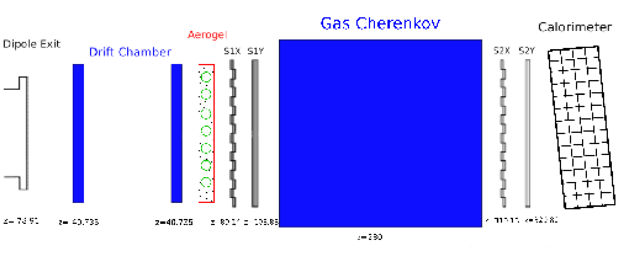
3.6.1 Drift Chamber
The drift chambers are used to measure the horizontal and vertical angles and positions of the charged particles before and after the focal plane, in order to determine their momenta and trajectories. The basic operation principle is as follows: charged particles induce ionization of the atoms inside the gas chambers and the free electrons are produced due to the ionization process. These free electrons are eventually captured by the sense wires. A good spatial resolution is achieved by measuring the deviation in the electron drift time. The electric field inside of the gas chamber is required to be a very specific configuration, which is achieved by surrounding the sense wires with non-sensed wires at high voltage. The trajectory information of the two sets of chambers are combined to determine the trajectory of the charged particles through the focal plane.
The HMS spectrometer is equipped with a pair of drift chambers and each consists of six wire planes. For each chamber, the wire planes are ordered , , , , , . The and planes determine the dispersive (vertical) coordinates of the particle trajectory, while two and planes determine the non-dispersive (horizontal) track position. The and plane wires are at with respect to the plane, the purpose of these wires is to enhance the tracking resolution in the vertical direction. The cell spacing is 1 cm and the position resolution is approximately 150 m per plane. Note that the HMS has better resolution in the dispersive direction due to its wire plane configuration. The two drift chambers are placed at a distance of 40 cm before and after the focal plane. The ionizing medium in the HMS drift chambers is an argon-ethane mixture of 1:1 ratio, which is controlled by a gas handling system located on the outside of the experimental hall.
The design of the SOS drift chamber is similar in design to the HMS drift chambers. The SOS is also equipped with a pair of drift chambers consisting of six planes of wires. The wire planes are ordered , , , , , . In the same fashion as the HMS, the and planes determine the vertical particle trajectory. The and planes are rotated 60∘ clockwise with respect to the coordinate determined by the and , while the and planes are rotated 60∘ counterclockwise. Similarly, in the HMS the matched planes are offset by 0.5 cm perpendicular to the sense wire direction to resolve the left-right ambiguity in the case of multiple hits in both planes. An argon-ethane mixture of 1:1 ratio is also used for this chamber.
3.6.2 Hodoscopes
Both HMS and SOS are equipped with four planes of scintillator hodoscopes divided into pairs of - planes. Each pair contains one plane segmented in the vertical and one plane segmented in the non-dispersive direction (horizontal plane). Each plane is composed of several components: the detector paddles made of long narrow strips of scintillator material with PMTs attached to both ends. The scintillator paddles are arranged in an overlapping configuration to eliminate gaps between the elements.
The principle of scintillation detectors can be summarized as follows: charged particles travelling through the scintillator material ionize atoms in the medium. The emitted electrons interact with the scintillating material, exciting molecules to higher energy levels. The excited molecules return back to the ground state (de-excitation) by emitting photon energy. The emitted photons propagate through the material via total internal reflection and are detected by PMTs attached to either ends of the paddle.
The reflecting material is aluminum foil for the HMS and aluminized mylar for the SOS scintillator elements. The HMS scintillator paddles have dimension of cm2 (width thickness) and the dimensions in the SOS are cm2 for the planes and cm2 for the planes. The length of the paddles depends on the spectrometer and their location and orientation in the detector hut. It should be noted that the scintillator paddles are shorter in the SOS, thus, resulting in a generally better time resolution per plane than in the HMS, due to reduced attenuation. However, the overall TOF resolution remains similar because of smaller separation distance between the front and back pair of planes in the SOS.
The arrangement of the two pairs of planes is similar in both spectrometers. However, the separation between the front and the back planes and the order of the four planes is different. In the HMS, the first plane is segmented vertically ( planes) and the second plane segmented horizontally ( planes), with separation of 220 cm between the front and back pair. The plane order is reversed in the SOS and the pair separation is 180 cm.
The main purpose of the scintillator hodoscopes is to provide the raw trigger for the data acquisition system and to determine the particle velocity by measuring the TOF between the front and back planes. The hodoscope signals are read out through a combination of Analog to Digital Converters (ADCs), discriminators and Time to Digital Converters (TDCs), and signal logic modules. Note that the electronics use leading-edge discriminators, which will result in timing shifts due to the difference in energy deposited (signal pulse height), also known as the time-walk effect. The timing information from each scintillator paddle is corrected for the time-walk effect and (timing) offset using a software calibration routine. The detailed description of this routine can be found in Ref. [73].
3.6.3 Cherenkov Detectors
As an important part of the standard particle identification (PID) package, both spectrometers are equipped with gas threshold Cherenkov detectors. The primary objective for both detectors is to perform - separation.
The basic working principle of the threshold Cherenkov detector relies on the Cherenkov effect, which is described by classical electrodynamics [6]. Cherenkov radiation is emitted when a charged particle traverses a dielectric medium of index of refraction with velocity ratio that is faster than the light speed inside of the medium (). The Cherenkov radiation angle can be calculated as
The emitted Cherenkov light is reflected from parabolic mirrors inside of the detector and focused onto the sensitive area of the photon multiplier tubes (PMT).
The () threshold property of the Cherenkov radiation allows the possibility to adjust the dielectric (gas) medium in the detector to allow identification of electrons and pions over a wide range of momentum settings. Although the separation of electrons and pions is highly efficient, the rejection of pion events is complicated by the presence of knock-on (secondary) electron due to multiple scattering inside of the detector. The secondary electrons (-rays) are produced when a proton or pion interacts with the material in front (or inside) of the Cherenkov gas and subsequently results in a hit in the Cherenkov detector. The mis-identification of proton due to -ray is a significant effect during the analysis, and further detail can be found in Sec. 5.3.9.
The HMS Cherenkov detector is a cylindrical tank holding two mirrors and two PMTs. The detector design allows for gas pressure in the tank above and below atmospheric pressure. Therefore, the detector can be used for - separation at atmospheric pressure or below, but it can also be used to separate pions from protons using Freon-12 (CCl2F2) above the atmospheric pressure. During the Fπ-2 experiment, the HMS Cherenkov was filled with C4F10 gas at a pressure of 0.47 atm. The corresponding index of refraction at this pressure is 1.00066, which yields an electron Cherenkov radiation (momentum) threshold of 14 MeV/c and a pion threshold of 3.8 GeV/c.
The SOS Cherenkov detector design is similar to the that of the HMS, but contains four mirrors and four PMTs. The Cherenkov medium was Freon-12 at a pressure of 1 atm. The corresponding refractive index at this pressure is 1.00108, which results an electron Cherenkov radiation momentum threshold of 11 MeV/c and a pion threshold of 3 GeV/c. Note that such momentum thresholds exceed the SOS maximum central momentum by about a factor of two.
3.6.4 Lead Glass Calorimeter
The primary objective of the lead glass calorimeter is to provide an additional means of selecting and separating electrons from pions. The lead glass calorimeter is positioned at the back of the detector hut for both spectrometers. The calorimeters use cm3 blocks arranged in four planes, and stand 13 and 11 blocks in both height and width in HMS and SOS, respectively. The entire detector is tilted by 5∘ relative to the central ray of the spectrometer to minimize losses due to particles passing thought the gaps between the blocks. To ensure light tightness, each block is wrapped in aluminized mylar and tedlar film. The calorimeter signal from each block is read out by PMTs attached at one side.
Particle detection using electromagnetic calorimeters is based on the production of electromagnetic showers in the lead glass material. As particles enter the calorimeter, they interact with nuclei inside the lead glass material and radiate photons via the bremsstrahlung process. The bremsstrahlung photons produce electron-positron pairs that also radiate photons (by either secondary bremsstrahlung or Cherenkov processes). The particular choice of the calorimeter thickness ensures that incident electrons or positrons deposit all their energy in the particle shower. The light radiated by the charged particle is collected by PMTs through internal reflection, and the amplitude of the signal is proportional to the incident momentum of the primary charged particles. Pions and muons entering the calorimeter do not produce bremsstrahlung showers, and instead they deposit a constant amount of EM shower (300 MeV) in the calorimeter. Similar to pions, protons will not generate bremsstrahlung showers, and deposit even less EM shower. However, pion, muons and protons can undergo nuclear interactions in the lead glass and produce particle showers similar to the electron-positron induced particle showers.
The separation of electrons from other particles, such as decayed pion events, is based on the normalized energy deposited in all layers in the calorimeter. During the Fπ-2 experiment, the SOS calorimeter was used in combination with the SOS gas Cherenkov detector to select electrons and exclude events.
The first layer of the calorimeter stack carries a unique significance, since it contributes two important trigger conditions: PRHI and PRLO, which are defined and explained in Sec. 3.7.
3.6.5 HMS Aerogel Cherenkov Detector
In addition to the standard PID detectors, the HMS has an aerogel threshold Cherenkov detector that provides adequate hadron identification for the spectrometer central momenta above 3 GeV/c. The primary objective of the HMS aerogel Cherenkov detector (ACD) is to separate pions from protons at high momentum (3 GeV/c). Different from the low momentum region, the - separation at high momenta is not effective by using the standard TOF method (examine the velocity of the particle) due to the decreased timing separation: , where is the central momentum setting of the HMS. Similar to the gas Cherenkov detector, the principle of the ACD is based on the threshold Cherenkov radiation, which depends on the refractive index of the dielectric medium.
The dielectric medium in the HMS ACD was specifically chosen to perform - separation from 3.0 - 4.6 GeV/c. Aerogel is a hydrated silicon oxide of molecular structure: n(SiO2)+2n(H2), and its density ranges between 0.04 - 0.20 g/cm3. The hydrate surrounding the aerogel molecule yields an average refractive index between gases and liquids. During the Fπ-2 experiment, aerogel with refractive index of was used ( was also available), which yields a Cherenkov radiation threshold of 0.565 GeV/c and a proton threshold of 3.802 GeV/c. The threshold momenta for muons and kaons are 0.428 and 2.000 GeV/c, respectively. The highest HMS momentum setting during the Fπ-2 experiment was 3.336 GeV/c, so that - separation can be done adequately.
The HMS ACD consists of 650 tiles ( cm3) arranged into nine 5 mm honeycomb sheets stacked in a cm2 tray. The individual layers were offset with respect to each other by 2-3 cm to minimize the loss of particles passing through the detector without hitting any aerogel material. The Cherenkov radiation generated by charged particles passing through the aerogel is collected by 165 inch Photonis XP4572B PMTs55 5 https://www.photonis.com/ mounted on each side of the reflecting diffusion box.
The reflective surface results in multiple internal reflections of the produced Cherenkov photons before detection. The aerogel tiles were made light-tight by wrapping them in reflective material, except for the surface facing the diffusion box with Millipore paper. To ensure high reflectivity from the internal walls, the inside of the diffusion box was covered with Membrane GSWP-0010 Millipore paper66 6 http://www.emdmillipore.com. The entire assembly of tiles was held in place by a 100 m stainless steel wire. Further details on the design and testing of the HMS ACD can be found in Ref. [74].
3.7 Trigger System

The purpose of this section is to provide a basic introduction to the trigger system used during the Fπ-2 experiment, and also introduce some terminology such as pre-scale factor (PS) and pre-trigger.
A schematic diagram for the single-arm trigger logic for the HMS (the SOS is similar) is shown in Fig. 3.10. The purpose of the single arm trigger logic is to generate a pre-trigger signal when a particle arrives. The pre-trigger signals from both spectrometers are fed into a trigger supervisor circuit (TS). The single arm (HMS or SOS) and two arm coincidence trigger signals are formed depending on the state of the TS (GO, ENABLE or BUSY). Both triggers and pre-triggers are fed into scaler modules, providing information such as the electronic dead time (EDT) and computer dead time (CDT). The TS takes in all the pre-trigger and trigger signals and effectively controls the readout of all detector ADCs and TDCs for the events. In order to reduce EDT and CDT, especially at high event rates, a pre-scaling circuit is introduced to control how frequently an event type is selected to proceed to the TS. One can adjust the event selection frequency by changing the pre-scale factor, i.e. a PS factor set to 1000 means a given event type is forwarded to the TS once every 1000 events.
3.7.1 HMS Pre-trigger
Fig. 3.10 shows the schematic diagram of the HMS pre-trigger that is composed of signals from different HMS detectors. The main component of the HMS trigger are the signals (or information) from the hodoscopes (scintillators) that are indicated as SCIN or STOF.
The SCIN (“3/4”) signal requires a signal from three out of four layers from the hodoscope scintillator planes within a timing window of 50 ns. The advantage of using this trigger configuration is to minimize the impact of the single layer of hodoscope efficiency on the trigger efficiency. The practical experiences gathered from the previous experiments [13, 75] have demonstrated the effectiveness (a consistent reliable high efficiency) of this trigger configuration. In addition, 3/4 signals is a good methodology to monitor the performance of the hodoscopes during the experiment.
The signal condition STOF is satisfied when two of the scintillator planes independently give a signal, with one signal from the front and other signal from the back hodoscope plane. This is the minimum condition for the computation of the TOF information of a detected particle. Note that satisfaction of the signal condition SCIN would imply the automatic satisfaction of STOF.
If the scintillator signal is present, the pre-trigger signal can be formed in one of the two different configurations: ELLO and ELHI. The ELHI configuration is formed if all three of the following signals are present: the SCIN signal, the PRHI signal and SHLO signal. Both PRHI and SHLO signals are formed at the calorimeter, where the former is satisfied when the signal from the first layer of the calorimeter exceeds a particular “high” threshold and the latter is formed when the total energy deposited in the calorimeter is above a particular “low” threshold. The ELLO pre-trigger requires a two out of three coincidence of SCIN, PRLO and STOF, where PRLO is defined as a signal from the calorimeter and the energy deposited in the first layer of the calorimeter exceeds a particular “low” threshold. In addition, absent of the Cherenkov signal: CER is used as the signal veto for the ELLO, meaning if CER is not present the ELLO signal will be vetoed. Further clarification regarding the PRHI and PRLO thresholds, can be found in Ref. [55].
As shown in Fig. 3.10, there are four different pre-trigger options: 1. Standard ELREAL, 2. prescaled 3/4 pion trigger PIPRE, 3. “Open” 3/4 trigger SINC and 4. Pion trigger, 3/4 with Cherenkov veto PIONHI.
The logic-OR of ELHI and ELLO forms the electron pre-trigger or ELREAL signal. The advantage of using a two path electron pre-trigger is to reduce sensitivity due to particular hardware in either the Cherenkov detectors or the calorimeter. Two copies of ELREAL are formed, of which one signal is sent to the HMS PRETRIG module where it is logic-ORed with the pre-scaled pion signal, PIPRE. The PIPRE signal is effectively a pre-scaled 3/4 SCIN and is formed to ensure that a sample of pions is recorded by the data acquisition system to allow determination of PID efficiencies for Cherenkov and calorimeters. The PRETRIG signal is split into four copies after the PRETRIG module, called PRE50, PRE100, PRE150 and PRE200. These four copies of PRETRIG are used for determination of the electronic live time (ELT). Detailed explanation of these four different pre-trigger modules and ELT analysis can be found in Sec. 5.3.2.1.
The fourth pre-trigger option PIONHI was implemented during the Fπ-2 experiment. PIONHI is satisfied by the presence of the 3/4 SCIN signal in absence of CERHI, which is the HMS Cherenkov signal with a high threshold for the detected number of photo-electrons N in order to reject a larger fraction of electrons. The PIONHI is sent to the HMS PRETRIG module and is read out in the scalers and TDCs. During the first part of the experiment, the pion trigger condition was implemented as PIONHI logic-ORed with the SCIN signal to allow for cautious monitoring of the Cherenkov veto signal. Later in the experiment, the pion condition was reduced to PIONHI. The Fπ-2- analysis by T. Horn [55] shown no significant difference in terms of data quality between these triggers.
3.7.2 SOS Pre-trigger
The configuration of the SOS pre-trigger is similar to that of the HMS. Analogous to the HMS, ELLO is formed from the SCIN, STOF, PRLO given the presence of the SOS Cherenkov signal in the trigger. The ELHI signal is formed by SCIN, PRHI and PRLO. The ELLO signal is then sent to the ELREAL module and two duplicated signals are sent to the SOS PRETRIG module. The PRETRIG signal is split into four copies after the PRETRIG module PRE50, PRE100, PRE150 and PRE200 for determination of the ELT. Similar to the HMS trigger, the first part of the experiment required ELREAL logic-ORed with PIPRE. This requirement was reduced to ELREAL only at the same time as the pion trigger (in HMS) was relaxed. The Fπ-2- analysis by T. Horn [55] shown no significant difference in terms of data quality between these triggers.
3.8 Spectrometer Acceptance and Optics
The two magnetic spectrometers, SOS and HMS, were used to detect electrons and protons for the 1H reaction, respectively. There are two main coordinate systems: the beam (experiment) coordinate system and the spectrometer coordinate system.
The three components of the beam coordinate system are defined as follows:
- •
points along the beam direction (downstream),
- •
points to the right of the beam (looking downstream), in the horizontal plane,
- •
points down towards the floor.
The three components of the spectrometer coordinate system are defined as follows:
- •
points along the optical axis at any point inside the spectrometer,
- •
points outwards in the direction of increasing the spectrometer momentum (the dispersive direction),
- •
points in the corresponding non-dispersive direction as required to complete a right-handed system. In the case of HMS and SOS, points to the left of the spectrometers.
A central trajectory (ray), also known as the nominal trajectory, is defined as the trajectory of a particle entering the spectrometer through the center of the entrance aperture, or in the case of the HMS and SOS, along the optical axis of the first quadrupole magnet. The detection plane is defined as the plane in the middle between two consecutive drift chambers detecting the charged particles. Defining as the particle momentum and as the central magnetic field of the dipole magnet, central ray particles of different values would reach the detector plane at different positions. The optical axis is defined as the central ray that passes through a chosen point: the center of the detector plane (dispersive direction). The momentum of the particles traveling along the optical axis is called the central momentum or the “excitation” of the spectrometer.
Two reference frames in the spectrometer coordinate system are commonly used. One has the origin in the center of the detection plane. For historical reasons, the subscript (focal plane) is used. However, in the case of the two spectrometers of Hall C, the focal plane and the detection plane do not coincide (see below). Thus, by definition is at the detection plane.
The other reference frame is directly related to the target, which are written with subscript . The trajectory of a particle is characterized by the two and (defined as above), and the point of origin . It is assumed that . The particle momentum is expressed in terms of the fractional difference compared to the central momentum
| (3.3) |
The strength of the quadrupole fields for a given field of the dipole magnet is called the tune of the spectrometer. The field strengths have been chosen such that, for both HMS and SOS, there is a point-to-point focus in both directions ( and ) for particles travelling along the optical axis, i.e., with , or . For trajectories with other values of , the focus of the HMS behaves in such a way that for or it is at or . The optical focusing in is more complicated: it is moved from positive to and then from to negative , depending on the . Fig. 3.11 shows the resulting versus distribution in the detection plane. The waist of the hourglass distribution at , is the point where and focal planes and the detection plane coincide.
| Quantity | HMS | SOS |
|---|---|---|
| In-plane angle () | - | - |
| Out-of-Plane () | 1.1 mrad | 3.2 mrad |
| Central Momentum () | 0.13% | 0.0-1.4% |

3.9 Determination of the Spectrometer Kinematic Offsets
The discrepancies in the extracted cross section can be corrected by taking into account the kinematic offsets, particularly the deviations of the spectrometer central angles ( and ) and momentum () from the nominal values.
The kinematic offsets can be determined and verified by reconstructing the physics quantities for the overdetermined (all final states particles are directed detected) elastic reaction (), such as the invariant mass and missing momentum components. The determination procedure is usually a two-step process. First, elastic-electron singles data (described in Sec. 5.6.2) for beam energies between 1-3 GeV were used to fit the deviations, thus one can extract the spectrometer angles ( and ) and the momentum () offsets. The effect of radiative corrections, energy loss and multiple scattering were taken into account using the Monte Carlo Simulation (described in Sec. 4.1). Any vertical beam position offset from the center position must be determined and included, since such an offset would resemble a momentum offset. The second step is to verify the determined experimental offsets.
If the kinematic offsets are taken into account properly, the reconstructed invariant mass must be consistent with the proton mass within uncertainty. The full list of the kinematics offsets for the Fπ-2 experiment was determined by T. Horn during the Fπ-2- analysis, and is presented in Table 3.2. Further details regarding the determination of the kinematics offsets can be found in Ref. [55, 75].
Chapter 4 SIMC and New Analysis Software
The chapter starts with a brief overview of the Monte Carlo simulation software used for the analysis. The physics parameterizations used for the Heep reaction, 1H, and the production reaction, 1H, are documented in later chapters. Finally, the new C++ based analysis software used to extract the experimental yields is introduced towards the end of the chapter.
4.1 SIMC
The Single Arm Monte Carlo package, SIMC, is the standard simulation package for Hall C experimental data. It was used for the similar analyses of several previous experiments including Fπ-111 1 Hall C experiment E93-021 [75], Fπ-2- [55] and Fπ-2-[76]. A detailed description of SIMC can be found in Ref. [73], and therefore only an brief overview is given in this thesis.
For each event, the Monte Carlo generates both the initial coordinates of the interaction vertex and the kinematic quantities such as the energy () and three-momentum () of the particles of interest. The kinematic offsets determined from the experimental data are required as the input parameters to the SIMC to correctly match the data and simulation. These kinematic offsets can be found in Table 3.2. The initial values for the generation limits in angle and momentum are fixed by the input files to the simulation and generally chosen to be larger than the physics acceptance of the spectrometers. If the kinematic quantities of an event are allowed (within the limitations of the acceptance), the outgoing event is followed through the target while the effects of ionization energy loss and multiple scattering are taken into account.
After the event generation process is completed, the events are sent to the single arm spectrometer modules, which simulate the optics as the result of combining multiple magnetic fields inside of each spectrometer. The propagation of the particles is monitored as they exit the target station, pass through the spectrometer aperture and magnetic field, and eventually into the spectrometer hut. Note that in SIMC, all angles are generated in the coordinate systems of the respective spectrometers.
A physics model that parameterizes the event production cross section in terms of Lorentz invariant physics quantities such as , , , and , is required to weight the distribution of the generated events. A variety of effects, such as spectrometer acceptance and radiative correction are taken into account in the SIMC. Over the years, a large amount of effort [55, 75] was spent on customizing and refining the SIMC’s capabilities.
Inside of each spectrometer hut, the particle trajectories are examined at each detector aperture. Events that are within all apertures and cross the minimum number of detectors in the huts are considered to generate a valid trigger. Only particles with a valid trigger have their trajectories fully simulated. Since detector apertures are simulated, no inefficiencies are assigned in the event selection. However, each event is weighted by the relevant model cross section, which is corrected for radiative processes, a luminosity factor and a Jacobian transformation that converts between the spectrometer coordinate and the physics coordinate. [55]. The advantages and disadvantages of the event handling by SIMC are further elaborated in Sec. 5.4.
4.1.1 Spectrometer Models
After the angle and momentum information for each event is generated at the event vertex, the events are sent to the single arm subroutines, which transport the particles through the magnetic field in the spectrometers using a COSY INFINITY model [77]. In short, the COSY model consists of matrix elements that transport the particle sequentially through the magnetic optics in the spectrometer. The sequential implementation of the COSY model is advantageous in terms of allowing for the modeling of hadron decay.
By comparing simulated reconstructed quantities to the experimental data (particularly with exclusive interactions such as the Heep reaction), one can verify the measured experimental cross section and spectrometer optics models. Since a cross section weight is applied to each event, the agreement of the distributions of physics quantities, such as , or , give information about the description of the kinematic dependence of the cross section model used. In addition, a comparison of the reconstructed spectrometer quantities, such as and (target frame position and angle as viewed by the HMS, see Sec. 3.8), provide a good check of the reconstructed optics matrix elements. Determination the optical matrix is documented in Ref. [55].
4.1.2 Ionization Energy Loss
The ionization energy loss of the incoming/outgoing electrons and the produced (recoiled) hadrons can be estimated by using the Bethe-Bloch formula [1]. In the scenario of low absorber thickness and high momentum, the mean energy loss distribution is better described with a Landau distribution, due to its asymmetrical feature [1]. Therefore in SIMC, the ionization energy loss is simulated using this type of distribution function.
The energy loss function is determined by two parameters: the most probable energy loss (), and full width at half maximum of the distribution (). The most probable energy loss can be calculated from a random number , obtained from a Landau distribution, which can be written as
| (4.1) |
and
where is Avogadro’s number; is the charge of the incident particle; denotes the electron mass; is the material thickness in g/cm2; and are the atomic number and mass of the material; and denotes the velocity of the incident particle in units of .
In SIMC, the incident electrons are tracked as they travel through the target cell (cryogenic target and exit window) and their energy losses are calculated. The energy losses of the outgoing electrons and hadrons after travelling through various materials from the target to the spectrometer exit windows are also determined. Further detail regarding the general procedure on the electrons and hadrons energy loss correction can be found in Refs. [55, 75].
4.1.3 Multiple Scattering
The experimental resolution determined by the wire chambers is modeled in SIMC, which includes the multiple scattering of the charged particles inside the target and spectrometers. A Gaussian distribution can be used to describe the deflection of the charged particles from their original scattering angle as they pass through a medium. The width of the Gaussian distribution describing multiple scattering is given as [55]:
| (4.2) |
where denotes the momentum of the incident particle in MeV/c; is the thickness of the scattering medium in radiation length (the unit of radiation length is given by ). The angles defining the direction of a particle traversing a material with thickness are changed by a factor , where is a random number following a Gaussian distribution centered at zero and with unit width. Note that the multiple scattering in horizontal and vertical directions are simulated independently.
The effect of multiple scattering is calculated in SIMC for both the incident and scattered electrons and also for the produced (recoiled) hadrons. After including the multiple scattering, the experimental and simulated resolutions agree to a level of 30%. Although this deviation appears to be significant, the effect of changing the simulated resolution to match the experimental resolution has been tested with elastic electron singles data, and only a relatively small effect was observed on the simulated acceptance [55, 75].
Compared to the early commissioning Hall C experiments (such as the Fπ-1 experiment [75]), the multiple scattering in the Fπ-2 experiment has increased in the HMS due to the thicker titanium spectrometer exit window. Further detail regarding the correction for multiple scattering in SIMC can be found in Ref. [55].
4.1.4 Radiative Process
The radiative process describes the emission of photons (Bremsstrahlung radiation) by charged particles involved in the reaction, meaning that the reconstruction of the missing mass and missing energy spectra would appear to be wider (corresponding to a poorer resolution) and the central value deviates away from the expectation. Therefore, the understanding the radiative process is an important part of the analysis for the electron scattering experimental data. Traditionally, the radiative (process) correction of the experimental data involves computation of a correction factor in terms of missing energy or missing mass distributions to account for any redistribution in the cross section. However, such a correction factor is only capable of correcting redistributions from the nominal experimental setting, while ignoring the variation across the experimental acceptance. One way to address this short coming is to directly calculate cross section spectra with SIMC, which takes into account the variation across the full spectrometer acceptance as described in detail in Ref. [78].
The radiative correction algorithm used in SIMC is based on a formalism originally derived to apply the radiative corrections to the inclusive electron scattering off a proton target [79], and was extended to take into account coincidence reactions [78, 79, 80] before being implemented in SIMC.
In SIMC, the radiative correction of meson production processes is based on the assumption that the target particle is treated as a stationary proton and the final state meson is treated as an offshell (virtual) proton. This radiative correction for meson production was implemented in Ref. [55], but this default assumption is for the meson to travel forward after the interaction and is detected by one of the two spectrometers. However, in the -channel meson production reaction, the proton target travels forward and is detected, replicating the exact scenario of the coincidence Heep reaction. Since the -channel meson ( in this analysis) is reconstructed with the detected proton information, the radiative correction used the coincidence reactions is sufficient to correct the -channel reaction 1H.
The radiative effect (emission) in the electron scattering reaction is a result of the acceleration of the charged particle in the presence of an electric field. Under the external radiation emission scenario, one of the charged particles involved in the reaction emits a real photon upon interacting with the electric field of the encountered nuclei while traversing through a medium. This external radiative correction is relatively straightforward, since the particles radiates independently without inference effect.
In the case of internal radiation, the charged particles radiate in the field of the primary nucleon target. The correction is complicated by various interference effects. The internal radiative correction contains second order QED diagrams such as vacuum polarization and self energy diagrams [55]. Further explanation regarding the higher order correction terms of the internal radiation correction can be found in Ref. [55, 78].
The radiative correction implementation in SIMC includes an approximation to the photon energy and angular distributions of the radiated photon. The radiated photon energy is restricted to be much less than the energies of the initial and final state particles, and this is referred to as the soft photon approximation. Under this limit, the fundamental one photon exchange amplitude can be factorized from the radiative process. In addition, the extended peaking approximation provides an important simplification for the calculation of radiative effects in the coincidence framework. With this approximation, the single photon bremsstrahlung radiation can be divided into three discrete photon directions (along the direction of incoming electron, scattered electron and meson momentum). The total radiated strength in this limit is preserved by dividing the non-peaked terms of the angular distribution evenly between the electron peaks.
The radiative correction is part of the overall weighting factor, which is directly multiplied by the cross section. The generation of radiative correction factors and further discussion on the two-photon exchange diagrams are extremely complicated topics, and more information regarding these topics can be found in Refs. [55, 78, 80].
The Heep reaction provides a good validation of the radiative correction factor; the missing energy and missing mass distributions are compared between data and simulation in Sec. 5.4.
4.1.5 Monte Carlo Yield
In order to extract the experimental cross section by comparing absolute normalized data to Monte Carlo, the equivalent SIMC yield has to be determined. The data yield is calculated in counts per unit of integrated luminosity. The Monte Carlo luminosity can be written as
| (4.3) |
where is the target density in g/cm3, is the target thickness in cm, is Avogadro’s number of the target, is the number of electrons in 1 mC of beam charge (10-3/1.6021810-19) and is the target mass.
The SIMC yields are calculated differently for Heep and meson production reactions. For the Heep reaction, 1H, the SIMC yield can be written as
| (4.4) |
where is the coincidence acceptance function including energy loss and other relevant effects, is the radiative correction factor, is the differential solid angle in spectrometer coordinates and is the Jacobian transforming the model cross section from spherical to spectrometer coordinates which are used in event generation.
For the meson production reactions, 1H, where is , , or other background final states, and the SIMC yield can be written as
| (4.5) |
where is the recoil mass of the system. In the case of the production, the choice of is determined from the mass and width of the . When analyzing the simulation data, it is extremely important to scale the simulated distributions (i.e. missing mass) by the weight factor. The weight factor is generated on an event-by-event basis and is a variable in the simulation ntuple. The complete normalization of the simulation data is discussed in the next section. Further detail regarding the SIMC model for the meson productions can be found in Sec. 6.2.
4.2 The New C++ Analysis Platform
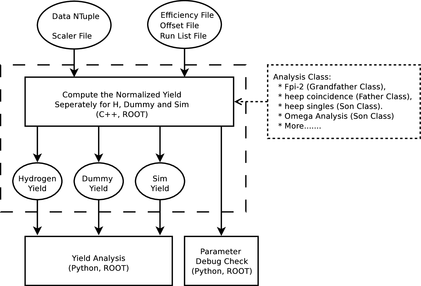
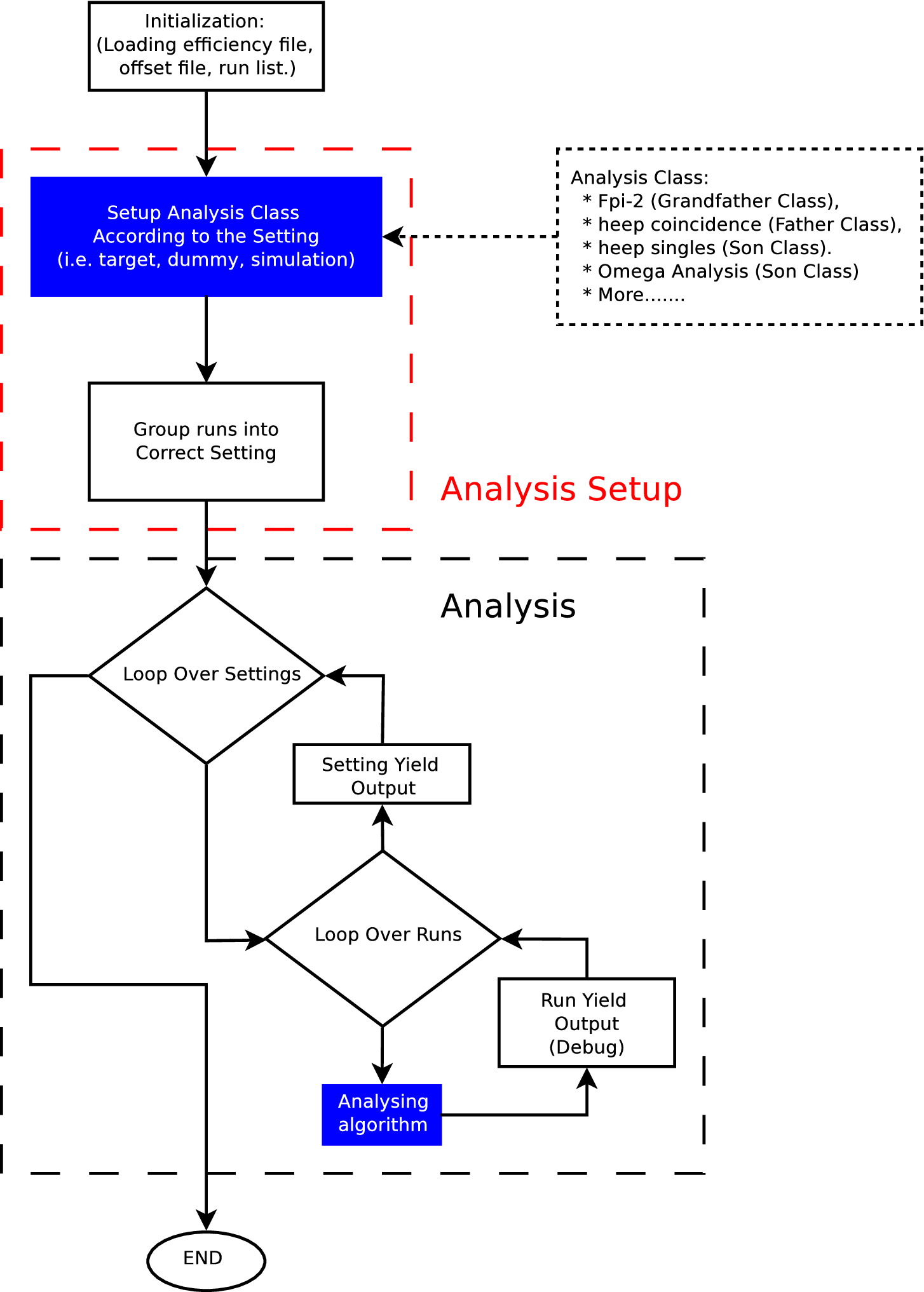
For the previous Fπ-2 analyses, the PAW code (for the yield computation) was inherited from the Fπ-1 [75] analysis. One of the major objectives of this work is to translate the FORTRAN based PAW code to a C++ based analysis platform, before extracting the yield. The new code is designed to use the libraries from ROOT [81], while maintaining the same functionality and algorithm structure.
Similar to the PAW macros, when computing the normalized experimental and Monte Carlo simulation yields, efficiency tables and offset files are needed as input as well as the data Ntuples. The computed yield and distributions (for cross-checking) are saved into a ROOT file. The schematics for computing the normalized yield are shown in Fig. 4.1. A small portion of the Fπ-2 data were used to test the new analysis platform and were compared with the PAW macro. The computed yields and cross-checking distributions (, , ,) agree 100%. Note that the C++ code takes one third of the time to run in comparison with the PAW code.
Fig. 4.2 shows the flow chart of the new C++ platform for extracting the normalized yield. In the analysis setup (red dashed box) section of the code, lists are created according to different experimental settings; here the experimental settings are categorized with respect to (virtual photon polarization), , and target type (hydrogen or dummy). Depending on the type of data analysis (Fπ-2, Heep singles, Heep coincidence), the number of settings can vary significantly. The constructor for each analysis class is initialized for each setting. The analysis class is specific to different types of analysis, where the earlier analysis class can be inherited and their functions can be used. The last part of the analysis setup is to loop over the data runs to associate each run with the correct efficiencies.
In the analysis (black dashed box) section of the code, the program will first loop over the setting list, then analyze each run in the list. The analysis (yield computation) takes into account the efficiencies, cuts and offsets on a run-by-run basis, and yields are accumulated over the setting. For debugging and cross-checking purposes, kinematic variables (, ), spectrometer acceptance parameters (, ) and absolute yield are saved to a ROOT file. After each setting ends, the yield sum and error from each run are normalized to 1 mC of beam charge. The normalized yield and yield error are saved, as well as the normalized distribution of kinematic variables and spectrometer acceptance parameters for the each settings.
For the simulation, the analysis procedure is much simpler since no particle identification (PID) cut is required. The efficiency files are replaced with a normalization factor file. Since SIMC generates events with unequal weighting, but uniform phase-space coverage, the normalization of the simulated data requires the additional weight applied to each event; the overall distribution needs an additional scale factor which is given by:
| (4.6) |
where the ‘normalization factor’ takes into account the luminosity () and simulated phase-space.
The coding philosophy is to maximize the customizability of the individual analysis while maintaining the standardized analysis setup procedure. For example, the differences in terms of the analysis codes for analysing the Fπ-2 test data and the Heep coincidence data are shown in the blue boxed region, where the main structure of the code remains identical.
In order to avoid repetitive coding, the earlier analysis classes such as Fπ-2 and heep_coin, can be directly inherited by any later class. Shared cuts and general utility functions can be easily accessed. It is the author’s hope that this code will be used to save time and effort by more and more students performing similar analysis. The final version of the code is located at the following GitHub22 2 https://github.com repository: https://github.com/billlee77/omega_analysis.
After the normalized yield for the hydrogen target, dummy target and simulation is computed and saved into a ROOT file, the experiment-simulation ratio is then generated by a python based script, as shown in Fig. 4.1. As a consistency check, the dummy target-subtracted distribution for all kinematic variables and acceptance parameters should not generate negative peaks.
From the flow chart given, one can develop a general structural picture regarding the iterative L/T separation procedure. The further details and justification regarding the iterative L/T separation procedure are given in Chap. 6.
Chapter 5 Heep Data Analysis
The elastic reaction 1H is often referred to as the Heep process. In this reaction, the recoil electrons are detected by the Short Orbit Spectrometer (SOS) and the protons are tracked by the High Momentum Spectrometer (HMS). Fig. 3.2 shows an overhead view of the standard Hall C experimental setup, which shows the SOS and HMS locations with respect to the target. These elastic scattering data provide a good check for the spectrometers, as well as various effects on reconstruction, such as radiative processes, multiple scattering and energy loss that were simulated by the Monte Carlo simulation (SIMC).
The data for the elastic 1H reaction were taken in four different kinematic settings, see Table 5.1. These kinematic conditions were modelled in SIMC, then compared to the data. For a detailed description regarding the cross section parameterization used for the Heep model, see Sec. 5.5.
During the Heep data runs, the data acquisition was operated in the coincidence mode for the 1H interaction. The coincident Heep study relies on the acceptance, tracking and PID information from both spectrometers to reconstruct variables such as missing mass, missing energy and . In addition, one can also perform the Heep study by examining only the recoil electron information in SOS (electron singles Heep mode) for cross checking purposes.
This coincidence Heep measurement almost replicates the exact experimental condition of the backward-angle production interaction: 1H. The coincidence trigger modes are identical between the two data sets. Furthermore, the event selection criteria and detector efficiencies used for both data sets are almost identical. Since the Heep data set has much less pion contamination than the data set, it is the optimal choice to study the proton detector efficiencies.
In this chapter, brief introductions on event selection criteria and background subtractions are given in Secs. 5.1 and 5.2. A variety of efficiencies specifically related to the proton selection in the HMS are described in Sec. 5.3. Finally, the simulation to experiment yield ratio (comparison) is presented in Sec. 5.6.
| GeV | GeV2 | GeV/c | deg | GeV/c | deg |
|---|---|---|---|---|---|
| 3.778 | 4.44 | 1.442 | 54.02 | 3.154 | 21.40 |
| 4.210 | 2.41 | 1.582 | 51.03 | 3.437 | 20.90 |
| 4.709 | 5.42 | 1.726 | 48.06 | 3.756 | 20.50 |
| 5.248 | 6.53 | 1.726 | 50.07 | 4.335 | 18.00 |
5.1 Data Selection and Correction
The first step in the identification of 1H events depends on the correct identification of electrons and protons in the SOS and HMS spectrometers, and on the precise coincidence timing information for the separation of the true and random coincidence events.
5.1.1 Particle Identification in SOS and HMS
In the SOS, due to its negative polarity setting, negatively charged pions are detected along with the recoil electrons. The pion contamination that was not rejected by correct coincidence time cut and cut, is less than 3 [55]. Electrons were detected and identified in the SOS using a combination of the Heavy Gas Cherenkov detector (HGC) and calorimeter. The HGC detector was used as a threshold detector with a mean SOS signal of 7 photo-electrons (pe) for one individual electron event. Good electron events were selected for number of pe threshold of N 0.5. A cut was also placed on the SOS calorimeter. In previous data analyses [55, 76], a threshold of 0.7 was in place, which is 99% efficient for selecting electrons.
In the HMS, where the proton events are selected, the background particles are pions and positrons. The rejection of the positrons is done via the signal from the Cherenkov detector. The positrons that were not rejected by the HMS pion trigger contribute 2.2% of all events with the correct coincidence timing and reconstructed missing mass. The limit of 0.5 photo-electrons in the Cherenkov detector provides positron rejection better than 99.5% [55]. The remaining positron contamination is negligible (much less than 0.1%). In addition, there is a nonzero probability for a proton to produce a knock-on electron ( radiation) while passing through the detector, which will result in a false signal. The contamination of the random electron-proton coincidence events that have the correct missing mass value is , and is sufficiently corrected by the random coincidence background subtraction (described in Sec.5.2.1). For documentation purpose, the complete set of particle identification (PID) cuts are given below:
- PID Cut:
-
&& && && &&
&&
5.1.2 Coincidence Timing vs.Particle Speed in the HMS


The most effective criterion for selecting the proton coincidence events is formed by examining the correlation between the relative particle velocity ratio (to the speed of light) inside of the HMS focal plane() versus the coincidence timing information. The particle velocity determined from the time of flight (TOF) information is generally an important element in the selection of events from the reaction of interest. The particle velocity in each spectrometer is calculated from the TOF information provided by the four scintillator element hodoscopes in the SOS and HMS. An example versus coincidence time distribution for the Heep data is plotted in Fig. 5.1.
Note that small offsets in the location of the blobs are observed (among data runs). For a given run, this offset is much smaller than the 2.1 ns timing window, therefore would not result any significant discrepancies. In this analysis, the blob positions have to be corrected on a run-by-run basis, before the versus distributions are summed over the same setting.
The HMS-SOS coincidence trigger TDC is timed by a HMS pre-trigger signal starting the TDC and stopped by a delayed SOS coincidence trigger signal. The time difference between the two triggers is the raw coincidence time. The raw coincidence time is corrected for time differences resulting from the variation in particle velocity and path distance traveled through each spectrometer. The difference in path length is estimated from the difference of the particle trajectory compared to the central trajectory. The corrected coincidence time allows for a resolution of 200 ps, which is sufficient to resolve the beam structure of the accelerator. Further details regarding the path length correction are given in Ref. [73].
From Fig. 5.1, a single ‘blob’ represents the coincidence proton events at ns. There is a ‘tail’-like structure (towards low ) attached to the blob and in addition there is a cluster of ‘zero’ events with . These ‘tail’ and ‘zero’ events are the effects due to the proton undergoing multiple scattering inside the scintillator material, HGC window and other material in their path inside of the HMS focal plane stack.
Fig. 5.2 shows the distribution for the zero () events. Note that the zero events contribute less than 3% of the random subtracted yield. 85% of the zero events are included by the real coincidence time window, as indicated by the red dashed lines, despite the fact that the most appropriate location of the coincidence window boundary may not correspond to the ns window from the location of the blob events. A vague correlation can be observed between the locations of the tail and zero events. Due to low statistical significance, the effect of the position of the real coincidence for the zero events has a negligible contribution (less than 0.4%) to the real experimental yield.
Based on further investigation, the ‘zero’ and ‘tail’ events have valid acceptance information (such as ), which can be treated as the ‘blob’ events. One of the possible causes for the ‘zero’ and ‘tail’ events are the interactions between proton and detector material downstream of the wire chamber. Since the detailed tracking and TOF information requires a fiducial cut on the hit location and signal strength from the hodoscopes, the deflected events due to multiple scattering can easily fail the fiducial cut and result an TOF overflow ().
During the data analysis, the ‘blob’ events correspond to , the ‘tail’ events have and the ‘zero’ events have .
5.1.3 Event Selection Criteria
The event selection criteria (cuts) used to analyze the Heep data are listed below, many of these conditions are similar to the ones used in the previous analysis efforts [55, 75, 76]. Note that the same cuts are used for the analysis.
- HMS Acceptance Cut:
-
&& && && .
- SOS Acceptance Cut:
-
&& && &&
&& . - Partial PID Cut:
-
&& && && && .
- ACD Threshold Cut:
-
Depending on the HMS central momentum setting, a different Aerogel Cherenkov threshold is required. See detail in Sec. 5.3.7.
- Full PID Cut:
-
Partial PID Cut && ACD Threshold Cut.
- Missing Mass () and Energy Cut ():
-
&& && .
Note that depending on the HMS central momentum setting, different ACD threshold cuts were applied, this is explained in detail in Sec. 5.3.7. The Full PID cut combines the Partial PID cut and ACD threshold cut. From this point onwards, unless specified, the term PID cut refers to the Full PID cut. Furthermore, a missing energy () cut of GeV and a missing mass cut were used. These cuts are further explained in Sec. 5.4.
5.2 Background Subtraction
The experimental data contain two types of non-physics background: random coincidences from unrelated electrons, pions, and protons in the two spectrometers, and coincident electrons and protons originating from the aluminum walls of the target cell. They are described in Secs. 5.2.1 and 5.2.2, respectively. Note that the same techniques were applied to the analysis.
5.2.1 Random Coincidence Background Subtraction
Random - coincidence events constitute a background and have to be subtracted from the data sample. The estimation of the random background includes two separate random windows, one before and one after the real - window. The ‘early’ random coincidence window (blue boxes right side of proton blob) was 6.3 ns wide (three times the real window), and the ‘late’ random coincidence window (magenta boxes left side of the real peak) was 2.1 ns wide (one real window). The real - peak is avoided in the placement of random coincidence cuts. The number of random events within the real window can be estimated as the total of random events over the number of the random windows (four random windows), and it is subtracted from the total number of events in the real window.
5.2.2 Cell Wall Contribution and Dummy Target Data Subtraction
Another type of background that needs to be removed from the sample of good events is the background due to the scattering from the aluminum target cell walls enclosing the liquid hydrogen. The target cell wall contributes a relatively small percentage of the total yield (2-4.5%).
The target cell wall contribution to the background events can be estimated by taking dummy target data and subtracting them from the data with the LH2 target. The dummy target consists of two aluminum foils 4 cm apart and centered at the target station. Note that the dummy target is intentionally made thicker, thus maxing the yield while minimizing the run time. Fig. 5.3 shows the distribution for the LH2 target for the = 2.45 GeV2 setting in black dots and the cell wall contribution in green. Since the SOS angle is 50∘ with respect to the electron beam, the separation between the two green bumps is not 4 cm.
The dummy target data are analyzed in the same way as the regular data, including the same method of random coincidence subtraction and applying the same event selection criteria (cuts). The extracted experimental yields (number of events which pass the event selection criteria) are then subtracted from the real data yields, taking into account the additional weight of 7.022 to account for the difference in wall thickness between target cell and dummy target. When compared to other experimental uncertainties, the uncertainty in the target thickness ratio between target cell wall and dummy target is negligible.

5.3 Efficiency Study
5.3.1 Analysis Information
In computing the normalized yield, one must apply corrections for inefficiencies such as trigger, track reconstruction and data acquisition deadtime. The total experimental yield can be written as
| (5.1) |
where is the total number of selected good events, is the efficiency correction factor (all detector efficiencies and electronic live times combined) and is the total accumulated electron beam charge. Details regarding efficiency studies, such as event tracking efficiencies and electronic live time, are documented in this section. These efficiencies are also applied to the analysis.
Note that the analysis presented in this thesis does not include the raw data replay (calibration and conversion). The - data ntuples used were created during the Fπ-2- analysis by T. Horn [55].
5.3.2 Computer and Electronic Live Time
The data acquisition (DAQ) system efficiency for experiments is rarely perfect (100%). During the experiment, the DAQ which consists of electronics and computers, has a number of rate-dependent efficiencies (live time) due to their processing speed and the level of the logic complexity. These rate-dependent efficiencies need to be carefully studied in order to obtain an accurate absolute physics measurement.
The computer live time (CLT) can be calculated from the ratio between the recorded events and total events (triggers). The DAQ system used during Fπ-2 recorded data on a single-event basis, meaning once the recording process was initiated, no more event could be recorded until the first event processing is completed. This would inevitably cause event loss at high event rate. Note that there is also an efficiency associated with the performance of the trigger supervisor, whose effect is negligible when compared to the CLT.
| Run | PS1 | BoT | hS1X | ||||||
| Production Runs | |||||||||
| 47055 | 1300 | 82386 | 46476348 | 1108.5 | 143246000 | 39774 | 0.9646 | 0.9926 | 0.9973 |
| 47056 | 1300 | 33544 | 18895112 | 448.5 | 58256076 | 16225 | 0.9643 | 0.9926 | 0.9973 |
| 47057 | 4000 | 26115 | 19616695 | 475.5 | 60404320 | 16775 | 0.9676 | 0.9944 | 0.9973 |
| 47062 | 4000 | 137852 | 103301496 | 2485.5 | 318552993 | 88744 | 0.9662 | 0.9939 | 0.9974 |
| Carbon Data Runs | |||||||||
| 47012 | 700 | 360222 | 204144117 | 1106.5 | 279010493 | 5 | 0.9655 | 0.9671 | 0.9879 |
| 47017 | 300 | 351032 | 90054730 | 608.5 | 123248274 | 2 | 0.9000 | 0.9425 | 0.9903 |
| 47018 | 200 | 369808 | 63678174 | 600.5 | 87321171 | 1 | 0.8696 | 0.9394 | 0.9931 |
| 47023 | 200 | 377130 | 58634905 | 923.5 | 80547701 | 0 | 0.8919 | 0.9607 | 0.9959 |
| Heep Runs | |||||||||
| 47049 | 1 | 1000087 | 882351 | 1167.5 | 38251650 | 4833 | 0.9615 | 0.9254 | 0.9999 |
| 47050 | 1 | 1002450 | 882596 | 1183.5 | 38263209 | 4915 | 0.9618 | 0.9268 | 0.9999 |
| 47051 | 1 | 1000300 | 881914 | 1152.3 | 38243611 | 4817 | 0.9624 | 0.9264 | 0.9999 |
| 47054 | 100 | 855628 | 747156 | 784.5 | 34215154 | 366 | 0.9638 | 0.9072 | 0.9999 |
| Run | PS2 | BoT | sS1X | ||||||
| Production Runs | |||||||||
| 47055 | 1100 | 82386 | 7931280 | 1108.5 | 53758202 | 39774 | 0.9926 | 0.9924 | 0.9991 |
| 47056 | 1100 | 33544 | 3219778 | 448.5 | 21869817 | 16225 | 0.9961 | 0.9924 | 0.9991 |
| 47057 | 750 | 26115 | 3361715 | 475.5 | 22677390 | 16775 | 0.9955 | 0.9941 | 0.9991 |
| 47059 | 750 | 31564 | 4049601 | 562.5 | 27328976 | 20347 | 0.9907 | 0.9941 | 0.9991 |
| Carbon Data Runs | |||||||||
| 47012 | 300 | 360222 | 23832512 | 1106.5 | 166164337 | 5 | 0.9925 | 0.9665 | 0.9982 |
| 47017 | 150 | 351032 | 10578904 | 608.5 | 73265713 | 2 | 0.9882 | 0.9413 | 0.9985 |
| 47018 | 100 | 369808 | 7408278 | 600.5 | 51820714 | 1 | 0.9890 | 0.9381 | 0.9990 |
| 47023 | 70 | 377130 | 6918378 | 923.5 | 47723650 | 0 | 0.9904 | 0.9594 | 0.9993 |
| Heep Runs | |||||||||
| 47049 | 1 | 1000087 | 203454 | 1167.5 | 18730307 | 4833 | 0.9939 | 0.9261 | 1.00 |
| 47050 | 1 | 1002450 | 203584 | 1183.5 | 18717954 | 4915 | 0.9949 | 0.9266 | 1.00 |
| 47051 | 1 | 1000300 | 202534 | 1152.3 | 18711655 | 4817 | 0.9935 | 0.9254 | 1.00 |
| 47052 | 1 | 556253 | 112095 | 668.5 | 10388704 | 2682 | 0.9940 | 0.9269 | 1.00 |
The probability of events occurring in an interval for a certain event rate can be described by the Poisson distribution:
| (5.2) |
The probability of zero events occurring in the interval is thus
| (5.3) |
For small , the probability can be estimated as . In this analysis, is the live time, is the event rate and is the time needed to process one event (computer or electronic processing time).
In this section, the studies of the CLT and electronic live time (ELT) as functions of event rate are presented. The data runs used to perform both studies include: LH2 target production runs, carbon target luminosity runs and - elastic scattering (Heep) runs. Note that carbon runs are selected to extend the event range, since Heep and runs have relatively low event rate. Four data run examples were selected from each data type and are listed in Table 5.3. The actual correction applied was determined by using the scaler information of each run. Eqn. 5.3 was only used to check for consistency, to be sure the live time values make sense.
5.3.2.1 Electronic Live Time


The electronic dead time (EDT) is normally estimated by observing the variation on pre-trigger scaler counts of various gate widths. Apart from the pre-trigger (PRE), there are PRE50, PRE100, PRE150 and PRE200 scalers corresponding to pre-trigger gate widths of 40 ns, 100 ns, 150 ns and 200 ns. Note that the PRE gate width is around 60 ns. PRE50 is intentionally set to be 40 ns to help understand the relationship between EDT and the pre-trigger gate width.
The real number of pre-triggers is calculated as
| (5.4) |
where is the measured pre-trigger scaler counts with 60 ns gate width; is the pre-trigger correction computed by the pre-trigger scaler counts of other gate widths, i.e. 40 ns and 100 ns. Since the EDT is expected to scale linearly with the gate width, there are a number of ways to compute the :
| (5.5) |
where , and are pre-trigger scaler counts of PRE50, PRE100 and PRE150, respectively. An additional factor of 6/5 is needed as the gate width difference between PRE100 and PRE150 is only 50 ns instead of 60 ns. The chosen methodology in this analysis involves PRE100 and PRE150 to compute .
The EDT can be calculated as
| (5.6) |
where the approximation = , where corresponds to the actual number of events collected during the experiment since the coincidence ggate width is set to 100 ns. Thus, ELT is given by
| (5.7) |
and its uncertainty
| (5.8) |
Note the equation of assumes binomial statistics due to the fact that EDT values are very close to zero. The function form of the binomial statistics is different from the standard Poison statistics.
The HMS and SOS ELT versus the pre-trigger rate are plotted separately in Fig. 5.4. The fitting results suggest a time constant 67 0.15 ns for the HMS and 77 4 ns for SOS. These values differed slightly from the previously reported time constants during the Fπ-2 studies: 63.9 ns and 72.5 ns [55]. The differences might be contributed by two major sources: 1) Different data runs were used for this and the previous study; 2) In this study, since all data points from the production, Heep and carbon luminosity runs were included, therefore the number of data points was significantly more than the previous ELT study. The ELT time constants extracted from this study are accurate, since they were obtained directly from the production data.
5.3.2.2 Computer Live Time
Fig. 5.6 shows the CLT versus All Trigger Rate (ATR). All Trigger ( from Table 5.3) is the total number of triggers over HMS, SOS singles and coincidences, which can be calculated as:
| (5.9) |
where and are the number of HMS and SOS single arm pre-triggers; PS1 and PS2 are the HMS and SOS singles pre-scale factors, and PS3 is the HMS+SOS coincidence pre-scale factor, which is typically set PS3=1; the ATR is calculated as
| (5.10) |
where BoT is the beam on target time.
The data points in Fig. 5.6 are from production, Heep and carbon target luminosity runs. The fitting curve only takes into account the data points from the production runs, and yields a CLT time constant of: = 0.172 0.003 ms. It seems that the Heep data points are spread much wider in rate than those of the data for both HMS and SOS, and the Heep spread subsequently forms two (top and bottom) trails. It suggests that there may exist more than one effective value for the CLT constant.

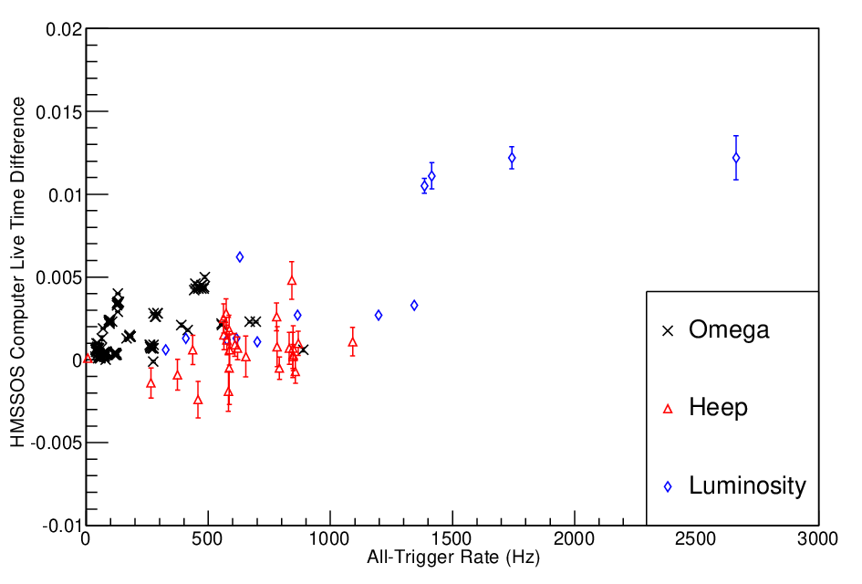
Since there was only one data acquisition computer for both spectrometers, the CLT for HMS and SOS should be identical within statistical uncertainties. However, a small deviation is observed and the difference (HMSSOS) is shown in Fig. 5.6. The difference seems to form a increasing trend as the all trigger rate increases; the CLT difference for Heep and is within 0.5%.
To study further the CLT at low rate, the HMS and SOS CLT versus ATR are plotted separately in Fig. 5.7 with Heep and runs. The Heep data seems to split into top-bottom trails similar to Fig. 5.6.
Besides the small difference between HMS and SOS CLT, a difference is observed in the fitted HMS and SOS CLT time constants as shown in Fig. 5.7. Note that only the production runs are used to extract the values, since these data scatter much less. The extracted HMS = 0.168 0.004 ms and SOS = 0.175 0.004 ms, where the combined HMS and SOS CLT time constant from Fig. 5.6 is = 0.172 0.004 ms.
The CLT was previously reported as = 0.49 ms from the Fπ-1 data analysis [75], which suggests the computer processing speed for Fπ-2 is 3.5 times faster than that for Fπ-1, due to DAQ upgrades that occurred between Fπ-1 and Fπ-2.
Runs #47141 and #47183 are identified as bad runs. The relevant information are listed in Table 5.4. Both runs have large HMS pre-trigger number (10 higher than runs with similar Beam On Time) and over 90% computer dead time.
Note that the purpose of this analysis is to understand the trends of the CLT; the applied rate dependent correction to the experimental data used the actual efficiency value determined for each run.


| = 2.45 GeV2, = 2.21 GeV, = 4.21 GeV, = 0.27 | ||||||||||||
| Run | PS1 | BoT | hS1X | |||||||||
| 47141 | 3000 | 150902 | 4397010598 | 3510.5 | 343335387 | 84215 | 0.9536 | 0.9551 | 0.9548 | 0.9549 | 0.0231 | 0.9982 |
| 47183 | 3000 | 142913 | 4386158993 | 3212.5 | 306009605 | 80627 | 0.9476 | 0.9489 | 0.9495 | 0.9486 | 0.0207 | 0.9982 |
5.3.3 Spectrometer Tracking Efficiencies
The tracking efficiency is defined as the probability that a particle, identified as an electron or proton, is associated with a valid track from the wire chambers.
In the HMS spectrometer, an good proton event is determined if it satisfies the proton identification criterion. The HMS proton PID criterion requires signals in at least three of the four hodoscope planes (a valid SCIN signal, see Sec. 3.7), in addition to the PID information from TOF, both HGC and ACD detectors, and the calorimeter (with the fiducial and EM shower cuts). Except for the = 6.52 GeV2 Heep setting (proton momentum exceeds ACD threshold momentum), the proton momentum is below the threshold for generating the Cherenkov radiation in both HGC and ACD, therefore absence of signal or sub-threshold signals (from both Cherenkov detectors) are expected.
For the electron selection in the SOS, the similar levels of information are required (such as a valid SCIN signal) by the electron identification criterion. The electrons are expected to generate an over-threshold signal in the SOS HGC, an EM shower in the calorimetry and velocity much closer to the speed of light.
The failure of the tracking algorithm to identify a valid event can be caused by a wire chamber inefficiency, or a failure of the tracking algorithm itself. While the raw data are processed, the replay engine keeps count of the number of events for a given type with, and without, a track.
The scaler output from the data analysis engine generally includes several tracking efficiencies for different particle types at different thresholds and trigger conditions.
Carbon target luminosity runs are excluded from this study. Since luminosity runs have few coincidence triggers, the corresponding coincidence tracking efficiencies are unavailable. Also, the HMS was configured to operate with negative polarity during the carbon target luminosity runs, therefore no proton events are expected at the wire chamber.
5.3.3.1 Choice of HMS Tracking Efficiency


There were four sets of tracking efficiencies generated by the replay engine and stored in the HMS scaler files:
- P SING FID TRACK EFFI ()
-
Proton tracking efficiency for HMS singles events. Protons were selected by ACD cut less than 4 pe and a HGC cut less than 0.5 pe.
Cut limits: && .
- P SING FID TRACK CTRIG ()
-
Proton tracking efficiency for HMS+SOS singles and coincidence events. Protons were selected by the same ACD and HGC cuts. Note that, despite the name (‘CTRIG’), there was no cut on the coincidence trigger.
Cut limits: && && .
- P SING FID TRACK CAL_CUT ()
-
Proton tracking efficiency for HMS singles events. Protons were selected with the same ACD and HGC cuts, in addition to lower and upper limits on the energy deposited in the calorimeter.
Cut limits: && && && .
- P SING FID TRACK CTRIG CAL_CUT ()
-
Proton tracking efficiency for HMS singles. Protons were selected with the same ACD and HGC cuts, in addition to lower and upper limits on the energy deposited in the calorimeter. The cut on calorimeter is tighter than that of P SING FID TRACK CAL_CUT.
Cut limits: && && && .
Note that a fiducial cut on the spectrometer focal plane is applied to all four sets of efficiencies to reject events which come close to the edges of the focal plane.
Fig.5.9 shows all four tracking efficiencies versus the HMS S1X hodoscope plane (hS1X) rate. The differences between all sets of tracking efficiencies are surprisingly small, especially for event rate 100 kHz. The differences at low event rate are more substantial, however, the error bars are also dramatically larger. As to be explained in Sec. 5.3.4, the selected HMS tracking efficiencies will be corrected using Eqn. 5.12. Fig.5.9 shows the P SING FID TRACK CAL_CUT and its corrected value.
P SING FID TRACK CAL CUT was selected for the Heep and analyses for the following reasons:
- •
is the only tracking efficiency that requires a “positive” signal in PID detectors, thus eliminating “junk” hits. also has the same condition, but the cut appears to be too aggressive (over constraint) [61],
- •
- •
was used as HMS tracking efficiency during the Fπ-2- analysis.
Further information regarding on the choice of the tracking efficiency is documented in Ref. [82].
5.3.3.2 Choice of SOS Tracking Efficiency

For electron tracking inside the SOS, there are also four tracking efficiencies from the SOS scaler files can be used to perform the data analysis as listed below:
- SING TRACK EFF
-
Tracking efficiency for all SOS singles events including pion, hadron and electron events,
- E SING TRACK EFF
-
Electron tracking efficiency for SOS singles events,
- CLEAN COIN TRACK EFF
-
Tracking efficiency for all clean HMS+SOS coincidence pion, hadron and electron events,
- E COIN TRACK EFF
-
Electron tracking efficiencies for HMS+SOS coincidence events.
Fig.5.10 shows all four tracking efficiencies versus the SOS sS1X rate. Data points for SING TRACK EFF and CLEAN COIN TRACK EFF show a surprising amount of scatter, particularly for sS1X rate below 100 kHz. E SING TRACK EFF and E COIN TRACK EFF seem to be consistently following a linear relation with the rate. The average difference between the two sets of efficiencies is around 0.5%. The error bars for both sets of efficiencies are around 0.2-0.4% below 100 kHz and less than 0.2% above 100 kHz. E SING TRACK EFF was selected for the Heep and analyses, since it has higher statistics. There is no additional correction applied to the SOS tracking efficiency due to its lower event rate (compared to the HMS rate) during the data taking, which implies the SOS tracking efficiency is not so sensitive to the rate.
5.3.4 Carbon Target Rate Study
In theory, physical observables (measurements) such as differential cross-section should not depend on the luminosity. In reality, detector efficiencies are often affected by high event rates which will directly influence the experimental results.
Particular to the L/T separation studies, two separate measurements are required at two different beam energies. Due to the difference in scattering cross sections and experimental acceptances, the event rate for low beam energy setting can be dramatically different from the rate for the high beam energy setting. In order to accurately correct the rate dependence in the measured experimental data, it is critical to carefully study the relationship between the overall HMS efficiency versus event rate. The standard technique is to take deep inelastic scattering measurements using a carbon target at a range of electron beam currents.
In the HMS spectrometer, the charged particle trajectories are measured by two drift chambers, each with six planes of wires, as described in Sec. 3.6.1. Note that a “good track” requires 5 out of 6 wire planes to fire in each drift chamber for both spectrometers. The effectiveness of the overall tracking algorithm in the software analyzer is expected to have a rate dependence, as the detection efficiency and multiplicity drop with rate. The tracking algorithm is capable of taking into account multiple track events, which are more probable at high rate.
There are two separate methods to calculate the spectrometer tracking efficiency with the same tracking algorithm. The Fπ-1 method [76] (which is the default method for the data analyzer) and the Fπ-2- method [55].
Comparing to the Fπ-2- method [76], the Fπ-1 method applies additional fiducial cuts on the scintillator planes. In the case of multiple track events, these cuts place a bias on the event sample used to calculate the HMS tracking efficiency. Since 2-track events have lower efficiencies than 1-track events, the resulting bias caused the tracking efficiencies to be overestimated. The experience from the Fπ-1 experiment [76] has suggested the HMS normalized yield from carbon target (for electrons) computed using the Fπ-1 method efficiencies fall linearly with rates, due to the presence of multiple track events in the drift chambers at high rate environment and particles hitting near the edge of the wire chambers that fail the fiducial cuts. This observation implies the tracking efficiency can not adequately correct the rate dependent effect in the tracking algorithm and an additional (linear) correction was required.
At low rate ( kHz), the tracking efficiency computed using the Fπ-2- method shows no additional dependence on rates [55, 76]. However, the tracking efficiency is determined to be unreliable at a high rate environment ( kHz) [76] due to the looser event selection used (demonstrated during the Fπ-2- analysis [76]).
In the analysis, the Fπ-1 [75] method is used due to its greater reliability over a wider range of rates. Therefore, an additional rate dependent correction on the tracking efficiency study is required. A similar approach was successfully used in the Fπ-2- analysis [76].
In order to rigorously study the tracking efficiency, a study of yields from carbon target versus rate was performed. The study requires the extraction of the inclusive experimental yields, plotted against the trigger rate of the first hodoscope plane for the HMS (hS1X). The single arm experimental yield () is calculated as
| (5.11) |
where is the number of electrons obtained using a loose cut to the ntuples; is the HMS singles pre-scale factor applied during the data acquisition; is the accumulated electron beam charge; is the Electronic Live Time (ELT); is the Computer Live Time (CLT); is the tracking efficiency obtained using the scaler information (from the data replay using the F-1 tracking efficiency computation method). Note that all scaler information except came from the Fπ-2- replay, since it uses the Fπ-2 method to compute the tracking efficiency.
The scaler information for all the carbon luminosity runs are listed in Table 5.5. is listed as SING in the table. refers to the number of events passed the selection criteria after applying a loose cut to various parameters, and the actual cuts are listed below,
- Event selection criteria:
-
&& &&
&& && && .
| Run | hELCLEAN | hS1X | BoT | hS1X/BoT | PS1 | SING | ||||
| = 4.210 GeV, =12.00∘, =3.000 GeV/c | ||||||||||
| 47012 | 100809 | 181614321 | 279010493 | 1106.5 | 252 kHz | 700 | 0.9797 | 0.9671 | 0.9879 | 165047 |
| 47017 | 44330 | 80184449 | 123248274 | 608.5 | 202 kHz | 300 | 0.9810 | 0.9425 | 0.9903 | 166750 |
| 47018 | 31249 | 56737629 | 87321171 | 600.5 | 145 kHz | 200 | 0.9815 | 0.9394 | 0.9931 | 176610 |
| 47023 | 28692 | 52272440 | 80547701 | 923.5 | 87 kHz | 200 | 0.9834 | 0.9607 | 0.9959 | 167320 |
| = 4.702 GeV, =10.57∘, =4.050 GeV/c | ||||||||||
| 47757 | 42974 | 233316130 | 303675199 | 575.5 | 527 kHz | 500 | 0.9743 | 0.6415 | 0.9705 | 222339 |
| 47759 | 124775 | 675461151 | 880596706 | 1590.5 | 553 kHz | 2000 | 0.9742 | 0.8738 | 0.9700 | 219433 |
| 47760 | 19126 | 107791771 | 138777445 | 710.5 | 195 kHz | 250 | 0.9807 | 0.7171 | 0.9896 | 232082 |
| 47763 | 56962 | 308207310 | 402136284 | 724.5 | 555 kHz | 750 | 0.9749 | 0.7225 | 0.9699 | 220876 |
| 47764 | 29473 | 159412019 | 208067731 | 376.5 | 552 kHz | 250 | 0.9746 | 0.4685 | 0.9701 | 222754 |


The experimental yields were computed using Eqn. 5.11 and information from Table 5.5, then normalized to unity at hS1X rate of 0 Hz. The normalized yields versus hS1X rate are plotted in Fig. 5.12. The error bars include the statistical uncertainty and an estimated systematic uncertainty of 0.3% [76] added in quadrature, to take into account beam steering on the target and other sensitive effects. Data from the two kinematic settings were separately fit versus rate (blue and red curves in the figure), and they are combined to yield the black curve.
The reason for the rate dependent tracking efficiency correction has been given in the earlier text, and the tracking efficiency correction as a function of rate is given by
| (5.12) |
Fig. 5.12 shows the corrected normalized yields plotted against the beam current. The fitting result seems to be consistent with 0 within the 1 error band (dashed line). This confirms that the converted efficiencies now have the correct dependence on event rate, which will produce a normalized yield that is independent of luminosity.
Furthermore, carbon luminosity data runs #47758 and #47761 are not used for the target study since their normalized yields are dramatically far away from the fitted slope.
5.3.5 LH2 Target Boiling Study

When the electron beam hits the liquid cryogenic target, the energy deposit is equivalent to a 100 Watt bulb (based on the estimation from Sec. 3.5) across a small area. This consequently induces localized density fluctuation often referred to as “target boiling”, more detail was given in Sec. 3.5. In order to minimize the target density fluctuations, the beam was rastered over an area of mm2, rather than being focussed to a single point on the cryotarget. The target boiling effect can be measured by comparing the yields at fixed kinematics and varied beam current.
The Fπ-2 measurement used the “tuna can” cryotarget geometry and circular beam raster design, which are expected to result in boiling corrections 1% due to better flow of the cryogenic fluids. In order to make sure the LH2 target boiling contributes no additional dependence to the normalized yields, the LH2 target study was repeated and compared with the previous LH2 target studies [76].
| Run | hELCLEAN | hS1X | BoT | hS1X/BoT | PS1 | SING | |||||
| = 4.210 GeV, =12.00∘, =3.000 GeV/c | |||||||||||
| 47010 | 55703 | 219259338 | 346569464 | 606.5 | 571kHz | 700.0 | 0.9738 | 0.9394 | 0.9268 | 0.9724 | 183051 |
| 47014 | 37921 | 150584896 | 238130720 | 520.5 | 457kHz | 300.0 | 0.9762 | 0.9485 | 0.8765 | 0.9781 | 279893 |
| 47019 | 15462 | 61940123 | 98109699 | 304.5 | 322kHz | 200.0 | 0.9792 | 0.9595 | 0.8638 | 0.9846 | 171455 |
| 47022 | 13647 | 55126254 | 87477847 | 442.5 | 197kHz | 200.0 | 0.9812 | 0.9691 | 0.9145 | 0.9907 | 162904 |
The information for the LH2 target study runs are listed in Table 5.6. The cuts of
- Event selection criteria:
-
&& && && ,
are applied to the data Ntuples for each of these runs to extract the number of events that passed the selection selection criteria (SING).
The experimental yields were calculated using Eqns. 5.11 and 5.12. The normalized yields are plotted versus current in Fig. 5.13. The error bars include statistical uncertainties and an estimated systematic uncertainty of 0.3% is added in quadrature. The fitting curve is consistent with 0 across the measured beam current range, thus confirming no additional correction is needed for the effect of target boiling. This is consistent with the study presented in Ref. [55].
5.3.6 SOS Coincidence Blocking


A coincidence event will normally be started at the TDC with a delayed HMS trigger and stopped by the SOS trigger. Due to interference between random coincidence and real coincidence events, a fraction of events are recorded with the coincidence time outside the main timing window, as defined by the pre-trigger signal width. The “coincidence blocking” events will be lost from the data due to the coincidence time cuts used in the analysis, therefore a study is needed to correct for data loss. The and Heep data are used for this study.
Examples for the coincidence time spectra of and Heep data runs are shown in Fig. 5.14. The main coincidence window corresponds to the region between TDC channel 1186 to 2240 for runs and 1756 to 1910 for Heep runs. The conversion between picoseconds and TDC channels is approximately 120 ps per channel. The events left of the main timing windows are the coincidence blocking events due to the SOS singles triggers arriving earlier than the SOS coincidence trigger. Thus, the TDC is stopped too early, and the resulting events fall outside of the main coincidence time window (early triggers). Note that due to the trigger setup (started by the HMS pre-trigger and stop by the SOS pre-trigger), there is no early HMS event therefore no need for the coincidence correction.

The coincidence blocking correction can be estimated from the rate dependence of the number of blocked events, similar to the deadtime correction in Sec. 5.3.2. The comparison of the number of events outside of the main coincidence time window, and the total number of events, yields the coincidence blocking rate:
| (5.13) |
where is the number of “early” SOS events (triggers) in the measured coincidence time spectrum and the is the total number of events independent of the coincidence time. The good coincidence rate takes into account events within the main coincidence time window, and can be written as a function of the coincidence blocking constant ,
| (5.14) |
where is the SOS pre-trigger rate. Binomial statistics are used to calculate the uncertainty for the good coincidence rate [83]
| (5.15) |
Fig. 5.15 shows the SOS blocking correction plot, where the good coincidence rate is plotted as a function of SOS pre-trigger rate. From the fitting result, the coincidence blocking time constant () in Eqn. 5.14 is determined, 103.580.43 ns.
From the Fπ-2- analysis [55], the constant was reported as ns [55]. The difference between two values, is due to different data set used for each studies. In the (this) analysis, the study only includes the data set which is a small subset of the Fπ-2- data. The previous coincidence blocking study included the whole data set.
This Eqn. 5.14 with newly determined constant was applied to the data as the Cherenkov coincidence correction.
5.3.7 HMS Aerogel Cherenkov Detector Threshold Cuts
| Inter. Cor. | Data Set | haero_su Cut | ||||
| GeV2 | GeV/c | % | % | % | pe | |
| 2.41 | 3.44 | 54.14 | 80 | 4.58 | Heep | |
| 4.42 | 3.15 | 50.82 | 80 | 4.36 | Heep | |
| 5.42 | 3.76 | 56.82 | 80 | 4.75 | Heep | |
| 6.53 | 4.34 | 62.89 | 80 | 5.15 | Heep | |
| 1.60 | 2.93 | 37.77 | 80 | 3.51 | ||
| 2.45 | 3.33 | 70.65 | 80 | 5.65 |


During the Fπ-2 experiment, the primary objective of the ACD was to perform a clean separation; see Sec. 3.6.5 for further detail regarding the ACD.
Table 5.7 shows the HMS central momentum values (), ACD cuts and other relevant information for four Heep settings and two settings. For the Heep data, ACD cuts were used to exclude events beyond the applied threshold. For the data, ACD cuts were used to ensure selections of clean coincidence proton events, while events beyond the cuts were corrected by an ACD cut efficiency factor (described in Sec. 5.3.8).
The HMS ACD cuts for the Heep data were determined using the HMS ACD () distributions (logarithmic scale), shown in Fig. 5.16. The red boundary lines were drawn as the distributions started to plateau.
The =2.41 GeV2 Heep setting is a sub-threshold HMS central momentum setting, however, its ACD distribution (see Fig.5.16(a)) is unusually wide, which may be due to mis-calibration; an cut of is applied. The = 6.53 GeV2 Heep setting has a HMS central momentum of 4.34 GeV/c that is above the Cherenkov radiation threshold momentum for a proton, and its ACD distribution seems to allow the same cut of as the other two well-calibrated sub-threshold settings.
5.3.8 HMS ACD Cut Study for the Analysis


Unlike the Heep runs, the data have a much higher rate of pion contamination in the coincidence trigger that requires both the - cut and the HMS ACD cut () to cleanly select the proton coincidence events.
The - distribution for Heep data in Fig. 5.19(b) shows only the prompt proton coincidence bunch with scattered random coincidence events. The - distribution for the data looks dramatically different, where the separate and coincidence bunches are visible (described in Sec. 6.3.1). Since have a higher velocity due to its lighter mass (at the nominal HMS momentum), it arrives the at HMS detector package (hodoscopes) 4-5 ns earlier. Thus, by applying the - cut, the main proton bunch can be separated from the pions.
Fig. 5.17(a) and (b) show the distributions without, and with, the - cut, respectively. The red boundary indicates the HMS ACD cut of pe. Both distributions have the same acceptance and PID cuts. (b) is normalized (to 1 mC of beam charge) and random coincidence contribution has been subtracted, where (a) is not. Fig. 5.17(b) is visually clean, 90.9% the events are within the cut region (red boundary). Beyond the pe limit, the tail contains predominantly proton events with a small contamination in the tail region ( pe), since the spectrometer setting is optimized for detection. The level of pion contamination is difficult to estimate, since coincidence proton events beyond the haero_su cut cannot be accurately counted.
As indicated in Sec. 5.3.7, the Heep data have much less pion contamination than the data. Thus, two sub-threshold (HMS ACD) Heep settings were used to estimate the proton coincidence events beyond the cut ( pe). The ACD distributions of Heep settings of =4.42 and 5.42 GeV2 are plotted in Fig. 5.18(a) and (b). The cut efficiency is the ratio between events within the red boundary and the total. The averaged efficiency between the two Heep settings is 92.71.2%; the normalized experimental yield will be divided by this efficiency for the analysis. Since very few coincidence proton events from the dummy target are able to survive the Heep analysis cuts, the contributions from the Dummy target runs are negligible.
For the pion contamination within the cut boundary, the random subtraction process is sufficient assuming the random proton and contamination is identical for each bunch; therefore, no additional correction is necessary.
5.3.9 hsbeta Distribution and Proton Interaction Correction

By taking a closer look at the distribution and the versus spectrum in Fig. 5.19, a cluster of ‘zero’ events () can be seen. After performing studies, such as those described in Sec. 5.1.1, and through private communication with Hall C experts [61], the ‘zero’ events have been included along with ‘tail’ () and ‘blob’ () events for the Heep and analysis. In addition, a proton interaction correction study is performed using the same methodology used for determining the pion absorption correction during Fπ-2- analysis [76].
Note that in the Fπ-2- analysis, the ‘tail’ events were corrected by a correction factor, whereas both ‘zero’ and ‘tail’ events are included in the yield computation for the Heep and analysis.
From a recoil proton (from the target chamber) traversing through the HMS entrance window, to the generation of a valid trigger, a proton can interact with a variety of detector materials along its path through the spectrometer.
The dominant proton reaction for the recoil protons is inelastic scattering (mainly pion production), elastic and (quasi) elastic scattering (with heavier elements than 1H). In the case of pion production and (quasi) elastic scattering, a secondary pion, proton or neutron is emitted along the path of the recoil proton momentum, therefore has a probability to generate a valid trigger. From Table 5.7, the mean value of the HMS central momentum settings is 3.5 GeV/c. The and total cross sections are dependent on the proton momentum, and are estimated to be 43 mb at 3.5 GeV/c [1], where the elastic cross section is 1/3 of the total cross section. The proportion of protons lost due to these interactions must be correctly accounted for.
The situation is complicated by the fact that the proton interaction in the scintillators, ACD and HGC detector material leading to the emission of energetic nucleons can generate valid triggers or tracks. These events are part of the distribution and are already included in the analysis. Subsequently, if one applies a simple proton transmission correction based on the scattering cross section and material properties, it would result in an overcorrection. The proton interaction correction study is intended to account for the HMS triggers that are lost due to proton interactions in the material upstream of the drift chambers, or interaction in the detector stack, such as large angle deflection or leading to the emission of low momentum nucleons, which do not give enough signal in the scintillators providing a valid trigger.
| Absorber | Material | Partial Sums | |||||
|---|---|---|---|---|---|---|---|
| cm | g/cm3 | g/cm2 | g/cm2 | % | % | ||
| Target | LH2 | 1984 | 0.072 | 43.3 | 0.143 | 0.370 | |
| Target Window | Al | 0.013 | 2.700 | 70.6 | 0.035 | 0.056 | |
| Chamber Window | Al | 0.0406 | 2.700 | 70.6 | 0.110 | 0.174 | |
| Chamber Gap | Air | 15 | 0.001 | 62.0 | 0.018 | 0.033 | |
| Entrance Window | Kevlar | 0.0381 | 0.740 | 60.0 | 0.028 | 0.052 | |
| Idem | Mylar | 0.0127 | 1.390 | 60.2 | 0.017 | 0.032 | |
| Exit Window | Titanium | 0.0508 | 4.540 | 79.9 | 0.231 | 0.324 | |
| Target - Exit Window Sum | 1.04 | ||||||
| Dipole-DCGap | Air | 35 | 0.001 | 62.0 | 0.042 | 0.076 | |
| DC Windows | Mylar | 4(0.0025) | 1.390 | 60.2 | 0.014 | 0.026 | |
| DC Gas | Ar/C6H6 | 12(1.8) | 0.002 | 65.0 | 0.033 | 0.057 | |
| DC Sensewires | W | 2(5.89E-06) | 19.30 | 110.3 | 0.001 | 0.001 | |
| DC Fieldwires | Be/Cu | 36(0.00018) | 5.400 | 70.0 | 0.035 | 0.056 | |
| Airgap DC-S2X | Air | 83.87 | 0.001 | 62.0 | 0.101 | 0.182 | |
| ACD Entrance | Al | 0.15 | 2.700 | 70.6 | 0.405 | 0.642 | |
| Aerogel | SiO2 | 9 | 0.04-0.06 | 66.5 | 0.450 | 0.758 | |
| ACD Airgap | Air | 16 | 0.001 | 62.0 | 0.019 | 0.034 | |
| ACD Exit | Al | 0.1 | 2.700 | 62.0 | 0.270 | 0.488 | |
| S1X | polystyrene | 1067 | 1.030 | 58.5 | 1.100 | 2.106 | |
| S1Y | polystyrene | 1067 | 1.030 | 58.5 | 1.100 | 2.106 | |
| Dipole-DCGap - S1 Sum | 6.53 | ||||||
| Cer Windows | Al | 2(0.102) | 2.700 | 70.6 | 0.550 | 0.872 | |
| Cer Gas | C4F10 | 135 | 0.002 | 63.0 | 0.332 | 0.590 | |
| Cer Mirror | Support | 1.8 | 0.050 | 53.0 | 0.090 | 0.190 | |
| Cer Mirror | SiO2 | 0.3 | 2.200 | 66.5 | 0.660 | 1.111 | |
| S2X | polystyrene | 1.067/4 | 1.030 | 58.5 | 0.275 | 0.526 | |
| Cer Windows - S2X Sum | 3.29 | ||||||
To avoid any possible overcorrection for the proton interaction, the proton transmission from the target through to S2X was calculated and used to estimate which fraction of these events end in the parts of the versus coincidence time spectrum, see Fig. 5.19. The proton transmission for each material was calculated by making use of their known areal densities and the nuclear collision lengths , as listed in Table 5.8. It was assumed that all proton interactions from the target to the spectrometer exit window resulted in lost triggers (1.04%).
For the protons interacting from the drift chambers to S1 (6.53%), it was assumed that a fraction of protons were lost triggers, while the remaining fraction () of protons would successfully generate a trigger. These non-lost protons would either end up in the ‘zero’ or in the ‘tail’ section of the distribution. Note that is a parameter to be determined later in this section.
Finally, for the interactions from the front window of the HGC detector through the first 1/4 thickness of S2 (corresponding to approximately the deposition which is necessary to generate a trigger), it was assumed that a fraction resulted in a low value (‘zero’ and ‘tail’), while the remaining () were indistinguishable from those protons that did not undergo nuclear interactions (‘blob’).
To determine the fractions , appropriate for the Heep and data, a similar procedure to the Fπ-2- analysis [76] was followed. The fractions of ‘zero’ (), ‘tail’ () and ‘blob’ () events, indicated in Fig. 5.19a, were determined for each data setting (four Heep setting and two settings) in Table 5.7. Note that for this study, acceptance and PID cuts were applied.
Since low values can be due to instrumental timing effects, the ‘zero’ and ‘tail’ contributions were also determined using runs with an electron in the HMS (i.e. the HMS is set to negative polarity). The electron ‘zero’ and ‘tail’ fractions used in the study are the same as those determined from the Fπ-2- analysis, and are 0.17% and 0.66%, respectively. The electron fractions were then subtracted from the proton fractions, yielding typical ‘zero+tail’ values of 5.8%, with the reminder in the ‘blob’ (model). and were then inferred by comparison to the observed ‘zero+tail’ and ‘blob’ values (experiment) to the calculated interaction probabilities. Note that this comparison is carried out on a setting-by-setting basis. Both model and experiment ‘blob’ fractions for all settings are determined to be 89.8 1.
The proton interaction probability from the HMS HGC to 1/4-S2 is calculated as 3.29%. Due to the close distance to the scintillator plane S2 (a valid trigger requires a particle to reach at least 1/4 thickness of S2), the forward-going energetic nucleons through and interactions can generate valid triggers. Most of these events (70-90%) are likely to end up in the ‘zero+tail’ section of the distribution. Based on this assumption, the factor is assumed to be around 80%, subsequently, =37-70% resulted in good agreement with the data. Table 5.7 lists the , and proton interaction correction determined for each of the data settings.

The overall proton interaction correction factor consists of the calculated interaction probability from the target to the exit window (1.04%) and the lost proton fraction from dipole and S1 (dictated by ). Fig. 5.20 shows the proton interaction correction versus the HMS central momentum calculated for each of the Heep and settings. The plotted proton interaction correction values were calculated with 80%. An estimate of 10% uncorrelated uncertainties were assigned to the and factors. The uncorrelated uncertainties (for and ) were then added in quadrature to calculate an overall uncertainty.
Other uncertainties, such as the statistical uncertainty (from data) and the estimated scattering cross section uncertainty (from Table 5.8), were negligible compared to the dominant uncertainties described above, therefore not included in the quadratic sum for the overall uncertainty.
The averaged proton interaction, indicated by the red horizontal line in Fig. 5.20, implies an averaged factor of 55.5%. The variation of factors shown in Table 5.7 becomes insignificant given the large assigned uncertainty of 10%. The variation is also not visually noticeable by comparing distributions (such as Fig. 5.19(a)) from one setting to another.
Due to the large uncertainties, an average HMS central momentum-independent proton interaction correction of 4.7%1% was applied to all settings. Note that the 1% uncertainty is the point-to-point deviation in Fig. 5.20. The proton interaction correction is a higher correction than the pion absorption applied in the Fπ-2- analysis [55], due to the larger and total cross section (43 mb). The implementation of the proton interaction correction is to divide the yield by 0.9530.01, and is combined with other corrections when computing scaler information for each data run. In the early stage of HMS commissioning, a proton interaction study was performed and a correction of 0.9450.02 was determined [84]. Despite the two proton correction values agreeing within the error bar, the ‘old’ correction is considered to have overestimated the proton interaction, since more detector materials were added (thicker HMS dipole exit window and presence of ACD) in the path of the proton in F-π-2 compared to the early commissioning experiments of Ref. [75].
5.4 Missing mass and Energy Distributions


In the coincidence Heep mode, the missing energy () and the missing momentum () of the 1H reaction are defined as:
| (5.16) |
where the and are the energy and momentum of the electron beam; and are the energy and momentum of the recoil electron; and are the energy and momentum of detected proton; corresponds to the three-momentum of the virtual photon. From these two quantities, one can calculate the missing mass of the system . The expected values are and for the coincidence Heep mode.
For the electron singles mode, the Heep reaction is different: 1H, since only the recoil electron is detected by the SOS. In this case, and the are defined as:
| (5.17) |
the is expected to be consistent with the rest mass of the proton ( GeV), for the singles Heep mode.
Fig. 5.21 shows a good agreement in the coincidence Heep mode missing energy () distribution between the dummy-subtracted data (blue) and simulation (red) up to 0.27 GeV for the nominal missing mass cut. Thus, the yield ratio is not sensitive to the cut. The difference is less than 0.5% when comparing the yield ratio with 0.1 GeV and 0.27 GeV. The 0.1 GeV cut was chosen to narrow down the missing mass distribution, especially for 0 GeV.
Fig. 5.22 shows data-simulation comparisons for three components of the missing momentum . The dummy-subtracted data are shown in blue, dummy target data are shown in green and the simulation data are shown in simulation red. Fig. 5.22 (a), (b) and (c) represent the out-of-plane, perpendicular and parallel (with respect to the -vector) components of . Note that the average values of the data and simulations for all three components of are close to the expectation ( 0). This validates of the momentum and angle offsets listed in Table. 3.2.
Fig. 5.23(a) and (b) show the missing mass distributions after applying 0.27 GeV and 0.1 GeV cuts. It is clear that for the 0.1 GeV missing mass distribution, the deviation between the data and simulation begins to increase significantly outside of 0.03 GeV from the peak (around 0.007 GeV). The nominal cut is defined as 0.025 GeV from the peak position, which corresponds to a cut of 0.032 0.018 GeV.
5.5 Simulating the Heep Reaction
Elastic scattering reaction 1H data provide a good check for spectrometer and various effects which can affect event reconstruction such as the radiative processes, multiple scattering and energy loss that are simulated in SIMC. The Monte Carlo simulates both coincidence and single arm elastic scattering (singles) events, corresponding to the 1H and 1H reactions. The difference between coincidence and singles Heep events is further explained in Sec. 5.6.
In both coincidence and singles Heep modes, all kinematic quantities are calculated from the simulated in- and out-of-plane angles of the scattered electrons. In terms of the Sachs form factors, the differential cross section for elastic scattering can be written as [85],
| (5.18) |
where , and represent the electron scattering angle, incident electron energy and final electron energy; is the fine structure constant (1/137); is defined as .
The electric () and magnetic () form factors are parameterized using an empirical fit applied to the past 1H scattering data. The default parameterization for and in SIMC, is known as the Bosted parameterization [86], and is given by:
| (5.19) |
where is the four momentum transfer between the incoming electron beam and recoil electron; is the magnetic moment of the proton and , where 11 1 In SI Unit: J/T, in Gaussian Unit: efm is the nuclear magneton constant.
Two other parameterizations for and , the AMT [87] and the Brash [88] parameterizations, were used to study the model dependent variation in the experiment-simulation yield ratio.
The Brash parameterization [88] has different parameterizations of for different regions; for GeV2 the parameterization is given by Ref. [88]:
| (5.20) |
The AMT parameterization [87] is the most recent effort that used the world’s data on elastic electron-proton scattering and calculations of two-photon exchange effects to extract corrected values of proton form factors over the full range of coverage of the existing data. The effort also included the calculation of the two-photon exchange. The AMT parameterization is given as
| (5.21) |
The coincidence Heep experiment-simulation yield ratios are computed with the Bosted, Brash and AMT parameterizations. The results are presented in Sec. 5.6.3. The singles Heep experiment-simulation yield ratio was only computed with the Bosted parameterization.
5.6 Heep Study Results
In this section, the experiment-simulation yield ratio for the Heep study is presented. The results include the yield ratio for both coincidence mode: 1H, and electron singles mode: 1H. Furthermore, different Heep parameterizations, Bosted [86], Brash [88] and AMT [87], were used to study the model dependent variation in the experiment-simulation yield ratio for cross-checking purposes. The detailed descriptions of all three Heep parameterizations can be found in Sec. 5.5.
5.6.1 Heep Coincidence Study

After analysing every setting, the accumulated distributions of acceptance and kinematic parameters are saved into a ROOT-file to cross-check with the Monte Carlo distributions. Fig. 5.21(b) shows the normalized missing energy distribution for the lowest setting. The normalized hydrogen target (black), dummy target (green), dummy-target-subtraction (blue) and simulation (red). All four missing mass distributions are normalized to 1 mC of beam charge. As described in Sec. 5.4, a reconstructed Heep event using the coincidence information is expected to have zero missing mass. Notice that the width of the missing mass peak is narrower (cleaner) for the simulation; this is due to the fact that the proton scattering in the target chamber and the HMS entrance/exit windows is poorly simulated (negative tail: ); on the other hand, the data and Monte Carlo agree significantly better on the radiative process side (positive tail: ). The radiative process (positive tail) in this context is mainly referring to the additional soft photon exchange between electron (beam) and proton (target).
Fig. 5.24 shows the normalized experiment-simulation yield ratio. The projected statistical error bars take into account the uncertainty due to the missing mass cut. The weighted fitting yield ratio (blue line) is consistent with 1 within the fitting error (magenta band). The point-to-point deviation (taking into account the individual error bars) of 2.5% from the average yield ratio is plotted as the dotted line, and is used as a systematic error for the analysis.
The missing mass cut dependent uncertainty was determined as follows: changing the nominal missing mass cut by 0.01 GeV and reproducing three sets of yield ratios with different missing mass cuts: GeV, GeV (nominal cut) and GeV; the average of the three yield ratios are plotted in Fig. 5.24 and the standard deviations are taken as the missing mass cut dependent uncertainty. The missing mass cut dependent uncertainty was added to the other statistical uncertainties in quadrature.
5.6.2 Heep Singles Study
The singles Heep study only uses the SOS information to reconstruct the process: , where the recoil is detected by the SOS. The SOS singles operation mode requires no coincidence information (from HMS). This allows more background events from the target cell and inelastic physics process, which results in a much higher event rate.
The standard SOS acceptance and PID cuts are applied, which are defined as follows:
- SOS Acceptance Cut:
-
&& && &&
&& . - PID Cut:
-
&& .
After applying the cuts, the normalized dummy-subtracted invariant mass () distribution is sufficiently clean around the proton mass region, as shown in Fig. 5.25a. However, the experiment yield starts to deviate from the simulation for 1.1 GeV. This is due to the fact that the simulation doesn’t take into account pion production above the elastic scattering region. A cut is enforced on the invariant mass to eliminate inelastic events:
The cut dependent uncertainty was studied and included in the final yield ratio computation.
Fig. 5.25b shows the normalized experiment-simulation elastic events yield ratio, which takes into account the radiative tail. Note that only statistical error bars are shown. The weighted fitting yield ratio (blue line) is consistent with 1 within the fitting error (magenta band). The 2.5% band from the singles study is consistent with yield ratio determined in the coincidence study.


5.6.3 Heep with Different Parametrizations


In order to ensure the validity of our yield ratio results and parameterization independence, the coincidence study was repeated using the Brash and AMT parameterizations defined in Sec. 5.5. The yield ratio results from the Brash and AMT parameterizations are shown in Fig. 5.26 (a) and (b), respectively. Compared to the yield ratio from the Bosted parameterization, both yield ratio points for all settings are slightly lowered by around 1%.
To further compare the yield ratio results from different parameterizations, the per degree of freedom from unity is computed using the following equation:
| (5.22) |
where is the number of degrees of freedom, which is 3 (number of data points minus 1); index indicates the setting; is the yield ratio; is the corresponding yield ratio uncertainty. The for the Bosted parameterization [86]; for the Brash parameterization [88]; for AMT parameterization [87]. Thus, all three Heep parameterizations gave experiment-simulation yield ratios consistent with with each other, with preference for the Bosted parameterization after including systematic uncertainty of 2.5%.
5.7 Results
From the Heep experiment-simulation yield ratio results from different modes (coincidence and singles mode) and model dependence study, Heep yield ratios are concluded to be consistent with 1 within the experimental uncertainties for all setting independent of the Heep model used. This agreement between experiment and Monte Carlo (for Heep analysis) gave validation and reassurance to the data selection procedure, detector efficiencies studies, and various corrections used for the analysis.
Chapter 6 Omega Analysis
This chapter is intended to provide details regarding the analysis of the exclusive electroproduction data.
6.1 Overview and Introduction to the Iterative Procedure
| Tinc | PSOS | ||||||||||
| MeV | MeV | deg | deg | deg | deg | MeV/c | MeV/c | GeV2 | GeV2 | ||
| = 1.60 GeV2 = 2.21 GeV | |||||||||||
| 3772 | 785.79 | 43.09 | 0.328 | 9.53 | +1.0 | 10.53 | 2936.79 | 2927.2 | 0.2855 | 0.087 | 4.025 |
| +3.0 | 12.53 | 2913.20 | 0.129 | 3.983 | |||||||
| 4702 | 1715.79 | 25.73 | 0.593 | 13.28 | 0.0 | 13.28 | 2939.53 | 2927.2 | 0.2855 | 0.082 | 4.030 |
| 2.7 | 10.58 | 2917.79 | 0.121 | 3.991 | |||||||
| +3.0 | 16.28 | 2913.15 | 0.129 | 3.982 | |||||||
| = 2.45 GeV2 = 2.21 GeV | |||||||||||
| 4210 | 770.83 | 51.48 | 0.270 | 9.19 | 1.4 | 10.59 | 3355.82 | 3331.7 | 0.3796 | 0.184 | 4.778 |
| 3.0 | 12.14 | 3324.12 | 0.241 | 4.721 | |||||||
| 5248 | 1808.83 | 29.43 | 0.554 | 13.61 | 0.0 | 13.61 | 3363.86 | 3331.7 | 0.3796 | 0.169 | 4.793 |
| 3.0 | 16.61 | 3324.28 | 0.241 | 4.721 | |||||||
| 3.0 | 10.61 | 3324.49 | 0.240 | 4.722 | |||||||

As introduced in Sec. 1.4, the data analyzed in this thesis work came from the same data set as the Fπ-2- analysis. The data includes measurements at two settings: = 1.60, 2.45 GeV2 at a common = 2.21 GeV. Each of the settings require high and low measurements to perform a full L/T separation. To ensure maximum angle coverage around the -vector, the data contain measurements at three different HMS angles (corresponds to a full coverage) and the contain measurements at two different HMS angles (corresponds to a partial coverage). The partial coverage is imposed by the physical clearance of the spectrometer and beam line components. In total, there are 10 experimental measurement settings. The nominal central kinematic values for all experimental settings are listed in Table 6.1.
A full L/T separation of the differential cross section is an iterative procedure which requires gradual improvement of the estimated cross section parameterization in the simulation by comparison with the data, and the improved simulation should offer an acceptable description of experimental data across the spectrometer acceptances and kinematics coverages. The iterative procedure is summarized in the flowchart shown in Fig. 6.1. As indicated by the flowchart, every step of the procedure is described in detail in a separate section (section indices are inside of the brackets).
The iterative procedure begins with generating the experimental and simulation ntuples (correlated data structure). Note that the raw experimental data calibration for the data was performed as part of the Fπ-2- analysis, details regarding the raw data calibration and generation of the experimental data ntuples can be found in Ref. [55]. The simulation ntuples are generated using SIMC, which was described in Sec. 4.1. Sec. 6.2 documents the functional forms of the physics cross section models for and background mesons, used in SIMC to generate the simulation data.
The event selection criteria for identifying valid proton events in both experimental and simulation data including the yield computation, are described in Sec. 6.3. Details regarding binning the proton events in - are covered in Sec. 6.4.
The bin-by-bin analysis (in , , , , ) of subtracting the physics background and obtaining the events is a two step process: the fitting step and the integration step. The fitting step (described in Sec. 6.5) is the most critical step of the iterative procedure. It involves fitting and subtracting the physics background underneath the peak, then extracting the experimental yield. Sec. 6.6 introduces the integration step, and its role is to integrate the simulation yield by summing the events among different HMS angle measurements within the common and setting, then the comparing with the background subtracted experimental yield (obtained from the fitting step) to form yield ratios on a bin-by-bin basis (, , , , ).
6.2 Physics Simulation Model in SIMC
The first step of the iterative procedure is the generation for the simulation data of all possible contributing final states for the 1H interaction, where , , , , , and calculating the differential cross sections using the Monte Carlo simulation method.
This analysis uses the standard Hall C simulation tool: SIMC, described in Sec. 4.1. SIMC takes into account spectrometer acceptance and other effects such as radiative corrections and multiple scattering. In order to generate the simulation data for a specific physics process, a realistic cross section model is required as input to the SIMC. The functional form of this physics model has to offer an adequate description the data behavior in terms of the kinematics variables (such as and during this analysis), whose parameters can be improved iteratively. The iterative procedure is capable of improving the input parameters obtained from the previous iteration, whereas the improved parameters can be used for the next iteration given the functional form of the model stays the same. The final parameters should reflect the optimal agreement between simulation and data for the chosen function form.
6.2.1 Production Model
The exclusive electroproduction: 1H, is the primary reaction of this analysis. The meson is a vector meson which holds the quantum numbers of and . The valence quark content of the can be written as
| (6.1) |
The rest mass of the meson is 782.59 MeV with a narrow width of 8.49 MeV, therefore a missing mass cut of 0.65 GeV is included in the event selection criteria for the purpose of background rejection.
In SIMC, the function form of the production model depends on the Lorentz invariant quantities and ; the components of the L/T separated differential cross section can be written as
| (6.2) | ||||
| (6.3) | ||||
| (6.4) | ||||
| (6.5) |
where corresponds to the emission angle (see Fig. 1.3) with respect to the -vector in the CM frame; -, -, - and - are the free fitting parameters whose values are improved by the iterative process. The dependences were determined by trial and error to achieve good description of the data. The components of the differential cross section are computed in units of b/GeV2; and are in GeV2. For = 1.6 GeV2, the optimal parameterization 11 1 Input parameterization obtained from iteration #137 is given by:
and the optimal parameterization for = 2.45 GeV2:
The separated differential cross sections are combined into the total differential cross section using the Rosenbluth Separation formula:
| (6.6) |
and then converted to the lab frame six-fold via Eqns. 1.8 and 1.9.
Note that the L/T separated differential cross section given by Eqns. 6.2-6.5 has a dependence which is included to provide a gentle correction across the acceptance of each (, , , , ) bin. A dependence of the form
| (6.7) |
is directly multiplied to the total differential cross section (Eqn. 6.6) for the correction. Since the coverage of the data is narrow, the dependence cannot be independently determined in this experiment; the dependence was taken the same as in Refs. [55, 75, 89].
The shape of the distribution for is constructed during the event generation stage of the SIMC. The following equation is used to replicate the mass distribution of the :
| (6.8) |
where is the recoiling particle mass which is equaled to ; and represent rest mass and width of the ; indicates the randomly generated number in the range [0, 1].
The simulated cross section used to extract the experimental cross section (described in Sec. 6.7) by comparing the measured and simulated events, is also generated using the same function form and parameters.
6.2.2 Production Model
The 1H reaction contributes significantly to the broad physics background underneath the peak due to its wide rest mass distribution. The rest mass of the is = 775.8 MeV, which is similar to the mass of the , but with a much wider width of = 150.3 MeV. The is also a vector meson which holds the same quantum number as the meson (=1--), but with a different quantum number.
The electroproduction model in SIMC was adopted from the one developed by the HERMES collaboration [90]. The model was modified to fit the smooth background underneath the peak. The (energy of the virtual photon) and dependent part of the cross section is given below [61, 91]:
| (6.9) |
The differential cross section which includes the dependence is given as follows:
| (6.10) |
Note that unit of the cross section in Eqn. 6.9 is in b/GeV2. The shape of the dependence is inspired by CLAS-6 data from Hall B at JLab [92]. The fit parameter takes different values depending on the value, where signifies the life time of the intermediate (exchanged) particle and the is equivalent to (spatial distance) according to the Heisenberg uncertainty principle, and can be determined as
where the Planck constant is defined as MeVfm. If 2.057 fm:
and for 2.057 fm:
Since the rest mass spectrum of the meson overlaps with the multiple pion production phasespace, an additional correction factor known as the Soding factor (model) [93], is required to account for the skewing of the mass distribution due to the interference between resonant and non-resonant pion pair production. In SIMC, the Soding factor is defined as
| (6.11) |
where is the mass of the proton target; is in the unit of GeV2. Note that the Soding factor is directly multiplied to the total differential cross section of the (Eqn. 6.10).
The relativistic Breit-Wigner distribution is used to model the shape distribution of the meson [1], the Breit-Wigner shape factor can be written as:
| (6.12) |
where and correspond the rest mass and width of the ; indicates the recoiling particle mass. Since cross section is integrated over the peak, an additional normalization factor is required to correct the Breit-Wigner shape factor:
| (6.13) |
6.2.3 Two- Production Phasespace Model
The distribution of two-non resonant pion pair production reaction (phasespace): 1H, contributes to the broad physics background similarly to the . The two- phasespace (later referred to as ) model was derived for the Hall C production experiment near the resonance region by Ambrosewicz et al. [13], and can be written as
| (6.14) |
where indicates the recoil mass due to the two pion production process; is the virtual photon momentum in the CM frame. Here, the unit of differential cross section is in b/MeV/sr. The details regarding the derivation of the two pion production phasespace formalism can be found in Ref. [13].
6.2.4 and Production Models
Comparing to the and two pion exchange phasespace, the contributions of and to the physics background underneath the are much less significant.
and are a pair of closely related pseudoscalar mesons with the common quantum number of . has a rest mass of 547.86 MeV and extremely narrow width of 1.3 keV. has a rest mass of 957.78 MeV with width of 0.3 MeV.
Based on the SU(3) symmetry of the quark model which involves the three lightest quarks, the following particle (states) are predicted:
and
where belongs to a singlet quark flavor state and is the octet state.
The and can be described as the eigenstate mixing of the and states. The linear combination of the quarks can be written as
| (6.15) |
where the mixing angle [1]. The and quark content can be written below:
and
The 1H and 1H reactions have small contributions to the broad physics background distribution under the peak. Thus, their physics models do not require complicated constraint by the kinematic variables. A simple model which gives a gentle rise in small range is used:
| (6.16) |
where , and are the free fitting parameters. For physics model in SIMC,
and for the physics model,
The unit of the resulting cross section is in b/GeV2. The width of the and are constructed in the same way as the (Eqn. 6.8).
6.3 Event Selection
Similar to the Heep analysis (described Chapter 5), establishing the appropriate - coincidence event selection criteria is extremely important. The event selection criteria used for the analysis for selecting experimental and simulation events are listed in Table 6.2. Note that simulation data for different final states are separate, therefore they do not require PID cuts. Among the listed criteria, the spectrometer acceptance and PID are the same as those used for the Heep analysis (see Sec. 5.1.1), and are not discussed in this chapter to avoid repetition.
The identification of 1H events depends on the correct selection of electrons and protons in the SOS and HMS spectrometers, and on the precise coincidence timing information for the separation of the true and random coincidence events. The identification of the electrons in the SOS and protons in the HMS are described in Sec. 5.1.1. The spectra for the analysis is sufficiently different from that of the Heep analysis and is discussed in Sec. 6.3.1. Sec. 6.3.2 introduces the 2D selection criterion on - kinematics coverage, this selection criterion is specific to the full L/T separation known as the diamond cut,
| Parameter | Label and cuts | Experiment | Simulation | Reference |
|---|---|---|---|---|
| HMS Cherenkov ∗ | ✓ | Ref. [55, 76] | ||
| HMS Aerogel ∗ | ✓ | Ref. [55, 76] | ||
| SOS Calorimeter ∗ | ✓ | Ref. [55, 76] | ||
| SOS Cherenkov ∗ | ✓ | Ref. [55, 76] | ||
| HMS ∗ | ✓ | ✓ | Ref. [55, 76] | |
| HMS ∗ | ✓ | ✓ | Ref. [55, 76] | |
| HMS ∗ | ✓ | ✓ | Ref. [55, 76] | |
| HMS ∗ | ✓ | ✓ | Ref. [55, 76] | |
| SOS ∗ | ✓ | ✓ | Ref. [55, 76] | |
| SOS ∗ | ✓ | ✓ | Sec. 5.1.3 | |
| SOS ∗ | ✓ | ✓ | Ref. [55, 76] | |
| SOS ∗ | ✓ | ✓ | Ref. [55, 76] | |
| SOS ∗ | ✓ | ✓ | Ref. [55, 76] | |
| Coincidence timing (ns) | Defined in the text | ✓ | Sec. 6.3.1 | |
| Missing mass () | ✓ | ✓ | Sec. 6.2 | |
| Diamond ( and ) cut | Defined in the text | ✓ | ✓ | Sec. 6.3.2 |
6.3.1 Particle Speed in the HMS vs. Coincidence Time

As described in Sec. 5.1.2, the most effective selection criterion for the proton coincidence events is by examining the correlation between the relative particle velocity ratio inside of the HMS and the coincidence timing information (-). Conceptually, the same - technique used for the Heep study (Sec. 5.1.2) can be directly applied to the analysis. However, as shown in Fig. 6.2, the level of random coincidence background is much higher for the production data, therefore wider range random coincidence time windows are selected for random coincidence background subtraction. The blue boxes show the early random coincidence time window, which is 8.4 ns wide, and the magenta boxes show the late coincidence time window, which is 6.3 ns wide. The red boxes are the real coincidence windows (2.1 ns wide).
6.3.2 A Diamond Cut on the - Coverage
The choice of kinematics for the experiment is based on maximizing the coverage in at high values of the invariant mass (far above the resonance region: GeV), as well as differentiating the photon polarization between the two measurements. One of the measurements would be taken at a low electron beam energy (corresponds to the low value) and the other measurement would be at a high electron beam energy (corresponds to the high value). This makes the L/T separation at a given setting possible, see Sec. 1.3.4 for more detailed explanation regarding the experimental methodology on the L/T separation. The kinematic constraints for a given experimental measurement were imposed by the maximum achievable electron beam energy (5.7 GeV), the maximum central momentum of the SOS (1.74 GeV/c), the minimum HMS angle (10.5∘) and the minimum angle separation between the two spectrometers (30.5∘). The choice was made to keep the central value of constant for both measurements.
The nominal value for the sub-set of the Fπ-2 data was 2.21 GeV, the nominal values were 1.6 and 2.45 GeV2, as shown Table 6.1.

Fig. 6.3 shows the and kinematic coverages for both settings: 1.60 and 2.45 GeV2. As already discussed, each setting requires separate measurements at two different electron beam energies ( values). The higher electron beam energy settings (corresponds to higher ) are shown in red, they provide larger coverages by a factor of three or four compared to those events of the lower beam energy settings (corresponds to lower ) shown in black. This is due to the larger SOS momentum acceptance at higher beam energy, since the percentage of the momentum acceptance remains a constant value but is raised.
An optimal L/T separation requires the complete overlap (in - coverages) between the measurements at high and low electron beam energies, and the boundaries of the low beam energy settings are used as a criterion to select the high beam energy events. This data selection criterion is often referred as the ‘diamond cut’ and any events outside of the boundaries are excluded from the analysis. In general, the experiments are designed to collect equal amounts of events within the diamond region, thus achieving comparable statistical uncertainty for the experimental yield at low and high beam energy.
6.4 - Binning and Yield Extraction
Fig. 6.4 shows in a polar coordinate distribution of the - coverage for all four combinations of (1.6 and 2.45 GeV2) and (low and high beam energies) settings. The Mandelstam variable is plotted as the radial component and the polar angle of the recoil proton is plotted as the polar component. Assuming a given setting has minimum value of = 0, the “bullseye” of the distribution represents the direction of the incoming (-vector) at the (nominal) angle setting. In this analysis, the nominal values for = 1.6 and 2.45 GeV2 are = 0.083 and 0.170 GeV2, respectively. An intuitive demonstration of , and -vector on the scattering-reaction planes are shown in Fig. 1.3.

Even though the spectrometer setting at = 0∘ is centered with respect to the -vector, which corresponds to the parallel scenario for proton (anti-parallel for ), the spectrometer acceptance of the HMS (proton arm) is not wide enough to provide uniform coverage in (blue events). A complete coverage over a full range is critical for the extraction of the interference terms (LT and TT) during the L/T separation procedure (see Sec. 1.3.4). To ensure an optimal coverage, additional measurements were required at the = 3∘ HMS angles (shown as the black and red events). Constrained by the minimum HMS angle from the beam line of , the = and 3∘ measurements were impossible at the low setting, therefore only = 1∘ and 3∘ spectrometer angle measurements were performed. For each setting, the and are shown in Table 6.1. Despite the lack of full coverage at the low settings, the full coverage at high and use of simulated distributions from SIMC are sufficient to determine the interference components (LT and TT) of the differential cross section.
For each - setting shown in Fig. 6.4, after populating events in - space and obtaining a good coverage around the -vector after combining the statistics from three (or two) HMS angle measurements, the event distribution (looks like a disk or pizza) is divided into three uneven bins (crusts), and each bin (crust) is further divided into eight even bins (segments) from 0 to 360∘ in 45∘ steps. Thus, there are 24 separate bins (divisions) for each - setting.


The determination of the bin boundaries is based on the principle of ensuring equal statistics for the events among all bins. Each setting has different bin coverages and the boundary values. The -distribution and bin boundary limits for all - combinations are shown in Fig. 6.5 and the boundary values for the bins are given in Table 6.3. Note that events exceeding the upper limit of the third -bin ( 0.32 for = 1.6 GeV2 and 0.50 for = 2.45 GeV2) are excluded from the analysis for background rejection purpose, since the edge of the simulated distribution is far below these limits. Note that the same treatment was applied to the both experimental and the simulation data (same software). Each (, , , , ) bin requires independent analysis, involving reconstruction of the distribution and computation of normalized yield.
| Q2 | Bin Boundary | ||
|---|---|---|---|
| GeV2 | 1st Bin (GeV2) | 2nd Bin (GeV2) | 3rd Bin (GeV2) |
| 1.60 | 0.00-0.10 ∗ [0.050] | 0.10-0.17 [0.135] | 0.17-0.32 [0.245] |
| 2.45 | 0.00-0.19 ∗ [0.110] | 0.19-0.30 [0.245] | 0.30-0.50 [0.400] |
The normalized experimental and simulation yield (to 1 mC beam charge) for every (, , , , ) bin needs to be accurately determined. The normalized yields were obtained using the same methodology as in Sec. 5.3.1. Note that obtaining an accurate normalized yield ratio requires a good understanding of the overall experimental efficiencies; these efficiencies were determined based on the studies described in Sec. 5.3 and further discussed in Sec. 6.10.
At this stage, the normalized experimental yield ratio includes the events not only from the production, but also for all possible 1H final states. The physics background subtraction (Sec. 6.5) is required to extract the events.
6.5 The Fitting Step and Physics Background Subtraction

The primary reaction of the Fπ-2- analysis was exclusive production: 1H, the reconstructed distribution (centered at the rest mass of the neutron) is distinct and clean with no physics background underneath. In comparison, the reconstructed peak of the electroproduction reaction: 1H, has a sharp peak with physics backgrounds underneath the peak, see Fig. 6.6.
In the 1H meson production reaction, the final state particle can be a variety of mesons including: , , , and two-pion production phasespace (). The advantage to fit the distribution is the convenience of using the narrow width to establish an effective integration range around the its rest mass, while avoiding over constraining the fitting algorithm by fitting additional physics or kinematic variables such as , and .
Fig. 6.6 shows an example of the reconstructed distribution of the reaction: 1H, which shows the physics background under the primary peak. The selected spectrum is for setting 2.45 GeV, = 0.55, = 3∘. A sharp peak corresponding to the is at 782 MeV, as expected. As parts of the physics background, the pseudoscalar mesons (547 MeV) and (947 MeV) are visible at their corresponding missing mass ranges. Underneath the peak, a broad background containing the contributions from vector meson and two production phasespace is observed.
This section describes the methodology used to subtract the physics background underneath the peak in the distribution and obtain the experimental yield of the : (defined in Sec. 6.5.3). Two different fitting methods were attempted to give a description of the broad physics background, both methods are described in Sec. 6.5.2. The bin-by-bin background subtraction is handled by a procedure referred as the fitting step, which is discussed the Sec. 6.5.3.
6.5.1 Bin Exclusion


Prior to performing the bin-by-bin missing mass distribution fitting procedure, two kinds of bins need to be identified and excluded from the analysis. There are 240 bins (2 5 3 8) in total for the analysis, 149 of them are valid bins with 91 bins excluded from the analysis. The criteria for excluding a given (, , , , ) bin are defined as follows:
- Low statistics:
-
For a given bin, the raw experimental yield is less than 70 counts after the random and dummy target subtraction. In this case, the distribution cannot be reliably fitted to extract any meaningful scale factors. An example of a low statistics - bin is shown in Fig. 6.7 (a). There are 70 bins excluded from the analysis due to low statistics.
- Excessive radiative tail:
-
For a given bin, the simulated peak contains excessive radiative tail which contributes more than 60% of the overall distribution. The cause of the radiative tail is due to the additional photon emitted by the scattered electron and recoil proton immediately after the primary interaction (described in Sec. 4.1.4) and the center of the distribution shifts to greater than 0.9 GeV. Due to the uncertainties associated with the radiative correction in the SIMC, the simulation description to experimental data becomes less accurate as the radiative tail grows. An example - bin for the excessive radiative tail is shown in Fig. 6.7 (b). There are 21 bins excluded from the analysis due to the excessive radiative tail.
6.5.2 Fitting Methods
6.5.2.1 A Failed Attempt: Polynomial Fitting Method
The most challenging aspect of the analysis is to reliably subtract the physics backgrounds underneath the peak. Conventionally, the polynomial fitting method is sufficient to describe the combined physics background in the distribution, as shown in Fig. 6.6. The red line shows the fitting result combining the simulation and a smooth second order polynomial function of the form:
where , and are the free fitting parameters. Despite the fact that the polynomial fit gives a good description for the physics background over a setting, it fails to consistently describe the distributions for every (, , , , ) bin.
Fig. 6.8 shows three typical selected distribution examples after the (, , , , ) binning. In all three examples, the position of the peak stays close to its expected its rest mass value, however, the broad physics background shifts around the peak depending on the coverage of the bin and the setting. The unstable appearance of the background position would significantly vary the quality of the polynomial fit; particularly when the peak is close to the edges of the overall distribution, the polynomial fitting method fails completely.


6.5.2.2 Simulation Fitting Method
In order to reliably describe the physics background and extract the events in every (, , , , ) bin for a given setting, a different fitting method is required to utilize the simulated distributions of all possible final states particles of 1H reactions.
Recall there are five different possible final states for 1H, where , , , and . For a given - bin, the total normalized simulation yield can be represented as the sum of the individual normalized simulation yields from five possible final states after appropriate scaling, and can be written as
| (6.17) |
where is the normalized simulation yield for the 1H; is for 1H; is for 1H; is for 1H; is for 1H; - are the corresponding scale factors (i.e., for ) determined by the fitting algorithm; the normalized simulation yield after the scaling , , , and , are the products of the corresponding individual simulation yield (, …,.) and the corresponding scale factor (, …,.).
Compared to the polynomial fitting method, the simulation fitting method describes the experimental data by adjusting the relative height of the individual simulation distribution through the usage of the scale factors. Therefore, the shape of the simulation distributions are not changed. A significant advantage of the simulation fitting method is its capability of adapting to the kinematics and optical acceptance for each individual bin, and capturing the any shifting of the distribution (demonstrated in Sec. 6.6.1). By fitting the experimental distribution with five simulated distributions, five scale factors are extracted as described in Eqn. 6.17.
The effectiveness of the simulation fitting method greatly relies on the good spectrometer resolution and the quality of the Monte Carlo simulation (SIMC). Both of these characteristics for - coincidence experiments using the HMS-SOS setup are demonstrated by the experiment-simulation agreement in the Heep analysis, in particular, the reconstructed physics parameters (shown in Figs. 5.21, 5.22 and 5.23) and the yield ratio result (shown in Fig. 5.24).
The simulation fitting method offers a bin-by-bin data description from the scaled simulations, and is based on the principle of treating all (, , , , ) bins equally. This means the algorithm applies the same general criteria for all bins and gives no customized accommodation to any given bin. This generalized bin-by-bin fitting algorithm is further described in the next subsection.
6.5.3 Fitting Step: A Bin-by-Bin Fitting Algorithm


As described in the earlier text, the fitting step is the most critical step in the iterative analysis procedure. Its main purpose is to obtain an adequate bin-by-bin description of the broad background using scaled simulated (four background) distributions and obtain the experimental yield for () through the background subtraction.
The distribution for a typical (, , , , ) bin is shown in Fig. 6.9 (a). The experimental data are shown as the blue crosses. The simulation distributions of (red), (blue), phasespace (green), (black) are appropriately scaled and summed to construct the total simulation distribution shown in magenta. From a qualitative visual comparison, the simulation sum gives a good description of the data.
Note that there two boundary regions indicated by the red and blue dashed lines which are essential to the iterative procedure. The red dashed lines define the fitting range, and the fitting algorithm would only fit the experimental data within this range. The integration range is defined by the blue dashed lines, and is an important component for the integration step, which is introduced in Sec. 6.6.
As shown in Figs. 6.8 (a), (b) and (c), the behavior (position and shape) of and background peaks vary significantly, depending on the nominal kinematic values for a given bin. Therefore, it is not possible to choose a static fitting limit for the fitting algorithm to describe the data for all (, , , , ) bins simultaneously. After trial and error, a dynamical determination of the fitting limit is implemented in the fitting algorithm, which takes into account the shape and position variation of the data distribution. For a given bin, the fitting algorithm would automatically exclude 4% from either end of the data distribution, and fit the middle 92% of the distribution to determine the scale factors (-) defined in Eqn. 6.17. The uncertainty associated with the percentage of the excluded distribution from the edge is discussed in Sec. 6.10.
Fitting the entire (100%) data distribution was also attempted, however, the sharp drop of the statistics near the edge of the distribution in some (, , , , ) bins would cause the fitting algorithm to fail.
In addition, the fitting algorithm uses different sets of simulation distributions to fit the data, depending on the coverage. For GeV, the radiative tail from plays a significant role; for around peak () GeV, the contribution must be taken into account. After some trial and error, the best simultaneous fitting results were achieved to include either or in the fitting, but not both. The determination of whether to include depends on if the integral of data distribution for GeV exceeds 10% of the overall distribution. If the is included in the fitting, the scale factor for distribution is set to 0, and Eqn. 6.17 becomes
If is not included in the fitting algorithm, the would be included instead, and Eqn. 6.17 becomes
Note that in the example distribution from Fig. 6.9 (a), is included in the fitting algorithm for this particular - bin.
6.5.3.1 Fitting Quality Control
It is important to monitor the behavior of all five simulated distributions (and fitted scaled factors), and to check if the total simulated distributions are consistent with the experimental distributions on a bin-by-bin basis.
In order to ensure the sum of the simulation distributions (obtained from the fitting algorithm) correctly describes the data, a number of cross-checks were introduced to examine the agreement between the experimental and reconstructed simulated distributions. These cross-checks (comparisons) are shown in Figs. 6.9 (b), (c) and (d).
Fig. 6.9 (b) shows the comparison between the scaled simulation () and experimental distribution , which is defined as the data distribution after the background physics distributions are subtracted
| (6.18) |
This comparison is referred as the ‘comparison of ’ in the later part of this section. As part of the quantitative comparison, the is computed, using Eqn. 5.22.
Fig. 6.9 (c) shows the comparison between the sum of the simulation background distributions () and data distribution after the distribution is subtracted (). This comparison is referred as the ‘comparison of background’ in the later part of the section. The is computed, using Eqn. 5.22.
The subtracted difference between the data and simulation sum within the integration range is shown in Fig. 6.9 (d). This comparison is referred as the ‘comparison of zero’ in the later part of the section. Adequate agreement between simulation and data would should yield a distribution consistent with zero within the statistical uncertainty. The blue horizontal line (0.001778) indicates the sum of the distribution, where the red horizontal line (0.0009280.00122) is the error weighted fitting result of the scattered points. The two sets of ‘zero’ values agree with each other and 0 within uncertainties. It is also important to make sure there is no systematic structure for the scattered zero distribution. Note that the zero comparison is only performed within the integration range (blue dashed lines).


Figs. 6.10 (a) and (b) show the distributions of comparison and background compression over all valid (, , , , ) bins in the analysis, respectively. There are 240 bins in total for the analysis and 149 of them are valid bins with 91 bins excluded from the analysis by the bin exclusion criteria introduced in Sec. 6.5.1. The global average of the values for comparison is 0.940, with a standard deviation of 0.770; The global average of the values for background comparison among the valid bins is 1.331, with a standard deviation of 0.979.
Based on the global averages of for both comparisons, the selected example , shown in Fig. 6.9, has values of 1.20 and 1.5. This would rank this particular bin slightly below the average in terms of fitting quality. Furthermore, (, , , , ) bins with high are typically low statistics bins and the is near the edge of the distribution. The general shapes of both global distributions are consistent with the Poisson statistical distribution with mean value around 1, the rare occurrences of high value bins are consistent with the statistical expectation.
The fitting algorithm has a built-in refit functionality, which is capable of repeating the fitting algorithm with narrower fitting limits (i.e. fitting 90% of the total distribution instead of 92%). The refit criteria are based on the fitting status (i.e. failure to converge) and values of both comparisons (surpass certain threshold). Note that the two are correlated, and are not independent measures of the overall fitting quality. This refit functionality is not used during the analysis, since fitting for all bins were successful and the both global distributions follow the statistical expectation.

One additional validation of the fitting method comes from a comparison of the reconstructed distribution with data over all 24 (, , , ) bins (i.e. summed over ). In Fig. 6.11, the sum of the simulation distributions, over all 24 bins after the fitting step is completed, are shown in magenta and the sum of the experimental data points are shown in blue crosses. The colored distributions represent the sum of corresponding simulated distributions (see legend). From the comparison, an excellent overall agreement between simulation and data is achieved. Furthermore, the contribution from each physics background can be identified directly.
6.5.3.2 Fitting Step Remarks
Recall, the main objective of the background fitting step is to determine the physics background underneath the peak. In addition, there are two important remarks regarding usage of the fitted simulation distributions during this step:
- •
The distributions obtained during the background fitting step are for consistency check and fitting quality control only, and are not used to compute the experimental cross sections.
- •
For a new iteration, this background fitting step is not required to be repeated. In fact, the background fitting results are kept constant intentionally, to maintain the stability of the extracted cross section during the iterative procedure. The iteration to iteration fluctuation of the background is further discussed in Sec. 6.10.
6.6 Integration Step and Yield Ratio
The goal of the integration step is to integrate and sum the events in both experimental and simulated distributions (from the current iteration) within the integration range (blue dashed lines), in order to determine the simulation yield () on a bin-by-bin basis.
Different from the fitting range, whose boundary locations change depending on shape and position of the data distribution, the integration range is fixed for all - bins. The integration range is always centered at the rest mass, GeV, and the boundary lines are located 40 MeV from the center. Any events outside of the integration range are excluded from the analysis.


Fig. 6.12 shows an example distribution for the integration step. Note that the simulated distribution (in red) is not scaled to match the data distribution (shown as blue crosses). Meaning, the distribution is directly obtained from the simulation and it is not rescaled based on the fitting result. This is to be distinguished from the similar plot shown in Fig. 6.9 (b), whose distribution is rescaled based on the fitting result.
For a given (, , , ) bin of a single (directly related to ) setting, the experiment-simulation yield ratio is defined as the ratio between the background subtracted experimental yield (defined in Eqn. 6.18), and un-scaled simulated yield . The yields are obtained by integrating corresponding distributions over the integration limits. The yield ratio is written as
| (6.19) |
where represents the experimental data distribution. The simulated final states yields: , , , and , are scaled simulation distributions for the corresponding final states what were defined in Eqn. 6.17
There are multiple measurements per setting as shown Table 6.1. The yield ratio for a given (, , , ) bin, at high setting (three angle measurements) can be written as
| (6.20) |
and at low setting (two angles):
| (6.21) |
The yield summation over different HMS angles consolidates the bin structure from (, , , , ) to (, , , ), where bins having less number of events can be compensated by the same bin from another HMS angle.
It is important to note that when performing a new iteration, the background extraction (through the fitting step algorithm) is not required, therefore the simulated background distributions and remains constant. In order to help extract a more accurate parameterization, the background fit and calculation (fitting step) is repeated after five to seven iterations.
Fig. 6.13 shows the yield ratio versus bin number for the = 1.60 GeV2, = 0.59 setting. The panel on the left shows for the lowest bin, and the right plot shows for the highest bin. In this particular setting, the values for most of the bins are within 1-2 of unity, thus indicating good agreement between data and simulation.
A global view of the yield ratio is shown in Fig. 6.14. The plot shows the averaged versus the nominal value. Here, each average point is the average over the eight bins, i.e. Fig. 6.13 contributed 3 points shown in red. The fitted line is for demonstration purpose only, to show the general tend of the averaged values for the final iteration.
6.6.1 Consistency Cross Checks


Similar to the fitting quality control cross check after the fitting step, it is also important to verify the agreement between the data and simulation distributions after the integration step is completed. As a reminder, during the integration step, the simulation distribution is the direct output from the simulation (unscaled), and the background simulations are scaled by the fitting step and therefore are kept constant.
The cross checks after the integration step involves reconstructions of various of critical physics parameters such as and , and acceptance parameters such as and . Note that the simulation sum (magenta distribution) has a different definition than the one presented in the fitting step. Here, the simulation sum takes into account four scaled background distributions and an unscaled simulation distribution, and can be written as,
| (6.22) |
For clarity, the same example bin is chosen as the one used for the fitting step (shown in Fig. 6.9) with slightly worse than average fitting quality. The reconstructed physics parameter distributions and of the example bin are shown in Figs. 6.15 (a) and (b), respectively. The experimental data points are shown as the blue crosses. The scale factors (-) used to scale the background simulation distributions are obtained from the fitting step for each (, , , ) bin.
In addition to the and distributions, the distributions of three critical spectrometer acceptance parameters (described in Sec. 3.8): , and are also reconstructed on a bin-by-bin basis and compared to the experimental data. Figs. 6.15 (b) and (c) show the reconstructed and distributions, respectively. The reconstructed distribution shows similar agreement as the comparison, and therefore is not shown.
The reconstructed physics and acceptance parameters are in good agreement with the data, particularly in terms of the coverage and cut-off of the distributions. This implies the kinematics and spectrometer acceptance offsets are simulated accurately. The show slight disagreement in terms of the height at one end of the distribution. For the optical parameters, it is critical to match the coverage of the distribution to ensure the spectrometer acceptance of the simulated and experimental data is identical, the distribution height is less important particularly on a bin-by-bin basis. Discrepancies are also observed in the reconstructed peak of the and distributions. As shown in Heep analysis, small differences are also observed for the missing , and distributions, shown in Figs. 5.21, 5.22 and 5.23, respectively. This is due to the fact that the proton scattering in the target chamber and the HMS entrance/exit windows is poorly simulated.
In addition, it is impossible to parameterize the physics model to replicate the behavior of the experimental data for every reconstructed parameter and every - bin. The kinematics coverage in terms of , and for the real data are slightly different in each bin, and the generation of the simulated data requires the experimental parameters such the spectrometer angles and momentum settings as input, where these input can only represent the nominal kinematic values. Since the role of the SIMC is to achieve the best possible overall agreement between the data and the simulation, this would inevitably create small difference between the simulation and the experimental data in certain bins.
The conclusion, based on the values from the fitting quality control (in Sec. 6.5.3.1) is that the selected example (, , , ) bin has lower than average fitting quality. Therefore, this particular bin is a good representation of an average bin in terms of fitting quality and acceptable agreement for the reconstructed parameters.
These qualitative comparisons of the reconstructed variables are not used to determine the background fitting quality on a bin-by bin-basis, they are only used as a consistency check to validate the sum between the unscaled simulation distribution and the scaled background simulation distributions. For bins having large values (greater 3) for both and background comparisons, the reconstructed distributions are expected to be worse. The disagreement for any bin will not cause the refit of the background.
Any significant disagreement between reconstructed simulation and data observed in a large number of bins for multiple parameters would indicate a serious issue, such as hidden spectrometer offsets, insufficient fitting and integration limits, over or under estimated uncertainties, potential coding error in the analyzer and a number of other potential errors. The reconstructed parameters are a useful diagnostics tool to help with locating and revolving the errors.
6.7 Experimental Cross Section and L/T Separation


The extraction of the experimental cross section is complicated due to correlations between the kinematic variables and the nonuniform angular acceptance. In order to evaluate the experimental cross section at a specific point within the bin acceptance, the dependence of the cross section on all kinematic variables has to be well understood. From the previous work [55, 75], the cross section model may depend on kinematic variables including: , , , and .
The experimental cross sections are determined by comparing the experimental yields to the SIMC simulated yields. If the simulation describes the experimental data properly, the experimental cross section can be extracted by iterating the model input cross section until the best agreement between the data and Monte Carlo is achieved. If the model input cross section describes the dependence on all kinematic variables (, , , , ) correctly, the experimental cross section can be extracted
| (6.23) |
where the yield ratio is given in Eqn. 6.19. The represents the total differential cross section .
Using Eqn. 6.23, the experimental differential cross section can be calculated for = 1.60 and 2.45 GeV2, and plotted versus in Figs. 6.17 and 6.17, respectively.
For each - bin, the Rosenbluth formula (given by Eqn. 6.6) is used to simultaneously fit the high (red) and low back data points to extract , , , for a given (, ) bin.
Note, there are 24 , corresponding to eight angles at each . However, due to excluded bins, bins without are expected, particularly for low measurements, where there is no 0∘ setting.
The unseparated differential cross sections and the kinematics values of each ( and ) bin are listed in Table 6.4. Here, the is taken as the integral of the fitted function curve shown in Figs. 6.17 and 6.17, divided by . and correspond to the averaged and values of the simulation distribution within the kinematics acceptance of each bin; the of each bin is taken as the central value of the limit of that bin; values are calculated from the averaged and values.
| b/GeV2 | GeV | GeV2 | b/GeV2 | |
| = 2.21 GeV, = 1.60 GeV2, = 0.32 | ||||
| 0.058 | 2.26 | 1.47 | 0.316 | 0.432 0.027 0.014 |
| 0.135 | 2.22 | 1.58 | 0.327 | 0.357 0.014 0.011 |
| 0.245 | 2.19 | 1.67 | 0.334 | 0.313 0.016 0.011 |
| = 2.21 GeV, = 1.60 GeV2, = 0.59 | ||||
| 0.058 | 2.26 | 1.47 | 0.586 | 0.527 0.020 0.017 |
| 0.135 | 2.22 | 1.58 | 0.593 | 0.396 0.016 0.013 |
| 0.245 | 2.19 | 1.67 | 0.597 | 0.336 0.015 0.011 |
| = 2.21 GeV, = 2.45 GeV2, = 0.27 | ||||
| 0.117 | 2.28 | 2.23 | 0.258 | 0.256 0.013 0.008 |
| 0.245 | 2.23 | 2.39 | 0.268 | 0.199 0.007 0.006 |
| 0.400 | 2.18 | 2.52 | 0.277 | 0.197 0.008 0.006 |
| = 2.21 GeV, = 2.45 GeV2, = 0.55 | ||||
| 0.117 | 2.28 | 2.23 | 0.547 | 0.269 0.010 0.009 |
| 0.245 | 2.23 | 2.39 | 0.553 | 0.220 0.008 0.007 |
| 0.400 | 2.18 | 2.52 | 0.559 | 0.194 0.008 0.006 |
6.8 Improving the Physics Model in SIMC


In this section, the last step of the iterative procedure is described. Since the actual L/T separated cross sections are documented in Sec. 7.1, this section only covers the concept of using the extracted L/T separated cross sections to improve the free fitting parameters which dictate the and dependences in the physics model, defined in Eqns. 6.2-6.5. The improved parameters are then used as the input to generate the simulation in SIMC for the new iteration.
Fig. 6.18 (a) shows the transverse differential cross section (abbreviated as ) versus at = 1.6 GeV2. The is extracted from the total differential cross section (abbreviated as ) using the method described in the previous section.
The shown in black crosses cannot be used for fitting directly to extract dependence, due to the presence of the bin-to-bin and dependences. The and dependences are described by Eqns. 6.2 and 6.7, respectively, and they must be stripped away from the in order to study the behavior of the data with respect to .
The after removing the and dependences, using Eqns. 6.2 and 6.7, are plotted in Fig. 6.18 (b) as . A fitting is performed using the functional form of the transverse component of the differential cross section given in Eqn. 6.2; the shown red curve shows results of the fitting of the dependence. Note that there are two parameters, and , whose values are determined through the fitting.
The new parameters, and , extracted from the fitting of the , are used to construct the values by reintroducing the and dependences and form the red triangles in Fig. 6.18 (a), so that the improved parameterization can be compared with the previous parameterization shown in blue squares.
The identical procedure is performed to extract parameters for the longitudinal and interference differential cross sections: , and , except, there is an additional dependence for and , which is handled in the same way as the and dependences.
The final step involves including the improved parameters in SIMC as the input for the next iteration, thus completing the iterative process.
6.9 Encountered Issues
6.9.1 Events at GeV2
Based on the conservation of momentum and energy, the minimum value for exclusive production is required to be greater than zero and any event below zero would violate the physical limits of maximum possible backward-angle of = 180∘. Due to the broad physics background and imperfect spectrometer resolution near the edge of the distribution, it can be seen that the experimental data distribution extends into the unphysical region of 0 GeV2 in Fig. 6.5, particularly for the = GeV2 settings.
6.9.2 Kinematics Shift and Distribution Cut-off
Through careful examination of the distributions of the first (lowest) bin, specially at = 3∘ setting, the simulated peak (located at the right edge of the background) seems to contain a distinctive tail towards the lower missing mass range. An example is shown in Fig. 6.8 (c). This tail is different from the tail caused by the radiative process, since the direction of the radiative tail is towards the higher missing mass range (as shown in Fig. 6.7 (b)).
The tail toward the lower missing mass (lower tail) only exists in (, , , , ) bins with the lowest value in both setting. They are caused by the distribution cut-off in combination with the skewed field of view at = 3∘ measurement. As it was described in the earlier text, every - setting requires at least two measurement at different HMS angles to populate the full coverage around the -vector, as shown in Fig. 6.4. In this setup, the -vector is always defined by the . When measurements at = 3∘ angles are performed, the proton events for the lowest value are off the center of the focal plane, particularly for = 3 it only occupies a small section of the focal plane; for the = 3∘ setting, protons occupy half of the focal plane, which gives a more complete distribution for . In short, the lower tail is not a spectrometer acceptance effect, but rather that due to four momentum conservation, the low region starts to become forbidden for certain proton momenta.
Thanks to the multiple HMS angle measurements, the lack of statistics in certain bins within a HMS angle setting can be compensated by the same bin from another angle setting. This, in combination with the SIMC, makes the cut-off less significant in terms of impact to the overall quality of the cross section extraction.
6.10 Uncertainty Budget
The uncertainty in the extraction of the experimental yield consists of both statistical and systematic uncertainties. In this section, the statistical uncertainties are expressed by the symbol, and systematic errors used symbol. Furthermore, the percentage uncertainty are indicated as and the absolute uncertainties as .
6.10.1 Statistical Uncertainty
The statistical uncertainty is determined by the uncertainty in the number of good events and in detector efficiencies as well as the beam charge. The combined efficiency (taking into account detectors, event tracking and DAQ) and its uncertainty is determined on a run-by-run basis. For every run, the combined efficiency uncertainties and charge uncertainties are added in quadrature, then multiplied by the accumulated beam charge (product of the combined efficiency and beam charge):
| (6.24) |
For each setting, the normalized uncertainty can be obtained as:
| (6.25) |
The experimental yield uncertainty (percentage) is computed by adding the and statistical uncertainty of the selected events () in quadrature,
| (6.26) |
where is the total number of 1H events surviving the event selection criteria for the setting.
Since the determination of the good events requires background fit and subtraction, therefore the yield ratio (defined in Eqn. 6.19) uncertainty is computed by adding the total uncertainty of the experimental yield and scaled simulation yield in quadrature,
| (6.27) |
where , , , and are statistical uncertainties of the and background distributions, which are computed as the square root of the corresponding simulation yield (i.e. ); - are scale factors determined from the fitting algorithm. The unseparated cross section for a given (, , , , ) bin has the same percentage statistical error as the yield ratio.
The statistical uncertainty of the unseparated cross section for a given bin (sum over 8 bins) is computed using the uncertainty of the weighted average [94],
| (6.28) |
where = 1-8, which corresponds to the number of valid bins; is the weight factor for each bin and is defined as
where is the absolute uncertainty of unseparated cross section in each bin.
| Correction | Uncorrelated | uncorr. | Correlated | Section |
| (Pt-to-Pt) | corr. | (scale) | ||
| (%) | (%) | (%) | ||
| HMS Cherenkov | 0.02 | Sec. 3.6.3 | ||
| HMS Aerogel | 0.04 | Sec. 5.3.7 | ||
| SOS Calorimeter | 0.17 | Sec. 3.6.4 | ||
| SOS Cherenkov | 0.02 | Sec. 3.6.3 | ||
| HMS beta | 0.4 | Sec. 5.1.2 | ||
| HMS Tracking | 0.4 | 1.0 | Sec. 5.3.3 | |
| SOS Tracking | 0.2 | 0.5 | Sec. 5.3.3 | |
| HMS Trigger | 0.1 | Sec. 3.7 | ||
| SOS Trigger | 0.1 | Sec. 3.7 | ||
| Target Thickness | 0.3 | 1.0 | Secs. 3.5.2, 5.3.5 | |
| CPU LT | 0.2 | Sec. 5.3.2.2 | ||
| Electronic LT | 0.1 | Sec. 5.3.2.1 | ||
| Coincidence Blocking | 0.1 | Sec. 5.3.6 | ||
| 0.1 | 0.7-1.1 | Ref. [3] | ||
| 0.1 | 0.2-0.3 | Ref. [3] | ||
| 0.1 | 0.1-0.3 | Ref. [3] | ||
| 0.1 | 0.2-0.3 | Ref. [3] | ||
| PID | 0.2 | Sec. 5.1.1 | ||
| Beam Charge | 0.3 | 0.5 | Sec. 3.4 | |
| Radiative Correction | 0.3 | 1.5 | Sec. 4.1.4 | |
| Acceptance | 1.0 | 0.6 | 1.0 | Sec. 3.8 |
| Proton Interaction | 0.7 | Sec. 5.3.9 | ||
| Background Fitting Limit | 2.0 | 0.8 | 0.8 | Secs. 6.5.3, 6.10.2 |
| Integration Limit | 1.7 | 1.0 | 0.3 | Secs. 6.6, 6.10.2 |
| Model Dependence | 0.7 | Secs. 6.2.1, 6.10.2 | ||
| Total | 2.9 | 1.7-2.0 | 2.6 |
6.10.2 Systematic Uncertainty
The systematic uncertainties can be subdivided into the correlated and uncorrelated contributions. The correlated uncertainties, i.e. those that are the same for both points, such as the target thickness corrections and beam charge variation, contribute directly to the separated cross section. The uncorrelated uncertainties are attributed to the unseparated cross sections, which inflates the uncertainties in the separated of and .
All systematic uncertainties of this analysis are listed in Table 6.5. They are added in quadrature to obtain the total systematic uncertainties. Further details regarding the uncertainty estimations related to the instrumental and acceptance can be found in Refs. [3, 55, 73, 95, 96]. The influence of the uncertainties in the offsets in spectrometer variables, such as beam energy, momentum and angles, were determined by changing the variables by their statistical uncertainty and evaluating the resultant changes in the unseparated cross section. These well established uncertainties were studied by previous Hall C analyses such the Fπ-2- [55], therefore were not re-determined in this analysis. The -uncorrelated uncertainties can be subdivided into uncertainties that are the same for all values at a given value, and ones that are also uncorrelated in .
The largest contributions of the point-to-point uncorrelated uncertainty come from the fitting and integration limits, which are critical components for the fitting step (Sec. 6.5.3) and integration step (Sec. 6.6).
Background Fitting Limit Uncertainties
In order to fully understand the each component (uncorrelated, uncorrelated correlated, and correlated) of systematic uncertainty due to the fitting limit, a study was performed to monitor the deviations of the unseparated cross sections computed from three separated analyses. In each of the three analyses, different fitting limits were used, which corresponds to 90%, 92% (nominal limit), 95% of the central distributions. Note that there are 12 sets of unseparated (2 2 3 bins) for each of the three analyses. Note that during this study, no iteration was done after changing the fitting limit.
The 12 sets of from 90% fitting limit analysis, and 12 sets of of 95% analysis, are separately compared with the 12 sets of from 92% (nominal) analysis. Then the average percentage difference (in 12 sets of ) and standard deviation obtained for comparing 90% and 92% analyses are denoted as and ; correspondingly, the average percentage difference (in 12 sets of ) and standard deviation by comparing 95% and 92% analyses are and . The correlated systematic uncorrelated uncertainty is computed using and ,
| (6.29) |
and the point-to-point (uncorrelated) error is computed using and ,
| (6.30) |
The determination of the uncorrelated correlated uncertainty also requires the 12 sets of the percentage difference between 90% and 92% analyses, and 12 sets of percentage difference between 95% and 92% analyses. These 24 sets of percentage differences are used to compute three separate (percentage difference) averages according to the range, i.e. the first average is calculated among eight lowest bins, second average is for eight mid bins and third average is for the eight highest bins. The standard deviation among the three average values is taken as the uncorrelated correlated uncertainty.
Integration Limit
The correlated and uncorrelated systematic uncertainties due to the integration limits are estimated using a similar methodology as the one used for estimating the fitting limits uncertainties. The are computed using three different integration limits: 30 MeV, 40 MeV (nominal), 50 MeV. The estimated uncertainties are similar in size as the fitting limit uncertainties, and are listed in Table 6.5.
Model Dependence Uncertainties
There were two studies performed regarding the model dependence contribution to the uncertainties. In the first study, the physics model parameters given in Sec. 6.2.1 were scaled up by 5%, this resulted a negligible difference ( 0.1%) in .
In the second model dependence uncertainty study, the LT and TT components of the differential cross section were turned off, the percentage difference in seems to suggest a point-to-point uncertainty of 0.7% (standard deviation). In addition, when the physics background fit and subtraction is performed for a new iteration (instead of using the background fit and subtraction from previous iteration), the deviation in is less than 0.1%. Note that during this study, no iteration was done after changing the fitting limit.
Note that the unseparated experimental cross section should not be dramatically sensitive to any small tweak in the functional form of the physics model. As a consistency test, three iterations were performed with dependence for (instead of in Eqn. 6.3). The unseparated extraction cross section variation is within the model dependence uncertainty shown in Table 6.5. The agreement for separated cross sections are well within the statistical uncertainty.
Uncertainty Propagation for and
The unseparated cross sections at low () and high values (shown in Figs. 6.17 and 6.17), can be expressed in terms of the separated cross sections and ,
| (6.31) | ||||
| (6.32) |
where and represent unseparated cross sections at and , respectively; is the transverse-longitudinal (T-L) ratio defined as
Through substitution and manipulation of Eqns. 6.31 and 6.32, and can be expressed in terms of and ,
| (6.33) | ||||
| (6.34) |
By differentiating and , their percentage errors can be expressed as,
| (6.35) |
| (6.36) |
where and are the total statistical uncertainties (quadratic sum of statistical and point-to-point uncorrelated systematic uncertainties) of the and , respectively. The inflation factor is approximately , which is . The calculated percentage uncertainties of and values are shown in and columns of Table 6.6. These can be directly compared with the uncertainties generated by the fitting function shown in and columns. Note that when these fitting errors are generated, they include contributions from both statistical and uncorrelated systematic uncertainties of 2.9% (shown in Table 6.5). The propagated uncertainties and are generally comparable to the fitting uncertainties and . This is an important indicator showing the error correlation for the measurements are small, since the uncertainty propagation formulas (Eqn. 6.35 and 6.36) assume uncorrelated errors, whereas the fitting errors include the correlated errors.
Note that the fitting errors, i.e. and , are used as the total statistical uncertainties for the official separated cross section results.
| GeV2 | % | % | % | % | % | % | |||
| GeV, 2.45 GeV2 | |||||||||
| 0.058 | 0.90 | 0.316 | 0.586 | 6.43 | 3.61 | 16.30 | 20.92 | 36.52 | 36.57 |
| 0.135 | 2.10 | 0.327 | 0.593 | 3.64 | 3.93 | 11.65 | 13.03 | 52.96 | 57.17 |
| 0.245 | 3.29 | 0.334 | 0.597 | 4.96 | 4.30 | 13.12 | 15.05 | 94.03 | 101.52 |
| GeV, 2.45 GeV2 | |||||||||
| 0.117 | 5.04 | 0.267 | 0.552 | 4.85 | 3.71 | 9.09 | 11.62 | 116.27 | 125.05 |
| 0.245 | 2.44 | 0.275 | 0.557 | 3.39 | 3.42 | 8.55 | 9.87 | 49.92 | 54.14 |
| 0.400 | -17.76 | 0.285 | 0.563 | 3.79 | 4.13 | 9.06 | 9.65 | 349.83 | 383.60 |
Estimation of the Systematic Scale Error
There are three components contributing to the total systematic scale error:
- •
Correlated scale systematic error of 2.6% (shown in Table 6.5);
- •
Unseparated cross section scale error, due to the uncorrelated correlated systematic error (also shown in Table 6.5);
- •
The total scale error (for each bin) are calculated as the quadratic sum of all three scale error components.
In order to quantify the contribution of unseparated cross section scale error, the uncorrelated correlated errors (1.7%, 2.0% for =1.6, 2.45 GeV2 shown in Table 6.5) are used to study the variations in the separated cross sections. There are four scenarios studied:
- •
is shifted up by the uncorrelated correlated error while is fixed.
- •
is shifted down by the uncorrelated correlated error while is fixed.
- •
is fixed while is shifted up by the uncorrelated correlated error.
- •
is fixed while is shifted down by the uncorrelated correlated error.
The absolute percentage difference (compared to the official separated cross sections) from the first and second scenarios are averaged, and same for the third and forth scenarios. The two sets of averaged absolute percentage differences are then added in quadrature to obtain the unseparated cross section scale error.
| GeV2 | % | % | % | % |
| GeV, 1.60 GeV2 | ||||
| 0.058 | 6.592 | 12.879 | 92.238 | 729.139 |
| 0.135 | 5.805 | 23.767 | 239.567 | 828.214 |
| 0.245 | 6.036 | 42.813 | 27.732 | 49.298 |
| GeV, 2.45 GeV2 | ||||
| 0.117 | 8.764 | 93.974 | 78.334 | 44.779 |
| 0.245 | 8.143 | 41.078 | 16.709 | 286.531 |
| 0.400 | 15.342 | 391.930 | 118.128 | 60.462 |
Two independent re-analyses were performed to investigate the separated cross section scale error:
- •
Re-analysis with the initial parameter of and set to 0.
- •
Re-analysis with 10∘ offset to the center of bins.
The percentage difference (compared to the official separated cross sections) for each of the re-analyses is calculated and added in quadrature to give the separated cross section scale error. The scale error due to the bin limits is considered to be small compared to the contributions from the binning and initial parameterization. The separated cross section scale error will be revised to include the bin limits contribution before the final publication.
The total scale errors are calculated as the quadratic sum of all three components of the scale error, and are listed in Table 6.7.
Chapter 7 Results and Discussion
In Sec. 7.1, the separated differential cross section results are presented and the behavior of the L and T differential cross sections, as well as the and ratios, are also discussed.
Sec. 7.2 presents scaled Fπ-2 data points on the same axis as the Morand data from CLAS [14], which shows a potential -channel peak in the exclusive electroproduction at = 1.60 and 2.45 GeV2.
In Sec. 7.3, the extracted transverse component of the differential cross section is compared to the theoretical predictions made by the TDA framework at both settings.
7.1 The L/T Separated Extracted Differential Cross Sections
7.1.1 Separated Cross Sections and General Remarks
| GeV2 | GeV2 | GeV2 | GeV | GeV2 | ∘ | b/GeV2 | b/GeV2 | |
| GeV, 1.60 GeV2 | ||||||||
| 0.058 | 0.058 | 0.000 | 2.26 | 1.47 | 180 | 0.26 | 0.320 0.067 0.021 | 0.356 0.130 0.046 |
| 0.135 | 0.078 | 0.057 | 2.22 | 1.58 | 166 | 0.28 | 0.309 0.040 0.018 | 0.147 0.083 0.035 |
| 0.245 | 0.097 | 0.148 | 2.19 | 1.67 | 157 | 0.23 | 0.284 0.043 0.017 | 0.087 0.089 0.037 |
| GeV, 2.45 GeV2 | ||||||||
| 0.117 | 0.117 | 0.000 | 2.28 | 2.23 | 180 | 0.34 | 0.243 0.028 0.021 | 0.048 0.060 0.045 |
| 0.245 | 0.188 | 0.091 | 2.23 | 2.39 | 164 | 0.37 | 0.179 0.017 0.014 | 0.073 0.040 0.030 |
| 0.400 | 0.252 | 0.207 | 2.18 | 2.52 | 155 | 0.39 | 0.203 0.019 0.031 | -0.011 0.044 0.045 |
| b/GeV2 | b/GeV2 | b/GeV2 | b/GeV2 |
|---|---|---|---|
| GeV, 1.60 GeV2 | |||
| 0.008 0.020 0.007 | 0.007 0.045 0.054 | 1.114 0.469 0.070 | 0.023 0.142 0.166 |
| -0.002 0.015 0.005 | 0.003 0.034 0.027 | 0.476 0.279 0.086 | 0.011 0.112 0.088 |
| 0.022 0.012 0.006 | -0.185 0.036 0.091 | 0.304 0.312 0.112 | -0.651 0.159 0.282 |
| GeV, 2.45 GeV2 | |||
| -0.010 0.012 0.008 | -0.050 0.026 0.023 | 0.199 0.249 0.169 | -0.207 0.109 0.075 |
| -0.011 0.008 0.002 | 0.005 0.019 0.013 | 0.410 0.225 0.135 | 0.025 0.106 0.070 |
| 0.012 0.008 0.014 | 0.093 0.019 0.056 | -0.056 0.216 0.212 | 0.457 0.105 0.206 |


The differential cross sections presented here have been extracted using the Monte Carlo simulation and the relation described in Eqn. 6.23. The differential cross sections for the low and high measurements at both settings are shown in Figs. 6.17 and 6.17, and these numerical values are listed in Table 6.4. The separated differential cross sections and for all three bins are listed in Table 7.2, whereas the and are listed in Table 7.2. The statistical uncertainties for the seperated cross sections come from the function fitting, which includes contributions from the statistical and point-to-point uncorrelated systematic uncertainties. Estimations of the systematic scale errors were discussed in Sec. 6.10.2. From this point onwards, the separated differential cross sections, such as and , are written as and for simplicity purposes.
Figs. 7.1 and 7.2 show , , and as functions of for = 1.60 and 2.45 GeV2, respectively. It is important to note that these data points are extracted according to the individual kinematics coverage ( and ) and are not scaled to the common and values, therefore should not be used for the dependence study.
From the general trends of the L/T separated differential cross sections, some qualitative remarks can be drawn:
- •
The behavior of and is similar at both values: shows weak dependence with respect to , where falls more quickly.
- •
For = 2.45 GeV2, = 0.4 GeV2, is nearly consistent with zero.
- •
L-T interference contribution is consistent with zero, even at large 0.2 at both settings. This is consistent with the observed diminishing of at large .
- •
In contrast, the data show a more significant contribution, particularly at large values. Furthermore, has a different dependence at different settings, i.e. 0 at = 1.6 GeV2, and 0 at = 2.45 GeV2.
7.1.2 Cross Section Ratio Studies


Figs. 7.4 shows the differential cross section ratios versus at = 1.60 and 2.45 GeV2. Here , whose values are listed in Table 7.2. These data points are not scaled to the common and values. At both settings, the ratios appear to drop as increases. With large statistical uncertainty, data show being more suppressed = 2.45 GeV2 compared = 1.60 GeV2 for 0.05 GeV2. Note that the ratio is consistent with zero for = 2.45 GeV2, = 0.2 GeV2.
The cross section ratios versus for = 1.60 and 2.45 GeV2 are plotted in Fig. 7.4. These data points are not scaled to the common and values. At 0.1, the ratios at both settings are consistent with zero, since are required by the physical constraints imposed by the antiparallel kinematics (described in Sec. 1.3.4). Furthermore, the ratios deviate from zero at 0.1 for both settings.
In addition to the dependence studies, the dependence of the cross section ratio () at the lowest bin is also studied ( = 0 GeV2). The ratio versus is shown Fig. 7.5. In order to extract the dependence, the following equation is used to fit the cross section ratio:
| (7.1) |
where is , or (later sections); and are free parameters; . The fitting result suggests a dependence for the ratio. The full fitting results are listed in Table 7.3.

7.1.3 and Scaling Factors

As described in Sec. 6.7, each (, ) bin has slightly different and values that deviate from the nominal and values. Therefore, a small and correction is required to adjust these small deviations in order to perform a quantitative comparison between the separated cross sections to theoretical predictions or measurements from other experiments.
In terms of the dependence scaling, adjusting to a given , the following expression can be used,
| (7.2) |
This expression is based on Eqn. 6.7, and is our best estimate for the correction [97], and is small since the and are close.
| 0.41 0.18 | 0.65 0.58 | 1.33 1.12 | |
| 2.41 3.25 | 4.72 3.14 | 9.43 6.28 | |
| 5.47 7.72 | 4.16 3.19 | 8.33 6.38 |
In order to determine the appropriate scaling factor to adjust to a given value, and at the lowest bin versus is shown in Fig. 7.6. The fitting result (using Eqn. 7.1) suggest a flat dependence for the , and a stronger dependence for the . The fitting results are listed in Table 7.3. Note that these data are scaled to the common value of = 2.21 GeV from their values using Eqn. 7.2, and the points are plotted at their actual values. Note that the dependence for and dependence for are used to parameterize the physics model in SIMC (shown in Eqns. 6.2 and 6.3).
Considering the large uncertainties for the fitted values, conservative and dependences are chosen for and , respectively, to perform corrections. The expression of the scaling factor is similar to the scaling factor, and is given as
| (7.3) |
where = 0.5 for ; = 4 for .
In addition to the and scaling factors, the values listed in Table 7.2 (minimum possible value corresponding to = 180∘) for each bin are slightly different from the nominal values due to the variations in and values. The difference between and is written as , and is defined as
| (7.4) |
is a good intermediate parameter to shift cross sections measured in space to space with a nominal offset. The value can be calculated as
| (7.5) |
This value adjustment technique is an adequate methodology to correct the cross sections from three separate bins to a common offset and is used for all result comparisons in this chapter.
7.2 The -Channel Peak
The charged pion photoproduction () data [39, 40, 41], shown in Fig. 2.8 from Sec. 2.2.3, contains a strong -channel (forward-angle) peak and a -channel (backward-angle) peak. The dominant contributions of these peaks were explained by the Regge trajectory based VGL model [20, 21], as the saturations of the exchanged meson (Regge) trajectories (in -channel) and of the exchanged baryon trajectories (in -channel).
For the exclusive electroproduction process: above the resonance region ( GeV), a strong -channel peak has been observed and reported by the CLAS collaboration [14] at = 2.48 GeV, = 1.75 GeV2 and at = 2.47 GeV, = 2.35 GeV2. The differential cross sections (measured in b/GeV2) of the CLAS data versus are shown in Fig. 7.7 as the black dots. The blue dashed lines are the JML model predictions [22, 23, 24], which include the meson exchange Regge trajectories (dominant contribution) and other contributing effects (particularly at 1 GeV). The model predictions seem to give an excellent description to the CLAS data at both settings even at 2 GeV2.


The nominal and values of the Fπ-2 experimental data are different from those of the CLAS data. In order to compare the two data sets, the separated differential cross sections ( and ) of Fπ-2 must be corrected to match and values of the CLAS data before computing the total differential cross section with the value from the CLAS data.
The = 2.21 GeV, = 1.60 GeV2 data from Fπ-2 are scaled to = 2.48 GeV, = 1.75 GeV2; = 2.21 GeV, = 2.45 GeV2 data from Fπ-2 are scaled to = 2.47 GeV, = 2.35 GeV2. The extrapolations of the and from and to a new set of nominal and values requires the following expressions,
| (7.6) |
and
| (7.7) |
Finally, the unseparated differential cross section () is computed using the corrected and ,
| (7.8) |
where = 0.59 and 0.50 for the lower and higher settings of the CLAS data. The conversion between the space to the space is done using Eqn. 1.7. The calculated differential cross section , the scaled separated differential cross sections (, ), and associated kinematics variables (such as and ) are listed in Table 7.4.
Using the definition of the and limits described in Sec. 2.2.2 and shown in Fig. 2.6, the coverage in Fig. 7.7 can be divided into four different regions,
- Low Region:
-
0.03 1 GeV2
- Low Region:
-
5 6 GeV2
- High Region:
-
1 3 GeV2
- High Region:
-
3 5 GeV2
Note the high region can be combined with the high region, to form the Large Emission Angle (LEA) region.
In Fig. 7.7, the extrapolated from Fπ-2 versus are plotted as the red crosses. In both settings, the Fπ-2 data points show a strong -channel peak for the low region ( 5 GeV2). The general trend of as a function of , at both settings, shows a gradual increase in as increases. This observation offers experimental evidence for the existence of the backward-angle peak for the differential meson cross section of the electroproduction. The statistical and systematic scale errors associated with the extrapolation will be revised before the final publication.
Equivalent to the -channel peak observed in the charged pion photoproduction data (shown in Fig. 2.8), the -channel peak in the electroproduction can potentially be described by the VGL and JML models, which take into account the saturation of exchange baryon trajectories; examples of baryon trajectory are shown in Fig. 2.5 (b). The leading candidates for the -channel vector mesons (, and ) electroproduction are shown in Table 2.1.
| GeV2 | GeV2 | GeV2 | b/GeV2 | b/GeV2 | b/GeV2 |
| = 2.48 GeV, = 1.75 GeV2, = 0.59, = 0.25, = 0.031 GeV2 | |||||
| 0.031 | 0.000 | 5.496 | 0.255 0.046 0.015 | 0.188 0.039 0.012 | 0.113 0.041 0.015 |
| 0.088 | 0.057 | 5.440 | 0.206 0.029 0.013 | 0.173 0.023 0.010 | 0.057 0.032 0.013 |
| 0.179 | 0.148 | 5.348 | 0.176 0.032 0.013 | 0.153 0.023 0.009 | 0.039 0.040 0.017 |
| = 2.47 GeV, = 2.35 GeV2, = 0.50, = 0.31, = 0.069 GeV2 | |||||
| 0.069 | 0.000 | 6.009 | 0.175 0.025 0.019 | 0.162 0.019 0.014 | 0.026 0.033 0.024 |
| 0.160 | 0.091 | 5.918 | 0.135 0.017 0.013 | 0.111 0.011 0.009 | 0.048 0.026 0.020 |
| 0.276 | 0.207 | 5.802 | 0.110 0.020 0.024 | 0.115 0.011 0.018 | -0.009 0.033 0.034 |
It is obvious that the CLAS data at low ( GeV2), CLAS data at high ( GeV2) and Fπ-2 data low () region have different dependences. Here, one can apply the standard technique [98, 99] used in high energy physics to extract the (exponential) slope of the dependence, by fitting the with the following function:
| (7.9) |
where and are free parameters. The parameter can be linked (through phenomenological models) [98, 99] to the interaction radius of between and target (inside of the proton structure) through
| (7.10) |
where = 0.197 GeVfm.
| Region | (Fitting) Range | ||
| GeV2 | GeV-2 | (fm) | |
| = 2.48 GeV, = 1.75 GeV2, = 0.59, = 0.25 | |||
| Low | 2.818 0.362 | 0.331 0.042 | |
| High | 1.063 0.477 | 0.203 0.091 | |
| Low | 2.420 1.818 | 0.306 0.230 | |
| = 2.47 GeV, = 2.45 GeV2, = 0.50, = 0.31 | |||
| Low | 2.424 0.388 | 0.307 0.049 | |
| High | 1.040 0.301 | 0.201 0.058 | |
| Low | 2.374 1.200 | 0.304 0.153 | |
In Fig. 7.7, the fitting results are shown in black solid, green solid and red dotted lines for 1 GeV2, 1 2.5 and 4.5 GeV2, respectively. For the top plot, the green curve fitting range is 1.5 2.5 GeV2 and for the bottom plot, 1 2.5 GeV2 (shown in Table 7.5).
The F-π-2 data points in the 4.5 GeV2 show an increasing trend, therefore Eqn.7.9 needs to be modified,
| (7.11) |
where represents the maximum possible value at the scaled and values. An alternate fitting in terms of was attempted, the same result was obtained.
The fitted parameters and calculated interaction radius () are listed in Table 7.5 for both settings. Base on the listed numerical results, some general observations are as follows:
- •
At the low region ( 1 GeV2), = 0.331 0.042 fm at = 1.75 GeV2 and 0.307 0.049 fm at = 2.45 GeV2. The distinctive peak in this region corresponds to the exchange of mesons (softer exchange process).
- •
At the high region (1 2.2 GeV2), = 0.203 0.091 fm at both settings. This indicates the virtual photon couples more directly to parton structure which is smaller than meson (harder in terms of the structure), therefore we observed a harder -dependence.
- •
At the low region ( 5 GeV2), = 0.306 0.23 fm at the lower and 0.304 0.153 fm at the higher setting, which likely corresponds to baryon exchange that is also considered as a softer process.
- •
The calculated values at low and low regions are comparable at lower setting; similarly, at low and low regions are comparable at higher setting. Note that the uncertainties of the values in low are much greater than the low region. The fact that at =1.75 GeV2 is larger than at higher in both the low and region region, weakly supports the classic interpretation of wavelength of the virtual photon (directly related to the interaction radius) inversely proportional to the . The at high shows sign of -independent behavior that has been reported in Ref. [14]. Clearly more data over a wider range of would be helpful to confirm this interpretation.
It is noteworthy that the evolution from softer process (meson exchange) at low , to a harder process at high , then back to the softer process (baryon exchange) is similar to the evolution observed in charged pion photoproduction as shown in Fig. 2.8.
Currently, JML has not made any specific calculations regarding backward-angle vector meson electroproduction. It is hoped that more theoretical interest will be generated by the completion of this thesis work on the subject. In addition, the JML model has the capability of generating the L/T separated differential cross section [22]. The comparison between the L/T separated cross section extracted from this analysis and the JML model prediction should be an important and exciting study to challenge the limitations of the Regge-based model, particularly at the higher values ( = 2.45 GeV2).
The intersections of the red and green curves from both settings in Fig. 7.7, seem to suggest a minimum occurs at 4 GeV2. Based on the result of this analysis, drops significantly with respect to which would result in a vanishing . Therefore, in the high region (3 5 or 1 3 GeV2), the differential cross section should only contain and . In addition, a smooth and shallow (almost flat) behavior of similar to the one observed in the hard process of the photoproduction (shown in Fig. 2.8) is expected in the high region.
Currently, there is no known experimental methodology to access the cross sections at the high region (3 5 GeV2). A feasibility should be performed using similar technique as that of the high measurements presented in the recent Fπ-2--high- analysis [100], to investigate the possibility of accessing the production data in this region.
7.3 Comparison to the TDA Calculations


Currently, the only existing theoretical prediction on the -channel exclusive electroproduction of comes from the TDA framework [29, 30], described in Sec. 2.3.
From Fig. 7.6, the general trend of the seems to have a weak dependence, where the difference in values between = 1.47 and 2.23 GeV2 is 10-15%. This is significantly different from the TDA predicted scaling at fixed . Although there are no data on the -dependences of this process at fixed , it seems unlikely that the -dependence is sufficient to explain this discrepancy. The TDA formalism is not applicable at low values, as TDA collinear factorization requires at least =10 GeV2. Measurements at much larger are needed to properly verify the scaling prediction. Comparing to , which only mildly depends on , the general trend of may suggest a stronger dependence.
The theoretically predicted and experimentally extracted transverse differential cross section (or ) versus dependences at = 1.60 and 2.45 GeV2 are shown in Figs. 7.9 and 7.9, respectively. The TDA model predictions using the COZ and KS nucleon DA models (shown in Fig. 2.10) are drawn in blue solid line and green dash line, respectively. Note that at = 1.6 GeV2, only one TDA prediction (with COZ) is available, since this value is too low compared to the optimal range of the TDA framework.
| GeV2 | GeV2 | b/GeV2 |
| = 2.21 GeV, = 1.60 GeV2, = 0.28 | ||
| 0.080 | 4.031 | 0.341 0.071 0.022 |
| 0.137 | 3.974 | 0.313 0.041 0.018 |
| 0.228 | 3.883 | 0.277 0.042 0.017 |
| = 2.21 GeV, = 2.45 GeV2, = 0.37 | ||
| 0.170 | 4.791 | 0.270 0.031 0.024 |
| 0.261 | 4.700 | 0.184 0.018 0.015 |
| 0.377 | 4.584 | 0.191 0.018 0.029 |
It seems that at = 1.60 GeV2 (Fig. 7.9), the TDA prediction with COZ DA correctly predicted the flat dependence for the , but over predicted its strength by a factor of 7.04. The TDA predictions at = 2.45 GeV2 with COZ and KS DA are shown in Fig. 7.9. The predicted strength is much closer to the data (compared to the = 1.60 GeV2 prediction), the TDA prediction with COZ is consistent with the data within the experimental uncertainties.
Considering the optimal range of the TDA model is 10 GeV2 and that these predictions were made without any previous experimental constraints, the TDA model predictions are able to capture the main features of the data. Specially, at = 2.45 GeV2 setting, the TDA model works surprisingly well in describing the experimental data, which demonstrates the predictive power of this parton-based model. It is extremely important to perform more backward-angle experiments in support of developing this promising model in the 12 GeV era of Jefferson lab.
7.4 Conclusion and Closing Remarks
7.4.1 Conclusion
This thesis work has demonstrated that the missing mass reconstruction technique, in combination with the high precision spectrometers in coincidence mode at Hall C, can be used to reliably extract the backward-angle cross section through the exclusive reaction 1H, while performing a full L/T separation. Since the missing mass reconstruction method does not require the detection of the produced meson, this allows physicists the possibility to extend experimental kinematics coverage that was considered to be inaccessible through the standard direct detection method. The backward-angle interactions, which have been previously ignored, are anticipated to play an important role and offer complementary information on nucleon structure. Additionally, any future -channel physics studies at Hall C will benefit from the knowledge gained during this thesis work.
Through studying the general trends of the separated differential cross sections of the exclusive 1H reaction, the transverse component appears to have a flat dependence, whereas with large statistical uncertainty has a stronger dependence in the extreme backward-angle kinematics. With 90% confidence level, the ratio indicates the dominance of , at = 2.45 GeV2.
After translating the Fπ-2 data from to the space of the CLAS-6 data, the cross sections show evidence of a backward-angle peak for the exclusive electroproduction at both setting. These features, including a forward-angle (-channel) peak shown by the CLAS-6 data and a possible backward-angle (-channel) peak shown by the Fπ-2 data, are consistent with those observed in the photoproduction data. Since the photoproduction peaks were successfully described by a Regge trajectory based model, the observed backward-angle peak in electroproduction calls for the resurrection of the -channel studies through the Regge trajectory based model, such as the JML model. Additionally, the transition from the soft physics region (low or low ) to the hard physics region (large angle emission region) at a higher value would be an interesting topic for future studies.
The are compared to the TDA model prediction. At = 2.45 GeV2, the TDA model predictions are within one to two band of the data, depending on whether COZ or KS DA are used. In addition, the indication of dominance over at = 2.45 GeV2, seems to agree with the postulated TDA factorization condition. On the other hand, the TDA prediction at = 1.6 GeV2 missed the data by a factor of 7, indicating the TDA factorization doesn’t apply for this setting. As the JLab 12 GeV experiments offer experimental data much closer to the TDA preferred range of 10 GeV2, the TDA formalism should be carefully studied and tested.
7.4.2 Closing Remarks
It is anticipated that as is extended towards the optimal range of the TDA model ( 10 GeV2), the Regge-based model might become less effective due to the transition between hadronic and partonic degrees of freedom within the nucleon. Studying the “crossing point” in terms of model effectiveness between the JML (exchanges of mesons and baryons) and TDA (exchanges of quarks and gluons) models, is equivalent to studying the nucleon structure transition, which is the grand goal stated in the Chap. 1 of this thesis work.
It is the author’s wish that this analysis effort can encourage more experimental and theoretical interest on backward-angle physics during the 12 GeV era of JLab. The ultimate scenario would be to perform collaborative measurements using different equipments in different Halls (described in Sec 8.1), and combine data sets at similar kinematics to map out the complete (or ) evolution and scaling for a given meson production process. These valuable results will then be used to constrain and develop (hadronic) models such as the JML, and study early insight to (partonic) models such as the TDA.
In the distant future, the Electron Ion Collider11 1 Electron Ion Collider is the next generation particle accelerator that is currently in the planning stage. (EIC) [101] can greatly extend the maximum accessible beam energy and limit. The measured cross sections in the forward and backward meson production, particularly the L/T separated cross sections, are the ultimate tools to study the effectiveness and limitations of the JML and TDA models, and eventually establish the “crossing point” of this transition process.
Chapter 8 Future Outlook
This chapter gives a brief summary (based on the author’s best knowledge), on the backward-angle (-channel) and large emission angle (high -channel) meson production experiments at JLab and other research facilities in the near future. Some of these of experiments use completely different experimental techniques than the one described in this thesis. Table 8.1 lists the possible mesons that can be studied by the described experiments and the availability of the theory predictions.
| Fπ-2 | Fπ-12 | Hall C | E12-12-007∗ | ANDA | Regge | TDA | |
|---|---|---|---|---|---|---|---|
| ✓ | ✓ | ||||||
| ✓ | |||||||
| ✓ | ✓ | ✓ | |||||
| ✓ | ✓ | ✓ | |||||
| Facility | JLab Hall C | JLab Hall C | JLab Hall C | JLab Hall B | GSI |
8.1 Backward and Large Angle Meson Production at JLab
Upon the successful completion of the JLab 12 GeV upgrade, physicists are presented with opportunities to extend nucleon structure studies with virtual and real photons through - and -channel interactions.
Thanks to the recent hardware upgrades, JLab acquired the optimized equipment to pursue -channel physics at a more preferred energy range for both Regge theory and the TDA theoretical framework. In JLab Hall C, the standard SHMS-HMS setup is the optimal experimental apparatus to perform high luminosity parallel (low ) and anti-parallel (low ) meson electroproduction studies and perform L/T separations; whereas the CLAS-12 detector, with its high precision and large solid angle acceptance, is optimized to simultaneously study meson electroproduction at high (high ) region and scaling. The GlueX detector at Hall D, with its high intensity real photon beam, would be the ideal place to study the evolution of meson photoproduction. A few related physics programs are chosen as examples, and are discussed in the following subsections.
8.1.1 Backward Angle and Electroproduction from the Fπ-12 Experiment at Hall C

Similar to the Fπ-2 experiment, which fortuitously projected the coincidence protons (from the backward production) in the center of the SOS+HMS spectrometer acceptance, preliminary studies [53] have shown that the and mesons are near the center the HMS+SHMS acceptance for the Fπ-1211 1 Hall C experiment E12-06-101 experiment [104] (third charged pion form factor experiment). Note the Fπ-12 experiment applies the same experimental methodology and detects the same physics observables as the Fπ-2 experiment at a higher and wider range of kinematic variables ( and ). The Fπ-12 and electroproduction settings are also at the extreme backward-angle (low region, also referred as the soft physics region by Regge theory terminology) region. The reconstructed missing mass distribution for has a narrow and distinctive peak which is similar to the , which allows a reliable cross section extraction. An example distribution of and mesons for the Fπ-12 experiment is shown in Fig. 8.1.
As the natural continuation of this Ph.D. work, the -channel data from the Fπ-12 experiment will be able to further extend the separated differential cross section to higher range, which can test the predictions from the JML and TDA models.
There has been significant theory interest on the backward-angle and productions, particularly for . The TDA calculation for and electroproduction has already been made for the Fπ-12 kinematics [30].
Furthermore, the has a unique quark structure. Currently, the -channel electroproduction mechanism is unclear [22], since the backward-angle coupling constant is an unconstrained quantity. The Fπ-12 -channel cross section can contribute to the determination the coupling constant and quantify the model dependent quark contributions of the nucleon.
8.1.2 A New Proposal: Backward Angle Electroproduction at Hall C
The experience and knowledge gathered from this Ph.D. work has initiated a new experimental proposal by the author and collaborators, to measure the backward-angle (-channel) differential cross section of the neutral pion electroproduction reaction, 1H, and perform a full L/T separation. This experiment is proposed to use the 11 GeV electron beam and take place at Hall C of JLab. The measurement will be taken above the resonance region GeV and at a variety of values.
In comparison to the , electroproduction has much less physics background from other mesons. However, the contribution of the backward-angle photon production needs to be studied in the detail for . A tight missing mass cut around the rest mass would significantly eliminate the random background, therefore it is expected to have smaller overall uncertainties than the analysis. All these features, combined with a wider kinematic coverage offered by a higher energy electron beam, would offer high quality experimental results in a more favorable range of the theory predictions.
A letter of intent on this new backward-angle proposal will be submitted by the author to the PAC in summer 2018, and the full proposal is expected to be submitted in summer 2019.
8.1.3 Large Angle Meson Electroproduction at Hall B
Beyond the -channel study opportunities in the extreme backward-angle at Hall C, Hall B aim to study meson electroproduction in the large-emission-angle region (high region or harder region). The approved Hall B experiment E12-12-007 [105] will measure exclusive meson electroproduction, , with the CLAS-12 detector. The kinematic range extends in from 2-5 GeV, from 1-12 GeV2, and from near zero to 4 GeV2. The will be detected through the decay channel. Differential cross sections and beam spin asymmetries will be measured as a function of the decay angles, and , to extract , , and .
Exclusive electroproduction at few GeV2 is of special significance as a probe of the gluon GPDs of a nucleon. The purpose of the study is similar to the expected production data from the Fπ-12 experiment, which is to provide information on potential intrinsic strangeness in the nucleon in the soft region (high or high region).
8.2 Production from ANDA at FAIR (GSI)
Beside the JLab 12 GeV backward-angle and large emission angle programs, other nuclear physics research facilities have also started to explore the possibility to establish experimental access to study this relatively unknown field.
An example is the study of the backward-angle meson production [106] by the ANDA experiment [107, 108] at FAIR22 2 Facility for Antiproton and Ion Research GSI, Planckstrasse 1, 64291 Darmstadt, Germany. https://www.gsi.de/. The FAIR accelerator complex is currently under construction at the GSI Helmholtz Centre for Heavy Ion Research in Darmstadt, Germany. The experimental setup requires a proton beam to be accelerated to an energy of 29 GeV before being directed at an antiproton production target.
Interest in the backward-angle reaction involves the production channel:
where is the incoming antiproton beam and is the proton target; and represent detected lepton and antileption, respectively. This experimental channel can be accessed through observables including and [106].
The measurement is planed for two kinematical settings: GeV2, GeV2 and for GeV2, GeV2. Note that the four-momentum transfer squared, , is positive for the time-like virtual photon exchange process; is positive for the space-like virtual photon exchange process.
The main objective of the ANDA -channel study is to test the QCD collinear factorization through time-like scaling behavior. Recall the purpose of the proposed backward-angle is to study the QCD collinear factorization through space-like scaling behavior. The combination of both time-like and space-like measurements would give significant experimental constraints and allow theoretical physicists to develop an accurate and complete picture of the quark-gluon spatial distribution inside of the nucleon in -channel physics.
References
- [1] K. A. Olive, and others. Review of Particle Physics. Chin. Phys., C38:090001, 2014.
- [2] J. Volmer, and others. Measurement of the Charged Pion Electromagnetic Form Factor. Phys. Rev. Lett., 86:1713–1716, Feb 2001.
- [3] H. P. Blok, and others. Charged pion form factor between and 2.45 . I. Measurements of the cross section for the reaction. Phys. Rev. C, 78:045202, Oct 2008.
- [4] H. Al Ghoul, and others. First results from the gluex experiment. AIP Conference Proceedings, 1735(1):020001, 2016.
- [5] David J. Gross and Frank Wilczek. Ultraviolet behavior of non-abelian gauge theories. Phys. Rev. Lett., 30:1343–1346, Jun 1973.
- [6] J. D. Jackson. Classical Electrodynamics, 3rd Edition. Wiley, 1999.
- [7] P. L. Mulders. Phys. Rep., 185:83, 1990.
- [8] P. Ambrozewicz, and others. Near threshold electroproduction of the meson at . Phys. Rev. C, 70:035203, Sep 2004.
- [9] ZEUS Collaboration. Measurement of elastic photoproduction at HERA ZEUS Collaboration. Zeitschrift für Physik C Particles and Fields, 73(1):73–84, Mar 1997.
- [10] HERMES Collaboration. Spin density matrix elements in exclusive ω electroproduction on 1H and 2H targets at 27.5 GeV beam energy. arXiv:1407.2119 [hep-ex], 2014.
- [11] P. Joos, and others. Omega Meson production by virtual photons. Nuclear Physics B, 122(3):365 – 382, 1977.
- [12] D. G. Cassel, and others. Exclusive , , and electroproduction. Phys. Rev. D, 24:2787–2820, Dec 1981.
- [13] P. Ambrosewicz. Ph.D. Thesis, Temple University. (JLAB-PHY-02-90), 2002.
- [14] CLAS Collaabration, L. Morand, and others. Deeply virtual and exclusive electroproduction of -mesons. The European Physical Journal A - Hadrons and Nuclei, 24(3):445–458, Jun 2005.
- [15] M. Strikman. Private Communication. 2014.
- [16] C. Weiss. Private Communication. 2014.
- [17] J. C. Collins and D. E. Soper. Phys. Rev. D, 45:2219–2225, 1977.
- [18] B. H. Bransden and R. G. Moorhouse. The Pion-Nucleon System. Princeton Universty Press, 1973.
- [19] T. Regge. Introduction to complex orbital momenta. Il Nuovo Cimento Series 10, 14:951, 1959.
- [20] M. Guidal, J-M. Laget and M. Vanderhaghen. Regge Phenomenology and Hard Processes. Proceeding of the Second ELFE Workshop on Hadronic Physics, FR9806080, 1996.
- [21] M. Guidal, J.-M. Laget, and M. Vanderhaeghen. Pseudoscalar meson photoproduction at high energies: from the Regge regime to the hard scattering regime. Physics Letters B, 400(1):6 – 11, 1997.
- [22] J. M. Laget. Space-time structure of hard-scattering processes. Phys. Rev. D, 70:054023, Sep 2004.
- [23] J.-M. Laget. Photoproduction of vector mesons at large momentum transfer. Physics Letters B, 489(3):313 – 318, 2000.
- [24] J.-M. Laget. The photoproduction of vector mesons. Nuclear Physics A, 699(1):184 – 191, 2002. 3rd Int. Conf. on Perspectives in Hadronic Physics.
- [25] J-M. Laget. Private Communication. 2017.
- [26] Xiangdong Ji. Gauge-invariant decomposition of nucleon spin. Phys. Rev. Lett., 78:610–613, Jan 1997.
- [27] B. Pire J. P. Lansberg and L. Szymanowski. AIP Conf. Proc., 892:278, 2007.
- [28] B. Pire J. P. Lansberg and L. Szymanowski. arXiv:0709.2567, 2007.
- [29] B. Pire and L. Szymanowski. Phys. Lett. B, 83:622, 2005.
- [30] B. Pire, K. Semenov-Tian-Shansky, and L. Szymanowski. Qcd description of backward vector meson hard electroproduction. Phys. Rev. D, 91:094006, May 2015.
- [31] Peter Kroll. Hard exclusive pion leptoproduction. Few-Body Systems, 57(11):1041–1050, Nov 2016.
- [32] S. Liuti G. R. Goldstein. Pseudoscalar meson electroproduction and tranversity. arXiv:1009.0582 [hep-ph], 2010.
- [33] G. F. Chew. S-Matrix Theory of Strong Interaction. W. A. Benjamin, New York, 1961.
- [34] J. J. Sakurai. Modern Quantum Mechanics. Addison-Wesley, Redwood City, California, 1985.
- [35] A. Tang and J. W. Norbury. Properties of Regge trajectories. Phys. Rev. D, 62:016006, Jun 2000.
- [36] T. Regge. Bound states, shadow states and mandelstam representation. Il Nuovo Cimento (1955-1965), 18:947–956, 1960.
- [37] G. F. Chew and S. C. Frautschi. Regge Trajectories and the Principle of Maximum Strength for Strong Interactions. Physics Review Letters, 8:41, 1962.
- [38] J. R. Forshaw and D. A. Ross. Quantum Chromodynamics and the Pomeron. Cambridge University Press, Cambridge, 1997.
- [39] R. L. Anderson, D. Gustavson, J. Johnson, I. Overman, D. Ritson, and B. H. Wiik. High-energy photoproduction of charged pions at backward angles. Phys. Rev. Lett., 23:721–724, Sep 1969.
- [40] J. L. Anderson and J. W. Ryon. Electromagnetic radiation in accelerated systems. Phys. Rev., 181:1765–1775, May 1969.
- [41] A. M. Boyarski, and others. 5- to 16-gev single- photoproduction from hydrogen. Phys. Rev. Lett., 20:300–303, Feb 1968.
- [42] HERMES Collaboration, Airapetian, and others. Exclusive leptoproduction of mesons from hydrogen at intermediate virtual photon energies. The European Physical Journal C - Particles and Fields, 17(3):389–398, Nov 2000.
- [43] Battaglieri, and others. Photoproduction of the meson on the proton at large momentum transfer. Phys. Rev. Lett., 90:022002, Jan 2003.
- [44] Battaglieri, and others. Photoproduction of the meson on the proton at large momentum transfer. Phys. Rev. Lett., 87:172002, Oct 2001.
- [45] L. Morand. Ph.D. thesis. University of Paris 7- Denis Diderot, 2003.
- [46] R.L. Jaffe. Stranger than fiction: The strangeness radius and magnetic moment of the nucleon. Physics Letters B, 229(3):275 – 279, 1989.
- [47] H. Jo. Measurement of deeply virtual Compton scattering (DVCS) cross sections with CLAS. arXiv:1207.3709 [nucl-ex], 2012.
- [48] E. Wigner. Phys. Rev., 40:749, 1932.
- [49] X. Ji. Annu. Rev. Nucl. Sci, 2004.
- [50] M. Dueren. J. Phys.: Conf. Ser, 295, 2011.
- [51] V. L. Chernyak, A. A. Ogloblin and I. R. Zhitnitsky. Calculation of exclusive processes with baryons. Zeitschrift für Physik C Particles and Fields, 42(4):583–593, Dec 1989.
- [52] I.D. King and C.T. Sachrajda. Nucleon wave functions and qcd sum rules. Nuclear Physics B, 279(3):785 – 803, 1987.
- [53] G. M. Huber. Private Communication.
- [54] B. Pire, K. Semenov-Tian-Shansky, and L. Szymanowski. Private Comunication. 2015.
- [55] T. Horn. Ph.D. Thesis, University of Maryland. (JLAB-PHY-06-638), 2006.
- [56] R. Mohring. Ph.D Thesis, University of Maryland. (JLAB-PHY-99-59), 1999.
- [57] I. Niculescu. Shower Counter and Cherenkov Efficiencies. JLab Hall C Internal Report, 1997.
- [58] C. Yan, and others. Nucl. Inst. and Meth., A365:261, 1995.
- [59] C. Yan, R. Carlini and D. Neuffer. Beam Energy Measurement Using the Arc Beamline as a Spectrometer. (CEBAFF-PR-93-004), 1993.
- [60] K. Unser. Proceedings of the Accelerator Instrumentation Workshop. A. I. P Conf. Proc., 252:266, 1992.
- [61] D. Gaskell. Private Communication.
- [62] D. Mack. hallcweb.jlab.org/hclog/0307_archive/030708103928.html.
- [63] D. Mack. hallcweb.jlab.org/hclog/0307_archive/030708111738.html.
- [64] D. Mack. hallcweb.jlab.org/hclog/0307_archive/030708113704.html.
- [65] D. Meekins. Hall C Fpi-2 Experimental Target Configuration Technical Notes. 2003.
- [66] R. Wokcik, and others. Nucl. Inst. and Meth., A484:690, 2002.
- [67] C. Yan, and others. Nucl. Inst. and Meth., A365:46, 1995.
- [68] J. Dunne. Cryo and DummyTarget Information. JLab Hall C Internal Report, 1999.
- [69] D. Meekins. Ph.D. Thesis, The College of William and Mary. 1999.
- [70] B. Terurg. Ph.D. Thesis, University of Illinois at Urbana-Champaign. 1999.
- [71] L. G. Greeniaus. TRIUMF Kinematics Handbook. 1987.
- [72] http://www.chemicalelements.com/elements/c.html.
- [73] J. Arrington. Ph.D. Thesis, California Institute of Technology. 1998.
- [74] R. Asaturyan, and others. Nucl. Instr. and Meth. A. 548, 2005.
- [75] J. Volmer. Ph.D. Thesis, Vrije Universiteit Amsterdam. (JLAB-PHY-00-59), 2000.
- [76] C. Butuceanu, G. Huber, H. Blok, D. Gaskell and T. Horn. Hall C Technical Notes. (HallC-doc-773-v1), 2011.
- [77] COSY ININITY. Proceedings of the 1991 Particle Accelerator Conference. 1991.
- [78] R. Ent, B. W. Filippone, N. C. R. Makins, R. G. Milner, T. G. O’Neill, and D. A. Wasson. Radiative corrections for reactions at gev energies. Phys. Rev. C, 64:054610, Oct 2001.
- [79] L. W. MO and Y. S. TSAI. Radiative corrections to elastic and inelastic and scattering. Rev. Mod. Phys., 41:205–235, Jan 1969.
- [80] N. C. R. Makins. Ph.D. Thesis, Massachussets Institute of Technology. 1994.
- [81] Rene Brun and Fons Rademakers. ROOT - An Object Oriented Data Analysis Framework, Proceedings AIHENP’96 Workshop, Lausanne, Sep. 1996. Nucl. Inst. & Meth. in Phys. Res. A, 389:81–86, 1996.
- [82] W. Li. Omega Analysis Technical Report 2: Heep Study. 2015.
- [83] M. Paterno. Calculating efficiencies and their uncertainties. FERMILAB-TM-2286-CD, 2003.
- [84] D. van Westrum. Measurement and Estimate of Proton Absorption in the Hall C Spectrometers. Hall C Technical Notes, 1997.
- [85] R. C. Walker, and others. Measurements of the proton elastic form factors for at SLAC. Phys. Rev. D, 49:5671–5689, Jun 1994.
- [86] P. E. Bosted. Empirical fit to the nucleon electromagnetic form factors. Phys. Rev. C, 51:409–411, Jan 1995.
- [87] J. Arrington, W. Melnitchouk, and J. A. Tjon. Global analysis of proton elastic form factor data with two-photon exchange corrections. Phys. Rev. C, 76:035205, Sep 2007.
- [88] E. J. Brash, A. Kozlov, Sh. Li, and G. M. Huber. New empirical fits to the proton electromagnetic form factors. Phys. Rev. C, 65:051001, Apr 2002.
- [89] C. J. Bebek, and others. Electroproduction of single pions at low and a measurement of the pion form factor up to . Phys. Rev. D, 17:1693–1705, Apr 1978.
- [90] HERMES Collaboration, A. Airapetian, and others. Exclusive ρ0 electroproduction on transversely polarized protons. Physics Letters B, 679(2):100 – 105, 2009.
- [91] Patricia Liebing. HERMES Monte Carlo Package, 2005.
- [92] Cynthia Hajidakis. Ph.D. Thesis, IPN-Orsay. (JLab CLAS E99-105), 1999.
- [93] T. H. Bauer, R. D. Spital, D. R. Yennie, and F. M. Pipkin. The hadronic properties of the photon in high-energy interactions. Rev. Mod. Phys., 50:261–436, Apr 1978.
- [94] J. R. Taylor. Modern Quantum Mechanics. The University Science Books, 19971.
- [95] M. E. Christy, and others. Phys. Rev. C, 70:015206, Jul 2004.
- [96] V .Tvasjis. Ph.D. Thesis, Vrije Universiteit Amsterdam. 2004.
- [97] P. Brauel, and others. Electroproduction of +n, -p andk+,k+2211;0 final states above the resonance region. Zeitschrift für Physik C Particles and Fields, 3(2):101–123, Jun 1979.
- [98] F.D. Aaron, and others. Measurement of deeply virtual compton scattering and its t-dependence at hera. Physics Letters B, 659(4):796 – 806, 2008.
- [99] M. Strikman H. Abramowicz, L. Frankfurt. Interplay of hard and soft physics in small x deep inelastic processes. arXiv:hep-ph/9503437, 1995.
- [100] S. Basnet. Master of Science Thesis, University of Regina. 2017.
- [101] A. Accardi, and others. Electron ion collider: The next qcd frontier - understanding the glue that binds us all. arXiv:1212.1701 [nucl-ex], 2012.
- [102] H. Avakian, and others. Exclusive Phi Meson Electroproduction with CLAS12. Proposal to Jefferson Lab PAC39, 2012.
- [103] PANDA Collaboration. Experimental access to transition distribution amplitudes with the panda experiment at fair. arXiv:1409.0865 [hep-ex], 2014.
- [104] G. M. Huber, and others. Measurement of the Charged Pion Form Factor to High . Jefferson Lab PAC 30 Proposal, 2006.
- [105] M. Guidal, and others. Exclusive Phi Meson Electroproduction with CLAS 12. Proposal to Jefferson Lab PAC39, 2012.
- [106] PANDA Collaboration. Experimental access to Transition Distribution Amplitudes with the PANDA experiment at FAIR. arXiv:1409.0865v2 [hep-ex], 2014.
- [107] D. Bettoni. The PANDA Experiment at FAIR. arXiv:0710.5664 [hep-ex], 2007.
- [108] PANDA Collaboration. Physics Performance Report for PANDA: Strong Interaction Studies with Antiprotons. arXiv:0903.3905 [hep-ex], 2009.