High-energy neutrinos from Galactic superbubbles

High-energy astrophysical neutrinos are a key tool to understand the non-thermal universe [19]. They are produced together with photons in interactions of cosmic rays (CR) on matter and background photons close to their sources and during propagation. These neutrinos travel undisturbed, being neither absorbed as high-energy photons nor deflected in magnetic fields as charged particles. These two properties distinguish neutrinos as a unique tracer of CR sources.

The discovery of astrophysical neutrinos in 2013 by the IceCube collaboration marked the beginning of neutrino astronomy [1, 2]. There are two main experimental channels to detect such neutrinos. Using the tracks of muons produced in interactions of muon neutrinos one can measure the neutrino arrival directions very precisely, while its energy can be only estimated within a factor of a few [4]. To avoid the atmospheric neutrino background, the energy spectrum of astrophysical neutrinos in this channel is measured above 200 TeV. Because neutrinos of this energy are heavily absorbed in the Earth, the spectrum is dominated by a thin strip around the horizon. It is consistent with a $1/E^{2.1}$ power law which is predicted in many models of extragalactic neutrino sources [40, 27, 43, 26].

In a second channel using cascade events inside the IceCube detector one can detect electron neutrinos interacting via the charge current and additionally all neutrino flavours interacting via neutral currents. In this channel the energy of a neutrino can be measured with up to 10% accuracy but its derived arrival direction has an error which is typically larger than $10^{\circ}$. The energy spectrum of astrophysical neutrinos derived in this channel is close to $1/E^{2.5}$ [6]. Such a steep spectrum challenges an extragalactic origin of this component, since the accompanying photons would overshoot the bounds on the diffuse background of extragalactic gamma-rays [12, 28]. Moreover, the all-sky spectrum in this channel is consistent with a continuation of the all-sky spectrum in gamma-rays measured by Fermi-LAT [33].

Gamma-rays observed at the highest energies, i.e. in the TeV range, are dominated by the Galactic contribution. Neronov & Semikoz [33] suggested that the four-year dataset of IceCube [3] shows at the highest energies $E>100$ TeV in the cascade channel evidence for a Galactic component. Two-component models with galactic and extragalactic contributions were suggested by Neronov & Semikoz [32] and Palladino et al. [36] to explain the data in both channels. A non-zero Galactic contribution was obtained also more recently in a multi-component fit performed in Ref. [37]. Finally,  Neronov et al. [29] uncovered the electromagnetic counterpart of the IceCube signal using Fermi-LAT data in the multi-TeV energy range. Since at these energies photons are strongly attenuated by pair-production on cosmic background photons, the detection of a TeV photon counterpart demonstrates that this signal has a largely Galactic origin.

Note that the Galactic component may consist of two contributions: A component from the Galactic plane and a local contribution at higher Galactic latitudes, $10^{\circ}<b<50^{\circ}$ [31]. The first one contains the “guaranteed” contribution from diffuse Galactic CRs scattering on gas in the Galactic plane, which is however both too small and too concentrated at small latitudes, $|b|\raise 1.29167pt\hbox{$\;<$\kern-7.5pt\raise-4.73611pt\hbox{$\sim\;$}}1^{\circ}$, to explain the IceCube observations [13, 18, 24]. Additionally, the contribution from the Galactic plane was restricted by ANTARES measurements [9] and more recently by IceCube [5]. Taken at face value, these measurements seem to require an extragalactic origin of these astrophysical neutrinos. On the other hand, the most recent six-year cascade data of IceCube are still consistent with a soft $1/E^{2.5}$ energy spectrum [6]. Last but not least, the TeV photon counterpart detected by Neronov et al. [29] requires extended neutrino emission at large Galactic latitudes.

In this Letter, we suggest as resolution of this puzzle that the soft $1/E^{2.5}$ component in the astrophysical neutrino intensity is produced locally by CRs interacting in the walls of nearby superbubbles. We investigate as a possible realisation of this scenario that CRs interact in the walls of the Local Bubble and the Loop I superbubble, in particular in the part which forms the interface between these two superbubbles. The large angular extension of Loop I on the sky explains why the arrival directions of this Galactic component are not concentrated in the Galactic disk. Moreover, the small distance to Loop I is the reason why a single source can dominate the Galactic neutrino flux. The required CR flux may be delivered by a recent young nearby supernova, such as Vela, close to or inside Loop I.

This work is organised as follows: We first examine the propagation of CRs emitted by a bursting source inside an idealised (super-) bubble. Then we discuss the case of the Loop I and the local superbubble. Combining our previous findings, we calculate the secondary fluxes produced by CR interactions in the wall of Loop I and show that the resulting neutrino flux can be a substantial fraction of the observed one below $\sim{\rm few}\times 100$ TeV.

Massive stars lose a significant fraction of their mass in the form of a stellar wind. As this wind expands, it collides with the gas in the interstellar medium (ISM), creating a low density bubble which expands over time. Once the star explodes at the end of its fusion cycle as a core-collapse supernova, a shock wave is injected into the ISM. The shock expands quickly until it reaches the bubble wall where it is typically stopped [42]. Since massive stars are formed in clusters, the wind-blown bubbles of the individual stars encounter each other as they expand and merge to form a single superbubble [41, 25]. The shape of these superbubbles is determined in particular by the pre-existing density inhomogeneities and magnetic fields, as well as the positions of the first SNe. Simulations [14, 39] show that the bubble walls are fragmented and twisted, and outflows away from the Galactic plane may open up the bubble [14].

In view of this intricate geometry, we idealise the bubble in our numerical simulations as follows: We assume for the magnetic field $\boldsymbol{B}(\boldsymbol{x})$ and density $n(\boldsymbol{x})$ profiles perpendicular to the Galactic plane $(x,y)$ a cylindrical symmetry, i.e. we imply that the changes as function of the Galactic height $z$ are small compared on the considered length scales. Then $\boldsymbol{B}(\boldsymbol{x})$ and $n(\boldsymbol{x})$ are only functions of $r=\sqrt{x^{2}+y^{2}}$. Inspired by van Marle et al. [42] we set the magnetic field strength inside the bubble to $B_{\rm tot}=0.1\mu$G, $12\mu$G in the wall and $5\mu$G outside. We assume that the energy density in the regular and turbulent field are equal. For the later, we distribute field modes between $L_{\max}=10$ pc and $L_{\min}=10$ AU according to an isotropic Kolmogorov power spectrum. In the calculation of CR trajectories, we include modes down to $\min_{\boldsymbol{x}}[R_{L}(\boldsymbol{B}(\boldsymbol{x}))]/3$, i.e. down to one third the smallest Larmor radius $R_{L}=cp/(eB)$ considered. For the generation of the turbulent field modes, we use the algorithm proposed in Ref. [20]. We model the regular magnetic field outside the bubble in the Galactic disc to be constant and pointing in one direction, i.e. we neglect the curvature of the spiral arms on the scales we considered. For the direction of the regular field inside the bubble, we use a clockwise field for $y>0$ and an anticlockwise for $y<0$. Such a configuration corresponds to the naive picture that a uniform field is driven by a central explosion towards the South and North side of the bubble which is supported by analytical and numerical arguments [42]

We choose the radius $R$ of the bubble as $R=50$ pc and set the width of the bubble wall to 2 pc, i.e. the wall extends between 49 and 51 pc. In order to have a smooth transition, we use the function $T(r)=\{1+\exp[-(r-r_{0})/w_{0}]\}^{-1}$ with $w_{0}=0.1$ pc to interpolate between different regions. Then we inject CRs at the center of the bubble, calculate their trajectories using the Lorentz equation and record the resulting surface density $n={\rm d}N/{\rm d}\Omega={\rm d}N/(2\pi{\rm d}r)$. We consider two cases for the injection history: A continuous source and a bursting source. In the latter case, we record the CR density $n$ after $t=\{300,1000,3000,10000\}$ yr.

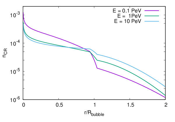
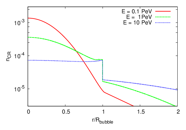
In Fig. 1 we show the normalised CR surface density of a bursting and a continuous source (right) as function of distance in units of the bubble radius for three different energies [10]. Let us discuss first the case of a bursting source shown in the left panel after the time $t=3000$ yr: At low energies, $E\raise 1.29167pt\hbox{$\;<$\kern-7.5pt\raise-4.73611pt\hbox{$\sim\;$}}0.1$ PeV, the Gaussian diffusion front $\propto(2Dt)^{1/2}$ (with $D$ as the diffusion coefficient inside the bubble) has not reached yet the bubble wall. The small fraction of CRs which left already the bubble feels the stronger magnetic field outside, leading to a slower decrease of the CR density at $r>R$. Thus the CR density is described by a quasi-Gaussian density profile with two effective diffusion coefficients inside and outside the bubble¹¹ 1 Andersen [10] discusses fits of various analytical toy models to the CR density inside and outside of the bubble.. In contrast, at the highest energy considered, $E=10$ PeV, CRs propagate inside the bubble close to the ballistic regime, being then “slowed” down by the increased diffusion in the bubble wall. Thus the bubble wall acts as a kind of “semi-permeable membrane” increasing the CR density inside the bubble. After a drop in the CR density, a quasi-Gaussian tail is visible outside the bubble. Finally, for the intermediate energy $E=1$ PeV, CRs diffuse also inside the bubble, and a quasi-Gaussian density profile with two effective diffusion coefficients inside and outside the bubble is visible. The main difference between the bursting and the continuous source shown in the right panel is the absence of a characteristique energy below which CRs have not yet reached the bubble wall. As a result, the production of low-energy energy secondary photons is not suppressed.

We consider next the special case of our local neighbourhood. The Sun is situated inside the Local Superbubble, a irregular formed volume of the interstellar medium with an extremely low density and radius $\sim 100$ pc. Egger & Aschenbach [16] noted the possibility of a collision of the nearby Loop I superbubble with the Local Bubble, forming a wall of neutral and dense material in the interaction zone. In this work, we will use the geometry sketched in their Fig. 5. In particular, we will assume that the Sun is close to the wall, choosing as the smallest distance $d=25$ pc. We assume that the interface between the Local Bubble and Loop I has the density $n=20$/cm³, while the remaining bubble wall of Loop I has the density $n=10$/cm³.

Compared to our calculations of CR propagation in our toy model, Loop I has a radius which is three times larger. Moreover, we are interested in a source as Vela which is $\simeq 11.000$ yr old. From the scaling law $L\propto(2Dt)^{1/2}$ we estimate that we can use the results presented in Fig. 1 as a proxy for the case $t\simeq 11.000$ yr and $R\simeq 100$ pc appropriate for the distance of Vela to the center of Loop I. Alternatively, the CR source may be older and the magnetic field strength in Loop I higher than we assumed.

Note that in a two-dimensional geometry as the Galactic disk, sources inside a ring with distance $\rho$ to the observer contribute as $1/\rho$ to the observed flux. Therefore nearby sources contribute strongly even assuming a uniform source distribution $n_{s}$. More explicitly, one can calculate the flux from 100 sources distributed uniformly in the Galactic disk. In Fig. 2, we show the cumulative flux from sources within the distance $d$ normalised such that the total flux is one as a magneta line. While one expects on average the nearest source at the distance $d\simeq 1.5$ kpc, the distance to Vela is $d=0.3$ kpc, leading to an enhancement of its flux by a factor 25. This enhancement becomes stronger, if one takes into account the known spatial distribution of pulsars and SNRs. For instance, Figure 14 of Neronov & Semikoz [30] shows the location of known pulsars with age $<30.000$yr (see also their Table III). Except for Vela, no other pulsar is known within 1 kpc, and many have distances as large as 3–5 kpc. Using this distribution, one obtains for the cumulative flux within the distance $d$ the green line. We conclude that Vela (or other sources in Loop I which are at an exceptional small distance compared to other known pulsars or young SNRs can dominate the total flux from all Galactic sources. This implies also that the extragalactic flux from normal galaxies gives a negligible contribution.

We use the Monte Carlo generator QGSJET-II [34, 35] to calculate the photon and neutrino secondary fluxes. We assume a mass fraction of 24% of Helium in the target gas and calculate the average intensity of the secondaries as

where $\sigma_{\rm inel}^{pA}$ is the production cross section of secondaries of type $i$ in interactions of protons on nuclei with mass number $A$, $d$ denotes the distance from the Sun to the interaction point $\boldsymbol{x}$, $n_{p}(E,\boldsymbol{x})$ the differential number density of CR protons and $n_{\rm gas}^{A}(\boldsymbol{x})$ the density of protons and Helium in the bubble wall of Loop I, respectively. We use as injection spectrum of CR protons $dN/dE\propto E^{-2.2}\exp(-E/E_{0})$ with $E_{0}=3\times 10^{15}$ eV, normalised such that the total energy emitted in CRs is $E_{\rm CR}=2.5\times 10^{50}$ erg. Then we use the normalised CR surface density shown in Fig. 1 to obtain the relevant CR density inside the bubble wall.

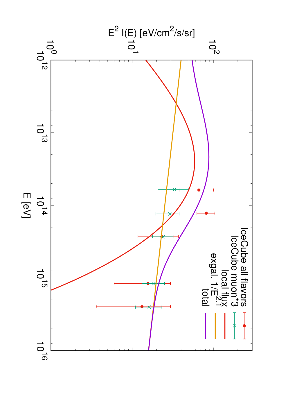
In Fig. 3 we show by a red line the resulting intensity $I(E)$ multiplied by $E^{2}$ of neutrinos on Earth obtained in our model. An extragalactic component with spectral shape $1/E^{2.1}$ as fit to the muon data is shown by an orange line. Finally, the total intensity as sum of the two components is shown by a violet line. While the neutrino intensity of the Galactic component drops below $10^{14}$ eV because CRs with energy lower than $10^{15}$ eV have not reached yet the bubble wall, it is suppressed at high energies because of the assumed cutoff in the CR injection spectrum. The combined neutrino intensity of the Galactic and extragalactic contributions gives a good fit of the experimental data [6]. In most concrete models for extragalactic neutrinos, the predicted intensity is not a pure power law. For instance, the neutrino intensity predicted in Ref. [21] becomes steeper than an $1/E^{2}$ power law below $10^{14}$ eV, leading thus to a more pronounced neutrino bump. Since photon absorption plays for the small distances considered no role, the corresponding photon flux is uniquely determined. An important constraint on our model comes therefore from the limits on the diffuse gamma-ray flux in the 100 TeV–1 PeV energy range [8], which were imposed in particular by the KASCADE experiment from the non-observation of photon-like events at those energies. Note that this limit was reconsidered recently by the KASCADE-Grande collaboration taking into account post-LHC hadronic models.

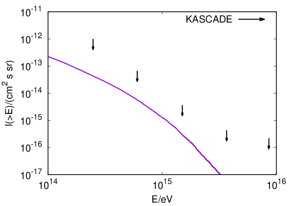
In Fig. 4 we show that the integral photon intensity $I(>E)$ obtained in our model as function of energy $E$ obeys the upper $90\%$ C.L. derived from KASCADE data [11]. Note however that the predicted photon flux is only a factor few below the KASCADE limit, which makes it detectable by future experiments. Additionally, the arrival directions of photon-like events in the KASCADE data could be used already now to constrain a possible flux enhancement towards Loop I.

Finally, let us comment on the deviation expected in our scenario from an isotropic neutrino flux. The sky region in the direction of the Loop 1 superbubble is approximately circular with radius $60^{\circ}$, centered at at the Galactic coordinates $l=329.5^{\circ}$ and $b=17.5^{\circ}$. In the 6 year IceCube data set, 15 out of 28 events (54 %) with $E>100$ TeV are located in this region, while one expect 8.6  events according to the IceCube exposure for an isotropic flux (or 31%). Thus the current dataset shows an excess in this region corresponding to 23% of the total number of events. Dedicated data analyses by the IceCube and the ANTARES collaborations will have the potential to constrain or to favour this scenario in the future.

The explanation of the IceCube data requires in addition to an extragalactic component with a hard spectrum $1/E^{\alpha}$ and $\alpha=2.0-2.2$ a soft Galactic component with the spectral slope $\alpha\simeq 2.5$ [32, 31, 36, 29]. The bounds on the diffuse extragalactic gamma-rays suggest that such a soft component has a Galactic origin. A Galactic neutrino component can be decomposed into two contributions, depending on their angular distribution: Neutrinos from sources in the Galactic plane which are not nearby, and neutrinos from local sources. The first component is strongly limited by the recent bounds on the neutrino contribution from the Galactic plane [5].

In this Letter we studied the possibility that a nearby CR source contributes to the astrophysical neutrino flux. In particular, we studied a model where the CR source is located inside or nearby a superbubble, created by previous supernovae. Both the magnetic field strength and the gas density are enhanced in the wall of a superbubble. As a result, neutrinos are preferentially produce in the wall of the superbubble. If the observer is close to such a superbubble, neutrino events are distributed over a considerable fraction of the sky. We applied then this mechanism to the case of our local neighbourhood in the Galaxy. In particular, we considered the Local and the Loop I superbubbles which are interacting and have an “interaction wall” in between them. As an example for a young nearby CR source may serve the Vela supernova which exploded 11000 years ago. The neutrino flux resulting in this model shown in Fig. 3 can be responsible for a significant part of the IceCube neutrino flux at $\sim{\rm few}\times 100$ TeV and below. Other sources should provide only one half of the flux predicted for Vela, cf. with Fig. 2. A signature of this scenario are the correlation of the arrival direction of Galactic astrophysical neutrinos with the matter distribution in the walls of the Local and the Loop I superbubbles. The contribution to the neutrino signal from the former source would be rather isotropic, and thus resemble the extragalactic component because we are sitting inside this superbubble (but not at its center).

An important constraint on any Galactic neutrino model comes from the limits on high-energy gamma-rays in the 100 TeV–1 PeV energy range. We showed that the predicted photon flux in our model is only a factor few below the KASCADE limits which makes a detection possible for future experiments. Such a detection which would add additional angular information could confirm that both neutrinos and gamma-rays are produced by cosmic ray interactions in the wall between the Local and the Loop I superbubbles. However, the connection to a concrete cosmic ray source model has to be additionally proven. For instance, secondary acceleration on the wall of the Loop I superbubble may be operating as an additional acceleration mechanism [15, 38, 7]. With or without secondary acceleration, the identification of a fraction of IceCube neutrinos as Galactic ones implies the existence of a nearby cosmic ray PeVatron. Vela as a young nearby SNR is a good candidate for this source. In this case, the CR spectrum in the energy region of the knee can be dominated by a single source such as Vela, as suggested e.g. by Erlykin & Wolfendale [17]. Such a scenario complements naturally the “local source” proposal of Kachelrieß et al. [22], Kachelrieß et al. [23] where a 2–3 Myr old source dominates the CR energy spectrum in the 1–100 TeV range.

We conclude that our scenario—if confirmed by future observations—opens up the possibility to study a nearby PeVatron at work through multi-messenger observations with neutrinos, gamma-rays and cosmic rays.

References

- [1] Aartsen, M. G., et al. 2013, Science, 342, 1242856, 1311.5238
- [2] ——. 2014, Phys. Rev. Lett., 113, 101101, 1405.5303
- [3] ——. 2015, Astrophys. J., 809, 98, 1507.03991
- [4] ——. 2016, Astrophys. J., 833, 3, 1607.08006
- [5] ——. 2017a, Astrophys. J., 849, 67, 1707.03416
- [6] ——. 2017b, 1710.01191
- [7] Ackermann, M., et al. 2011, Science, 334, 1103
- [8] Ahlers, M., & Murase, K. 2014, Phys. Rev., D90, 023010, 1309.4077
- [9] Albert, A., et al. 2017, Phys. Rev., D96, 062001, 1705.00497
- [10] Andersen, K. J. 2016, Master’s thesis, NTNU Trondheim, available at http://hdl.handle.net/11250/2456366
- [11] Apel, W. D., et al. 2017, Astrophys. J., 848, 1, 1710.02889
- [12] Berezinsky, V., Gazizov, A., Kachelrieß, M., & Ostapchenko, S. 2011, Phys. Lett., B695, 13, 1003.1496
- [13] Berezinsky, V. S., Gaisser, T. K., Halzen, F., & Stanev, T. 1993, Astropart. Phys., 1, 281
- [14] Breitschwerdt, D., Freyberg, M. J., & Egger, R. 2000, A&A, 361, 303
- [15] Bykov, A. M., & Toptygin, I. N. 2001, Astronomy Letters, 27, 625
- [16] Egger, R. J., & Aschenbach, B. 1995, A&A, 294, L25, astro-ph/9412086
- [17] Erlykin, A. D., & Wolfendale, A. W. 1997, J. Phys., G23, 979
- [18] Evoli, C., Grasso, D., & Maccione, L. 2007, JCAP, 0706, 003, astro-ph/0701856
- [19] Gaisser, T. K., Halzen, F., & Stanev, T. 1995, Phys. Rept., 258, 173, hep-ph/9410384, [Erratum: Phys. Rept.271,355(1996)]
- [20] Giacalone, J., & Jokipii, J. R. 1999, ApJ, 520, 204
- [21] Kachelrieß, M., Kalashev, O., Ostapchenko, S., & Semikoz, D. V. 2017a, Phys. Rev., D96, 083006, 1704.06893
- [22] Kachelrieß, M., Neronov, A., & Semikoz, D. V. 2015, Phys. Rev. Lett., 115, 181103, 1504.06472
- [23] ——. 2017b, Phys. Rev. D97, 063011, 1710.02321
- [24] Kachelrieß, M., & Ostapchenko, S. 2014, Phys. Rev., D90, 083002, 1405.3797
- [25] Krause, M., Charbonnel, C., Decressin, T., Meynet, G., & Prantzos, N. 2013, Astron. Astrophys., 552, A121, 1302.2494
- [26] Loeb, A., & Waxman, E. 2006, JCAP, 0605, 003, astro-ph/0601695
- [27] Mannheim, K. 1995, Astropart. Phys., 3, 295
- [28] Murase, K., Ahlers, M., & Lacki, B. C. 2013, Phys. Rev., D88, 121301, 1306.3417
- [29] Neronov, A., Kachelrieß, M., & Semikoz, D. V. 2018, 1802.09983, to appear in Phys. Rev.
- [30] Neronov, A., & Semikoz, D. V. 2012, Phys. Rev., D85, 083008, 1201.1660
- [31] ——. 2016a, Astropart. Phys., 75, 60, 1509.03522
- [32] ——. 2016b, Phys. Rev., D93, 123002, 1603.06733
- [33] ——. 2016c, Astropart. Phys., 72, 32, 1412.1690
- [34] Ostapchenko, S. 2008, Phys. Rev., D77, 034009, hep-ph/0612175
- [35] ——. 2011, Phys. Rev., D83, 014018, 1010.1869
- [36] Palladino, A., Mascaretti, C., & Vissani, F. 2017, Eur. Phys. J., C77, 684, 1708.02094
- [37] Palladino, A., & Winter, W. 2018, 1801.07277
- [38] Parizot, E., Marcowith, A., van der Swaluw, E., Bykov, A. M., & Tatischeff, V. 2004, Astron. Astrophys., 424, 747, astro-ph/0405531
- [39] Schulreich, M. M., Breitschwerdt, D., Feige, J., & Dettbarn, C. 2017, Astron. Astrophys., 604, A81, 1704.08221
- [40] Stecker, F. W., Done, C., Salamon, M. H., & Sommers, P. 1991, Phys. Rev. Lett., 66, 2697, [Erratum: Phys. Rev. Lett.69,2738(1992)]
- [41] van Marle, A. J., Meliani, Z., & Marcowith, A. 2012, Astron. Astrophys., 541, L8, 1204.2078
- [42] ——. 2015, Astron. Astrophys., 584, A49, 1509.00192
- [43] Waxman, E., & Bahcall, J. N. 1997, Phys. Rev. Lett., 78, 2292, astro-ph/9701231