Core Discovery in Hidden Graphs
Abstract.
Network exploration is an important research direction with many applications. In such a setting, the network is, usually, modeled as a graph , whereas any structural information of interest is extracted by inspecting the way nodes are connected together. In the case where the adjacency matrix or the adjacency list of is available, one can directly apply graph mining algorithms to extract useful knowledge. However, there are cases where this is not possible because the graph is hidden or implicit, meaning that the edges are not recorded explicitly in the form of an adjacency representation. In such a case, the only alternative is to pose a sequence of edge probing queries asking for the existence or not of a particular graph edge. However, checking all possible node pairs is costly (quadratic on the number of nodes). Thus, our objective is to pose as few edge probing queries as possible, since each such query is expected to be costly. In this work, we center our focus on the core decomposition of a hidden graph. In particular, we provide an efficient algorithm to detect the maximal subgraph of of where the induced degree of every node is at least . Performance evaluation results demonstrate that significant performance improvements are achieved in comparison to baseline approaches.
Keywords:
hidden graphs, core decomposition, graph mining1. Introduction
Graphs are ubiquitous in modern applications due to their power in representing arbitrary relationships among entities. Organizing friendship relationships in social networks, modeling the Web, monitoring interactions among proteins are only a few application examples where the graph is a first class object. This significant interest in graphs is the main motivation for the recent development of efficient algorithms for graph management and mining (Cook and Holder, 2006; Aggarwal and Wang, 2010).
A graph or network is composed of a set of vertices and a set of edges denoted as . In its simplest form, is undirected (no direction is assigned to the edges) and unweighted (the weight of each edge is assumed to be 1). Vertices represent entities whereas edges represent specific types of relationships between vertices. Due to their rich structural content, graphs provide significant opportunities for many important data mining tasks such as clustering, classification, community detection, frequent pattern mining, link prediction, centrality analysis and many more.
Conventional graphs are characterized by the fact that both the set of vertices and the set of edges are known in advance, and are organized in such a way to enable efficient execution of basic tasks. Usually, the adjacency lists representation is being used, which is a good compromise between space requirements and computational efficiency. However, a concept that recently has started to gain significant interest is that of hidden graphs. In contrast to conventional graphs, a hidden graph is defined as , where is the set of vertices and is a function which takes as an input two vertex identifiers and returns true or false if the edge exists or not respectively. Therefore, in a hidden graph the edge set is not given explicitly and it is inferred by using the function .
The brute-force approach for executing graph-oriented algorithmic techniques on hidden graphs comprises the following phases:
- )
in the first phase, all possible edge probes are executed in order to reveal the structure of the hidden graph completely, and
- )
in the second phase, the algorithm of interest is applied to the exposed graph.
It is evident, that such an approach is not an option, since the function associated with edge probing queries may be extremely costly to evaluate and it may require the invocation of computationally intensive algorithms. The following cases are a few examples of hidden graph usage in real-world applications:
(a) 1-core

(b) 2-core

(c) 3-core (max core)
- •
A hidden graph may be defined on a document collection, where returns 1 if the similarity between two documents is higher than a user-defined threshold and 0 otherwise. Taking into account that there are many diverse similarity measures that can be used, it is more flexible to represent the document collection as a hidden graph , using to determine the level of similarity between documents.
- •
Assume that the vertices of the graph are proteins, forming a protein-protein interaction network (PPI). An edge between two proteins and denotes that these proteins interact. Edge probing in this case corresponds to performing a lab experiment in order to validate if these two proteins interact or not. In this case, the computation of the function is extremely costly.
- •
Relational databases may be seen as hidden graphs as well. In this scenario, the vertices of the hidden graph may be database records or entities, whereas the edges may correspond to arbitrary associations between these entities (corresponding to a -join). For example, in an product-supplier database, vertices may represent suppliers and an edge between two suppliers may denote the fact that they supply at least a common product with specific properties. In this case, the function involves the execution of a possibly complex SQL join query.
- •
As another example, consider the set of vertices defined by user profiles in a social network. A significant operation in such a network is the discovery of meaningful communities. However, there is a plethora of methods to quantify the strength or similarity among users, ranging from simple metrics such as number of common interests to more complex ones like the similarities in their posts, or their mutual contribution in answering questions (like in the case of the Stack Overflow network). In these cases, taking into account that user similarity can be expressed in many diverse ways, the hidden graph concept is very attractive for ad-hoc community detection.
Hidden graphs constitute an interesting tool and an promising alternative to conventional graphs, since there is no need to represent the edges explicitly. This enables the analysis of different graph types that are implicitly produced by changing the function . Note that the total number of possible graphs that can be produced for the same set of vertices equals , where is the number of vertices. It is evident, that the materialization of all possible graphs is not an option, especially when is large. Therefore, hidden graphs is a tempting alternative to model relationships among a set of entities. On the other hand, there are significant challenges posed, since the existence of an edge must be verified by evaluating the function , which is costly in general.
A significant graph mining task, which is highly related to community detection and dense subgraph discovery, is the core decomposition of a graph. The output of the core decomposition process is a set of nested induced subgraphs (known as cores) of the original graph that are characterized by specific constraints on the degree of the vertices. In particular, the 1-core of is the maximal induced subgraph , where the degree of every vertex in is at least 1. The 2-core of is the maximal induced subgraph , where all vertices have degree at least 2. In general, the -core of is the maximal induced subgraph where the degree of every vertex in is at least . In addition, for any two core subgraphs and , if then .
Based on the fact that the cores of a graph are nested, the core number of a node is defined as the maximum value of such that participates in the -core. The maximum core value that can exist in the graph is also known as the graph degeneracy (Farach-Colton and Tsai, 2014). Formally, the degeneracy of a graph is defined as the maximum for which contains a non-empty -core subgraph.
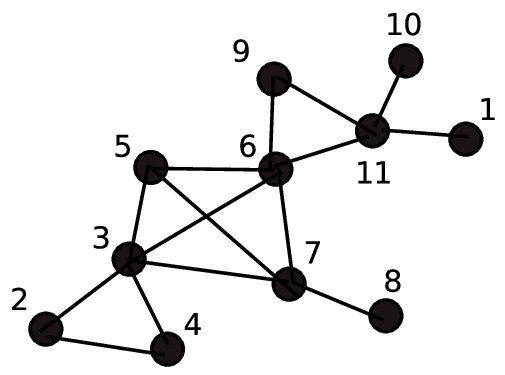
A core decomposition example is illustrated in Figure 1. Black-colored nodes participate in the corresponding core. Therefore, the graph in Figure 1(a) corresponds to the 1-core of , since the degree of all nodes is at least one and there is no supergraph with this property. Similarly, Figures 1(b) and 1(c) show the 2-core and the 3-core of respectively. Note that the induced subgraph representing the -core contains nodes with degree at least and there is no larger subgraph with this property. Note also, that the maximum core of the graph is the 3-core, since beyond that point it is not possible to form an induced subgraph such that the degree of the nodes is at least 4. If one of the nodes participating in the maximum core is removed, the graph collapses. Thus, based on the definition of the graph degeneracy, in this case .
Motivation and Contributions.
The core decomposition of graphs has many important applications in diverse fields (Malliaros et al., 2016). It has been used as an algorithm for community detection and dense subgraph discovery (Fortunato, 2010), as a visualization technique for large networks (Alvarez-Hamelin et al., 2006), as a technique to improve effectiveness in information retrieval tasks (Rousseau and
Vazirgiannis, 2015), as a method to quantify the importance of nodes in the network in detecting influential spreaders (Rossi
et al., 2015), and as a tool to analyze protein-protein interaction networks (Altaf-Ul-Amine
et al., 2003), just to name a few.
In this work, we apply the concept of core decomposition in a hidden graph.
The fact that the graph is hidden, poses significant difficulties in the discovery of the -core. First of all, since the edges are not known in advance, edge probing queries must be executed to reveal the graph structure. In addition, specialized bookkeeping is required in order not to probe an edge multiple times. Formally, the problem we attack has as follows:
PROBLEM DEFINITION. Given a hidden graph , where is the set of nodes and a probing function, and an integer , discover a -core of if such a core does exist, by using as few edge probing queries as possible.
To the best of the authors’ knowledge, this is the first work studying the problem of -core computation in a hidden graph. In particular, we present the first algorithm to compute the -core of a hidden graph, if such a core exists. Our solution is based on the following methodology:
- (1)
Firstly, we generalize the SOE (switch-on-empty) algorithm proposed in (Tao et al., 2010) in order to be able to determine nodes with high degrees in any graph, since the initial SOE algorithm supports only bipartite graphs and determines the largest degrees focusing only in one of the two bipartitions. In addition, the generalized algorithm can also be applied in directed graphs with minor modifications.
- (2)
Secondly, we enhance the generalized algorithm (GSOE) with additional data structures in order to provide efficient bookkeeping during edge probing queries.
- (3)
Finally, we provide the HiddenCore algorithm which takes as input an integer number and either returns the -core of or false if the -core does not exist. Although HiddenCore is based on GSOE, it uses different termination conditions and performs additional bookkeeping to deliver the correct result.
Performance evaluation results have shown that significant performance improvement is achieved in comparison to the baseline approach which performs all possible edge probing queries in order to reveal the structure of the graph completely.
Roadmap. The rest of the paper is organized as follows. Section 2 presents related work in the area, covering the topics of core decomposition and hidden graphs. Section 3 contains some background material useful for the upcoming sections. The proposed methodology is given in detail in Section 4. Performance evaluation results are offered in Section 5 and finally, Section 6 concludes the work and discusses briefly interesting topics for future research in the area.
2. Related Work
Hidden graphs have attracted a significant attention recently, since they allow the execution of graph processing tasks, without the need to now the complete graph structure. This concept was originally introduced in (Grebinski and Kucherov, 1998), where edge probing queries were used to test if there is an edge between two nodes.
One research direction which uses the concept of edge probes is graph property testing (Goldreich et al., 1998), where one is interested to know if a graph has a specific property, e.g., if the graph is bipartite, if it contains a clique, if it is connected, and many more. However, in order to test if the graph satisfies a property or not, the number of edge probing queries must be minimized, leading to sublinear complexity with respect to the number of probes. Moreover, these algorithms are usually probabilistic in nature and provide some kind of probabilistic guarantees for their answer, by avoiding the execution of a quadratic number of probes.
Another research direction related to hidden graphs, focuses on learning a graph or a subgraph by using edge probing queries using pairs or sets of nodes (group testing) (Alon and Asodi, 2005). A similar topic is the reconstruction of subgraphs that satisfy certain structural properties (Bouvel et al., 2005).
One of the problems related to reconstruction, is the discovery of the nodes with the highest degree. In (Tao et al., 2010), the SOE (Switch-on-Empty) algorithm is proposed to solve this problem in a bipartite graph. It has been shown that SOE is significantly more efficient than the baseline approach which simply reveals the graph structure by executing all possible edge probing queries. The same problem has been also studied in (Yiu et al., 2013) using combinatorial group testing, which allows edge probing among a specific set of nodes instead of just one pair of nodes.
The core decomposition is a widely used graph mining task with a significant number of applications in diverse fields (Malliaros et al., 2016). The concept was first introduced in (Seidman, 1983) and later on it was adopted as an efficient graph analysis and visualization tool (Alvarez-Hamelin et al., 2005; Zhang and Parthasarathy, 2012). The baseline algorithm to compute the core decomposition requires operations and it is based on a minheap data structures with the decrease key operation enabled ( is the number of edges and the number of node). The algorithm gradually removes the node with the smallest degree, updating node degrees as necessary. A more efficient algorithm with linear complexity was proposed in (Batagelj and Zaversnik, 2003). The algorithm uses bucket sorting and multiple arrays of size to achieve linearity.
There is a plethora of algorithms for the computation of the core decomposition under different settings and computational models. Some of these efforts are: disk-based computation (Cheng et al., 2011), incremental core decomposition (Saríyüce et al., 2013), distributed core decomposition computation (Montresor et al., 2013; Pechlivanidou et al., 2014), local core number computation (O’Brien and Sullivan, 2014), core decomposition of uncertain graphs (Bonchi et al., 2014).
The main characteristic of the aforementioned core decomposition algorithms is that in order to operate, the set of edges must be known in advance. In the sequel, we present our solution for detecting cores in hidden graphs which is based on edge probing queries and it does not requires knowledge of the complete set of edges.
3. Fundamental Concepts
In this section, we discuss some fundamental concepts necessary for the the upcoming material. In particular, we will present briefly the use of the Switch-On-Empty algorithm proposed in (Tao et al., 2010) and also we will discuss the linear core decomposition algorithm reported in (Batagelj and Zaversnik, 2003).
3.1. Preliminaries
| Symbol | Interpretation |
| a hidden graph | |
| set of vertices of | |
| number of vertices of () | |
| vertices of | |
| set of neighbors of vertex | |
| degree of vertex | |
| (unknown) set of edges | |
| (unknown) number of edges () | |
| , | source and destination vertices |
| true if the edge exists, false otherwise | |
| number of highest degree vertices requested | |
| defines the -core of | |
| number of known existing neighbors of | |
| number of known non-existing neighbors of | |
| total number of edge probing queries issued |
The input hidden graph is denoted as , and contains vertices and edges. The number of neighbors of is known as the degree of , . Note that some quantities are not known in advance. For example, the total number of edges , vertex degrees, the diameter, and any value related to the graph edges is unknown. Table 1 summarizes the most frequently used symbols.
Initially, the number of neighbors of each vertex is unknown. As edge probing queries are executed, the graph structure gradually reveals. When an edge probing query between vertices and is executed (i.e., the function is invoked), either the edge exists or not. Two counters are associated with each vertex : the counter counts the number of edges that are solid, i.e., they exist and the counter counts the number of empty, i.e., non-existing edges incident to . Therefore, if exists, then the counters and are incremented. Otherwise the counters and are incremented. The sum measures the number of edge probing queries executed where is one endpoint.
3.2. The Switch-On-Empty Algorithm (SOE)
Before diving into the details of the GSOE algorithm, the original SOE algorithm, proposed in (Tao et al., 2010), is described briefly. In SOE, the input is a bipartite graph, with bipartitions and . The output of SOE is composed of the vertices from or with the highest degree. Without loss of generality, assume that we are focusing on vertices in . Edge probing queries are executed as follows:
- •
SOE starts from a vertex , selects a vertex and executes . If the edge is solid, it continues to perform probes between and another vertex .
- •
Upon a failure, i.e., when the probe returns an empty result, the algorithm applies the same for another vertex . Vertices for which all the probes have been applied, do not participate in future edge probes.
- •
A round is complete when all vertices of have been considered. After each round, some vertices can be safely included in the result set and they are removed from . When a vertex must be considered again, we continue the execution of probes remembering the location of the last failure.
- •
SOE keeps on performing rounds until the upper bound of vertex degrees in is less than the current -th highest degree determined so far. In that case, contains the required answer and the algorithm terminates.
The basic idea behind SOE, is that as long as probes related to a vertex are successful, we must continue probing using that vertex since there are good chances that this is a high-degree vertex. It has been proven in (Tao et al., 2010), that SOE is instance optimal, which means that on any hidden bipartite graph given as an input, the algorithm is as efficient as the optimal solution, up to a constant factor. It has been shown, that this constant is at most two for any value of the parameter (number of vertices with the highest degree).

In the sequel, we provide a simple example to demonstrate the way SOE works to discover the top- vertices with the highest degree. Let denote a hidden bipartite graph, containing vertices and edges as shown in Figure 2. We assume that in our case , i.e., we need to detect the vertex with the highest degree. Without loss of generality we focus on the left bipartition (vertex set ) which contains the vertices , and .
If we apply the brute-force algorithm in this graph, we need to perform all edge probes first, and then simply select the vertex with the highest degree among the subset . In contrast, SOE will perform the following sequence of probes: , , , , , , , . At this stage, SOE knows that vertex will be part of the answer since the degree of can be computed exactly, since all probes related to vertex have been executed. The next probe will be and know SOE can eliminate vertex since its degree cannot be larger than 3 which is the degree of . The next probe is , and now SOE terminates since vertex cannot make it to the answer since . The total number of probes performed by SOE is 10, whereas the brute-force algorithm requires 12.
3.3. Cores in Conventional Graphs
The core decomposition of a conventional graph can be computed in linear time, as it is discussed thoroughly in (Batagelj and Zaversnik, 2003). The pseudocode is given in Algorithm 1 (CoreDecomposition). To achieve the linear time complexity, comparison-based sorting is avoided and instead binsort is applied for better performance, since the degree of every vertex lies in the interval (isolated vertices are not of interest), where is the number of vertices.
Each time, the vertex with the smallest degree is selected and removed from the graph. The selection of the next vertex to remove, is performed in . After vertex removal, the degrees of neighboring vertices are adjusted properly and for each neighbor a reordering is performed, again in time, due to the usage of the bins. Each bin contains vertices with the same degree. Thus, there are at most bins. Since each edge is processed exactly once, the overall time complexity of the decomposition process is for a graph containing vertices and edges.
The linear complexity combined with the usefulness of the decomposition process results in a very efficient process. However, in our case this technique can be applied only when the set of edges is known to the algorithm. In the next section, we present our proposal towards detecting -cores in a general hidden graph.
4. Proposed Methodology
In this section, we present our methodology in detail. Firstly, we focus on the generalization of the SOE algorithm. The Generalized Switch-On-Empty Algorithm (GSOE) is able to find the top- degree vertices in an undirected hidden graph, whereas SOE can be applied on bipartite graphs only. Secondly, we present the algorithmic techniques to enable the discovery of vertices belonging to the -core of the graph, if the -core does exist.
4.1. Bookkeeping
Since SOE focuses only on one of the two bipartitions of the input graph, the bookkeeping process is very simple, because it just needs to remember the last failure of every vertex. However, in a general graph , this cannot be applied, because edge probes may affect the neighborhood list of other vertices. The aim of GSOE is to discover the vertices with the highest degree among all graph vertices, by performing as few edge probing queries as possible and by avoiding probing the same link twice. Each edge probing query is performed from a source vertex towards a destination vertex , by invoking the function . Similarly to SOE, if the probe indicates that there is a connecting edge between and , then this edge is considered as solid otherwise it is marked as empty. Based on the probing result, the algorithm either continues with the same source vertex and a different destination vertex or changes the source vertex as well and selects the next available one.
For the proper selection of source and destination vertices, GSOE stores probing results at vertex-level data structures. As the algorithm evolves, these data structures store the necessary information required for the next selection of source and destination vertices. The result of GSOE is a set containing the vertices with the highest degrees, sorted in non-increasing order. To provide the final result, GSOE maintains the following information for every vertex :
- •
the counter , monitoring the total number of solid edges incident to ,
- •
the set of solid edges, , detected so far for vertex (),
- •
the counter , counting the total number of empty edges incident to ,
- •
the variable is decreased by one whenever participates in an edge probe for which the edge does not exist,
- •
an auxiliary data structure (probe monitoring structure) to be able to detect the next available vertex to act as destination, in order to perform the next edge probing query.
For vertex , the structure performs the necessary bookkeeping regarding the probes performed so far related to . Whenever participates in a probe either as source or destination vertex, is updated accordingly. For the rest of the discussion, we will assume that vertex identifiers take values in the interval , where is the total number of vertices of the hidden graph. Let denote the set of empty edges detected for . Note that, we use this set for the convenience of the presentation, since it is not being used by the algorithm.
First, we focus on the selection of a destination vertex, assuming that the source vertex is known. Later, we will also discuss thoroughly how source vertices are selected. Let be the selected source vertex. We are interested in determining a vertex in order to issue the probing query .
The next destination vertex must satisfy the following property: , i.e., must not have been considered previously. The straight-forward solution to detect , is to consider the union and find the first available vertex identifier. This solution has a time complexity of , because both sets and must be scanned once. Taking into account that can be as large as , we are interested in a more efficient design.
Assume that is part of a hidden graph with vertices. For the purpose of the example, let . Assume further, that at a specific instance the status of the probes is and , which means that and . Since , there are still six available vertices to be selected as destinations. Thus, the set of solid and empty edges define a set of available intervals containing vertex identifiers that can be selected as destinations. Based on our example, the set of available intervals has as follows: , , }. Since intervals are pair-wise disjoint and they never overlap, they can be organized in a balanced binary search tree data structure, where the key corresponds to the left (right) endpoint regarding the left (right) subtrees.

(a) selected: 2

(b) selected: 5

(c) selected: 8

(d) selected: 7

(e) selected: 3

(f) selected: 4
An example is illustrated in Figure 3, showing a sequence of destination selections. Initially, the set of available intervals contains only the interval , whereas and . Let be the first vertex selected as destination and that the probe returns a solid result. This means that and . In fact, for the maintenance of the BST, it does not matter of we have solid or empty edges. All that matters is the vertex being selected as a destination. In this example, the selection order of destinations is arbitrary and the selected vertices are: 2, 5, 8, 7, 3 and 4. In Figure 3, we observe the evolution of the BST as destination vertices are being deleted gradually from the set of available intervals.
Lemma 4.1.
Given a source vertex , the selection of the destination vertex requires time, whereas updating the information of the available destinations requires time.
Proof.
Since each node of the BST contains an interval of available destinations, it suffices to visit the root and select a destination from the corresponding interval of the root node. Evidently, this operation takes constant time. We distinguish between two cases: ) the interval is of the form where strictly and ) the interval is of the form . In the first case, we select as destination either or in order to avoid any structural operations on the BST. Thus, the length of the interval is reduced by one. In the second case, the interval is deleted from the BST. The number of elements in the BST is at most , which means that deletions require time in the worst case. ∎
After updating for the destination vertex , the edge probing query is issued. If , is inserted into and also, is inserted into . In addition, the must be updated as well, which means that the BST associated with vertex must exclude vertex from the available destinations. To facilitate this operation, a lookup in the BST is performed for the key , in order to detect the interval containing . Note that, since intervals are disjoint, is contained in one and only one interval, which can be detected in logarithmic time .
We distinguish among three different cases: ) is included in the interval or and in this case the interval is simply shrunk from the right or the left endpoint respectively. ) is included in the interval , and a single deletion of the vertex is required. ) is included in the interval and and . In this case, the interval is split to two intervals and . The original interval is deleted from the BST whereas the two new subintervals are inserted in the BST. In any case, the cost is
Theorem 4.2.
Given a source vertex , the selection of the destination vertex and the updates of the structures and take time , where is the number of graph vertices.
Proof.
The result follows from Lemma 4.1 and from the fact that the number of intervals that can be hosted by each BST is at most . ∎
So far, we have focused on the selection of a destination vertex, assuming that the source vertex is already known. Next, we elaborate on the selection of the source vertex to participate in the next edge probing query.
4.2. Detecting High-Degree Vertices
Let denote the result set containing at least vertices with the highest degrees. Note that, in case of ties (i.e., if many vertices have the same degree as the -th), these vertices will be also included in . Let be the current source vertex. As long as the probing queries return solid edges, the source vertex remains the same and the structures , , and are updated accordingly, as described in the previous section.
If , i.e., the edge does not exist, the source vertex should change and another vertex is selected as source. In GSOE, the following rules are applied:
- Rule 1
When the probing comes out solid, the values and are increased by one.
- Rule 2
When the probing comes out empty, the values , , and are decreased by one.
- Rule 3
A vertex can be pushed to the result set if GSOE found its actual degree and .
- Rule 4
When a vertex has it cannot be selected as a source vertex. It can only be selected as a destination vertex. A vertex can be selected as a source vertex only if and it does not fulfill Rule 3.
GSOE terminates when no more vertices can be added in the result set . This means that the maximum potential degree for a vertex is strictly less than the -th best degree contained in .
The sequence of probing queries is performed in rounds. If is the first vertex to be checked as a potential sourse, a round is complete when is checked again as a potential source vertex. If it fulfills the necessary requirements stated by Rule 4 above, then it will be selected as the next source.
Lemma 4.3.
For every vertex , it holds that equals the number of rounds spent while .
Proof.
From the definition of , we conclude that when is increased by one then is decreased by one. This means that is decreased times. According to Rule 3, GSOE pushes a vertex to only if this vertex has zero state. Recall that a negative value is increased by one at the end of each round. Thus, for a vertex that is pushed in it holds that the value equals the number or rounds performed with . In case after GSOE terminates, then equals the number of rounds needed for to be included in . ∎
Lemma 4.4.
Two or more vertices are pushed in during the same round if and only if they have the same degree.
Proof.
We provide the proof for two vertices and since the generalization is obtained easily. Assume that and are pushed to during the same round. This means that GSOE had spent the same number of rounds until it pushes them to . Based on 4.3 we conclude that: . Since and are both contained in it holds that: = and =, which means that = and thus, . ∎
The usefulness of the previous lemma lies in the fact that all vertices having the same degree as the -th best vertex, will enter the result set during the same round, and therefore the termination condition of the algorithm is based only on the number of elements contained in set . Consequently, the condition is sufficient to terminate and it guarantees that the result set is correct.
The outline of GSOE is given in Algorithm 3. New vertices are inserted into the result set at Lines 5, 15 and 17. The termination condition is checked at Lines 19 and if it is satisfied the algorithm returns the set containing the high-degree vertices, otherwise it continues with the next source vertex. After each probe, the bookkeeping structures are updated accordingly at Line 10 where the Update function (shown in Algorithm 2) is invoked.
4.3. Core Discovery
In the previous section, we discussed a solution for solving the problem of detecting the vertices with the highest degrees in a hidden graph , using the Generalized Switch-On-Empty algorithm. In this section, we dive into the problem of discovering the -core of , if such a core does exist. We remind that the -core of is the maximal induced subgraph where for each vertex , . To attack the problem, we propose the HiddenCore algorithm, which extends GSOE by using different criteria for selecting source and destination vertices and different termination conditions to guarantee efficiency and correctness.
In order for a vertex to belong to the -core, . After an empty probe, HiddenCore estimates the maximum degree value that source and destination vertices could reach. For this purpose, HiddenCore introduces a new vertex-level parameter called potential degree. In a hidden graph with vertices, it holds that . If the potential degree of a vertex becomes less than , then HiddenCore blacklists this vertex. This practically means that probings from or towards this vertex is useless and thus, this vertex will be ignored for the rest of the algorithm execution. The value of is updated every time there is en empty probe related to vertex , i.e., participates either as source or destination vertex.
Based on the definition of the -core, in order for a graph to have a -core there must be at least vertices with degree greater than or equal to . Once HiddenCore realizes that it is impossible to satisfy this property, it terminates with a false result, since the -core does not exist in . To enable this process, we introduce the concept of the number of potential core vertices, symbolized as . Initially, , since all vertices are candidates to be included in the -core. Gradually, as more empty probes are introduced, whenever for a vertex , , the value of is decreased by one. Consequently, if during the course of the algorithm the value of becomes less than , the algorithm terminates with a false result, since it is impossible to detect the -core in .
The aforementioned termination condition cannot restrict the number of probes issued as long as . This means that HiddenCore will terminate when all possible probes are executed. To handle this case, we introduce the maximum potential degree variable which is the maximum value of , for all vertices of not yet in , and it is formally defined as follows:
The value of is checked at the end of every round. If , then we know that no additional vertices will ever satisfy the conditions to enter the result. Consequently, HiddenCore can proceed by executing the CoreDedomposition algorithm. The first condition is applied after every probe, whereas the second one is applied after each round. The combination of the two aforementioned termination conditions leads to a significant reduction in the number of probes.
Note that, HiddenCore is able to detect vertices that cannot make it to the final result by examining their potential to raise the number of solid edges to . However, a more aggressive termination condition can be applied that takes into account the potential of finding at least vertices, based on the number of probes still available. More specifically, let denote the set of vertices with the highest number of solid edges detected. These vertices can be effectively organized using a minheap data structure, which is updated after each probe. The vertices in define a lower bound on the number of probes required in order for the CoreDecomposition algorithm to be applied. Any vertex , requires additional probes to have chances to increase its degree above . Therefore, the total requirements with respect to the minimum number of additional probes needed is given by the following formula (note: stands for the number of required probes):
This number must be less than or equal to the number of available probes (), that we can still issue. Evidently, it holds that:
Based on the previous discussion, HiddenCore must terminate its execution whenever . The value of can be monitored efficiently by updating the contents of the set , and this requires logarithmic time with respect to the size of , which is .
During the course of the algorithm, a subgraph is constructed, which accommodates all graph vertices where . Also, satisfies the constraint . It is important to note that the subgraph does not contain any hidden edges, and therefore no additional probes are required to reveal its structure completely. The last phase of HiddenCore involves the execution of the CoreDecomposition algorithm (Algorithm 1), in order to decide if the -core exists or not. This is necessary, since the degree constraint of vertices in involves the whole graph and not the subgraph induced by . The following lemma guarantees the correctness of the result returned by HiddenCore.
Lemma 4.5.
The -core of exists, if at least vertices in have a core number greater or equal to .
Proof.
In case all vertices in have a core number exactly , we are done since this is the definition of the -core. However, it may be the case that CoreDecomposition decides that all core numbers are strictly larger than . This means that higher-order cores are available, and due to the fact that cores are hierarchically nested, also lower-order cores must exist as well, and therefore no vertex will be missed. ∎
A pleasant side effect of the above result is that if the -core does exist, due to the execution of the CoreDecomposition algorithm, higher order cores are also directly available. Therefore, HiddenCore is able to compute the complete core decomposition of the hidden graph for the subset of vertices that are contained in the -core of .
Also, we note that HiddenCore can be used for core discovery in hidden directed graphs as well, where edge directionality is important. Evidently, the definition of the result and the termination conditions should be updated accordingly to reflect the fact that each vertex contains a set of outgoing edges, and a set of incoming edges. The concept of core decomposition in directed graphs has been covered in (Giatsidis et al., 2011) and it has many important applications, since a significant part of real-world graphs are directed.
The pseudocode of the proposed technique is summarized in Algorithms 4 and 5. Early termination is possible at Lines 21-24, when HiddenCoreCheck fails to satisfy the requirements. If the execution reaches Line 7, the CoreDecomposition algorithm is invoked to discover the -core. At this stage, again we have two options: ) either the -core exists and the algorithm returns the corresponding subgraph, or ) the -core does not exist, in which case the algorithm returns the empty set.
To demonstrate the way HiddenCore operates, in the sequel we provide a running example based on the small graph shown in Figure 4. We provide two different cases with respect to the result: ) the requested -core does not exist (negative answer) and ) the requested -core does exist (positive answer). Tables 2 to 5 depict the actions taken and the status of each probe applied, depending on the outcome (solid or empty).

Firstly, let us assume that the user is interested in the 4-core of the hidden graph , and thus, . Table 2 shows the actions taken. In particular, after the fist empty probe , the algorithm terminates because there are at least two vertices (1 and 3) with degree less than , and therefore, the -core does not exist in . Out of the 10 possible probes, only two of them were executed which is translated to 80% gain with respect to the number of probes.
Secondly, we check the progress of HiddenCore for . Tables 3 and 5 depict the actions taken for the 1st and 2nd round respectively. Note that, one round is not adequate for the algorithm to terminate, since the termination condition is not satisfied. Moreover, Table 4 shows the values of the most important variables. In this case, out of the 10 possible probes, 9 of them are executed by HiddenCore, resulting in a 10% gain.
| Probe | Actions/Notes |
| - ++ and ++ | |
| - ++ and ++ - and which is less than and so they are eliminated. - is less than - HiddenCore terminates and returns false |
| Probe | Actions/Notes |
| - ++ and ++ | |
| - ++ and ++ - , - and - continue | |
| - ++ and ++ | |
| - ++ and ++ | |
| - ++ and ++ - vertex 2 is inserted into | |
| - vertex 3 cannot become a source because . - ++ and ++ - and - and () - vertex 1 is eliminated - - continue | |
| - vertex 1 cannot be a destination (pruned) - vertex 2 cannot be a destination because the probe has been used - vertex 3 is the next destination - ++ and ++ | |
| - ++ and ++ - no available probes for vertex 5 - vertex 5 is inserted to - end of Round 1 |
| Vertex | status | ||||
| 1 | 1 | 2 | -2 | 2 | eliminated |
| 2 | 4 | 0 | 0 | 4 | in |
| 3 | 2 | 1 | -1 | 3 | in |
| 4 | 2 | 1 | -1 | 3 | in |
| 5 | 3 | 0 | 0 | 3 | in |
| Probe | Actions/Notes |
| - ++ and ++ - no more probes for vertices 3 and 4 - both are inserted to with degree 3 - all vertices with degree - have been detected we - invoke CoreDecomposition - the 3-core does exist - HiddenCore returns a positive result |
4.4. Runtime Cost and Complexity
We conclude this part of the paper by discussing about the overall cost of the HiddenCore algorithm. Note that, the runtime cost is mainly defined by the number of edge probing queries issued. Assuming that the cost of each probing query, i.e., the computation of the function , is significant, reducing the number of probes is essential.

(a) ego-Facebook

(b) ca-HepPh

(c) soc-Gplus

(d) email-Enron

(e) power-law5K
The second factor that has a direct impact on the performance of the algorithm is the number of primitive operations performed. This may refer to the number of comparisons performed, or the number of searches in lookup tables, and many more. In general, the cost of a probe execution is several orders of magnitude more expensive than a primitive operation and one may think that the total runtime cost is defined by the number of probes. However, this is true because if the number of primitive operations increases significantly, the computational cost may increase significantly as well. For example, an algorithm that requires 1000 probes and primitive operations may be more efficient than another algorithm which needs 10 probes and primitive operations. Therefore, it is essential to minimize the number of probes, as well as the number of primitive operations per probe.
Let denote the total number of probes issued by the algorithm. Based on the previous discussion, each probe triggers a sequence of primitive operations that are at most , resulting in a total complexity of devoted for updating the bookkeeping data structures. Moreover, for each probe issued there is additional cost to update the minheap data structure that accommodates the vertices with the highest number of solid edges. However, this cost does not change the complexity since always .
To that, we need to also add the cost for running the CoreDecomposition algorithm which is in . It is very interesting to provide lower bounds with respect to the number of probes that are required for the discovery of the -core, as a function of the number of vertices and other structural properties.
5. Performance Evaluation
This section contains performance evaluation results, demonstrating the runtime costs of the GSOE algorithm both for detecting high degree vertices and for the discovery of the -core of a hidden graph. All techniques are implemented in the C++ programming language. For the experiments, we have used real-world as well as synthetic graphs following a power-law degree distribution. The data sets used are summarized in Table 6.
| Graph | #vertices ( | #edges () |
| ego-Facebook | 4,039 | 88,234 |
| ca-HepPh | 12,008 | 118,521 |
| soc-Gplus | 23,600 | 39,200 |
| email-Enron | 36,692 | 183,831 |
| power-law1K | 1,000 | 50,000 |
| power-law2K | 2,000 | 100,000 |
| power-law3K | 3,000 | 150,000 |
| power-law5K | 5,000 | 250,000 |
The real-world graphs have been downloaded from the SNAP repository at Stanford (http://snap.stanford.edu) and the Network repository (http://networkrepository.com). For the synthetic graphs we have used the GenGraph tool, which implements the graph generation algorithm described in (Vigen and Latapy, 2005). In particular, GenGraph generates a set of integers in the interval obeying a power-law distribution with exponent . These integers are used as the degree sequence and they define the degrees of the vertices of the synthetic graph that is produced.
| ego-Facebook | ca-HepPh | soc-Gplus | email-Enron | power-law5K | |
| 10 | 0.4% | ||||
| 25 | 0.2% | ||||
| 40 | 0.2% | ||||
| 100 | 2.4% | 0.8% | |||
| 200 | 7% | ||||
| 500 | 21.2% | 8% | 4% | 2.5% | 9.9% |
| 1,000 | 42.1% | 8.2% | 5% | 19% | |
| 2,000 | 74% | 30.3% | |||
| 5,000 | 66% | 38% | 25% | ||
| 10,000 | 68% | 47% |
Figure 5 depicts the performance of the HiddenCore algorithm for all available data sets. In particular, we monitor the total number of probes vs. the parameter , which defines the order of the requested core. We observe that as increases, the total number of probes decreases significantly. By using higher values, we are requesting cores that contain more vertices (at least ) with higher degree (at least ). Therefore, the early termination conditions of the HiddenCore algorithm have more chances to be fulfilled resulting in better performance than the brute force algorithm which requires all probes to be executed first.

(a)

(b)
On the other hand, as we reduce , more probes are required in order to rank the appropriate vertices. This is due to the fact that more vertices survive the constraints and therefore, more probes will be required to completely determine their degree, before the invocation of CoreDecomposition. This leads to an increase in the total number of probes.
Table 7 shows the percentage gain on the total number of probes issued, for different values of and different graphs. As expected, for small values a significant number of probes is performed. As increases, more probes are saved.
Finally, in Figure 6, we depict the number of probes issued vs. the size of the synthetic power-law graph, for two different values of (50 and 100). Note that, as the number of vertices increases, the number of edges increases too, as shown in Table 6. We observe that for the same value of , the number of probes also increases rapidly, showing a quadratic rate of growth. This behavior is explained by the fact that the maximum number of probes also grows in a quadratic rate, since for vertices the maximum number of probes equals .
By observing the experimental results we conclude that probe savings is extremely hard for small values of , provided that we need a 100% accurate answer regarding the existence of the -core. We believe that there is still room for improvements towards reducing the number of probes further. Moreover, it turns out that detecting the largest value of for which the -core exists is an even more challenging problem.
6. Conclusions and Future Work
Hidden graphs are extremely flexible structures since they can represent associations between entities without storing the edges explicitly. This way, many different relationship types can be described, since the only change is the function that should be invoked to reveal the existence of an edge .
In such a setting, existing graph algorithms cannot be applied directly, since the set of neighbors for each node is not known in advance. Since edge probing queries may be extremely expensive to execute (i.e., may involve running complex algorithmic techniques), the aim is to minimize their number as much as possible, to guarantee efficient execution.
In this work, we have studied the problem of core detection in hidden graphs: given a hidden graph and an integer , detect the -core of , or return false if such a core does not exist. In general, the core decomposition problem in conventional graphs (i.e., graphs with a known set of edges) can be solved in linear time , where is the number of nodes and is the number of edges. However, to be able to apply the linear algorithm, the set of edges must be known in advance, meaning that probes must be executed first, which is extremely costly.
We have shown that by using a generalization of the Switch-On-Empty (SOE) algorithm (GSOE) together with a proper bookkeeping strategy for the probes performed, we can execute efficiently the following tasks: ) compute the nodes with the highest degrees, and ) detect the presence or absence of a -core in the hidden graph by performing significantly less probes. We note that this is the first work that attacks the core discovery problem in hidden graphs. The proposed techniques are useful in hidden network exploration and visualization. Moreover,
the generalization of the SOE algorithm as well as the bookkeeping techniques applied for the design of HiddenCore can be used to solve other related problems in the area. We highlight the following future research directions:
- •
In some cases, we are interested in the core number of specific nodes. Local computations are required in this case, since we are not interested in the core numbers of all nodes. It is challenging to combine the concept of the hidden graph with local computation in this case, in order to minimize the number of probes.
- •
The concept of the densest subgraph is strongly related to that of core decomposition, since on of the -cores of a graph is a -approximation of the densest subgraph. Detecting dense subgraphs is considered a very interesting problem in the hidden graph context, especially if additional user-based constraints are used (e.g., each dense subgraph must contain at least edges).
- •
In some cases, we just need the maximum core of the hidden graph. Spotting the maximum core is very challenging since initially we have no available information about the degrees of the vertices. A potential solution to this problem, is to provide an incremental version of HiddenCore in order to apply the algorithm continuously (e.g., a logarithmic number of times) until we spot the maximum core.
- •
The algorithms covered in this work, have been designed using a centralized point of view. However, assuming that in certain cases probes could be performed in parallel, it is interesting to investigate parallel algorithms towards reducing the overall runtime by exploiting multiple resources.
- •
The techniques covered in the paper have been developed towards a deterministic and exact approach, meaning that the -core of the hidden graph (if it exists) it is computed accurately. Another possible approach is to adopt a randomized perspective, providing probabilistic guarantees about the correctness of the algorithm by reducing significantly the number of probes applied.
References
- Aggarwal and Wang (2010) C. C. Aggarwal and H. Wang. 2010. Managing and Mining Graph Data. Springer.
- Alon and Asodi (2005) Noga Alon and Vera Asodi. 2005. Learning a Hidden Subgraph. SIAM J. Discret. Math. 18, 4 (April 2005), 697–712. http://dx.doi.org/10.1137/S0895480103431071
- Altaf-Ul-Amine et al. (2003) Md. Altaf-Ul-Amine, Kensaku Nishikata, Toshihiro Korna, Teppei Miyasato, Yoko Shinbo, Md. Arifuzzaman, Chieko Wada, Maki Maeda, Taku Oshima, Hirotada Mori, and Shigehiko Kanaya. 2003. Prediction of Protein Functions Based on K-Cores of Protein-Protein Interaction Networks and Amino Acid Sequences. Genome Informatics 14 (2003), 498–499.
- Alvarez-Hamelin et al. (2006) J. Ignacio Alvarez-Hamelin, Alain Barrat, and Alessandro Vespignani. 2006. Large scale networks fingerprinting and visualization using the -core decomposition. In NIPS. 41–50.
- Alvarez-Hamelin et al. (2005) Jose Ignacio Alvarez-Hamelin, Luca Dall’Asta, Alain Barrat, and Alessandro Vespignani. 2005. k-core decomposition: a tool for the analysis of large scale Internet graphs. (2005).
- Batagelj and Zaversnik (2003) Vladimir Batagelj and Matjaz Zaversnik. 2003. An Algorithm for Cores Decomposition of Networks. CoRR (2003).
- Bonchi et al. (2014) Francesco Bonchi, Francesco Gullo, Andreas Kaltenbrunner, and Yana Volkovich. 2014. Core Decomposition of Uncertain Graphs. In KDD. 1316–1325.
- Bouvel et al. (2005) Mathilde Bouvel, Vladimir Grebinski, and Gregory Kucherov. 2005. Combinatorial Search on Graphs Motivated by Bioinformatics Applications: A Brief Survey. In Graph-Theoretic Concepts in Computer Science, 31st International Workshop, WG 2005, Metz, France, June 23-25, 2005, Revised Selected Papers. 16–27.
- Cheng et al. (2011) James Cheng, Yiping Ke, Shumo Chu, and M. Tamer Ozsu. 2011. Efficient Core Decomposition in Massive Networks. In Proceedings of ICDE. 51–62.
- Cook and Holder (2006) Diane J. Cook and Lawrence B. Holder. 2006. Mining Graph Data. John Wiley & Sons.
- Farach-Colton and Tsai (2014) Martín Farach-Colton and Meng-Tsung Tsai. 2014. Computing the Degeneracy of Large Graphs. Springer Berlin Heidelberg, Berlin, Heidelberg, 250–260.
- Fortunato (2010) Santo Fortunato. 2010. Community Detection in Graphs. Physics Reports 483, 3 (2010), 75–174.
- Giatsidis et al. (2011) Christos Giatsidis, Dimitrios M. Thilikos, and Michalis Vazirgiannis. 2011. D-cores: Measuring Collaboration of Directed Graphs Based on Degeneracy. In Proceedings of the 2011 IEEE 11th International Conference on Data Mining (ICDM ’11). Washington, DC, USA, 201–210.
- Goldreich et al. (1998) Oded Goldreich, Shari Goldwasser, and Dana Ron. 1998. Property Testing and Its Connection to Learning and Approximation. J. ACM 45, 4 (July 1998), 653–750.
- Grebinski and Kucherov (1998) Vladimir Grebinski and Gregory Kucherov. 1998. Reconstructing a Hamiltonian Cycle by Querying the Graph: Application to DNA Physical Mapping. Discrete Appl. Math. 88, 1-3 (Nov. 1998), 147–165.
- Malliaros et al. (2016) Frankiskos Malliaros, Apostolos N. Papadopoulos, and Michalis Vazirgiannis. 2016. Core Decomposition in Graphs: concepts, algorithms and applications. In Proceedings of EDBT/ICDT. 720–721.
- Montresor et al. (2013) Alberto Montresor, Francesco De Pellegrini, and Daniele Miorandi. 2013. Distributed -Core Decomposition. IEEE Transactions on Parallel and Distributed Systems 24, 2 (2013), 288–300.
- O’Brien and Sullivan (2014) Michael P. O’Brien and Blair D. Sullivan. 2014. Locally Estimating Core Numbers. In Proceedings of ICDM. 460–469.
- Pechlivanidou et al. (2014) Katerina Pechlivanidou, Dimitrios Katsaros, and Leandros Tassiulas. 2014. MapReduce-Based Distributed K-Shell Decomposition for Online Social Networks. In SERVICES. 30–37.
- Rossi et al. (2015) Maria-Evgenia G. Rossi, Fragkiskos D. Malliaros, and Michalis Vazirgiannis. 2015. Spread It Good, Spread It Fast: Identification of Influential Nodes in Social Networks. In WWW. 101–102.
- Rousseau and Vazirgiannis (2015) François Rousseau and Michalis Vazirgiannis. 2015. Main Core Retention on Graph-of-Words for Single-Document Keyword Extraction. Springer International Publishing, 382–393.
- Saríyüce et al. (2013) Ahmet Erdem Saríyüce, Buğra Gedik, Gabriela Jacques-Silva, Kun-Lung Wu, and Ümit V. Çatalyürek. 2013. Streaming Algorithms for -core Decomposition. Proc. VLDB Endow. 6, 6 (April 2013), 433–444.
- Seidman (1983) Stephen B. Seidman. 1983. Network Structure and Minimum Degree. Social Networks 5 (1983), 269–287.
- Tao et al. (2010) Yufei Tao, Cheng Sheng, and Jianzhong Li. 2010. Finding Maximum Degrees in Hidden Bipartite Graphs. In Proceedings of the 2010 ACM SIGMOD International Conference on Management of Data (SIGMOD ’10). ACM, New York, NY, USA, 891–902. DOI:http://dx.doi.org/10.1145/1807167.1807263
- Vigen and Latapy (2005) F. Vigen and M. Latapy. 2005. Efficient and Simple Generation of Random Simple Connected Graphs with Prescribed Degree Sequence. In Proceedings of the 11th Annual International Conference on Computing and Combinatorics (COCOON’05). 440–449.
- Yiu et al. (2013) Man Lungand Yiu, Eric Lo, and Jianguo Wang. 2013. Identifying the Most Connected Vertices in Hidden Bipartite Graphs Using Group Testing. IEEE Transactions on Knowledge & Data Engineering 25 (2013), 2245–2256. DOI:http://dx.doi.org/doi.ieeecomputersociety.org/10.1109/TKDE.2012.178
- Zhang and Parthasarathy (2012) Yang Zhang and Srinivasan Parthasarathy. 2012. Extracting Analyzing and Visualizing Triangle K-Core Motifs within Networks. In Proceedings of ICDE. 1049–1060.