跳到论文正文
W Papers独立论文阅读器 arXiv:1712.02631 论文正文 计算阅读时间 · 0%
引用这篇论文根据当前论文元数据生成,正式投稿前建议核对。


License: arXiv.org perpetual non-exclusive license
arXiv:1712.02631v3 [math.AP] 27 Jan 2018

The maximum principle and sign changing solutions of the hyperbolic equation with the Higgs potential

Andras Balogh    Karen Yagdjian
Abstract

In this article we discuss the maximum principle for the linear equation and the sign changing solutions of the semilinear equation with the Higgs potential. Numerical simulations indicate that the bubbles for the semilinear Klein-Gordon equation in the de Sitter space-time are created and apparently exist for all times.
Key words: maximum principle; sign-changing solutions; semilinear Klein-Gordon equation; de Sitter space-time; global solutions; Higgs potential
Mathematics Subject Classification:  Primary 35A01, 35L71, 35Q75; Secondary 35B05, 35B40

School of Mathematical and Statistical Sciences, University of Texas RGV,

1201 W. University Drive, Edinburg, TX 78539, USA

1 Introduction

In this article we discuss the maximum principle for the linear equation and the sign changing solutions of the semilinear equation with the Higgs potential. The Klein-Gordon equation with the Higgs potential (the Higgs boson equation) in the de Sitter space-time is the equation

ψt​t−e−2​t​Δ​ψ+n​ψt=μ2​ψ−λ​ψ3,\psi_{tt}-e^{-2t}\Delta\psi+n\psi_{t}=\mu^{2}\psi-\lambda\psi^{3}, (1)

where Δ\Delta is the Laplace operator in x∈ℝnx\in{\mathbb{R}}^{n}, n=3n=3, t>0t>0, λ>0\lambda>0, and μ>0\mu>0. We assume that ψ=ψ⁡(x,t)\psi=\psi(x,t) is a real-valued function.

We focus on the zeros of the solutions to the linear and semilinear hyperbolic equation in the Minkowski and de Sitter space-times. One motivation for the study of the maximum principle, sign changing solutions and zeros of the solutions to the linear and semilinear hyperbolic equation comes from the cosmological contents and quantum field theory. It is of considerable interest for particle physics and inflationary cosmology to study the so-called bubbles [3], [15], [26]. In [14] bubble is defined as a simply connected domain surrounded by a wall such that the field approaches one of the vacuums outside of a bubble. The creation and growth of bubbles is an interesting mathematical problem [3, Ch.7], [15]. In this paper, for the continuous solution ψ=ψ⁡(x,t)\psi=\psi(x,t) to the Klein-Gordon equation, for every given positive time tt we define a bubble as a maximal connected set of points x∈ℝnx\in{\mathbb{R}}^{n} at which solution changes sign.

Another motivation to study all these closely related properties comes from the issue of the existence of a global in time solution to non-linear equation. Consider the Cauchy problem for the linear wave equation

{∂t2u−Δ​u=0,u(x,0)=u0(x),ut(x,0)=u1(x),u0,u1∈C∞(ℝn).\displaystyle\cases{\partial_{t}^{2}u-\Delta u=0\,,\cr u(x,0)=u_{0}(x)\,,\quad u_{t}(x,0)=u_{1}(x)\,,\qquad u_{0},u_{1}\in C^{\infty}({\mathbb{R}}^{n})\,.}

If one can prove that the solution u=u⁡(x,t)u=u(x,t) vanishes at some point (xb,tb)(x_{b},t_{b}), then it opens the door to study the blowup phenomena for the equation

{∂t2v−Δ​v+(∂tv)2−|∇v|2=0,v(x,0)=v0(x),vt(x,0)=v1(x),v0,v1∈C∞(ℝn),\displaystyle\cases{\partial_{t}^{2}v-\Delta v+(\partial_{t}v)^{2}-|\nabla v|^{2}=0\,,\cr v(x,0)=v_{0}(x)\,,\quad v_{t}(x,0)=v_{1}(x)\,,\qquad v_{0},v_{1}\in C^{\infty}({\mathbb{R}}^{n})\,,}

which is the Nirenberg’s Example (see, e.g.[13]) of the quasilinear equation. Indeed, the transformation

u⁡(x,t)=exp⁡(v⁡(t,x))u(x,t)=\exp(v(t,x))

shows that u⁡(xb,tb)=0u(x_{b},t_{b})=0 at some tb>0t_{b}>0 and xb∈ℝnx_{b}\in{\mathbb{R}}^{n} implies v⁡(xb,tb)=−∞v(x_{b},t_{b})=-\infty. To avoid blowup phenomena one can restrict the initial data to be small in some norm. (For details, see, e.g., [28].) Therefore to guarantee existence of the global solution to quasilinear equation, the solution u=u⁡(x,t)u=u(x,t) of the related linear equation must keep sign for all t>0t>0 and all x∈ℝnx\in{\mathbb{R}}^{n}. This link between sign preserving solutions and global in time solvability is especially easy to trace in the case of n=3n=3. In fact, the explicit representation formulas for the solutions to the linear equation play key role. On the other hand for the equations with the variable coefficients and, in particular, for the linear hyperbolic equations in the curved space-time, the new global in time explicit representation formulas were obtained very recently (see, [29, 34]). For the results on the sign changing solutions of the quasilinear equations one can consult [24].

The outline of the discussion in this paper is organized as follows. In Section 2 we describe the maximum principle for the wave equation in the Minkowski space-time when the initial data are subharmonic or superharmonic. In Section 3 we present the maximum principle for the linear Klein-Gordon equation in the de Sitter space-time. Theorem 3.1 of that section guarantees that the solution does not changes sign, that is, it provides with some necessary conditions to have a sign-changing solution. Section 4 is devoted to kernels of the integral transforms have been used in the proofs. Section 5 is a bridge between Section 6 and previous sections. It is aimed to give some theoretical background material about semilinear Klein-Gordon equation in the de Sitter space-time with the Higgs potential. Section 5 also prepares the reader to Section 6, which is about numerical simulations on the evolution of the bubbles in the de Sitter space-time.

2 The maximum principle in the Minkowski space-time

In [20] the following maximum principle is established for the wave operator

L:=∂t2−Δ,L:=\partial_{t}^{2}-\Delta\,,

where Δ\Delta is the Laplace operator in x∈ℝnx\in{\mathbb{R}}^{n}. Denote

N={n−22i​fne​v​e​nn−32i​fno​d​d.\displaystyle N=\cases{\frac{n-2}{2}\quad if\quad n\quad even\cr\frac{n-3}{2}\quad if\quad n\quad odd.}

Let uu satisfy the differential inequality

∂N∂tN​(L⁡[u])≤0for allt∈[0,T],\displaystyle\frac{\partial^{N}}{\partial t^{N}}(L[u])\leq 0\quad\mbox{\rm for all}\quad t\in[0,T]\,,

and the initial conditions

∂ku∂tk(x,0)=0,k=0,1,…,N,∂N+1u∂tN+1(x,0)≤0,\displaystyle\frac{\partial^{k}u}{\partial t^{k}}(x,0)=0\,,\quad k=0,1,\ldots,N\,,\quad\frac{\partial^{N+1}u}{\partial t^{N+1}}(x,0)\leq 0\,,

for all xx in the domain D0⊆ℝnD_{0}\subseteq{\mathbb{R}}^{n}. Then

u⁡(x,t)≤0u(x,t)\leq 0\,

in the domain of dependence of D0D_{0}, where t≤Tt\leq T.

We recall definition of the forward light cone D+​(x0,t0)D_{+}(x_{0},t_{0}), and the backward light cone D−​(x0,t0)D_{-}(x_{0},t_{0}), in the Minkowski space-time for the point (x0,t0)∈ℝn+1(x_{0},t_{0})\in{\mathbb{R}}^{n+1}:

D±​(x0,t0)\displaystyle D_{\pm}(x_{0},t_{0}) :⁣=\displaystyle:= {(x,t)∈ℝn+1;|x−x0|≤±(t−t0)}.\displaystyle\Big\{(x,t)\in{\mathbb{R}}^{n+1}\,;\,|x-x_{0}|\leq\pm(t-t_{0})\,\Big\}\,.

For the domain D0⊆ℝnD_{0}\subseteq{\mathbb{R}}^{n} define a dependence domain of D0D_{0} as follows:

D⁡(D0)\displaystyle D(D_{0}) :⁣=\displaystyle:= ⋃x0∈ℝn,t0∈[0,∞){D−(x0,t0);D−(x0,t0)∩{t=0}⊂D0}.\displaystyle\displaystyle\bigcup_{x_{0}\in{\mathbb{R}}^{n},\,\,t_{0}\in[0,\infty)}\left\{D_{-}(x_{0},t_{0})\,;\,D_{-}(x_{0},t_{0})\cap\{t=0\}\subset D_{0}\right\}\,.

In particular, according to Theorem 1 [20], for x∈ℝ3x\in{\mathbb{R}}^{3} if uu satisfy the differential inequality

L​u≤0,for allt≤T,\displaystyle Lu\leq 0\,,\quad\mbox{\rm for all}\quad t\leq T\,, (2)

and the initial conditions

u(x,0)=0,ut(x,0)≤0,for allx∈D0⊆ℝ3,u(x,0)=0\,,\quad u_{t}(x,0)\leq 0\,,\quad\mbox{\rm for all}\quad x\in D_{0}\subseteq{\mathbb{R}}^{3}\,,

then u⁡(x,t)≤0u(x,t)\leq 0 in the domain of dependence of D0D_{0}, where t≤Tt\leq T. The statement is a simple consequence of the Duhamel’s principle and the well-known Kirchhoff formula

u⁡(x1,x2,x3,t)=14​π​∫St​(x1,x2,x3)φ⁡(α1,α2,α3)t​d​St,\displaystyle u(x_{1},x_{2},x_{3},t)=\frac{1}{4\pi}\int_{S_{t}(x_{1},x_{2},x_{3})}\frac{\varphi(\alpha_{1},\alpha_{2},\alpha_{3})}{t}dS_{t}\,, (3)

for the solution of the Cauchy problem for the wave equation (see, e.g., [21]), where

L⁡[u]=0,u⁡(x,0)=0,ut​(x,0)=φ⁡(x),L[u]=0\,,\qquad u(x,0)=0\,,\qquad u_{t}(x,0)=\varphi(x)\,,

and St​(x1,x2,x3)S_{t}(x_{1},x_{2},x_{3}) is a sphere of radius tt centered at (x1,x2,x3)(x_{1},x_{2},x_{3}). The kernel 1/t1/t of the integral operator (3) is positive. The next statement also can be proved by the Kirchhoff formula.

Theorem 2.1

Assume that the C2C^{2}- functions u=u⁡(x,t)u=u(x,t), φ0=φ0​(x)\varphi_{0}=\varphi_{0}(x), φ1=φ1​(x)\varphi_{1}=\varphi_{1}(x) satisfy the differential inequality

L⁡[u]+Δ​φ0+t​Δ​φ1≤0, for allt≤T,\displaystyle L[u]+\Delta\varphi_{0}+t\Delta\varphi_{1}\leq 0\,,\quad\mbox{ for all}\quad t\leq T\,, (4)

and uu takes the initial values

u(x,0)=φ0(x),ut(x,0)=φ1(x) for allx∈D0⊆ℝ3.u(x,0)=\varphi_{0}(x)\,,\,\,u_{t}(x,0)=\varphi_{1}(x)\quad\mbox{ for all}\quad x\in D_{0}\subseteq{\mathbb{R}}^{3}. (5)

Then u⁡(x,t)≤φ0​(x)+t​φ1​(x)u(x,t)\leq\varphi_{0}(x)+t\varphi_{1}(x)\, in the domain of dependence of D0D_{0}, where t≤Tt\leq T.

Proof. For w=u−φ0−t​φ1​(x)w=u-\varphi_{0}-t\varphi_{1}(x) we have

L⁡[w]=L⁡[u]−L⁡[φ0]−L⁡[t​φ1]=L⁡[u]+Δ​φ0+t​Δ​φ1≤0,for allt≤T,L[w]=L[u]-L[\varphi_{0}]-L[t\varphi_{1}]=L[u]+\Delta\varphi_{0}+t\Delta\varphi_{1}\leq 0\,,\quad\mbox{\rm for all}\quad t\leq T\,,

and the initial conditions

w(x,0)=0,wt(x,0)=0for allx∈D0⊆ℝ3.w(x,0)=0\,,\quad w_{t}(x,0)=0\quad\mbox{\rm for all}\quad x\in D_{0}\subseteq{\mathbb{R}}^{3}\,.

Then we apply Theorem 1 [20]. □\square

Corollary 2.2

Assume that the function u∈C2u\in C^{2} satisfies

L⁡[u]+Δ​φ0≤0, for allt≤T,L[u]+\Delta\varphi_{0}\leq 0\,,\quad\mbox{ for all}\quad t\leq T\,,

and uu takes the initial values (5), where φ1​(x)≤0\varphi_{1}(x)\leq 0 in D0D_{0}. Then u⁡(x,t)≤φ0​(x)u(x,t)\leq\varphi_{0}(x)\, in the domain of dependence of D0D_{0}, where t≤Tt\leq T.

The definition of the superharmonic functions will be used in the next corollaries can be found in [27]. We are not going to prove the next statements for the less smooth superharmonic functions or for superharmonic function of higher order.

Corollary 2.3

Assume that the function uu satisfies

L⁡[u]≤0, for allt≤T,\displaystyle L[u]\leq 0\,,\quad\mbox{ for all}\quad t\leq T\,,

and uu takes the initial values (5), where φ1​(x)≤0\varphi_{1}(x)\leq 0 in D0D_{0}. Suppose that φ0∈C2\varphi_{0}\in C^{2} is superharmonic in D0⊆ℝ3D_{0}\subseteq{\mathbb{R}}^{3}. Then u⁡(x,t)≤φ0​(x)u(x,t)\leq\varphi_{0}(x)\, in the domain of dependence of D0D_{0}, where t≤Tt\leq T.

Corollary 2.4

Assume that the function uu satisfies

L⁡[u]≤0, for allt≤T,\displaystyle L[u]\leq 0\,,\quad\mbox{ for all}\quad t\leq T\,,

and uu takes the initial values (5). Suppose that φ0,φ1∈C2\varphi_{0},\varphi_{1}\in C^{2} are superharmonic in D0⊆ℝ3D_{0}\subseteq{\mathbb{R}}^{3}. Then u⁡(x,t)≤φ0​(x)+t​φ1​(x)u(x,t)\leq\varphi_{0}(x)+t\varphi_{1}(x)\, in the domain of dependence of D0D_{0}, where t≤Tt\leq T.

Remark 2.5

The analogous statements are valid with the subharmonic functions φ0\varphi_{0}, φ1∈C2\varphi_{1}\in C^{2}.

We also note that the conditions on the first and second initial data of the solution to the partial differential inequalities (2) and (4) are asymmetric. The asymmetry exists also in the Cauchy problem but it reveals itself only in the loss of regularity in one derivative in the Sobolev spaces.

Thus, Theorem 2.1, in particular, gives sufficient conditions for the solution of the linear equation to be sign-preserving. If we turn to the linear Klein-Gordon equation in the Minkowski space

ut​t−Δ​u+m2​u=f,u_{tt}-\Delta u+m^{2}u=f,

with m>0m>0, then the functional F⁡(t):=∫ℝ3u⁡(x,t)​𝑑xF(t):=\int_{{\mathbb{R}}^{3}}u(x,t)\,dx solves the differential equation F′+′m2F=∫ℝ3f(x,t)dxF^{\prime}{}^{\prime}+m^{2}F=\int_{{\mathbb{R}}^{3}}f(x,t)\,dx. The solution u=u⁡(x,t)u=u(x,t) cannot preserve the sign, for instance, if u⁡(x,0)=0u(x,0)=0, f=f⁡(x)f=f(x), and

2​|∫ℝ3f⁡(x,t)​𝑑x|<|∫ℝ3ut​(x,0)​𝑑x|,2\left|\int_{{\mathbb{R}}^{3}}f(x,t)\,dx\right|<\left|\int_{{\mathbb{R}}^{3}}u_{t}(x,0)\,dx\right|,

since

F⁡(t)=1m​sin⁡(m​t)​∫ℝ3ut​(x,0)​𝑑x+∫0t1m​sin⁡(m⁡(t−τ))​∫ℝ3f⁡(x,τ)​𝑑x​𝑑τ.F(t)=\frac{1}{m}\sin(mt)\int_{{\mathbb{R}}^{3}}u_{t}(x,0)\,dx+\int_{0}^{t}\frac{1}{m}\sin(m(t-\tau))\int_{{\mathbb{R}}^{3}}f(x,\tau)\,dx\,d\tau.

On the other hand, for the the linear Klein-Gordon operator with the imaginary mass LK​G​M:=∂t2−Δ−M2L_{KGM}:=\partial_{t}^{2}-\Delta-M^{2}, if

LK​G​M​[u]=f,L_{KGM}[u]=f\,, (6)

then for the functional FF with F⁡(0)=0F(0)=0, we have

F⁡(t)=1M​sinh⁡(M​t)​∫ℝ3ut​(x,0)​𝑑x+∫0t1M​sinh⁡(M⁡(t−τ))​∫ℝ3f⁡(x,τ)​𝑑x​𝑑τ.F(t)=\frac{1}{M}\sinh(Mt)\int_{{\mathbb{R}}^{3}}u_{t}(x,0)\,dx+\int_{0}^{t}\frac{1}{M}\sinh(M(t-\tau))\int_{{\mathbb{R}}^{3}}f(x,\tau)\,dx\,d\tau.

Although the functional FF for f≤0f\leq 0 and ∫ℝ3ut​(x,0)​𝑑x≤0\int_{{\mathbb{R}}^{3}}u_{t}(x,0)\,dx\leq 0 is non-positive if tt is large, we cannot conclude that the solution uu is sign preserving.

On the other hand, we can apply the integral transform approach (see [34] and references therein) and obtain the following result for the equation (6).

Theorem 2.6

Assume that the function uu satisfies

LK​G​M​[u]≤0, for allt≤T,L_{KGM}[u]\leq 0\,,\quad\mbox{ for all}\quad t\leq T\,,

and LK​G​M​[u]∈C2L_{KGM}[u]\in C^{2} is a superharmonic in xx function. Suppose that u⁡(x,0)u(x,0) and ut​(x,0)u_{t}(x,0) are superharmonic non-positive functions in D0⊆ℝ3D_{0}\subseteq{\mathbb{R}}^{3}. Then

u⁡(x,t)\displaystyle u(x,t) ≤\displaystyle\leq ∫0tLK​G​M​[u]​(x,b)​1M​sinh⁡(M⁡(t−b))​𝑑b\displaystyle\int_{0}^{t}L_{KGM}[u](x,b)\frac{1}{M}\sinh(M(t-b))\,db (7)
+cosh⁡(M​t)​u​(x,0)+1M​sinh⁡(M​t)​ut​(x,0)for allt≤T\displaystyle+\cosh(Mt)u(x,0)+\frac{1}{M}\sinh(Mt)u_{t}(x,0)\quad\mbox{for all}\quad t\leq T

in the domain of dependence of D0D_{0}. In particular,

u⁡(x,t)≤0for allt≤T\displaystyle u(x,t)\leq 0\qquad\mbox{for all}\quad t\leq T

in the domain of dependence of D0D_{0}.

Proof. If we denote f:=(∂t2−Δ−M2)f:=(\partial_{t}^{2}-\Delta-M^{2}), φ0:=u⁡(x,0)\varphi_{0}:=u(x,0), and φ1:=ut​(x,0)\varphi_{1}:=u_{t}(x,0), then according to the integral transform approach formulas [34] we can write

u⁡(x,t)\displaystyle u(x,t) =\displaystyle= ∫0td​b​∫0t−bI0​(M​(t−b)2−r2)​vf​(x,r,b)​𝑑r\displaystyle\int_{0}^{t}db\int_{0}^{t-b}I_{0}\left(M\sqrt{(t-b)^{2}-r^{2}}\right)v_{f}(x,r;b)\,dr
+vφ0​(x,t)+∫0t∂∂t​I0​(M​t2−r2)​vφ0​(x,r)​𝑑r\displaystyle+v_{\varphi_{0}}(x,t)+\int_{0}^{t}\frac{\partial}{\partial t}I_{0}\left(M\sqrt{t^{2}-r^{2}}\right)v_{\varphi_{0}}(x,r)\,dr
+∫0tI0(Mt2−r2)vφ1(x,r)dr,x∈ℝ,t>0,\displaystyle+\int_{0}^{t}I_{0}\left(M\sqrt{t^{2}-r^{2}}\right)v_{\varphi_{1}}(x,r)\,dr,\,\,x\in{\mathbb{R}},\,\,t>0,

where the function v⁡(x,t,b)v(x,t;b) is the solution to the Cauchy problem for the wave equation

vt​t−△v=0,v⁡(x,0,b)=f⁡(x,b),vt​(x,0)=0,v_{tt}-\bigtriangleup v=0\,,\quad v(x,0;b)=f(x,b)\,,\quad v_{t}(x,0)=0\,,

while vφv_{\varphi} is the solution of the Cauchy problem

vt​t−△v=0,v⁡(x,0)=φ⁡(x),vt​(x,0)=0.v_{tt}-\bigtriangleup v=0\,,\quad v(x,0)=\varphi(x)\,,\quad v_{t}(x,0)=0\,.

Here I0​(z)I_{0}(z) is the modified Bessel function of the first kind. Then the statement of this theorem follows from Teorem 2.1 and the properties of the function I0​(z)I_{0}\left(z\right). Indeed, due to Corollary 2.3, we have

vf​(x,r,b)≤f⁡(x,b),vφ0​(x,r)≤φ0​(x),vφ1​(x,r)≤φ1​(x)v_{f}(x,r;b)\leq f(x,b)\,,\quad v_{\varphi_{0}}(x,r)\leq\varphi_{0}(x)\,,\quad v_{\varphi_{1}}(x,r)\leq\varphi_{1}(x)

for all corresponding x,rx,r, and bb. The function I0​(z)I_{0}(z) is positive while I0′​(z)I_{0}^{\prime}(z) is non-negative for z>0z>0. Thus, the inequality

u⁡(x,t)\displaystyle u(x,t) ≤\displaystyle\leq ∫0td​b​f​(x,b)​∫0t−bI0​(M​(t−b)2−r2)​𝑑r\displaystyle\int_{0}^{t}db\,f(x,b)\int_{0}^{t-b}I_{0}\left(M\sqrt{(t-b)^{2}-r^{2}}\right)\,dr
+φ0​(x)+φ0​(x)​∫0t∂∂t​I0​(M​t2−r2)​𝑑r\displaystyle+\varphi_{0}(x)+\varphi_{0}(x)\int_{0}^{t}\frac{\partial}{\partial t}I_{0}\left(M\sqrt{t^{2}-r^{2}}\right)\,dr
+φ1(x)∫0tI0(Mt2−r2)dr,x∈ℝ,t>0,\displaystyle+\varphi_{1}(x)\int_{0}^{t}I_{0}\left(M\sqrt{t^{2}-r^{2}}\right)\,dr,\,\,x\in{\mathbb{R}},\,\,t>0,

and the result of the integrations prove theorem. □\square

On the other hand, in order to prove a sign changing property of the solutions to the semilinear equations for those no explicit formulas are available, the FF-functional method can be applied. For details see [31].

3 The maximum principle in the de Sitter space-time

For the hyperbolic equation with variable coefficients the maximum principle is known only in the one dimensional case (see, e.g., [17]) and for Euler-Poisson-Darboux equation [27]. We consider the linear part of the equation

ut​t−e−2​t△u−M2​u=−en2​t​V′​(e−n2​t​u),u_{tt}-e^{-2t}\bigtriangleup u-M^{2}u=-e^{\frac{n}{2}t}V^{\prime}(e^{-\frac{n}{2}t}u), (8)

with M≥0M\geq 0 and the potential function V=V⁡(ψ)V=V(\psi). If we denote the non-covariant Klein-Gordon operator in the de Sitter space-time

LK​G​d​S:=∂t2−e−2​t△−M2,L_{KGdS}:=\partial_{t}^{2}-e^{-2t}\bigtriangleup-M^{2},

then (8) can be written as follows:

LK​G​d​S​[u]=−en2​t​V′​(e−n2​t​u).L_{KGdS}[u]=-e^{\frac{n}{2}t}V^{\prime}(e^{-\frac{n}{2}t}u)\,.

The equation (8) covers two important cases. The first one is the Higgs boson equation (1) that leads to (8) if ψ=e−n2​t​u\psi=e^{-\frac{n}{2}t}u. Here V′​(ψ)=λ​ψ3V^{\prime}(\psi)=\lambda\psi^{3} and M2=μ2+n2/4M^{2}=\mu^{2}+n^{2}/4 with λ>0\lambda>0 and μ>0\mu>0, while n=3n=3. The second case is the case of the covariant Klein-Gordon equation

ψt​t+n​ψt−e−2​t△ψ+m2​ψ=−V′​(ψ),\psi_{tt}+n\psi_{t}-e^{-2t}\bigtriangleup\psi+m^{2}\psi=-V^{\prime}(\psi),

with small physical mass, that is 0≤m≤n/20\leq m\leq{n}/{2}. For the last case M2=n2/4−m2M^{2}={n^{2}}/{4}-m^{2}. It is evident that the last equation is related to the equation (8) via transform ψ=e−n2​t​u\psi=e^{-\frac{n}{2}t}u.

It is known that the Klein-Gordon quantum fields whose squared physical masses are negative (imaginary mass) represent tachyons. (See, e.g., [2].) In [2] the Klein-Gordon equation with imaginary mass is considered. It is shown that localized disturbances spread with at most the speed of light, but grow exponentially. The conclusion is made that free tachyons have to be rejected on stability grounds.

The Klein-Gordon quantum fields on the de Sitter manifold with imaginary mass present scalar tachyonic quantum fields. Epstein and Moschella [5] give an exhaustive study of scalar tachyonic quantum fields which are linear Klein-Gordon quantum fields on the de Sitter manifold whose masses take an infinite set of discrete values m2=−k⁡(k+n)m^{2}=-k(k+n), k=0,1,2,…k=0,1,2,\ldots. The corresponding linear equation is

ψt​t+n​ψt−e−2​t​Δ​ψ+m2​ψ=0.\displaystyle\psi_{tt}+n\psi_{t}-e^{-2t}\Delta\psi+m^{2}\psi=0\,.

If nn is an odd number, then mm takes value at the knot points set [33].

The nonexistence of a global in time solution of the semilinear Klein-Gordon massive tachyonic (self-interacting quantum fields) equation in the de Sitter space-time is proved in [30]. More precisely, consider the semilinear equation

ψt​t+n​ψt−e−2​t​Δ​ψ−m2​ψ=c​|ψ|1+α,\displaystyle\psi_{tt}+n\psi_{t}-e^{-2t}\Delta\psi-m^{2}\psi=c|\psi|^{1+\alpha}\,,

which is commonly used model for general nonlinear problems. Then, according to Theorem 1.1 [30], if c≠0c\not=0, α>0\alpha>0, and m≠0m\not=0, then for every positive numbers ε\varepsilon and ss there exist functions ψ0\psi_{0}, ψ1∈C0∞​(ℝn)\,\psi_{1}\in C_{0}^{\infty}({\mathbb{R}}^{n}) such that ‖ψ0‖H(s)​(ℝn)+‖ψ1‖H(s)​(ℝn)≤ε\|\psi_{0}\|_{H_{(s)}({\mathbb{R}}^{n})}+\|\psi_{1}\|_{H_{(s)}({\mathbb{R}}^{n})}\leq\varepsilon but the solution ψ=ψ⁡(x,t)\psi=\psi(x,t) with the initial values

ψ⁡(x,0)=ψ0​(x),ψt​(x,0)=ψ1​(x),\psi(x,0)=\psi_{0}(x)\,,\quad\psi_{t}(x,0)=\psi_{1}(x)\,,

blows up in finite time. This implies also blowup for the sign-preserving solutions of the equation

ψt​t+n​ψt−e−2​t​Δ​ψ−m2​ψ=c​|ψ|α​ψ.\displaystyle\psi_{tt}+n\psi_{t}-e^{-2t}\Delta\psi-m^{2}\psi=c|\psi|^{\alpha}\psi\,.

The next theorem gives certain kind of maximum principle for the non-covariant Klein-Gordon equation in the de Sitter space-time. Define the “forward light cone” D+d​S​(x0,t0)D^{dS}_{+}(x_{0},t_{0}) and the “backward light cone” D−d​S​(x0,t0)D^{dS}_{-}(x_{0},t_{0}), in the de Sitter space-time for the point (x0,t0)∈ℝn+1(x_{0},t_{0})\in{\mathbb{R}}^{n+1}, as follows

D±d​S​(x0,t0)\displaystyle D^{dS}_{\pm}(x_{0},t_{0}) :⁣=\displaystyle:= {(x,t)∈ℝn+1;|x−x0|≤±(e−t0−e−t)}.\displaystyle\Big\{(x,t)\in{\mathbb{R}}^{n+1}\,;\,|x-x_{0}|\leq\pm(e^{-t_{0}}-e^{-t})\,\Big\}\,.

For the domain D0⊆ℝnD_{0}\subseteq{\mathbb{R}}^{n} define dependence domain of D0D_{0} as follows:

Dd​S​(D0)\displaystyle D^{dS}(D_{0}) :⁣=\displaystyle:= ⋃x0∈ℝn,t0∈[0,∞){D−d​S(x0,t0);D−d​S(x0,t0)∩{t=0}⊂D0}.\displaystyle\displaystyle\bigcup_{x_{0}\in{\mathbb{R}}^{n},\,\,t_{0}\in[0,\infty)}\left\{D^{dS}_{-}(x_{0},t_{0})\,;\,D^{dS}_{-}(x_{0},t_{0})\cap\{t=0\}\subset D_{0}\right\}\,.
Theorem 3.1

Assume that M>1M>1 and the function uu satisfies

LK​G​d​S​[u]≤0, for allt≤T,L_{KGdS}[u]\leq 0\,,\quad\mbox{ for all}\quad t\leq T\,,

and LK​G​d​S​[u]∈C2L_{KGdS}[u]\in C^{2} is a superharmonic in xx function. Suppose that u⁡(x,0)u(x,0) and ut​(x,0)u_{t}(x,0) are superharmonic non-positive functions in D0⊆ℝ3D_{0}\subseteq{\mathbb{R}}^{3}. Then

u⁡(x,t)\displaystyle u(x,t) ≤\displaystyle\leq ∫0tLK​G​d​S​[u]​(x,b)​1M​sinh⁡(M⁡(t−b))​𝑑b+cosh⁡(M​t)​u​(x,0)+1M​sinh⁡(M​t)​ut​(x,0)\displaystyle\int_{0}^{t}L_{KGdS}[u](x,b)\frac{1}{M}\sinh(M(t-b))\,db+\cosh(Mt)u(x,0)+\frac{1}{M}\sinh(Mt)u_{t}(x,0) (9)

for all t∈[ln⁡(M/(M−1)),T]t\in[\ln(M/(M-1)),T] in the domain of dependence of D0D_{0}. In particular,

u⁡(x,t)≤0for allt∈[ln⁡(M/(M−1)),T]\displaystyle u(x,t)\leq 0\qquad\mbox{for all}\quad t\in[\ln(M/(M-1)),T] (10)

in the domain of dependence of D0D_{0}.

If u⁡(x,0)≡0u(x,0)\equiv 0, then the statements (9),(10) hold also for all t∈[0,T]t\in[0,T] and each M≥0M\geq 0.

Proof. We are going to apply the integral transform and the kernel functions E⁡(x,t,x0,t0,M)E(x,t;x_{0},t_{0};M), K0​(z,t,M)K_{0}(z,t;M), and K1​(z,t,M)K_{1}(z,t;M) from [32]. First we introduce the function

E⁡(x,t,x0,t0,M)\displaystyle E(x,t;x_{0},t_{0};M) =\displaystyle= 4−M​eM⁡(t0+t)​((e−t+e−t0)2−(x−x0)2)−12+M\displaystyle 4^{-M}e^{M(t_{0}+t)}\Big((e^{-t}+e^{-t_{0}})^{2}-(x-x_{0})^{2}\Big)^{-\frac{1}{2}+M}
×F⁡(12−M,12−M,1,(e−t0−e−t)2−(x−x0)2(e−t0+e−t)2−(x−x0)2).\displaystyle\times F\Big(\frac{1}{2}-M,\frac{1}{2}-M;1;\frac{(e^{-t_{0}}-e^{-t})^{2}-(x-x_{0})^{2}}{(e^{-t_{0}}+e^{-t})^{2}-(x-x_{0})^{2}}\Big).

Here F⁡(a,b,c,ζ)F\big(a,b;c;\zeta\big) is the hypergeometric function. (See, e.g., [1].) Next we define the kernels K0​(z,t,M)K_{0}(z,t;M) and K1​(z,t,M)K_{1}(z,t;M) by

K0​(z,t,M)\displaystyle K_{0}(z,t;M) :⁣=\displaystyle:= −[∂∂b​E​(z,t,0,b,M)]b=0\displaystyle-\left[\frac{\partial}{\partial b}E(z,t;0,b;M)\right]_{b=0} (11)
=\displaystyle= 4−M​et​M​((1+e−t)2−z2)−12+M​1(1−e−t)2−z2\displaystyle 4^{-M}e^{tM}\big((1+e^{-t})^{2}-z^{2}\big)^{-\frac{1}{2}+M}\frac{1}{(1-e^{-t})^{2}-z^{2}}
×[(e−t−1+M(e−2​t−1−z2))F(12−M,12−M;1;(1−e−t)2−z2(1+e−t)2−z2)\displaystyle\times\Bigg[\big(e^{-t}-1+M(e^{-2t}-1-z^{2})\big)F\Big(\frac{1}{2}-M,\frac{1}{2}-M;1;\frac{(1-e^{-t})^{2}-z^{2}}{(1+e^{-t})^{2}-z^{2}}\Big)
+(1−e−2​t+z2)(12+M)F(−12−M,12−M;1;(1−e−t)2−z2(1+e−t)2−z2)]\displaystyle+\big(1-e^{-2t}+z^{2}\big)\Big(\frac{1}{2}+M\Big)F\Big(-\frac{1}{2}-M,\frac{1}{2}-M;1;\frac{(1-e^{-t})^{2}-z^{2}}{(1+e^{-t})^{2}-z^{2}}\Big)\Bigg]

and K1​(z,t,M):=E⁡(z,t,0,0,M)K_{1}(z,t;M):=E(z,t;0,0;M), that is,

K1​(z,t,M)\displaystyle K_{1}(z,t;M) =\displaystyle= 4−M​eM​t​((1+e−t)2−z2)−12+M\displaystyle 4^{-M}e^{Mt}\big((1+e^{-t})^{2}-z^{2}\big)^{-\frac{1}{2}+M}
×F⁡(12−M,12−M,1,(1−e−t)2−z2(1+e−t)2−z2), 0≤z≤1−e−t,\displaystyle\times F\left(\frac{1}{2}-M,\frac{1}{2}-M;1;\frac{(1-e^{-t})^{2}-z^{2}}{(1+e^{-t})^{2}-z^{2}}\right),\,0\leq z\leq 1-e^{-t},

respectively. These kernels have been introduced and used in [29, 30] in the representation of the solutions of the Cauchy problem. The positivity of the kernels EE, K0K_{0}, and K1K_{1} is proved in the next section.

The solution u=u⁡(x,t)u=u(x,t) to the Cauchy problem

ut​t−e−2​t​Δ​u−M2​u=f,u⁡(x,0)=0,ut​(x,0)=0,u_{tt}-e^{-2t}\Delta u-M^{2}u=f,\quad u(x,0)=0,\quad u_{t}(x,0)=0,

with   f∈C∞​(ℝn+1)f\in C^{\infty}({\mathbb{R}}^{n+1})  and with vanishing initial data is given [32] by the next expression

u⁡(x,t)\displaystyle u(x,t) =\displaystyle= 2​∫0td​b​∫0e−b−e−td​r​v​(x,r,b)​E​(r,t,0,b,M),\displaystyle 2\int_{0}^{t}db\int_{0}^{e^{-b}-e^{-t}}dr\,v(x,r;b)E(r,t;0,b;M), (12)

where the function v⁡(x,t,b)v(x,t;b) is a solution to the Cauchy problem for the wave equation

vt​t−△v=0,v⁡(x,0,b)=f⁡(x,b),vt​(x,0)=0.v_{tt}-\bigtriangleup v=0\,,\quad v(x,0;b)=f(x,b)\,,\quad v_{t}(x,0)=0\,. (13)

If the superharmonic function ff is also non-positive, f⁡(x,t)≤0f(x,t)\leq 0, then due to Corollary 2.4 we conclude

v⁡(x,r,b)\displaystyle v(x,r;b) ≤\displaystyle\leq f⁡(x,b)≤0,\displaystyle f(x,b)\leq 0,

in the domain of dependence of D0D_{0}. It follows

∫0td​b​∫0e−b−e−td​r​v​(x,r,b)​E​(r,t,0,b,M)\displaystyle\int_{0}^{t}db\int_{0}^{e^{-b}-e^{-t}}dr\,v(x,r;b)E(r,t;0,b;M) ≤\displaystyle\leq ∫0tf⁡(x,b)​𝑑b​∫0e−b−e−tE⁡(r,t,0,b,M)​𝑑r\displaystyle\int_{0}^{t}f(x,b)\,db\int_{0}^{e^{-b}-e^{-t}}E(r,t;0,b;M)\,dr
≤\displaystyle\leq ∫0tf⁡(x,b)​12​M​sinh⁡(M⁡(t−b))​𝑑b≤0,\displaystyle\int_{0}^{t}f(x,b)\frac{1}{2M}\sinh(M(t-b))\,db\leq 0\,,

provided that E⁡(r,t,0,b,M)≥0E(r,t;0,b;M)\geq 0.

The solution u=u⁡(x,t)u=u(x,t) to the Cauchy problem

ut​t−e−2​t△u−M2​u=0,u⁡(x,0)=u0​(x),ut​(x,0)=u1​(x),u_{tt}-e^{-2t}\bigtriangleup u-M^{2}u=0\,,\quad u(x,0)=u_{0}(x)\,,\quad u_{t}(x,0)=u_{1}(x)\,, (14)

with   u0u_{0}, u1∈C0∞​(ℝn)u_{1}\in C_{0}^{\infty}({\mathbb{R}}^{n}), n≥2n\geq 2, can be represented [32] as follows:

u⁡(x,t)\displaystyle u(x,t) =\displaystyle= et2​vu0​(x,ϕ⁡(t))+ 2​∫01vu0​(x,ϕ⁡(t)​s)​K0​(ϕ⁡(t)​s,t,M)​ϕ​(t)​𝑑s\displaystyle e^{\frac{t}{2}}v_{u_{0}}(x,\phi(t))+\,2\int_{0}^{1}v_{u_{0}}(x,\phi(t)s)K_{0}(\phi(t)s,t;M)\phi(t)\,ds
+ 2∫01vu1(x,ϕ(t)s)K1(ϕ(t)s,t;M)ϕ(t)ds,x∈ℝn,t>0,\displaystyle+\,2\int_{0}^{1}v_{u_{1}}(x,\phi(t)s)K_{1}(\phi(t)s,t;M)\phi(t)\,ds,\quad x\in{\mathbb{R}}^{n},\,\,t>0\,,

where ϕ⁡(t):=1−e−t\phi(t):=1-e^{-t}. Here, for φ∈C0∞​(ℝn)\varphi\in C_{0}^{\infty}({\mathbb{R}}^{n}) and for x∈ℝnx\in{\mathbb{R}}^{n}, the function vφ​(x,ϕ​(t)​s)v_{\varphi}(x,\phi(t)s) coincides with the value v⁡(x,ϕ⁡(t)​s)v(x,\phi(t)s) of the solution v⁡(x,t)v(x,t) of the Cauchy problem

vt​t−△v=0,v⁡(x,0)=φ⁡(x),vt​(x,0)=0.v_{tt}-\bigtriangleup v=0\,,\quad v(x,0)=\varphi(x)\,,\quad v_{t}(x,0)=0\,.

For the function u1u_{1}, which is superharmonic, from Corollary 2.3 we conclude

vu1​(x,r)≤u1​(x).v_{u_{1}}(x,r)\leq u_{1}(x)\,.

It follows

2​∫0ϕ⁡(t)vu1​(x,r)​K1​(r,t,M)​𝑑r\displaystyle 2\int_{0}^{\phi(t)}v_{u_{1}}(x,r)K_{1}(r,t;M)\,dr ≤\displaystyle\leq 2​u1​(x)​∫0ϕ⁡(t)K1​(r,t,M)​𝑑r\displaystyle 2u_{1}(x)\int_{0}^{\phi(t)}K_{1}(r,t;M)\,dr
=\displaystyle= 1M​sinh⁡(M​t)​u1​(x).\displaystyle\frac{1}{M}\sinh(Mt)u_{1}(x)\,.

since K1​(r,t,M)≥0K_{1}(r,t;M)\geq 0. In particular, if u1​(x)≤0u_{1}(x)\leq 0, then

2​∫0ϕ⁡(t)vu1​(x,r)​K1​(r,t,M)​𝑑r≤0.\displaystyle 2\int_{0}^{\phi(t)}v_{u_{1}}(x,r)K_{1}(r,t;M)\,dr\leq 0\,.

Further, if u0∈C2u_{0}\in C^{2} is superharmonic, that is Δ​u0≤0\Delta u_{0}\leq 0, then, according to Corollary 2.3, (∂t2−Δ)vu0=0(\partial_{t}^{2}-\Delta)v_{u_{0}}=0 implies vu0​(x,t)≤u0​(x)v_{u_{0}}(x,t)\leq u_{0}(x). Consequently, if M>1M>1, then K0​(r,t,M)≥0K_{0}(r,t;M)\geq 0 for all t∈[ln⁡(M/(M−1)),T]t\in[\ln(M/(M-1)),T], and

et2​vu0​(x,ϕ⁡(t))+ 2​∫0ϕ⁡(t)vφ0​(x,r)​K0​(r,t,M)​𝑑r\displaystyle e^{\frac{t}{2}}v_{u_{0}}(x,\phi(t))+\,2\int_{0}^{\phi(t)}v_{\varphi_{0}}(x,r)K_{0}(r,t;M)\,dr
≤\displaystyle\leq u0​(x)​[et2+ 2​∫0ϕ⁡(t)K0​(r,t,M)​𝑑r]=cosh⁡(M​t)​u0​(x).\displaystyle u_{0}(x)\left[e^{\frac{t}{2}}+\,2\int_{0}^{\phi(t)}K_{0}(r,t;M)\,dr\right]=\cosh(Mt)u_{0}(x)\,.

Theorem 3.1 is proved. □\square

We do not know if the condition of superharmonicity can be relaxed.

4 The positivity of the kernel functions EE, K0K_{0} and K1K_{1}

Proposition 4.1

Assume that M≥0M\geq 0. Then

E⁡(r,t,0,b,M)≥0, for all0≤b≤t,r≤e−b−e−t,t∈[0,∞),\displaystyle E(r,t;0,b;M)\geq 0,\quad\mbox{ for all}\quad 0\leq b\leq t,\quad r\leq e^{-b}-e^{-t}\,,\quad t\in[0,\infty)\,,
K1​(r,t,M)≥0 for allr≤1−e−t,t∈[0,∞).\displaystyle K_{1}(r,t;M)\geq 0\quad\mbox{ for all}\quad r\leq 1-e^{-t},\quad t\in[0,\infty)\,.

If we assume that M>1M>1, then

K0​(r,t,M)≥0for all​r≤1−e−t​ and for all ​t>ln⁡MM−1.\displaystyle K_{0}(r,t;M)\geq 0\quad\mbox{\rm for all}\,\,r\leq 1-e^{-t}\,\,\mbox{ and for all }\,\,t>\ln\frac{M}{M-1}\,.

Proof. Indeed, for 0≤b≤t0\leq b\leq t and r≤e−b−e−tr\leq e^{-b}-e^{-t} we have

E⁡(r,t,0,b,M)\displaystyle E(r,t;0,b;M) =\displaystyle= 4−M​eM⁡(b+t)​((e−t+e−b)2−r2)−12+M\displaystyle 4^{-M}e^{M(b+t)}\Big((e^{-t}+e^{-b})^{2}-r^{2}\Big)^{-\frac{1}{2}+M}
×F⁡(12−M,12−M,1,(e−b−e−t)2−r2(e−b+e−t)2−r2).\displaystyle\times F\Big(\frac{1}{2}-M,\frac{1}{2}-M;1;\frac{(e^{-b}-e^{-t})^{2}-r^{2}}{(e^{-b}+e^{-t})^{2}-r^{2}}\Big).

For M≥0M\geq 0 the parameters a=b=1/2−Ma=b={1}/{2}-M and c=1c=1 of the function F⁡(a,b,c,z)F(a,b;c;z) satisfy the relation a+b≤ca+b\leq c. Then, we denote

z:=(e−b−e−t)2−r2(e−b+e−t)2−r2≤1,0≤b≤t,r≤e−b−e−t.z:=\frac{(e^{-b}-e^{-t})^{2}-r^{2}}{(e^{-b}+e^{-t})^{2}-r^{2}}\leq 1,\quad 0\leq b\leq t,\quad r\leq e^{-b}-e^{-t}\,.

Hence, it remains to check the sign of the function F⁡(a,a,1,z)F(a,a;1;z) with parameter a≤1/2a\leq 1/2 and z∈(0,1)z\in(0,1). If aa is not a non-positive integer then the series

F(a,a;1;x)=∑n=0∞[(a)n]2[n!]2xn,(a)n:=a(a+1)⋯(a+n−1),\displaystyle F(a,a;1;x)=\sum_{n=0}^{\infty}\frac{[(a)_{n}]^{2}}{[n!]^{2}}x^{n}\,,\quad(a)_{n}:=a(a+1)\cdots(a+n-1)\,,

is a convergent series for all x∈[0,1)x\in[0,1). If aa is negative integer, a=−ka=-k, then F⁡(a,a,1,x)F(a,a;1;x) is polynomial with the positive coefficients:

F⁡(a,a,1,x)=∑n=0k[(a)n]2[n!]2​xn.\displaystyle F(a,a;1;x)=\sum_{n=0}^{k}\frac{[(a)_{n}]^{2}}{[n!]^{2}}x^{n}\,.

Since K1​(z,t,M):=E⁡(z,t,0,0,M)K_{1}(z,t;M):=E(z,t;0,0;M), the first two statements of the proposition are proved.

In order to verify the last statement it suffices to verify the inequality K0​(r,t,M)>0K_{0}(r,t;M)>0, where r∈(0,1)r\in(0,1). Denote M=(2​k+1)/2M=(2k+1)/2. Then 1/2−M=−k<0{1}/{2}-M=-k<0 and we can write (11) in the equivalent form as follows

K0​(z,t,M)\displaystyle K_{0}(z,t;M) =\displaystyle= −[∂∂b​{4−M​eM⁡(b+t)​((e−t+e−b)2−r2)−12+M}]b=0\displaystyle-\Bigg[\frac{\partial}{\partial b}\Bigg\{4^{-M}e^{M(b+t)}\Big((e^{-t}+e^{-b})^{2}-r^{2}\Big)^{-\frac{1}{2}+M}\Bigg\}\Bigg]_{b=0}
×F⁡(12−M,12−M,1,(e−b−e−t)2−r2(e−b+e−t)2−r2)\displaystyle\times F\Big(\frac{1}{2}-M,\frac{1}{2}-M;1;\frac{(e^{-b}-e^{-t})^{2}-r^{2}}{(e^{-b}+e^{-t})^{2}-r^{2}}\Big)
−4−M​eM⁡(b+t)​((e−t+e−b)2−r2)−12+M\displaystyle-4^{-M}e^{M(b+t)}\Big((e^{-t}+e^{-b})^{2}-r^{2}\Big)^{-\frac{1}{2}+M}
×[∂∂b​{F⁡(12−M,12−M,1,(e−b−e−t)2−r2(e−b+e−t)2−r2)}]b=0.\displaystyle\times\Bigg[\frac{\partial}{\partial b}\Bigg\{F\Big(\frac{1}{2}-M,\frac{1}{2}-M;1;\frac{(e^{-b}-e^{-t})^{2}-r^{2}}{(e^{-b}+e^{-t})^{2}-r^{2}}\Big)\Bigg\}\Bigg]_{b=0}\,.

Then we use the relation (20) [1, Sec.2.8]:

K0​(z,t,M)\displaystyle K_{0}(z,t;M) =\displaystyle= −4−(k+12)​e(k+12)​t​((e−t+1)2−r2)k\displaystyle-4^{-(k+\frac{1}{2})}e^{(k+\frac{1}{2})t}\Big((e^{-t}+1)^{2}-r^{2}\Big)^{k}
×{(−e2​t​((k+12)​r2+(k+12)−1)+(k+12)+et)(r2−1)​e2​t−2​et−1\displaystyle\times\Bigg\{\frac{\left(-e^{2t}\left((k+\frac{1}{2})r^{2}+(k+\frac{1}{2})-1\right)+(k+\frac{1}{2})+e^{t}\right)}{\left(r^{2}-1\right)e^{2t}-2e^{t}-1}
×F⁡(−k,−k,1,(1−e−t)2−r2(1+e−t)2−r2)\displaystyle\times F\Big(-k,-k;1;\frac{(1-e^{-t})^{2}-r^{2}}{(1+e^{-t})^{2}-r^{2}}\Big)
−k2F(1−k,1−k;2;(1−e−t)2−r2(1+e−t)2−r2)}.\displaystyle-k^{2}F\Big(1-k,1-k;2;\frac{(1-e^{-t})^{2}-r^{2}}{(1+e^{-t})^{2}-r^{2}}\Big)\Bigg\}\,.

Thus

K0​(r,t,12+k)\displaystyle K_{0}\left(r,t;\frac{1}{2}+k\right)
=\displaystyle= 4−k−1​e(k+12)​t​((1+e−t)2−r2)k−2\displaystyle 4^{-k-1}e^{\left(k+\frac{1}{2}\right)t}\big((1+e^{-t})^{2}-r^{2}\big)^{k-2}
×[8k2et((r2+1)e2​t−1)F(1−k,1−k;2;(1−e−t)2−r2(1+e−t)2−r2)\displaystyle\times\Bigg[8k^{2}e^{t}\left(\left(r^{2}+1\right)e^{2t}-1\right)F\left(1-k,1-k;2;\frac{(1-e^{-t})^{2}-r^{2}}{(1+e^{-t})^{2}-r^{2}}\right)
+[(1+et)2−r2]​(e2​t​(2​k​(r2+1)+r2−1)−2​k−2​et−1)\displaystyle+\left[(1+e^{t})^{2}-r^{2}\right]\left(e^{2t}\left(2k\left(r^{2}+1\right)+r^{2}-1\right)-2k-2e^{t}-1\right)
×F(−k,−k;1;(1−e−t)2−r2(1+e−t)2−r2)].\displaystyle\times F\left(-k,-k;1;\frac{(1-e^{-t})^{2}-r^{2}}{(1+e^{-t})^{2}-r^{2}}\right)\Bigg]\,.

Consider the factor

[8k2et((r2+1)e2​t−1)F(1−k,1−k;2;(1−e−t)2−r2(1+e−t)2−r2)\displaystyle\Bigg[8k^{2}e^{t}\left(\left(r^{2}+1\right)e^{2t}-1\right)F\left(1-k,1-k;2;\frac{(1-e^{-t})^{2}-r^{2}}{(1+e^{-t})^{2}-r^{2}}\right) (15)
+[(1+et)2−r2]​(e2​t​(2​k​(r2+1)+r2−1)−2​k−2​et−1)\displaystyle+\left[(1+e^{t})^{2}-r^{2}\right]\left(e^{2t}\left(2k\left(r^{2}+1\right)+r^{2}-1\right)-2k-2e^{t}-1\right)
×F(−k,−k;1;(1−e−t)2−r2(1+e−t)2−r2)].\displaystyle\times F\left(-k,-k;1;\frac{(1-e^{-t})^{2}-r^{2}}{(1+e^{-t})^{2}-r^{2}}\right)\Bigg]\,.

The functions F⁡(−k,−k,1,z)F\left(-k,-k;1;z\right) and F⁡(1−k,1−k,2,z)F\left(1-k,1-k;2;z\right) are defined as follows

F⁡(−k,−k,1,z)\displaystyle F\left(-k,-k;1;z\right) =\displaystyle= ∑n=0∞[(−k)(−k+1)⋯(−k+n−1)]2[n!]2​zn,\displaystyle\sum_{n=0}^{\infty}\frac{[(-k)(-k+1)\cdots(-k+n-1)]^{2}}{[n!]^{2}}z^{n}\,,
F⁡(1−k,1−k,2,z)\displaystyle F\left(1-k,1-k;2;z\right) =\displaystyle= ∑n=0∞[(1−k)n]2[n!]2​(n+1)​zn.\displaystyle\sum_{n=0}^{\infty}\frac{[(1-k)_{n}]^{2}}{[n!]^{2}(n+1)}z^{n}\,.

Here we have denoted

z:=(1−e−t)2−r2(1+e−t)2−r2∈[0,1]for all​t∈[0,∞),r∈(0,1−e−t).z:=\frac{(1-e^{-t})^{2}-r^{2}}{(1+e^{-t})^{2}-r^{2}}\in[0,1]\quad\mbox{\rm for all}\,\,t\in[0,\infty),\,\,r\in(0,1-e^{-t})\,.

Thus,

F⁡(−k,−k,1,z)\displaystyle F\left(-k,-k;1;z\right) ≥\displaystyle\geq 1for all​z∈[0,1),\displaystyle 1\quad\mbox{\rm for all}\,\,z\in[0,1)\,,
F⁡(1−k,1−k,2,z)\displaystyle F\left(1-k,1-k;2;z\right) ≥\displaystyle\geq 1for all​z∈[0,1).\displaystyle 1\quad\mbox{\rm for all}\,\,z\in[0,1)\,.

On the other hand,

8​k2​et​((r2+1)​e2​t−1)>1for all​r∈[0,1]and ​t≥MM−1.\displaystyle 8k^{2}e^{t}\left(\left(r^{2}+1\right)e^{2t}-1\right)>1\quad\mbox{\rm for all}\,\,r\in[0,1]\quad\mbox{\rm and }\,\,t\geq\frac{M}{M-1}\,.

Next we check the sign of the function

[(1+et)2−r2]​(e2​t​(2​k​(r2+1)+r2−1)−2​k−2​et−1).\displaystyle\left[(1+e^{t})^{2}-r^{2}\right]\left(e^{2t}\left(2k\left(r^{2}+1\right)+r^{2}-1\right)-2k-2e^{t}-1\right)\,.

Since [(1+et)2−r2]≥3\left[(1+e^{t})^{2}-r^{2}\right]\geq 3, we consider the second factor only. We set x:=et>1x:=e^{t}>1 and y:=r2∈[0,1]y:=r^{2}\in[0,1]; then we have the polynomial

P⁡(x,y)\displaystyle P(x,y) =\displaystyle= x2​(2​k​(y+1)+y−1)−2​k−2​x−1.\displaystyle x^{2}\left(2k\left(y+1\right)+y-1\right)-2k-2x-1\,.

It follows

∂yP⁡(x,y)\displaystyle\partial_{y}P(x,y) =\displaystyle= 2​x2​M>0.\displaystyle 2x^{2}M>0\,.

On the other hand,

P⁡(x,0)=2​[x2​(M−1)−x−M]>0,P(x,0)=2[x^{2}(M-1)-x-M]>0\,, (16)

and for M=1M=1 the last inequality false since x>0x>0. For M>1M>1 the inequality (16) holds whenever x>M/(M−1)x>M/(M-1). It follows

P⁡(et,r2)\displaystyle P(e^{t},r^{2}) >\displaystyle> c​o​n​s​t>0∀r2∈[0,1]and ​∀t∈(ln⁡(M/(M−1)),∞).\displaystyle const>0\quad\forall\,r^{2}\in[0,1]\quad\mbox{\rm and }\forall\,t\in(\ln(M/(M-1)),\infty)\,.

Since all terms of (15) are positive, the proposition is proved. □\square

Remark 4.2

The graph of the K0​(r,t,34)K_{0}(r,t;\frac{3}{4}) shows that the K0K_{0} changes a sign.

Refer to caption
Refer to caption
Refer to caption
Figure 1: The graph of K0​(z,t,34)K_{0}\left(z,t,\frac{3}{4}\right), t∈(0,3)\,t\in(0,3) and t∈(0,15)\,t\in(0,15), z∈(0,1−exp⁡(−t))\,z\in(0,1-\exp(-t))
Remark 4.3

The graph of the K0​(r,t,16)K_{0}(r,t;\frac{1}{6}) shows that the K0K_{0} does not change a sign.

Refer to caption
Refer to caption
Figure 2: The graph of K0​(z,t,16)K_{0}\left(z,t,\frac{1}{6}\right), t∈(0,30)\,t\in(0,30), z∈(0,1−exp⁡(−t))\,z\in(0,1-\exp(-t))

For M=1/2M=1/2 the kernels are (see [33])

E⁡(r,t,0,b,12)=12​e12​(b+t),K0​(r,t,12)=−14​e12​t,K1​(r,t,12)=12​e12​tE\left(r,t;0,b;\frac{1}{2}\right)=\frac{1}{2}e^{\frac{1}{2}(b+t)},\quad K_{0}\left(r,t;\frac{1}{2}\right)=-\frac{1}{4}e^{\frac{1}{2}t},\quad K_{1}\left(r,t;\frac{1}{2}\right)=\frac{1}{2}e^{\frac{1}{2}t}\,

and the solution can be written as follows

u⁡(x,t)\displaystyle u(x,t) =\displaystyle= ∫0td​b​∫0e−b−e−td​r​e12​(b+t)​v​(x,r,b)+e12​t​vu0​(x,ϕ⁡(t))\displaystyle\int_{0}^{t}db\int_{0}^{e^{-b}-e^{-t}}dr\,e^{\frac{1}{2}(b+t)}v(x,r;b)+e^{\frac{1}{2}t}v_{u_{0}}(x,\phi(t))
−12e12​t∫0ϕ⁡(t)vu0(x,r)dr+e12​t∫0ϕ⁡(t)vu1(x,r)dr,\displaystyle-\,\frac{1}{2}e^{\frac{1}{2}t}\int_{0}^{\phi(t)}v_{u_{0}}(x,r)\,dr+\,e^{\frac{1}{2}t}\int_{0}^{\phi(t)}v_{u_{1}}(x,r)\,dr,

where x∈ℝnx\in{\mathbb{R}}^{n}, t>0t>0. In particular, if f=0f=0 and u1=0u_{1}=0, then

u⁡(x,t)=e12​t​vu0​(x,ϕ⁡(t))−12​e12​t​∫0ϕ⁡(t)vu0​(x,r)​𝑑r,x∈ℝn,t>0,u(x,t)=e^{\frac{1}{2}t}v_{u_{0}}(x,\phi(t))-\,\frac{1}{2}e^{\frac{1}{2}t}\int_{0}^{\phi(t)}v_{u_{0}}(x,r)\,dr,\quad x\in{\mathbb{R}}^{n},\,\,t>0,

solves (14). The second term of the last expression is the so-called tail. The tail is of considerable interest in many aspects in physics, and, in particular, in the General Relativity [22].

Remark 4.4

If we assume that u⁡(x,t)≤0u(x,t)\leq 0, then

vu0​(x,s)−12​∫0svu0​(x,r)​𝑑r≤0 for alls∈[0,1],\displaystyle v_{u_{0}}(x,s)-\,\frac{1}{2}\int_{0}^{s}v_{u_{0}}(x,r)\,dr\leq 0\quad\mbox{ for all}\quad s\in[0,1]\,,

and the Gronwall’s lemma implies vu0​(x,s)≤0.v_{u_{0}}(x,s)\leq 0\,.

The converse statement is not true in general. Indeed, according to the Figure 3, for v⁡(s)=−e−s21.2−s3<0v(s)=-e^{-\frac{s^{2}}{1.2\,-s^{3}}}<0, the function

v⁡(s)−12​∫0sv⁡(r)​𝑑r,\displaystyle v(s)-\,\frac{1}{2}\int_{0}^{s}v(r)\,dr\,,

is positive when s≥0.9s\geq 0.9:

Refer to caption
Figure 3: The graph of v⁡(s)−12​∫0sv⁡(r)​𝑑rv(s)-\,\frac{1}{2}\int_{0}^{s}v(r)\,dr with v⁡(s)=−e−s21.2−s3v(s)=-e^{-\frac{s^{2}}{1.2\,-s^{3}}}

If u0=u0​(x)u_{0}=u_{0}(x) is harmonic function in ℝn{\mathbb{R}}^{n}, then vu0​(x,r)=u0​(x)v_{u_{0}}(x,r)=u_{0}(x) and

u⁡(x,t)\displaystyle u(x,t) =\displaystyle= cosh⁡(12​t)​u0​(x),x∈ℝn,t>0.\displaystyle\cosh\left(\frac{1}{2}t\right)u_{0}(x),\quad x\in{\mathbb{R}}^{n},\,\,t>0\,.
Remark 4.5

We do not know if the value M=1M=1, that is m=5/2m=\sqrt{5}/2, has some physical significance similar to one when M=1/2M=1/2, that is m=2m=\sqrt{2}, which is the end point of the Higuchi bound [32].

Conjecture 4.6

Assume that M∈[0,1/2]M\in[0,1/2]. Then

K0​(r,t,M)≤0for all​r≤1−e−t and for all ​t>0.\displaystyle K_{0}(r,t;M)\leq 0\quad\mbox{\rm for all}\,\,r\leq 1-e^{-t}\quad\mbox{ and for all }\,\,t>0\,.

5 The sign-changing solutions for the semilinear Klein-Gordon equation in the de Sitter space with Higgs potential

We are interested in sign-changing solutions of the equation for the Higgs real-valued scalar field in the de Sitter space-time

ψt​t+3​ψt−e−2​t​Δ​ψ=μ2​ψ−λ​ψ3.\psi_{tt}+3\psi_{t}-e^{-2t}\Delta\psi=\mu^{2}\psi-\lambda\psi^{3}\,. (17)

The constants ψ=±μ/λ\psi=\pm{\mu}/{\sqrt{\lambda}} are non-trivial real-valued solutions of the equation (17). The xx-independent solution of (17) solves the Duffing’s-type equation

ψ¨+3​ψ˙=μ2​ψ−λ​ψ3,\ddot{\psi}+3\dot{\psi}=\mu^{2}\psi-\lambda\psi^{3}\,,

which describes the motion of a mechanical system in a twin-well potential field. Unlike the equation in the Minkowski space-time, that is, the equation

ψt​t−Δ​ψ=μ2​ψ−λ​ψ3,\psi_{tt}-\Delta\psi=\mu^{2}\psi-\lambda\psi^{3}\,, (18)

the equation (17) has no other time-independent solution. For the equation (18) the existence of a weak global solution in the energy space is known (see, e.g., [7, 8]). The equation (18) for the Higgs scalar field in the Minkowski space-time has the time-independent flat solution

ψM​(x)=μλ​tanh⁡(μ22​N⋅(x−x0)),N,x0,x∈ℝ3,\psi_{M}(x)=\frac{\mu}{\sqrt{\lambda}}\tanh\left(\frac{\mu^{2}}{2}N\cdot(x-x_{0})\right),\qquad N,x_{0},x\in{\mathbb{R}}^{3}, (19)

where NN is the unit vector. The solution (19), after Lorentz transformation, gives rise to a traveling solitary wave

ψM​(x,t)=μλ​tanh⁡(μ22​[N⋅(x−x0)±v⁡(t−t0)]​11−v2),\psi_{M}(x,t)=\frac{\mu}{\sqrt{\lambda}}\tanh\left(\frac{\mu^{2}}{2}[N\cdot(x-x_{0})\pm v(t-t_{0})]\frac{1}{\sqrt{1-v^{2}}}\right),\qquad

where N,x0,x∈ℝ3N,x_{0},x\in{\mathbb{R}}^{3}, t≥t0t\geq t_{0}, and 0<v<10<v<1. The set of zeros of the solitary wave ψ=ψM​(x,t)\psi=\psi_{M}(x,t) is the moving boundary of the wall.

A global in time solvability of the Cauchy problem for equation (17) is not known, and the only estimate for the lifespan is given by Theorem 0.1 [35]. The local solution exists for every smooth initial data. (See, e.g., [19].) The C2C^{2} solution of the equation (17) is unique and obeys the finite speed of the propagation property. (See, e.g., [11].)

In order to make our discussion more transparent we appeal to the function  u=e32​t​ψu=e^{\frac{3}{2}t}\psi. For this new unknown function  u=u⁡(x,t)u=u(x,t), the equation (17) takes the form of the semilinear Klein-Gordon equation

ut​t−e−2​t△u−M2​u=−λ​e−3​t​u3,u_{tt}-e^{-2t}\bigtriangleup u-M^{2}u=-\lambda e^{-3t}u^{3}, (20)

where a positive number  MM  is defined as follows:

M2:=94+μ2>0.M^{2}:=\frac{9}{4}+\mu^{2}>0\,.

The equation (20) is the equation with imaginary mass. Next, we use the fundamental solution of the corresponding linear operator in order to reduce the Cauchy problem for the semilinear equation to the integral equation and to define a weak solution. We denote by GG the resolving operator of the problem

ut​t−e−2​t△u−M2​u=f,u⁡(x,0)=0,∂tu⁡(x,0)=0.u_{tt}-e^{-2t}\bigtriangleup u-M^{2}u=f,\quad u(x,0)=0,\quad\partial_{t}u(x,0)=0\,.

Thus, u=G⁡[f]u=G[f]. The operator GG is explicitly written in [29] for the case of the real mass. The analytic continuation with respect to the parameter MM of this operator allows us also to use GG in the case of imaginary mass. More precisely, for M≥0M\geq 0 we define the operator  GG  acting on  f⁡(x,t)∈C∞​(ℝ3×[0,∞))f(x,t)\in C^{\infty}({\mathbb{R}}^{3}\times[0,\infty))  by (12),

G​[f]​(x,t)\displaystyle G[f](x,t) =\displaystyle= 2​∫0td​b​∫0e−b−e−td​r​v​(x,r,b)​E​(r,t,0,b,M),\displaystyle 2\int_{0}^{t}db\int_{0}^{e^{-b}-e^{-t}}dr\,v(x,r;b)E(r,t;0,b;M)\,,

where the function v⁡(x,t,b)v(x,t;b) is a solution to the Cauchy problem for the wave equation (13).

Let u0=u0​(x,t)u_{0}=u_{0}(x,t) be a solution of the Cauchy problem

∂t2u0−e−2​t△u0−M2​u0=0,u0​(x,0)=φ0​(x),∂tu0​(x,0)=φ1​(x).\partial_{t}^{2}u_{0}-e^{-2t}\bigtriangleup u_{0}-M^{2}u_{0}=0,\quad u_{0}(x,0)=\varphi_{0}(x),\quad\partial_{t}u_{0}(x,0)=\varphi_{1}(x)\,. (21)

Then any solution u=u⁡(x,t)u=u(x,t) of the equation (20), which takes initial value u⁡(x,0)=φ0​(x),∂tu⁡(x,0)=φ1​(x)u(x,0)=\varphi_{0}(x),\quad\partial_{t}u(x,0)=\varphi_{1}(x), solves the integral equation

u(x,t)=u0(x,t)−G[λe−3⋅u3](x,t).u(x,t)=u_{0}(x,t)-G[\lambda e^{-3\cdot}u^{3}](x,t)\,. (22)

We use the last equation to define a weak solution of the problem for the partial differential equation.

Definition 5.1

If u0u_{0} is a solution of the Cauchy problem (21), then the solution u=u⁡(x,t)u=u(x,t) of (22) is said to be a weak solution of the Cauchy problem for the equation (20) with the initial conditions u⁡(x,0)=φ0​(x)u(x,0)=\varphi_{0}(x),  ∂tu⁡(x,0)=φ1​(x).\partial_{t}u(x,0)=\varphi_{1}(x).

It is suggested in [31] to measure a variation of the sign of the function ψ\psi by the deviation from the Hölder inequality

|∫ℝnu⁡(x)​𝑑x|3≤Cs​u​p​p​u​∫ℝn|u⁡(x)|3​𝑑x\left|\int_{{\mathbb{R}}^{n}}u(x)\,dx\right|^{3}\leq C_{supp\,u}\int_{{\mathbb{R}}^{n}}|u(x)|^{3}\,dx

of the inequality between the integral of the function and the self-interaction functional:

|∫ℝnu⁡(x)​𝑑x|3≤ν⁡(u)​|∫ℝnu3​(x)​𝑑x|\left|\int_{{\mathbb{R}}^{n}}u(x)\,dx\right|^{3}\leq\nu(u)\left|\int_{{\mathbb{R}}^{n}}u^{3}(x)\,dx\right|

provided that ∫ℝnu3​(x)​𝑑x≠0\int_{{\mathbb{R}}^{n}}u^{3}(x)\,dx\not=0. For the solutions with the initial data with supports in some bounded ball of radius RR due to finite speed of propagation the constant Cs​u​p​p​uC_{supp\,u} depends of RR alone and is the same for all solutions. The constant ν⁡(u)\nu(u) depends on function, but for the solution u=u⁡(x,t)u=u(x,t) of the equation (22) it is regulated by the equation, that is, ν⁡(u)=ν⁡(t)\nu(u)=\nu(t) is a function of time universal for all functions. For the sign preserving global in time solutions the rate of growth of the function ν⁡(t)\nu(t) is restricted from below.

The next definition is a particular case of Definition 1.2 [31]. Time tt is regarded as a parameter.

Definition 5.2

The real valued-function ψ∈C⁡([0,∞),L1​(ℝ3)∩L3​(ℝ3))\psi\in C([0,\infty);L^{1}({\mathbb{R}}^{3})\cap L^{3}({\mathbb{R}}^{3})) is said to be asymptotically time-weighted L3L^{3}-non-positive (non-negative), if there exist number Cψ>0C_{\psi}>0 and positive non-decreasing function νψ∈C⁡([0,∞))\nu_{\psi}\in C([0,\infty)) such that with σ=1\sigma=1 (σ=−1\sigma=-1) one has

|∫ℝnψ(x,t)dx|3≤−σCψνψ(t)∫ℝnψ3(x,t)dxfor all sufficiently larget.\left|\int_{{\mathbb{R}}^{n}}\psi(x,t)\,dx\right|^{3}\leq-\sigma C_{\psi}\nu_{\psi}(t)\int_{{\mathbb{R}}^{n}}\psi^{3}(x,t)\,dx\quad\mbox{for all sufficiently large}\quad t.

It is evident that any sign preserving function ψ∈L3​(ℝ3)\psi\in L^{3}({\mathbb{R}}^{3}) with a compact support satisfies the last inequality with νψ​(t)≡1\nu_{\psi}(t)\equiv 1 and either σ=1\sigma=1 or σ=−1\sigma=-1, while Cψ1/2C_{\psi}^{1/2} is a measure of the support.

As a result of the finite speed of propagation property of the equation (18), any smooth global non-positive (non-negative) solution ψ=ψ⁡(x,t)\psi=\psi(x,t) of (18) with compactly supported initial data is also asymptotically time-weighted L3L^{3}-non-positive (non-negative) with the weight νψ​(t)=(1+t)6\nu_{\psi}(t)=(1+t)^{6}.

The following statement follows from Theorem 1.3 [31]. Let u=u⁡(x,t)∈C⁡([0,∞),Lq​(ℝ3))u=u(x,t)\in C([0,\infty);L^{q}({\mathbb{R}}^{3})), 2≤q<∞2\leq q<\infty, be a global solution of the equation

u⁡(x,t)=u0​(x,t)−G⁡[λ​u3​(y,⋅)]​(x,t).\displaystyle u(x,t)=u_{0}(x,t)-G\left[\lambda u^{3}(y,\cdot)\right](x,t)\,. (23)

where u0​(x,t)u_{0}(x,t) solves initial value problem (21) with φ0,φ1∈C0∞​(ℝn)\varphi_{0},\varphi_{1}\in C_{0}^{\infty}({\mathbb{R}}^{n}) such that

σ⁡(M​∫ℝnφ0​(x)​𝑑x+∫ℝnφ1​(x)​𝑑x)>0.\displaystyle\sigma\left(M\int_{{\mathbb{R}}^{n}}\varphi_{0}(x)\,dx+\int_{{\mathbb{R}}^{n}}\varphi_{1}(x)\,dx\right)>0\,. (24)

Assume also that the self-interaction functional satisfies

σ​∫ℝnu3​(z,t)​𝑑z≤0\sigma\int_{{\mathbb{R}}^{n}}u^{3}(z,t)\,dz\leq 0

for all   tt  outside of the sufficiently small neighborhood of zero. Then, the global solution u=u⁡(x,t)u=u(x,t) cannot be an asymptotically time-weighted L3L^{3}-non-positive (-non-negative) with the weight νu=c​o​n​s​t>0\nu_{u}=const>0.

Thus, the the last statement shows that the continuous global solution of the equation (23) cannot be negative sign preserving provided that it is generated by the function u0=u0​(x,t)u_{0}=u_{0}(x,t), which obeys (24). Thus, it takes positive value at some point, that is, it changes a sign.

An application of the last theorem to the Higgs real-valued scalar field equation (17) with μ>0\mu>0 results in the following statement (see also Corollary 1.4 [31]). Let ψ=ψ⁡(x,t)∈C⁡([0,∞),Lq​(ℝ3))\psi=\psi(x,t)\in C([0,\infty);L^{q}({\mathbb{R}}^{3})), 2≤q<∞2\leq q<\infty, be a global weak solution of the equation (17). Assume also that the initial data of ψ=ψ⁡(x,t)\psi=\psi(x,t) satisfy

σ⁡((9+4​μ2+3)​∫ℝ3ψ⁡(x,0)​𝑑x+2​∫ℝ3∂tψ⁡(x,0)​𝑑x)>0\displaystyle\sigma\left(\left(\sqrt{9+4\mu^{2}}+3\right)\int_{{\mathbb{R}}^{3}}\psi(x,0)\,dx+2\int_{{\mathbb{R}}^{3}}\partial_{t}\psi(x,0)\,dx\right)>0 (25)

with σ=1\sigma=1 (σ=−1\sigma=-1), while

σ​∫ℝ3ψ3​(x,t)​𝑑x≤0\displaystyle\sigma\int_{{\mathbb{R}}^{3}}\psi^{3}(x,t)\,dx\leq 0

is fulfilled for all  tt  outside of the sufficiently small neighborhood of zero.

Then, the global solution ψ=ψ⁡(x,t)\psi=\psi(x,t) cannot be an asymptotically time-weighted L3L^{3}-non-positive (-non-negative) solution with the weight νψ​(t)=eaψ​t​tbψ\nu_{\psi}(t)=e^{a_{\psi}t}t^{b_{\psi}}, where aψ<9+4​μ2−3a_{\psi}<\sqrt{9+4\mu^{2}}-3, bψ∈ℝb_{\psi}\in{\mathbb{R}}.

For the solution ψ=ψ⁡(x,t)∈C2​(ℝ3×[0,∞))\psi=\psi(x,t)\in C^{2}({\mathbb{R}}^{3}\times[0,\infty)) with the compactly supported smooth initial data ψ⁡(x,0),ψt​(x,0)∈C0∞​(ℝ3)\psi(x,0),\psi_{t}(x,0)\in C^{\infty}_{0}({\mathbb{R}}^{3}), the finite propagation speed property for (17) with μ>0\mu>0 implies that the solution has a support in some cylinder BR×[0,∞)B_{R}\times[0,\infty), and consequently, if it is sign preserving, it is also asymptotically time-weighted L3L^{3}-non-positive (-non-negative) solution with the weight νψ​(t)≡1\nu_{\psi}(t)\equiv 1. This contradicts to the previous statement. Hence, the global solution with data satisfying (25) and ψ⁡(x,0)≤0\psi(x,0)\leq 0 must take positive value at some point and, consequently, must take zero value inside of some section t=c​o​n​s​t>0t=const>0. It gives rise to the creation of a bubble.

6 Evolution of bubbles

Since an issue of the global solution for equation (17) is not resolved, we present some simulation that shows evolution of the bubbles in time.

Our numerical approach uses a fourth order finite difference method in space [12] and an explicit fourth order Runge-Kutta method in time [4] for the discretization of the Higgs boson equation. The numerical code has been programmed using the Community Edition of PGI CUDA Fortran [18] on NVIDIA Tesla K40c GPU Accelerators. The grid size in space was n×n×n=501×501×501n\times n\times n=501\times 501\times 501, resulting in a uniform spatial grid spacing of δ​x1=δ​x2=δ​x3=2×10⁻²\delta x_{1}=\delta x_{2}=\delta x_{3}=2\times 10^{-2}. The time step δ​t=10−3\delta t=10^{-3} ensured that the Courant–Friedrichs–Lewy (CFL) condition [23] for stability (|ψ|<δ​x3​δ​t≈11.54)\left({\displaystyle\left|\psi\right|<\frac{\delta x}{\sqrt{3}\delta t}\approx 11.54}\right) was satisfied for all time. As first initial data ψ0\psi_{0} we choose the combination of two bell-shaped, infinitely smooth exponential functions

ψ0​(x)=B1​(x)+B2​(x)∀x=(x1,x2,x3)∈Ω,,\psi_{0}(x)=B_{1}(x)+B_{2}(x)\qquad\forall x=(x_{1},x_{2},x_{3})\in\Omega,,

where

Bi​(x)={exp⁡(1Ri2−1Ri2−|x−Ci|2)i​f|x−Ci|<Ri,0i​f|x−Ci|≥Ri\displaystyle B_{i}\left({x}\right)=\cases{\exp\left(\frac{1}{R_{i}^{2}}-\frac{1}{R_{i}^{2}-\left|{x}-C_{i}\right|^{2}}\right)\quad if\quad\left|{x}-C_{i}\right|<R_{i},\cr 0\hskip 105.2751ptif\quad\left|{x}-C_{i}\right|\geq R_{i}}

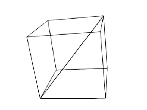
for i=1,2i=1,2 with the center of the bell-shapes at C1=(0.4,0.4,0.4)C_{1}=\left(0.4,0.4,0.4\right), C2=(0.6,0.6,0.6)C_{2}=\left(0.6,0.6,0.6\right), and the radii of the bell-shapes R1=R2=0.2R_{1}=R_{2}=0.2. Figure 4 shows the computational domain with a diagonal line segment and the line plot of the first initial data ψ0​(x→)\psi_{0}\left(\vec{x}\right) along that line segment. Note that the initial data is nonnegative with a compact support. The finite cone of influence [11] enables us to use zero boundary conditions on the unit box Ω=(0,1)×(0,1)×(0,1)\Omega=\left(0,1\right)\times\left(0,1\right)\times\left(0,1\right) as computational domain, since the solution’s domain of support stayed inside the unit box. As second initial data ψ1\psi_{1} we choose a constant multiple of the first initial data

ψ1​(x)=−5​ϕ0​(x)∀x=(x1,x2,x3)∈Ω.\psi_{1}(x)=-5\phi_{0}(x)\qquad\forall x=(x_{1},x_{2},x_{3})\in\Omega.

The parameter values are λ=μ2=0.1\lambda=\mu^{2}=0.1. Initially there is no bubble present. Figure 5 shows the formation and interactions of bubbles. After the two bubbles form around time t=0.08t=0.08, their size grows continuously. Around time t=0.69t=0.69 the two bubbles touch, and from that time on they are attached to each other. At time t=0.8t=0.8 (shown on part (d) of Figure 5) an additional tiny bubble forms inside each of the now merged bubbles. These additional bubbles grow (part (e) of Figure 5 at time t=1t=1); then they flatten and become concave (part (f) of Figure 5 at time t=2t=2). Later hole forms in them and they become toroidal (part (g) of Figure 5 at time t=2.15t=2.15), and finally they disappear (part (h) of Figure 5 at time t=3t=3). The growth of the larger outer bubble exponentially slows down and it does not seem to change shape after time t=3t=3.

Figure 4: Computational domain and first initial data
Computational domain Initial data along a diagonal line segment
Refer to caption Refer to caption
Figure 5: Formation and interaction of two bubbles
(a) 3D bubbles at t=0.08t=0.08 (b) 3D bubbles at t=0.2t=0.2
Refer to caption Refer to caption
(c) 3D bubbles at t=0.69t=0.69 (d) 3D bubbles at t=0.8t=0.8
Refer to caption Refer to caption
(e) 3D bubbles at t=1t=1 (f) 3D bubbles at t=2t=2
Refer to caption Refer to caption
(g) 3D bubbles at t=2.15t=2.15 (h) 3D bubbles at t=3t=3
Refer to caption Refer to caption

Acknowledgments

The authors acknowledge the Texas Advanced Computing Center at The University of Texas at Austin for providing high performance computing and visualization resources that have contributed to the research results reported within this paper. URL: http://www.tacc.utexas.edu. We also gratefully acknowledge the support of NVIDIA Corporation with the donation of the Tesla K40 GPU used for this research. K.Y. was supported by University of Texas Rio Grande Valley College of Sciences 2016-17 Research Enhancement Seed Grant.

References

  • [1] H. Bateman,  A. Erdelyi,  Higher Transcendental Functions. vol. 1,2, New York: McGraw-Hill, 1953.
  • [2] A. Bers, R. Fox, C. G Kuper, S. G. Lipson, The impossibility of free tachyons, in Relativity and Gravitation, eds. C. G. Kuper and Asher Peres, New York, Gordon and Breach Science Publishers, 1971, 41–46.
  • [3] S. Coleman,  Aspects of Symmetry: Selected Erice Lectures. Cambridge University Press, 1985.
  • [4] K. Dekker, J.G. Verwer,  Stability of Runge-Kutta methods for Stiff Nonlinear Differential Equations., North-Holland, Amsterdam: Elsevier Science Ltd., 1984.
  • [5] H. Epstein, U. Moschella, de Sitter tachyons and related topics. Comm. Math. Phys. 336 (1)  (2015) 381–430
  • [6] A. Galstian, K. Yagdjian, Global in time existence of self-interacting scalar field in de Sitter space-times. Nonlinear Analysis: Real World Applications 34 (2017) 110–139.
  • [7] J. Ginibre,, G. Velo,  The global Cauchy problem for the nonlinear Klein-Gordon equation. Math. Z. 189, no. 4: (1985) 487–505.
  • [8] J. Ginibre, G. Velo,  The global Cauchy problem for the nonlinear Klein-Gordon equation. II. Ann. Inst. H. Poincaré Anal. Non Linéaire. 6, no. 1 (1989) 15–35.
  • [9] S. W. Hawking, G. F. R. Ellis, The large scale structure of space-time. Cambridge Monographs on Mathematical Physics, No. 1. London-New York: Cambridge University Press, 1973.
  • [10] P.W. Higgs, Broken symmetries and the masses of gauge bosons.  Phys. Rev. Lett. 13, no. 16 (1964) 508–509.
  • [11] L. Hörmander,   Lectures on nonlinear hyperbolic differential equations. Berlin:  Springer-Verlag, 1997.
  • [12] H.B. Keller, V. Pereyra, Symbolic generation of finite difference formulas. Math. Comp. 32 (144) (1978) 955–971.
  • [13] S. Klainerman, Global existence for nonlinear wave equations. Comm. Pure Appl. Math. 33 , no. 1 (1980) 43–101.
  • [14] T.D. Lee,  G.C. Wick,  Vacuum stability and Vacuum Excitation in Spin-0 Field.   Phys. Rev. D 9 (8) (1974) 2291–2316.
  • [15] A. Linde,  Particle Physics and Inflationary Cosmology. Harwood, Chur, Switzerland, 1990.
  • [16] C. Møller,  The theory of relativity. Oxford: Clarendon Press, 1952.
  • [17] M.H. Protter, H.F. Weinberger,  Maximum Principles in Differential Equations. by Springer-Verlag New York Inc., 1984
  • [18] NVIDIA Corporation: PGI CUDA Fortran Compiler.  (2017)
  • [19] A. Rendall,   Partial differential equations in general relativity. Oxford Graduate Texts in Mathematics, 16, Oxford: Oxford University Press, 2008.
  • [20] D. Sather, A maximum property of Cauchy’s problem for the wave operator. Arch. Rational Mech. Anal. 21 (1966) 303–309.
  • [21] J. Shatah, M. Struwe, Geometric wave equations. Courant Lect. Notes Math., 2. New York Univ., New York: Courant Inst. Math. Sci., 1998.
  • [22] S. Sonego, V. Faraoni, Huygens’ principle and characteristic propagation property for waves in curved space-times. J. Math. Phys. 33 , no. 2 (1992) 625–632.
  • [23] G. Strang,   Computational science and engineering. Wellesley, MA: Wellesley-Cambridge Press, 2007.
  • [24] J. Speck, Finite-time degeneration of hyperbolicity without blowup for quasilinear wave equations, Analysis&PDE, 10, no. 8 (2017) 2001–2030.
  • [25] A. Vasy, The wave equation on asymptotically de Sitter-like spaces.   Adv. Math. 223, no. 1 (2010) 49–97.
  • [26] N.A. Voronov, A.L. Dyshko, , N.B. Konyukhova, On the Stability of a Self-Similar Spherical Bubble of a Scalar Higgs Field in de Sitter Space.   Physics of Atomic Nuclei 68, no. 7: (2005) 1218–1226.
  • [27] A. Weinstein,   On a Cauchy problem with subharmonic initial values. Ann. Mat. Pura Appl. (4) 43 (1957) 325–340.
  • [28] K. Yagdjian, Global existence in the Cauchy problem for nonlinear wave equations with variable speed of propagation, New trends in the theory of hyperbolic equations, Oper. Theory Adv. Appl., 159, Birkhäuser, Basel, (2005) 301–385.
  • [29] K. Yagdjian, A. Galstian,  Fundamental Solutions for the Klein-Gordon Equation in de Sitter space-time,  Comm. Math. Phys. 285 (2009) 293–344.
  • [30] K. Yagdjian, The semilinear Klein-Gordon equation in de Sitter space-time, Discrete Contin. Dyn. Syst. Ser. S 2 (3) (2009) 679–696.
  • [31] K. Yagdjian,  On the global solutions of the Higgs boson equation, Comm. Partial Differential Equations  37 (3)  (2012) 447–478.
  • [32] K. Yagdjian,  Global existence of the scalar field in de Sitter space-time, J. Math. Anal. Appl. 396 (1) (2012) 323–344.
  • [33] K. Yagdjian,  Huygens’ Principle for the Klein-Gordon equation in the de Sitter space-time, J. Math. Phys.   54, no. 9 (2013) 091503.
  • [34] K. Yagdjian, Integral transform approach to solving Klein-Gordon equation with variable coefficients, Mathematische Nachrichten, 288 (17-18) (2015) 2129-2152.
  • [35] K. Yagdjian, Global existence of the self-interacting scalar field in the de Sitter universe, arXiv:1706.07703