Asymptotic coverage probabilities of bootstrap percentile confidence intervals for constrained parameters

We first consider the one-sample problem with a linear inequality constraint on the mean parameter space. Suppose $X_{1},\ldots,X_{n}$ is a random sample from a general parametric distribution in the natural exponential family with probability density function or probability mass function

where $\psi$ is the natural parameter, and $\theta=E(X_{1})=b^{\prime}(\psi)$ represents the mean parameter. It is assumed that $b(\cdot)$ is twice continuously differentiable with $b^{\prime\prime}(\psi)>0$. Let $\sigma^{2}=b^{\prime\prime}(\psi)$ be the variance of $X_{1}$ under $f(x;\theta)$. The parameter space of $\theta$ is constrained in $\mathcal{C}_{1}=\{\theta:\theta\geq d\}$ for some fixed boundary $d$. We aim to quantify the coverage probability of the bootstrap percentile confidence interval for $\theta$.

Based on $n$ random observations from (2.1), the log-likelihood function of $\theta$, up to a constant not dependent on $\theta$, is $l_{n}(\theta)=\psi\sum_{i=1}^{n}X_{i}-nb(\psi).$ Then the maximum likelihood estimator of $\theta$ is defined as $\hat{\theta}_{n}=\arg\max_{\theta\in\mathcal{C}_{1}}l_{n}(\theta).$ The following lemma finds the closed form of $\hat{\theta}_{n}$.

Next, we construct the bootstrap percentile confidence interval of $\theta$ based on $\hat{\theta}_{n}$. Let $X_{1}^{*},\ldots,X_{n}^{*}$ denote a parametric bootstrap sample from the model $f(x;\hat{\theta}_{n})$, for given $\hat{\theta}_{n}$, and let $\hat{\theta}^{*}_{n}=\max(\bar{X}_{n}^{*},d)$ denote the maximum likelihood estimator of $\theta$ based on the bootstrap sample, where $\bar{X}_{n}^{*}=\sum_{i=1}^{n}X_{i}^{*}/n$. Further, let $G_{n}^{*}(x;\hat{\theta}_{n})={\mbox{\rm pr}}(\hat{\theta}_{n}^{*}\leq x\mid\hat{\theta}_{n})$ be the bootstrap distribution function of ${\hat{\theta}_{n}}$, and $q^{*}_{\alpha}$ be the $\alpha$-quantile of $G_{n}^{*}(x;\hat{\theta}_{n})$. Then $[q^{*}_{\alpha_{1}},q^{*}_{1-\alpha_{2}}]$ is called a nominally $100(1-\alpha)\%$ level bootstrap percentile confidence interval of $\theta$, and its coverage probability is defined to be

where $\theta_{0}$ is the true value of $\theta$, $\alpha=\alpha_{1}+\alpha_{2}$ with $\alpha_{1},\alpha_{2}\in(0,0.5)$, and ${\mbox{\rm pr}}(\cdot)$ indicates the probability under $f(x;\theta_{0})$.

Under the general parametric model setup, the explicit form of the coverage probability of the bootstrap percentile confidence interval of $\theta$ is typically unavailable, or has to be derived case by case. Therefore, it is of interest to quantify the asymptotic coverage probability of the bootstrap percentile confidence interval for $\theta$ as $n\to\infty$.

Our asymptotic framework is motivated by a simple, but generic, example discussed in Andrews (1997); Andrews (2000).

We comment that the exact coverage probability in (2.1) is a piecewise constant function of $\theta_{0}$ with a step change at $n^{-1/2}\Phi^{-1}(1-\alpha_{2})$, for given $n$ and $\alpha_{2}$ values. Also, from (2.1), we can see that the coverage for $\theta$ depends on how close the true value $\theta_{0}$ is to the boundary. The magnitude of closeness of $\theta_{0}$ to the boundary crucially depends on the sample size by an order of ${n}^{1/2}$.

As an illustration, Figure 2(a) plots the exact coverage probabilities versus the true value of $\theta_{0}$ for different sample sizes $n$ at level $1-\alpha=0.90$ with $\alpha_{1}=\alpha_{2}=\alpha/2$. We see that the bootstrap percentile confidence interval may behave conservatively in terms of its coverage. Specifically, when the true value $\theta_{0}$ is on, or close to, the boundary, over-coverage can happen. To further verify the trend that we have seen for the normal example, recall that, in Figure 1(a), we also plot the exact coverage probability of the bootstrap percentile confidence interval for the rate parameter $\lambda$ of Poisson distribution with $\lambda\geq 2$ at level $1-\alpha=0.90$ with $\alpha_{1}=\alpha_{2}=\alpha/2$ for $n=400$. Due to the discrete nature of the Poisson distribution, we can not always expect the exact coverage probability to achieve the nominal level. Hence, we would hope to more appropriately quantify the observed exact coverage phenomenon in an asymptotically meaningful way.

Motivated by above discussions, we adopt a local asymptotic framework by allowing the true constrained parameter to vary in a $n^{-1/2}$-neighbourhood of the boundary. More precisely, we let $\theta_{0}=\theta_{0,n}=d+\tau n^{-1/2}$. The corresponding local parameter $\tau=n^{1/2}(\theta_{0,n}-d)$ controls the order of closeness of $\theta_{0,n}$ approaching to the boundary $d$. This framework helps capture the subtle asymptotic coverage behaviour of the bootstrap percentile confidence interval in terms of $\tau$ for the general distributions in the natural exponential family with a constrained parameter space.

Under the local asymptotic framework proposed in Section 2.2, we first study the asymptotic distribution of the maximum likelihood estimator $\hat{\theta}_{n}$.

Using Lemmas 2.1 and 2.2, we quantify the local asymptotic coverage probability of bootstrap percentile confidence interval for $\theta$ in the following theorem.

This asymptotic result generalizes the exact finite sample result in Example 2.1 for the normal distribution to cover the natural exponential family of distributions. The result is plotted in Figure 2(b) versus the local parameter $\tau$ at level $1-\alpha=0.90$ with $\alpha_{1}=\alpha_{2}=0.05$ and $\sigma_{0}=1$. We note that different choices of $\alpha_{1}$ and $\alpha_{2}$ should give different graphs. If such an approximation remains good for finite $n$, then this local asymptotic result provides us with information on how likely we are to have conservative conclusions, when $\theta_{0,n}$ is shrinking close to $d$.

In Section 2.3, we quantified the local asymptotic coverage probabilities of bootstrap percentile confidence intervals for boundary constrained parameters when the data come from the general class of distributions in the natural exponential family. In many applications, as seen in the introduction, observations may come from specific parametric distributions, such as Poisson or binomial, in which their mean parameters are subject to linear inequality constraints. To make the asymptotic result of Theorem 2.1 practically useful, we illustrate with two examples in this section. In these examples, we compare the exact coverage probabilities calculated under specific parametric models and the quantified asymptotic coverage probabilities.

In this section, we consider the two-sample problem when data come from general distributions in the natural exponential family with their means subject to a linear ordering constraint. Suppose we have random observations $X_{11},\ldots,X_{1n_{1}}$ from $f(x;\theta_{1})$, and independently, we have random observations $X_{21},\ldots,X_{2n_{2}}$ from $f(x;\theta_{2})$, where $f(x;\theta_{i})$ satisfies (2.1) and $\theta_{i}$ still represents the mean parameter, $i=1,2$. The parameter space of $(\theta_{1},\theta_{2})$ is defined to be $\mathcal{C}_{2}=\{(\theta_{1},\theta_{2}):\theta_{1}\leq\theta_{2}\}$. Our goal is to quantify the asymptotic coverage probabilities of bootstrap percentile confidence intervals for $\theta_{1}$, $\theta_{2}$, as well as their difference $\Delta:=\theta_{2}-\theta_{1}$.

As a first step, we identify the form of the maximum likelihood estimator of $(\theta_{1},\theta_{2},\Delta)$. For an asymptotic analysis, we let $\omega=n_{1}/n$ with $n=n_{1}+n_{2}$ and assume that $\omega\in(0,1)$ does not depend on $n$. The following lemma finds the explicit forms of the maximum likelihood estimators of $\theta_{1}$, $\theta_{2}$ and $\Delta$.

Similarly to the discussion in Section 2.2, fixing $(\theta_{10},\theta_{20})$ and $\Delta_{0}$ pointwisely may not be helpful to reveal the subtle asymptotic coverage behaviour of the bootstrap percentile confidence intervals. Instead we proceed by considering the following local asymptotic framework:

where $\Delta_{0,n}=\delta n^{-1/2}$. Here $\eta_{0}$ is a fixed value, and $\delta$ is a fixed, nonnegative, local parameter not depending on $n$. Under this framework, we fix the true value of $\omega\theta_{10,n}+(1-\omega)\theta_{20,n}$, i.e. the overall mean of two samples, to be $\eta_{0}$, and allow the true value of constrained mean difference, $\Delta_{0,n}=\theta_{20,n}-\theta_{10,n}$, to vary in a $n^{-1/2}$-neighbourhood of 0.

Under this proposed local asymptotic framework, we next study the asymptotic distributions of the maximum likelihood estimators $\hat{\theta}_{n1}$, $\hat{\theta}_{n2}$ and $\hat{\Delta}_{n}$ in the following lemma.

Let $X_{ij}^{*}$’s be the bootstrap sample such that $X_{11}^{*},\ldots,X_{1n_{1}}^{*}$ is a random sample from $f(x;\hat{\theta}_{n1})$ for given $\hat{\theta}_{n1}$, and independently, $X_{21}^{*},\ldots,X_{2n_{2}}^{*}$ is a random sample from $f(x;\hat{\theta}_{n2})$ for given $\hat{\theta}_{n2}$. Define $\bar{X}_{ni}^{*}=\sum_{j=1}^{n_{i}}X_{ij}^{*}/n_{i}$, $i=1,2$. Further, let

and $\hat{\Delta}_{n}^{*}=(\bar{X}_{n2}^{*}-\bar{X}_{n1}^{*})^{+}$ be the maximum likelihood estimators of $\theta_{1}$, $\theta_{2}$ and $\Delta$, respectively, based on the bootstrap sample. Denote the bootstrap distributions of $\hat{\theta}_{n1}$, $\hat{\theta}_{n2}$ and $\hat{\Delta}_{n}$, respectively, by

and their $\alpha$-quantiles by $q_{1,\alpha}^{*}$, $q_{2,\alpha}^{*}$ and $q_{\Delta,\alpha}^{*}$.

Further, let $\Phi_{(\mbox{\boldmath\scriptsize$\mu$},\mbox{\scriptsize\boldmath$\Sigma$})}(x,y)$ denote the joint cumulative distribution function of a bivariate normal random vector with mean vector $\mu$ and variance-covariance matrix $\Sigma$, and let $F_{12}(x,y)$ denote the joint cumulative distribution function of

and

That is, based on Lemma 3.2, $F_{12}(x,y)$ is the joint limiting distribution of of $n^{1/2}(\hat{\theta}_{n1}-\theta_{10,n})/\sigma_{0}$ and $n^{1/2}(\hat{\theta}_{n2}-\theta_{20,n})/\sigma_{0}.$ Also, define matrices

In the next theorem, we quantify the local asymptotic coverage probabilities of the bootstrap percentile confidence intervals for $\theta_{1}$, $\theta_{2}$ and $\Delta$.

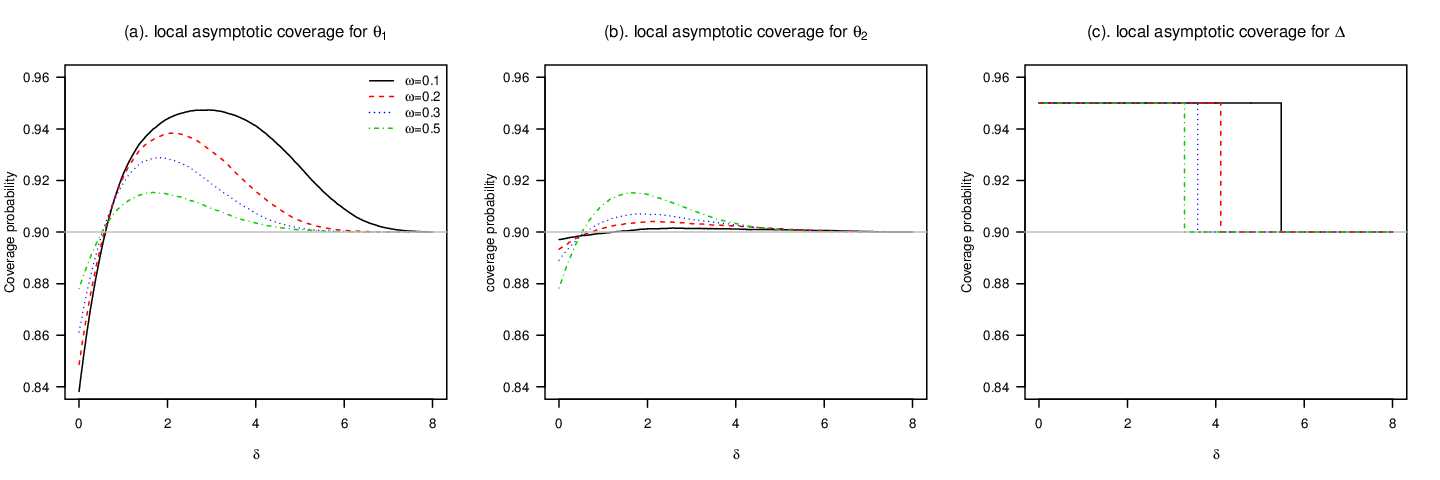
It appears that explicit expressions for the local asymptotic coverage probabilities of $\theta_{1}$ and $\theta_{2}$ are not available. Fortunately, the quantified coverage probabilities of $\theta_{1}$ and $\theta_{2}$ are written in terms of bivariate integrals that can be easily evaluated using numerical methods. Moreover, we note that the asymptotic coverage results only depend on the ratio $\omega$ and the local parameter $\delta$ which actually controls the true mean difference $\Delta_{0,n}$. Figure 5 plots the asymptotic coverage probabilities for $\theta_{1}$, $\theta_{2}$ and $\Delta$ versus the local parameter $\delta$, in the case of $\omega=0.1,0.2,0.3$ and $0.5$ at level $1-\alpha=0.90$ with $\alpha_{1}=\alpha_{2}=0.05$ as an illustration. Again, we note that different choices of $\alpha_{1}$ and $\alpha_{2}$ can lead to different coverage behaviours of the confidence intervals, and hence give different graphs.

From Figure 5, we observe that the asymptotic coverage probabilities for $\theta_{1}$ and $\theta_{2}$ can be, somewhat surprisingly, both greater and smaller than the nominal level. These asymptotic results show that the bootstrap percentile confidence intervals of $\theta_{1}$ and $\theta_{2}$ are no longer always conservative, but can significantly under-cover the corresponding true parameters when the constrained parameter is on, or close to, the restriction boundary. On the other hand, when the two-sample mean difference $\Delta$ is the parameter of interest, the bootstrap percentile confidence interval of $\Delta$ still performs conservatively.

To make our asymptotic results practically appealing, we also apply the results of Theorem 3.1 to a two-sample binomial example with ordered proportions.

Recall that the parameter space for $\theta$ is $\mathcal{C}_{1}=\{\theta:\theta\geq d\}$, which is a closed convex set. Then by Proposition 2.4.3 in Silvapulle and Sen (2004, p. 51), $\hat{\theta}_{n}$ equivalently minimizes

subject to the constraint set $\mathcal{C}_{1}$. That is

This finishes the proof of Lemma 2.1.

Recall that, under the proposed local asymptotic framework, $\theta_{0,n}=d+n^{-1/2}\tau$ and $\sigma_{0}^{2}=b^{\prime\prime}(\psi_{0})$ with $\psi_{0}=b^{\prime-1}(d)$. Applying the central limit theorem for a triangular array gives

in distribution, as $n\to\infty$, where $\sigma_{n}^{2}=b^{\prime\prime}(\psi_{n})$ with $\psi_{n}=b^{\prime-1}(\theta_{0,n})$ and $Z\sim N(0,1)$. Further, both $b^{\prime-1}(\cdot)$ and $b^{\prime\prime}(\cdot)$ are continuous functions, and $\theta_{0,n}\to d$ as $n\to\infty$. Then we have $\sigma_{n}^{2}\to\sigma_{0}^{2}$ as $n\to\infty$. By Slutsky’s theorem, we have

in distribution, as $n\to\infty$. Together with the continuous mapping theorem, it follows that

in distribution, as $n\to\infty$. This completes the proof of Lemma 2.2.

We first recall some notation. Let $X_{1}^{*},\ldots,X_{n}^{*}$ be the bootstrap sample from $f(x;\hat{\theta}_{n})$ for the given $\hat{\theta}_{n}$, and $\hat{\theta}_{n}^{*}=\max(\bar{X}_{n}^{*},d)$ be the maximum likelihood estimator of $\theta$ based on the bootstrap sample, where $\bar{X}_{n}^{*}=\sum_{i=1}^{n}X_{i}^{*}/n.$ Denote the bootstrap distributions of $\hat{\theta}_{n}$ and $\bar{X}_{n}$, respectively, by

Then

Recall that $q_{\alpha}^{*}$ is the $\alpha^{\rm th}$ quantile of the bootstrap distribution of $\hat{\theta}_{n}$. It follows that

Therefore

Let

which is the bootstrap distribution of the standardized $\bar{X}_{n}$. Then

Therefore

We next study the asymptotic property of $\bar{H}_{n}^{*-1}(\alpha_{1};\hat{\theta}_{n})$ in the following lemma, which is very helpful in our proofs.

We first consider Part (a). Note that (4.1) implies that $\bar{X}_{n}-\theta_{0,n}=o_{p}(1)$. Recall that $\theta_{0,n}=d+n^{-1/2}\tau$. Then

References

• Andrews (1997) [author] Andrews, Donald W. K.D. W. K. (1997). A simple counterexample to the bootstrap Cowles Foundation discussion paper 1157, Cowles Foundation for Research in Economics, Yale University.
• Andrews (2000) [author] Andrews, Donald W. K.D. W. K. (2000). Inconsistency of the bootstrap when a parameter is on the boundary of the parameter apace. Econometrica 68 399–405. 10.1111/1468-0262.00114
• Andrews (2001) [author] Andrews, Donald W. K.D. W. K. (2001). Testing when a parameter is on the boundary of the maintained hypothesis. Econometrica 69 683–734. 10.1111/1468-0262.00210
• Barlow et al. (1972) [author] Barlow, Richard ER. E., Bartholomew, David JD. J., Bremner, JMJ. and Brunk, H DanielH. D. (1972). Statistical Inference under Order Restrictions: the Theory and Application of Isotonic Regression. John Wiley & Sons, New York.
• Cheng (2015) [author] Cheng, GuangG. (2015). Moment consistency of the exchangeably weighted bootstrap for semiparametric M-estimation. Scandinavian Journal of Statistics 42 665–684. 10.1111/sjos.12128
• Chernoff (1954) [author] Chernoff, HermanH. (1954). On the Distribution of the Likelihood Ratio. The Annals of Mathematical Statistics 25 573-578.
• Davison and Hinkley (1997) [author] Davison, Anthony ChristopherA. C. and Hinkley, David VictorD. V. (1997). Bootstrap Methods and Their Application. Cambridge University Press, Cambridge.
• Drton and Williams (2011) [author] Drton, MathiasM. and Williams, BenjaminB. (2011). Quantifying the failure of bootstrap likelihood ratio tests. Biometrika 98 919-934. 10.1093/biomet/asr033
• Efron and Tibshirani (1993) [author] Efron, BradleyB. and Tibshirani, Robert J.R. J. (1993). An Introduction to the Bootstrap. Chapman and Hall, New York.
• Feldman and Cousins (1998) [author] Feldman, Gary J.G. J. and Cousins, Robert D.R. D. (1998). Unified approach to the classical statistical analysis of small signals. Physical Review D 57 3873–3889. 10.1103/PhysRevD.57.3873
• Hall (1988) [author] Hall, PeterP. (1988). Theoretical comparison of bootstrap confidence intervals (with Discussion). The Annals of Statistics 16 927-953.
• Hall (1992) [author] Hall, PeterP. (1992). The Bootstrap and Edgeworth Expansion. Springer-Verlag, New York.
• Lee (1994) [author] Lee, Stephen Man SingS. M. S. (1994). Optimal choice between parametric and non-parametric bootstrap estimates. Mathematical Proceedings of the Cambridge Philosophical Society 115 335–363. 10.1017/S0305004100072121
• Li, Taylor and Nan (2010) [author] Li, ZhiguoZ., Taylor, Jeremy M. G.J. M. G. and Nan, BinB. (2010). Construction of Confidence Intervals and Regions for Ordered Binomial Probabilities. The American Statistician 64 291–298. 10.1198/tast.2010.09096
• Molenberghs and Verbeke (2007) [author] Molenberghs, GeertG. and Verbeke, GeertG. (2007). Likelihood Ratio, Score, and Wald Tests in a Constrained Parameter Space. The American Statistician 61 22–27. 10.1198/000313007X171322
• Robertson, Wrigth and Dykstra (1988) [author] Robertson, TimT., Wrigth, F. T.F. T. and Dykstra, Richard L.R. L. (1988). Order Restricted Statistical Inference. John Wiley & Sons, New York.
• Self and Liang (1987) [author] Self, Steven G.S. G. and Liang, Kung-YeeK.-Y. (1987). Asymptotic Properties of Maximum Likelihood Estimators and Likelihood Ratio Tests under Nonstandard Conditions. Journal of the American Statistical Association 82 605–610. 10.1080/01621459.1987.10478472
• Shao and Tu (1995) [author] Shao, JunJ. and Tu, DongshengD. (1995). The Jackknife and Bootstrap. Springer-Verlag, New York.
• Silvapulle and Sen (2004) [author] Silvapulle, Mervyn J.M. J. and Sen, Pranab KumarP. K. (2004). Constrained Statistical Inference: Inequality, Order, and Shape Restrictions 912. John Wiley & Sons, New York.
• van der Vaart (1998) [author] van der Vaart, Aad WA. W. (1998). Asymptotic Statistics. Cambridge University Press, Cambridge.