跳到论文正文
W Papers独立论文阅读器 arXiv:1712.02352 论文正文 计算阅读时间 · 0%
引用这篇论文根据当前论文元数据生成,正式投稿前建议核对。


License: arXiv.org perpetual non-exclusive license
arXiv:1712.02352v2 [cond-mat.supr-con] 02 Apr 2018

Topology from Triviality

V. Kaladzhyan Email: vardan.kaladzhyan@phystech.edu Affiliation: Institut de Physique Théorique, Université Paris Saclay, CEA CNRS, Orme des Merisiers, 91190 Gif-sur-Yvette Cedex, France Affiliation: Laboratoire de Physique des Solides, CNRS, Univ. Paris-Sud, Université Paris-Saclay, 91405 Orsay Cedex, France Affiliation: Department of Physics, KTH Royal Institute of Technology, Stockholm, SE-106 91 Sweden Affiliation: Moscow Institute of Physics and Technology, Dolgoprudny 141700, Moscow region, Russia    Cristina Bena Affiliation: Institut de Physique Théorique, Université Paris Saclay, CEA CNRS, Orme des Merisiers, 91190 Gif-sur-Yvette Cedex, France    Pascal Simon Affiliation: Laboratoire de Physique des Solides, CNRS, Univ. Paris-Sud, Université Paris-Saclay, 91405 Orsay Cedex, France
August 24, 2026
Abstract

We show that bringing into proximity two topologically trivial systems can give rise to a topological phase. More specifically, we study a 1D metallic nanowire proximitized by a 2D superconducting substrate with a mixed ss-wave and pp-wave pairing, and we demonstrate both analytically and numerically that the phase diagram of such a setup can be richer than reported before. Thus, apart from the two ”expected” well-known phases (i.e., where the substrate and the wire are both simultaneously trivial or topological), we show that there exist two peculiar phases in which the nanowire can be in a topological regime while the substrate is trivial, and vice versa.

I Introduction

The last decade was marked by numerous proposals to realize time-reversal-symmetric (TRS) topological superconductors [1, 2, 3, 4, 5, 6, 7, 8, 9, 10, 11, 12, 13] hosting so-called Majorana Kramers pairs. Despite the fact that all the braiding operations in such systems are bound to be performed with pairs rather than with single Majorana quasiparticles, it has been proposed theoretically that braiding of end states remains non-Abelian due to the protection by time reversal symmetry [8].

Certain recipes for creating TRS topological superconductivity (SC) are of high relevance to the current manuscript. First, it is known that a metallic nanowire (NW) proximitized by a SC becomes superconducting due to the proximity effect. Moreover, when the substrate is topological, Majorana fermions may form in the wire [14]. Furthermore, as shown in Ref. [15], a NW proximitized by a helical pp-wave SC substrate becomes a 1D TRS topological SC exhibiting triplet pairing and Majorana Kramers pairs at its ends. It was also demonstrated in [8] that if the SC substrate is characterized by a mixed singlet-triplet pairing with a dominant triplet component, then the NW becomes topological.

Second, in a recent paper, Neupert et al. considered a chain of scalar impurities immersed into a superconductor with a mixed ss-wave and pp-wave order parameter [16]. Scalar impurities do not give rise to Yu-Shiba-Rusinov states [17, 18, 19] in purely ss-wave SCs, in accordance with the Anderson theorem [20]. However, in the presence of a pp-wave pairing component, a pair of in-gap bound states is formed in the presence of a scalar impurity[21, 22, 23]. Given a chain of such impurities, the corresponding bound states hybridize into a so-called ”Shiba band”. As shown in Ref. [16], such a band can enter a topological regime, supporting Majorana bound states at its ends, even though the superconductor is in a trivial phase with a dominant ss-wave component.

Furthermore, Hsieh et al. demonstrated that topological phases can be induced in trivial systems via coupling to topological ones, despite the absence of a local order parameter in the latter. One of the examples in their paper [24] focuses on how a trivial system coupled to a Chern insulator in a topological regime with Chern number −1-1 becomes topological with an opposite Chern number, +1+1. The authors also proposed an analogous example with two coupled 1D systems instead of 2D ones.

Refer to caption
Figure 1: (Color online) A sketch of the system: a metallic nanowire (violet) on top of a 2D SC substrate with mixed singlet and triplet pairing (blue). Red arrows denote the tunnelling between the substrate and the wire, and the Majorana Kramers pairs are drawn as yellow spheres at the ends of the wire.

Motivated by the aforementioned findings, we offer in this paper another missing piece of the puzzle. In what follows we show that bringing into proximity two topologically trivial systems can give rise to a topological phase. We exemplify this idea by studying a 1D metallic NW proximitized by a 2D SC substrate with a mixed ss-wave and pp-wave pairing (see Fig. 1). We obtain the phase diagram of the system in Fig. 1 using both analytical and numerical methods. The analytical approach is based on integrating out the SC degrees of freedom and obtaining an effective low-energy Hamiltonian for the nanowire, whereas the numerical simulations are done within a tight-binding model on a square lattice. The phase diagrams are constructed by testing the formation of Majorana bound states at the ends of the nanowire.

The resulting phase diagrams recover first the two phases that have also been previously reported [15, 8]: one in which both the substrate and the nanowire are trivial, as well as one in which both are topological. However, they exhibit also two salient unexpected phases which have never been discussed before. Thus we identify a phase in which the SC is topological, whereas the induced superconductivity in the NW is trivial. Also, most surprisingly, one can achieve a phase in which the SC substrate is trivial whereas the NW is topological.

II Continuum model

We start by considering a 1D metallic NW oriented along the xx axis and deposited on top of a 2D TRS SC with both ss-wave and pp-wave pairing, lying in the (x,y)(x,y) plane. The Hamiltonian of the NW is given by

ℋNW=(px22​m−μ)​σ0⊗τz,\mathcal{H}_{\mathrm{NW}}=\left(\frac{p_{x}^{2}}{2m}-\mu\right)\sigma_{0}\otimes\tau_{z}, (1)

and the Hamiltonian of the superconducting substrate can be written as

ℋSC=𝒑2−pF22​M​σ0⊗τz+Δs​σ0⊗τx+ϰ⁡(py​σx−px​σy)⊗τx.\mathcal{H}_{\mathrm{SC}}=\frac{\bm{p}^{2}-p_{F}^{2}}{2M}\sigma_{0}\otimes\tau_{z}+\Delta_{s}\sigma_{0}\otimes\tau_{x}+\varkappa(p_{y}\sigma_{x}-p_{x}\sigma_{y})\otimes\tau_{x}. (2)

We use the Nambu bases {cpx↑,cpx↓,c−px↓†,−c−px↑†}T\left\{c_{p_{x}\uparrow},c_{p_{x}\downarrow},c^{{\dagger}}_{-p_{x}\downarrow},-c^{{\dagger}}_{-p_{x}\uparrow}\right\}^{\trans} where cpx↑c_{p_{x}\uparrow} destroys an electron of spin ↑\uparrow with momentum pxp_{x} in the NW, and {Ψ𝒑↑,Ψ𝒑↓,Ψ−𝒑↓†,−Ψ−𝒑↑†}T\left\{\Psi_{\bm{p}\uparrow},\Psi_{\bm{p}\downarrow},\Psi^{{\dagger}}_{-\bm{p}\downarrow},-\Psi^{{\dagger}}_{-\bm{p}\uparrow}\right\}^{\trans} for which Ψ𝒑↑\Psi_{\bm{p}\uparrow} destroys an electron of momentum 𝒑\bm{p} in the substrate. The matrices 𝝈{\bm{\sigma}} and 𝝉{\bm{\tau}} are the Pauli matrices acting respectively in the spin and the particle-hole subspaces. In (1), mm is the effective mass of the quasi-particles in the NW, and μ\mu is their chemical potential. Similarly, in (2), MM and pFp_{F} embody the effective mass of quasi-particles in the SC and their Fermi momentum. The singlet and triplet SC pairings in the substrate are denoted by Δs\Delta_{s} and ϰ\varkappa, respectively. We model the coupling between the NW and the SC by means of a tunnelling Hamiltonian

ℋT=ttun​∑𝒑​σ[Ψ𝒑​σ†​cpx​σ+cpx​σ†​Ψ𝒑​σ],\mathcal{H}_{\trans}=t_{\mathrm{tun}}\sum\limits_{\bm{p}\sigma}\left[\Psi^{\dagger}_{\bm{p}\sigma}c_{p_{x}\sigma}+c^{\dagger}_{p_{x}\sigma}\Psi_{\bm{p}\sigma}\right], (3)

where σ=↑,↓\sigma=\uparrow,\downarrow, and ttunt_{\mathrm{tun}} is the tunnelling amplitude.

In what follows we integrate out the SC degrees of freedom (see Appendix C) and we obtain an effective retarded Green’s function for the proximitized NW:

[GNWeff​(ω,px)]−1=(GNW)−1−∫d​py2​π​ℋT†​GSC​ℋT\left[G^{\mathrm{eff}}_{\mathrm{NW}}\left(\omega,p_{x}\right)\right]^{-1}=\left(G_{\mathrm{NW}}\right)^{-1}-\int\negthickspace\frac{dp_{y}}{2\pi}\mathcal{H}_{\mathrm{T}}^{\dagger}G_{\mathrm{SC}}\mathcal{H}_{\mathrm{T}} (4)

where we defined GNW≡(ω+i​0−ℋNW)−1G_{\mathrm{NW}}\equiv\left(\omega+i0-\mathcal{H}_{\mathrm{NW}}\right)^{-1}, and GSC≡(ω+i​0−ℋSC)−1.G_{\mathrm{SC}}\equiv\left(\omega+i0-\mathcal{H}_{\mathrm{SC}}\right)^{-1}. The effective Green’s function given by Eq. (4) yields an effective low-energy Hamiltonian describing the NW (see, e.g., Ref. [15]):

ℋNWeff≡−(GNWeff)−1|,ω=0\mathcal{H}^{\mathrm{eff}}_{\mathrm{NW}}\equiv-\left(G^{\mathrm{eff}}_{\mathrm{NW}}\right)^{-1}\left|{}_{\omega=0}\right., (5)

where we keep all the terms up to those linear in pxp_{x}. It is worth mentioning that setting the frequency to zero in Eq. (5) is an approximation that allows us to extract a qualitative effective Hamiltonian for the NW. More accurate results can be obtained from an exact diagonalization of the full lattice model, however, as we will show in what follows, the two methods yield consistent results.

Results. We leave the detailed presentation of the tedious calculations for Appendix C, and we present here the first result of this paper – an effective low-energy Hamiltonian for the NW:

HNWeff=(px22​m−μind)​σ0⊗τz−λind​px​σy⊗τz+\displaystyle H_{\mathrm{NW}}^{\mathrm{eff}}=\left(\frac{p_{x}^{2}}{2m}-\mu^{\mathrm{ind}}\right)\sigma_{0}\otimes\tau_{z}-\lambda^{\mathrm{ind}}\,p_{x}\sigma_{y}\otimes\tau_{z}+
+Δsindσ0⊗τx−ϰindpxσy⊗τx.\displaystyle+\Delta_{s}^{\mathrm{ind}}\,\sigma_{0}\otimes\tau_{x}-\varkappa^{\mathrm{ind}}\,p_{x}\sigma_{y}\otimes\tau_{x}.\phantom{aaa} (6)

As a result of the interplay between the ss-wave and pp-wave pairing, an effective Rashba-like spin-orbit coupling arises in the NW. We note that for a pure pp-wave or pure ss-wave coupling no such term is generated, provided there is no spin-orbit coupling in the substrate. The induced parameters in Eq. (6) are defined as follows:

Δsind\displaystyle\Delta_{s}^{\mathrm{ind}} ≡\displaystyle\equiv ttun2π​vF∑σ=±Re[sgn⁡Δσ−i​σ​ϰ~1+ϰ~2arctg−|pε|+zσpε2−zσ2]\displaystyle\frac{t_{\mathrm{tun}}^{2}}{\pi v_{F}}\sum\limits_{\sigma=\pm}\re\left[\frac{\sgn\Delta_{\sigma}-i\sigma\tilde{\varkappa}}{1+\tilde{\varkappa}^{2}}\arctg\frac{-|p_{\varepsilon}|+z_{\sigma}}{\sqrt{p_{\varepsilon}^{2}-z_{\sigma}^{2}}}\right]
ϰind\displaystyle\varkappa^{\mathrm{ind}} ≡\displaystyle\equiv ttun2π​vF∑σ=±Re[−σ​sgn⁡Δσ+i​ϰ~1+ϰ~21zσarctg−|pε|+zσpε2−zσ2]\displaystyle\frac{t_{\mathrm{tun}}^{2}}{\pi v_{F}}\sum\limits_{\sigma=\pm}\re\left[\frac{-\sigma\sgn\Delta_{\sigma}+i\tilde{\varkappa}}{1+\tilde{\varkappa}^{2}}\frac{1}{z_{\sigma}}\arctg\frac{-|p_{\varepsilon}|+z_{\sigma}}{\sqrt{p_{\varepsilon}^{2}-z_{\sigma}^{2}}}\right]
λind\displaystyle\lambda^{\mathrm{ind}} ≡\displaystyle\equiv ttun2π​vF∑σ=±Im[−σ+i​ϰ~​sgn⁡Δσ1+ϰ~21zσarctg−|pε|+zσpε2−zσ2]\displaystyle\frac{t_{\mathrm{tun}}^{2}}{\pi v_{F}}\sum\limits_{\sigma=\pm}\im\left[\frac{-\sigma+i\tilde{\varkappa}\sgn\Delta_{\sigma}}{1+\tilde{\varkappa}^{2}}\frac{1}{z_{\sigma}}\arctg\frac{-|p_{\varepsilon}|+z_{\sigma}}{\sqrt{p_{\varepsilon}^{2}-z_{\sigma}^{2}}}\right]
μind\displaystyle\mu^{\mathrm{ind}} ≡\displaystyle\equiv ttun2π​vF∑σ=±Im[i​σ​ϰ~​sgn⁡Δσ−11+ϰ~2arctg−|pε|+zσpε2−zσ2]+\displaystyle\frac{t_{\mathrm{tun}}^{2}}{\pi v_{F}}\sum\limits_{\sigma=\pm}\im\left[\frac{i\sigma\tilde{\varkappa}\sgn\Delta_{\sigma}-1}{1+\tilde{\varkappa}^{2}}\arctg\frac{-|p_{\varepsilon}|+z_{\sigma}}{\sqrt{p_{\varepsilon}^{2}-z_{\sigma}^{2}}}\right]+ (7)
+μ+ttun2π​vF​ln⁡2​Λ1+ϰ~2,\displaystyle\phantom{aaaaaaaaa}+\mu+\frac{t_{\mathrm{tun}}^{2}}{\pi v_{F}}\frac{\logn 2\Lambda}{1+\tilde{\varkappa}^{2}},

where Δσ≡Δs+σ​ϰ​pF\Delta_{\sigma}\equiv\Delta_{s}+\sigma\varkappa p_{F}, ϰ~≡ϰ/vF\tilde{\varkappa}\equiv\varkappa/v_{F}, while pεp_{\varepsilon} and Λ\Lambda are the IR and UV momentum cutoffs, respectively, unavoidable in an effective low-energy theory. Finally, we have zσ=[σ​ϰ​Δs−pF​vF2+i​vF​|Δσ|]​[vF2+ϰ2]−1.z_{\sigma}=[\sigma\varkappa\Delta_{s}-p_{F}v_{F}^{2}+iv_{F}|\Delta_{\sigma}|][v_{F}^{2}+\varkappa^{2}]^{-1}. We note that the induced chemical potential depends weakly on the UV momentum cutoff Λ\Lambda, however, this term can be absorbed into a redefinition of the initial chemical potential μ\mu of the NW. Our results are fully consistent with calculations performed in Ref. [15] in the limit Δs=0\Delta_{s}=0, namely when the substrate is a purely triplet SC.

To find the induced SC gap for the Hamiltonian in Eq. (6) we linearize its spectrum around the two different Fermi momenta emerging due to the non-zero induced spin-orbit coupling. We thus obtain11 1 Even though this value is close to the actual value of the induced gap, we should note that this expression is however an approximation valid only when the spectrum can be linearized.:

Δindeff=minσ=±|Δsind−m​ϰind​(λind−σ​(λind)2+2​μindm)|1+(ϰind)2(λind)2+2​μindm.\displaystyle\Delta^{\mathrm{ind}}_{\mathrm{eff}}=\min\limits_{\sigma=\pm}\frac{\left|\Delta^{\mathrm{ind}}_{s}-m\varkappa^{\mathrm{ind}}\left(\lambda^{\mathrm{ind}}-\sigma\sqrt{(\lambda^{\mathrm{ind}})^{2}+\frac{2\mu^{\mathrm{ind}}}{m}}\right)\right|}{\sqrt{1+\frac{(\varkappa^{\mathrm{ind}})^{2}}{(\lambda^{\mathrm{ind}})^{2}+\frac{2\mu^{\mathrm{ind}}}{m}}}}. (8)

To test the formation of a topological phase in the NW we check first that the induced effective gap value Δeffind\Delta^{\mathrm{ind}}_{\mathrm{eff}} is non-zero, and second, that the Hamiltonian (6) has a localized zero-energy solution. The underlying superconductor is topological when Δs<ϰ​pF\Delta_{s}<\varkappa p_{F} [26] and the NW if |Δsind|<|ϰind​pσ0ind||\Delta^{\mathrm{ind}}_{s}|<|\varkappa^{\mathrm{ind}}p_{\sigma_{0}}^{\mathrm{ind}}| with pσ0ind=m⁡(λind−σ0​(λind)2+2​μindm)p_{\sigma_{0}}^{\mathrm{ind}}=m\left(\lambda^{\mathrm{ind}}-\sigma_{0}\sqrt{(\lambda^{\mathrm{ind}})^{2}+\frac{2\mu^{\mathrm{ind}}}{m}}\right) is the corresponding effective Fermi momentum in the wire, obtained by taking into account also non-zero Rashba spin-orbit coupling λind\lambda^{\mathrm{ind}} and the corresponding split in the band structure. σ0\sigma_{0} is the value of σ\sigma that minimizes the induced gap Δeffind\Delta^{\mathrm{ind}}_{\mathrm{eff}}.

As we will show below, the most important factor in obtaining different topological phases in the wire and in the substrate is the difference between |pσ0ind||p_{\sigma_{0}}^{\mathrm{ind}}| and pFp_{F}. The former depends only weakly on pFp_{F} (see Fig. A1 in Appendix A), but very strongly on μ\mu, which can thus be used as a ”topological knob”.

The induced chemical potential of the NW μind\mu^{\mathrm{ind}} is also affected by the substrate, and depends linearly on the initial chemical potential of the NW μ\mu (see Eq. (7)).

To understand the mechanisms behind the induced phase transition, in Fig. 2, we plot |Δsind|/|ϰind||\Delta_{s}^{\mathrm{ind}}|/|\varkappa^{\mathrm{ind}}| as a function of Δs\Delta_{s} in the substrate, normalized in units of ϰ\varkappa in the substrate. The substrate topological phase transition takes place at Δs/ϰ=pF\Delta_{s}/\varkappa=p_{F}, the Fermi momentum of the substrate, marked by the vertical black dashed line in the plot. Note the interesting discontinuity at Δs/ϰ=pF\Delta_{s}/\varkappa=p_{F}, we are going to discuss it in more detail in what follows.

The critical Δs\Delta_{s} in the substrate corresponding to the topological phase transition in the NW can be determined by finding the points on this graph for which |Δsind|/|ϰind|=|pσ0ind||\Delta_{s}^{\mathrm{ind}}|/|\varkappa^{\mathrm{ind}}|=|p_{\sigma_{0}}^{\mathrm{ind}}|. The dependence of |pσ0ind||p_{\sigma_{0}}^{\mathrm{ind}}| on Δs\Delta_{s} in the substrate is depicted in Fig. 2 by the dashed red lines corresponding to three different chemical potentials in the NW. Note that |pσ0ind||p_{\sigma_{0}}^{\mathrm{ind}}| is almost independent of Δs\Delta_{s}, except for small jump at ϰ​pF\varkappa p_{F}, its main variation is with μ\mu. The critical values at which the NW becomes topological are obtained by taking the intersection points of the two graphs, |Δsind|/|ϰind||\Delta_{s}^{\mathrm{ind}}|/|\varkappa^{\mathrm{ind}}| and |pσ0ind||p_{\sigma_{0}}^{\mathrm{ind}}| (see Fig. 2). We see that by varying μ\mu in the NW we can tune the intersection points and thus the critical Δs\Delta_{s} for which the NW becomes topological and make it smaller or larger than the one in the substrate. A very interesting point to make is that for values of μ\mu yielding an intersection point inside the discontinuity, the two critical Δs\Delta_{s}’s, for the NW and the substrate, are identical.

Figure 2: (Color online) The ratio of induced pairing parameters |Δsind/ϰind||\Delta_{s}^{\mathrm{ind}}/\varkappa^{\mathrm{ind}}|, as a function of Δs/ϰ\Delta_{s}/\varkappa (blue lines). The black dashed vertical line marks the topological phase transition in the substrate. The red dashed lines describe the dependence of |pσ0ind||p_{\sigma_{0}}^{\mathrm{ind}}| on Δs\Delta_{s} for three different values of the chemical potential in the NW. For each value of μ\mu we have indicated the intersection points corresponding to the values of the critical Δs\Delta_{s} in the substrate which would yield a topological phase transition in the NW. Note that the critical Δs\Delta_{s} of the NW can be smaller, larger or equal to that of the substrate. We have set M=1.5,ϰ=2.5,pF=1.1M=1.5,\varkappa=2.5,p_{F}=1.1, and ttun=0.5t_{\mathrm{tun}}=0.5.

Thus, we can see that by tuning μ\mu in the NW we can tune the transition such that we obtain a topological phase in the NW, associated with a trivial phase in the SC. From the above discussion we can conclude that obtaining such a phase is quite a generic feature as long as, in the first place, one can tune pσ0indp_{\sigma_{0}}^{\mathrm{ind}} independently of pFp_{F}. Moreover, pσ0indp_{\sigma_{0}}^{\mathrm{ind}} depends quite strongly on the chemical potential in the NW, and for our chosen parameters we can approximate |pσ0ind|∝μind∝μ|p_{\sigma_{0}}^{\mathrm{ind}}|\propto\sqrt{\mu^{\mathrm{ind}}}\propto\sqrt{\mu}. Thus, except for the very peculiar and most likely improbable situation in which |Δsind|/|ϰind|=Δs/ϰ|\Delta_{s}^{\mathrm{ind}}|/|\varkappa^{\mathrm{ind}}|=\Delta_{s}/\varkappa, and pσ0ind=pFp_{\sigma_{0}}^{\mathrm{ind}}=p_{F}, one would be able to generate the unusual phases with different topological properties for the NW and the substrate.

As mentioned above, the second necessary ingredient to obtain different topological phases in the NW and the substrate is that the discontinuity in the |Δsind|/|ϰind||\Delta_{s}^{\mathrm{ind}}|/|\varkappa^{\mathrm{ind}}| does not cover the entire range of achievable physical values for pσ0indp_{\sigma_{0}}^{\mathrm{ind}}. Unfortunately it is hard to predict its exact dependence on the parameters of the system analytically, but a simple numerical analysis using Eq. (7) from the main text allows to extract its asymptotic behavior. We have found that the absolute value of the jump is almost exactly given by 2/ϰ2/\varkappa, with the larger ϰ\varkappa, the more precise the estimation. Thus increasing the triplet pairing in the substrate may also increase the range in which the NW is topological while the substrate is not.

An interesting note to make is that, by examining Fig. 2, we can see that when the substrate is in a topological regime (i.e. on the left side of the dashed line), none of the pairings in the NW is favored (mathematically speaking, |Δsind/ϰind|≈Δs/ϰ|\Delta_{s}^{\mathrm{ind}}/\varkappa^{\mathrm{ind}}|\approx\Delta_{s}/\varkappa). However, in the trivial regime (i.e. on the right side of the dashed line) we can infer from the slope of the curve that inducing singlet pairing is more favorable than triplet one, and thus we would intuitively expect a trivial phase in the wire in this range. However, as it turns out, pσ0indp_{\sigma_{0}}^{\mathrm{ind}}, and not |Δsind/ϰind||\Delta_{s}^{\mathrm{ind}}/\varkappa^{\mathrm{ind}}| is the most important knob for tuning the phase transition of the NW, and it is its variation that allows us to obtain the non-trivial combination of phases discussed above.

In what follows we construct a phase diagram capturing the topological character of both the SC and the NW. We emphasise that we do not study topological properties of the system ”substrate + nanowire” as a whole, but we study them separately, showing both simultaneously on the phase diagrams. This can be achieved by combining the ℤ2\mathbb{Z}_{2} topological index for the NW and the ℤ2\mathbb{Z}_{2} index for the substrate into a global topological index δ\delta as follows. The topological character of each system is considered separately, by means of a standard criterion mentioned above, i.e. the sign of Δs−κ​pF\Delta_{s}-\kappa p_{F} shows the nature of a given phase. We combine two criteria into one by summing them up and introducing factors 3/23/2 for the substrate and 1/21/2 for the wire, solely for convenience, to distinguish the case of topological substrate and trivial nanowire from that of trivial substrate and topological nanowire (otherwise the sum of topological indices would give 00 in both cases). This combined index δ\delta allows to discriminate between all four different combinations of phases we can possibly expect in our setup, and is thus given by:

δ=32​sgn⁡(Δs−ϰ​pF)+12​sgn⁡(|ϰind​pσ0ind|−|Δsind|).\delta=\frac{3}{2}\sgn\left(\Delta_{s}-\varkappa p_{F}\right)+\frac{1}{2}\sgn\left(|\varkappa^{\mathrm{ind}}p_{\sigma_{0}}^{\mathrm{ind}}|-|\Delta^{\mathrm{ind}}_{s}|\right). (9)

δ\delta can take four different values, corresponding to the four possible phases of the NW-SC systems; these values and the corresponding phases are summarized in Table I. The most exciting phase corresponds to δ=+2\delta=+2, for which a NW can attain a topological phase when proximitized by a trivial SC.

SC NW
δ=+2\delta=+2 trivial topological
δ=+1\delta=+1 trivial trivial
δ=−1\delta=-1 topological topological
δ=−2\delta=-2 topological trivial
Table 1: The four possible topological phases for the NW-SC system.

In Fig. 3 we plot the value of the topological index δ\delta as a function of Δs\Delta_{s} (more precisely as a function of Δsϰ−pF\frac{\Delta_{s}}{\varkappa}-p_{F}), and of μ\mu, when all the other parameters of the model are fixed. We note the formation of all the four possible phases that could be realized in this setup. First two combinations were known and studied before: ”trivial substrate + trivial nanowire” (the yellow phase with δ=+1\delta=+1 in Fig. 3) and ”topological substrate + topological nanowire” (the light blue phase with δ=−1\delta=-1 in Fig. 3). The main observable signature of the latter combination is the local density of states due to the formation of Majorana zero modes at the ends of the nanowire and at the boundary of the substrate. The other two combinations that we discovered and described in our paper correspond to having ”topological substrate + trivial nanowire” (deep blue phase with δ=−2\delta=-2 in Fig. 3) and ”trivial substrate + topological nanowire” (red phase with δ=+2\delta=+2 in Fig. 3). In the former case Majorana bound states will appear solely at the boundary of the substrate, whereas in the latter combination they will form only at the ends of the nanowire. For any set of parameters corresponding to this phase, we can demonstrate that there is a doubly-degenerate localized zero-energy solution, confirming the topological character of the NW. Due to the presence of TRS these Majorana bound states form protected Kramers pairs which are robust to non-magnetic disorder.

Refer to caption
Figure 3: (Color online) The phase diagram of a 1D metallic NW deposited on top of a 2D SC substrate. We plot the value of the topological index δ\delta defined in Eq. (9) as a function of Δsϰ−pF\frac{\Delta_{s}}{\varkappa}-p_{F} in the substrate, and of μ\mu in the NW. We note that all the four possible phases corresponding to δ=±1,±2\delta=\pm 1,\pm 2 can form. The region with δ=+2\delta=+2 (denoted in red) is the most interesting, and corresponds to a topological phase of the NW induced via the proximity of a trivial SC. The black dashed line marks the bulk topological phase transition for the substrate. We have set pF=1.1,M=m=1.5,ϰ=2.5p_{F}=1.1,M=m=1.5,\varkappa=2.5, and ttun=0.5t_{\mathrm{tun}}=0.5.
Refer to caption
Figure 4: (Color online) The phase diagram of a 1D NW of length L=151L=151 deposited on top of a 201×51201\times 51 2D SC substrate. We plot the combined topological index δ\delta, as defined in Table I, as a function of Δs\Delta_{s} and μNW\mu_{\mathrm{NW}} (in units of tt, which we set to 11). The topological character of the NW is obtained by calculating the MP of the lowest-energy states (with a cutoff at 0.9). The dashed line at Δs∼0.86​t\Delta_{s}\sim 0.86t marks the bulk topological phase transition. We set μSC=3,Δt=0.5\mu_{\mathrm{SC}}=3,\Delta_{t}=0.5 and ttun=2t_{\mathrm{tun}}=2 .

III Lattice model

Hereinafter, we consider a tight-binding model for the system described above. Thus we model the SC substrate as a square lattice of size Wx×WyW_{x}\times W_{y}, and the NW as a wire of length LL lying on top of it, and having the same lattice constant. The electrons can tunnel between each site of the NW and the corresponding site in the SC substrate (see Fig. 1). The tight-binding Hamiltonian is given by

ℋTB=\displaystyle\mathcal{H}_{\mathrm{TB}}= ∑𝒓∈S​C,σ−μSCΨ†𝒓​σΨ𝒓​σ+σΔsΨ𝒓​σΨ𝒓,−σ\displaystyle\sum\limits_{\bm{r}\in SC,\sigma}-\mu_{\mathrm{SC}}\Psi^{\dagger}_{\bm{r}\sigma}\Psi_{\bm{r}\sigma}+\sigma\Delta_{s}\Psi_{\bm{r}\sigma}\Psi_{\bm{r},-\sigma}
−t∑𝒓∈S​C,σ(Ψ𝒓​σ†Ψ𝒓+𝒙,σ+Ψ𝒓​σ†Ψ𝒓+𝒚,σ)\displaystyle-t\sum\limits_{\bm{r}\in SC,\sigma}\left(\Psi^{\dagger}_{\bm{r}\sigma}\Psi_{\bm{r}+\bm{x},\sigma}+\Psi^{\dagger}_{\bm{r}\sigma}\Psi_{\bm{r}+\bm{y},\sigma}\right)
+Δt∑𝒓∈S​C,σΨ𝒓​σΨ𝒓+𝒙,σ+iσΨ𝒓​σΨ𝒓+𝒚,σ\displaystyle+\Delta_{t}\sum\limits_{\bm{r}\in SC,\sigma}\Psi_{\bm{r}\sigma}\Psi_{\bm{r}+\bm{x},\sigma}+i\sigma\Psi_{\bm{r}\sigma}\Psi_{\bm{r}+\bm{y},\sigma}
+∑x∈N​W,σ−μNWc†x​σcx​σ−tc†x​σcx+1,σ\displaystyle+\sum\limits_{x\in NW,\sigma}-\mu_{\mathrm{NW}}c^{\dagger}_{x\sigma}c_{x\sigma}-tc^{\dagger}_{x\sigma}c_{x+1,\sigma}
+ttun∑x∈N​W,σΨ†x,y=0,σcx,σ+H.c.\displaystyle+t_{\mathrm{tun}}\sum\limits_{x\in NW,\sigma}\Psi^{\dagger}_{x,y=0,\sigma}c_{x,\sigma}+\mathrm{H.c.} (10)

Here Δs\Delta_{s} and Δt\Delta_{t} stand for the singlet and triplet pairing amplitudes in the substrate respectively, σ=↑,↓\sigma=\uparrow,\downarrow, 𝒙\bm{x} and 𝒚\bm{y} are the unit vectors of the 2D SC lattice, and the lattice constant aa is set to unity. The chemical potentials in the substrate and in the wire are denoted as μSC\mu_{\mathrm{SC}} and μNW\mu_{\mathrm{NW}}, tt is the hopping parameter assumed to be the same in the SC and NW, and ttunt_{\mathrm{tun}} is the tunnelling amplitude between the SC and the NW.

We explore the phase diagram of this system by performing a numerical diagonalization using the MatQ code [27] (see Fig. 4). Same as before, we plot a combined topological index describing the global character of the system (see Table I). We test the topological character of the NW and the formation of Majorana fermions in the NW using the Majorana polarization (MP) [28, 29, 30, 31, 32]. The topological character of the bulk SC is also calculated numerically and the corresponding bulk phase transition is indicated by a vertical line at Δs∼0.86​t\Delta_{s}\sim 0.86t. First we note that the resulting phase diagram agrees qualitatively with the one obtained using the continuum model in the previous section (see Fig. 3). As before, the sought-for interesting phase is the one for which the NW is topological, whereas the substrate is trivial (δ=2\delta=2). Such a phase can be identified here also (depicted in red). Moreover, we recover a region in which the NW is trivial while the bulk SC is topological (δ=−2\delta=-2, depicted in blue).

It is also important to mention that there are upper and lower boundary values of the chemical potential limiting the existence of the topological regions (such as μ=2\mu=2 for Δs=0\Delta_{s}=0 in Fig. 4). Such boundaries are the natural consequence of the finite bandwidth of the lattice model, and cannot be present for the continuum model studied above.

Note that numerical errors and a significant amount of noise may occur close to the bulk phase transition line at Δs∼0.86​t\Delta_{s}\sim 0.86t due to the fact that the SC gap value becomes very small, and therefore the localization length of Majorana modes becomes comparable to the size of the wire LL in this regime.

IV The effects of spin-orbit coupling in the substrate

Refer to caption
Refer to caption
Refer to caption
Figure 5: (Color online) The phase diagrams of a 1D metallic NW deposited on top of a 2D SC substrate with a finite Rashba SO coupling (λ=0.2\lambda=0.2 and λ=0.4\lambda=0.4 in the middle and lower panels respectively) and in its absence (the upper panel). We plot the MP as a function of Δs\Delta_{s} and the chemical potential μNW\mu_{\mathrm{NW}} of the NW (in units of the hopping parameter tt which we set to 11 in our simulations). A MP value of 11 corresponds to the formation of Majorana Kramers pairs at the ends of the wire, and 00 to a trivial phase. The black dashed lines at Δs∼0.86​t\Delta_{s}\sim 0.86t (upper), Δs∼0.74​t\Delta_{s}\sim 0.74t (middle) and Δs∼0.63​t\Delta_{s}\sim 0.63t (lower) mark the bulk topological phase transition. We set μSC=3,Δt=0.5\mu_{\mathrm{SC}}=3,\Delta_{t}=0.5 and ttun=2t_{\mathrm{tun}}=2.

Another important aspect of our proposal that needs to be taken into account is the fact that triplet-pairing SCs are likely to also exhibit a strong spin-orbit (SO) coupling. Thus it is worth discussing its effects on the topological phase diagrams. Intuitively, increasing the SO coupling is expected to decrease the localization length of Majorana bound states, and thus increase the size of the induced NW topological regions.

In Fig. 5 we show how the phase diagram presented in Fig. 4 changes when the substrate has a finite Rashba spin-orbit coupling. We introduce the latter into our model Hamiltonian in Eq. (10) as follows

ℋTB\displaystyle\mathcal{H}_{\mathrm{TB}} =∑𝒓∈S​C,σ−μSCΨ†𝒓​σΨ𝒓​σ+σΔsΨ𝒓​σΨ𝒓,−σ\displaystyle=\sum\limits_{\bm{r}\in SC,\sigma}-\mu_{\mathrm{SC}}\Psi^{\dagger}_{\bm{r}\sigma}\Psi_{\bm{r}\sigma}+\sigma\Delta_{s}\Psi_{\bm{r}\sigma}\Psi_{\bm{r},-\sigma}
−t∑𝒓∈S​C,σ(Ψ𝒓​σ†Ψ𝒓+𝒙,σ+Ψ𝒓​σ†Ψ𝒓+𝒚,σ)\displaystyle-t\sum\limits_{\bm{r}\in SC,\sigma}\left(\Psi^{\dagger}_{\bm{r}\sigma}\Psi_{\bm{r}+\bm{x},\sigma}+\Psi^{\dagger}_{\bm{r}\sigma}\Psi_{\bm{r}+\bm{y},\sigma}\right)
+λSC∑𝒓∈S​C,σ[−σ(Ψ𝒓​σ†Ψ𝒓+𝒙,−σ−Ψ𝒓​σΨ𝒓+𝒙,−σ†)\displaystyle+\lambda_{\mathrm{SC}}\negthickspace\sum\limits_{\bm{r}\in SC,\sigma}\left[-\sigma\left(\Psi_{\bm{r}\sigma}^{\dagger}\Psi_{\bm{r}+\bm{x},-\sigma}-\Psi_{\bm{r}\sigma}\Psi_{\bm{r}+\bm{x},-\sigma}^{\dagger}\right)\right.
+i(Ψ𝒓​σ†Ψ𝒓+𝒚,−σ−Ψ𝒓​σΨ𝒓+𝒚,−σ†)]\displaystyle\left.+i\left(\Psi_{\bm{r}\sigma}^{\dagger}\Psi_{\bm{r}+\bm{y},-\sigma}-\Psi_{\bm{r}\sigma}\Psi_{\bm{r}+\bm{y},-\sigma}^{\dagger}\right)\right]
+Δt∑𝒓∈S​C,σΨ𝒓​σΨ𝒓+𝒙,σ+iσΨ𝒓​σΨ𝒓+𝒚,σ\displaystyle+\Delta_{t}\negthickspace\sum\limits_{\bm{r}\in SC,\sigma}\negthickspace\Psi_{\bm{r}\sigma}\Psi_{\bm{r}+\bm{x},\sigma}+i\sigma\Psi_{\bm{r}\sigma}\Psi_{\bm{r}+\bm{y},\sigma}
+∑x∈N​W,σ−μNWc†x​σcx​σ−tc†x​σcx+1,σ\displaystyle+\sum\limits_{x\in NW,\sigma}-\mu_{\mathrm{NW}}c^{\dagger}_{x\sigma}c_{x\sigma}-tc^{\dagger}_{x\sigma}c_{x+1,\sigma}
+ttun∑x∈N​W,σΨ†x,y=0,σcx,σ+H.c.,\displaystyle+t_{\mathrm{tun}}\sum\limits_{x\in NW,\sigma}\Psi^{\dagger}_{x,y=0,\sigma}c_{x,\sigma}+\mathrm{H.c.},

where we introduced the spin-orbit coupling constant λSC\lambda_{\mathrm{SC}}. In Fig. 5, λSC\lambda_{\mathrm{SC}} is set to 00 on the upper panel, and to 0.20.2 and 0.40.4 in the middle and lower panels respectively. First, we note that the phase in which the NW is topological while the SC is trivial is achieved for a wider interval of parameters. In particular, Majorana Kramers pairs can form for lower values of the chemical potential μNW\mu_{\mathrm{NW}} of the NW. This can be intuitively understood by noting that larger spin-orbit couplings shorten the localization lengths for Majorana bound states and thus make them more stable.

We note also that the critical Δs\Delta_{s} associated with the bulk phase transition (the black dashed lines in Fig. 5) is reduced in the presence of a finite SO coupling. To illustrate qualitatively this fact, we write the superconducting gap closing conditions established in Ref. [26] in the following form:

[−μSC−2​t​(cos⁡p0​x+cos⁡p0​y)]2\displaystyle\left[-\mu_{\mathrm{SC}}-2t\left(\cos p_{0x}+\cos p_{0y}\right)\right]^{2} =λSC2​(sin2⁡p0​x+sin2⁡p0​y)\displaystyle=\lambda_{\mathrm{SC}}^{2}\left(\sin^{2}p_{0x}+\sin^{2}p_{0y}\right)
Δt2​(sin2⁡p0​x+sin2⁡p0​y)\displaystyle\Delta_{t}^{2}\left(\sin^{2}p_{0x}+\sin^{2}p_{0y}\right) =Δs2,\displaystyle=\Delta_{s}^{2},

where (p0​x,p0​y)(p_{0x},p_{0y}) is a set of points in the Brillouin zone where the SC gap closes. The first equation above defines the Fermi surface, whereas the second one is responsible for the gap closing. With a simple substitution we arrive at:

Δt2​[−μSC−2​t​(cos⁡p0​x+cos⁡p0​y)]2=λSC2​Δs2\Delta_{t}^{2}\left[-\mu_{\mathrm{SC}}-2t\left(\cos p_{0x}+\cos p_{0y}\right)\right]^{2}=\lambda_{\mathrm{SC}}^{2}\Delta_{s}^{2}

One can easily see that to achieve a gap closing point we need a smaller Δs\Delta_{s} in the presence of a finite SO coupling.

V The effects of disorder

Another important issue to address is disorder. While reasonable amounts of potential disorder are not modifying considerably any key properties of conventional superconductors [20], they may become important in unconventional superconductors not least due to formation of Shiba states and Shiba bands[21]. The latter might lead to a significant gap renormalization in the substrate provided disorder potential is sufficiently strong, namely, greater than the hopping parameter tt. However, in case of weak disorder impurity-induced states form very close to the superconducting gap edge[22], and thus modify it only slightly while forming impurity-induced bands. Disorder could be considered along the same lines as e.g. in Refs. [31],[32]. In this paper we model it as a random variation of the values of the chemical potentials μN​W\mu_{NW} and μS​C\mu_{SC} with an intensity of 2% around their average values, both in the substrate and in the nanowire. We present the corresponding disordered phase diagram in Fig. 6. As expected, the phase diagram is noisier than its disorder-free analog in the upper panel of Fig. 5, in other words, there are more regions with Majorana polarization smaller than 11. Provided the system size is fixed, stronger disorder introduces too much noise into the phase diagram, eventually destroying the boundaries of topological phases. This happens due to the fact that it becomes easier for Majorana bound states to hybridize with each other in the presence of disorder.

Refer to caption
Figure 6: (Color online) The same phase diagram as in the upper panel of Fig. 5 in the presence of disorder. The values of parameters are the same as in Fig. 4.

VI Discussion

In order to realize our proposal, we need a SC substrate with a mixed s+ps+p-wave order parameter. Although there are some indirect evidences of a mixed order parameter in certain 2D TRS Pb-based superconductors [33, 34], a 2D substrate with such property has not yet been fully established. Other options include SC doped topological materials [35] or certain materials like Sr2​RuO4\mathrm{Sr_{2}RuO_{4}} which are believed to be triplet paired SCs [36, 37]. Recent experimental advances[38, 39] offer yet another possible route to realize mixed even and odd parity superconductivity via ss-wave SC – 3D topological insulator heterostructures.

As discussed above, in order to observe different topological phases in the NW and in the substrate the most important condition is to generate a Fermi momentum mismatch. This can be achieved by tuning independently the chemical potentials in the wire and in the substrate. However, this can be experimentally challenging. Fortunately, a similar result can be obtained also by tuning a common chemical potential, if the band structure of the NW and the substrate are different, e.g. by choosing materials with very different effective masses, as shown in Fig. A2 of Appendix A.

In this work we have focused on the case of a TRS pp-wave, also known as helical pp-wave. However, our proposal may apply also to a TRS-breaking pp-wave SC, often referred to as ”chiral pp-wave”. The latter gives rise to similar topological phase diagrams (see Appendix B). There is nevertheless, an important difference in this case – the Majorana bound states pairs are not protected by TRS. However, we can establish that a magnetic mirror symmetry [40, 41, 42], a weaker crystalline symmetry, can protect the Majorana Kramers pairs.

VII Conclusion

We have demonstrated that a 1D nanowire proximitized by a 2D superconductor with mixed singlet and triplet pairing can enter a topological phase supporting Majorana Kramers pairs, even when the superconducting substrate is topologically trivial. More generally, we have shown that the topological phase diagram for the coupled system exhibits four different phases, such that both the SC substrate and the NW can be independently tuned in either a topological or a trivial phase.

Although we focus on a specific system, our findings are quite general and should be applicable also to various other configurations and dimensionalities. This is because the underlying physical mechanism relies on inducing an effective Fermi momentum in the wire different from that in the substrate.

Acknowledgements We would like to acknowledge interesting discussions with Teemu Ojanen, Andrej Mesaros and Jens Bardarson. This work was partially supported by the French Agence Nationale de la Recherche through the contract ANR Mistral and the ERC Starting Independent Researcher Grant QUANTMATT 679722679722.

References

Appendix A Comments on inducing S+PS+P–wave superconductivity via proximity effect

Figure A1: (Color online) The Fermi momentum of the NW plotted as a function of the Fermi momentum of the substrate. As we see from this plot, it is almost independent on the Fermi momentum of the substrate. We took Δs=ϰ⁡(0.1+pF)\Delta_{s}=\varkappa(0.1+p_{F}), and we have set M=m=1.5,ϰ=2.5,μ=2M=m=1.5,\varkappa=2.5,\mu=2, and ttun=0.5t_{\mathrm{tun}}=0.5.

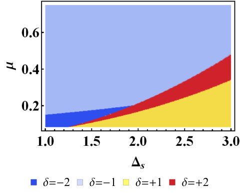
In the main text we have proposed to obtain a Fermi momentum mismatch between pσ0indp_{\sigma_{0}}^{\mathrm{ind}} and pFp_{F} by fixing the chemical potential of the substrate while tuning the chemical potential of the NW, however this can be achieved also if the NW and the substrate have the same chemical potential but different band structures (e.g. different masses), and the difference between the Fermi momenta is achieved by tuning the common chemical potential; this is easier from an experimental perspective. An example of a corresponding phase diagram is plotted in Fig. A2, note that indeed all the four combinations of topological phases are recovered.
Refer to caption
Figure A2: (Color online) The phase diagram of a 1D metallic NW deposited on top of a 2D SC substrate. We plot the value of the topological index δ\delta defined in Eq. (9) of the main text as a function of Δs\Delta_{s}, and of the chemical potential μ\mu, which is taken to be the same for the NW and the substrate. We note that all the four possible phases corresponding to δ=±1,±2\delta=\pm 1,\pm 2 can form due to the Fermi momenta mismatch occurring because of different masses of quasiparticles in the SC and the NW. We have set M=1.5,m=9,ϰ=2.5M=1.5,m=9,\varkappa=2.5, and ttun=0.5t_{\mathrm{tun}}=0.5.

Appendix B Non-TRS pp-wave

As we have already discussed in the main text, not only time-reversal-symmetric (TRS) s+ps+p–mixtures in the substrate may induce Majorana pairs at the ends of a proximitized NW. Below we consider a metallic nanowire on top of a substrate with a TRS-breaking s+ps+p–wave pairing described by the following Hamiltonian:

ℋTB=∑𝒓∈S​C,σ−μSCΨ𝒓​σ†Ψ𝒓​σ+σΔsΨ𝒓​σΨ𝒓,−σ−t∑𝒓∈S​C,σ(Ψ𝒓​σ†Ψ𝒓+𝒙,σ+Ψ𝒓​σ†Ψ𝒓+𝒚,σ)\displaystyle\mathcal{H}_{\mathrm{TB}}=\sum\limits_{\bm{r}\in SC,\sigma}-\mu_{\mathrm{SC}}\Psi^{\dagger}_{\bm{r}\sigma}\Psi_{\bm{r}\sigma}+\sigma\Delta_{s}\Psi_{\bm{r}\sigma}\Psi_{\bm{r},-\sigma}-t\sum\limits_{\bm{r}\in SC,\sigma}\left(\Psi^{\dagger}_{\bm{r}\sigma}\Psi_{\bm{r}+\bm{x},\sigma}+\Psi^{\dagger}_{\bm{r}\sigma}\Psi_{\bm{r}+\bm{y},\sigma}\right)\phantom{aaaaaaaaaaaaaaaaaaaaaaaaa}
−Δt∑𝒓∈S​C,σ(iΨ𝒓​σΨ𝒓+𝒙,−σ+Ψ𝒓​σΨ𝒓+𝒚,−σ)+∑x∈N​W,σ−μNWcx​σ†cx​σ−tcx​σ†cx+1,σ+ttun∑x∈N​W,σΨx,y=0,σ†cx,σ+H.c.\displaystyle-\Delta_{t}\negthickspace\sum\limits_{\bm{r}\in SC,\sigma}\left(i\Psi_{\bm{r}\sigma}\Psi_{\bm{r}+\bm{x},-\sigma}+\Psi_{\bm{r}\sigma}\Psi_{\bm{r}+\bm{y},-\sigma}\right)+\negthickspace\sum\limits_{x\in NW,\sigma}\negthickspace-\mu_{\mathrm{NW}}c^{\dagger}_{x\sigma}c_{x\sigma}-tc^{\dagger}_{x\sigma}c_{x+1,\sigma}+t_{\mathrm{tun}}\negthickspace\sum\limits_{x\in NW,\sigma}\Psi^{\dagger}_{x,y=0,\sigma}c_{x,\sigma}+\mathrm{H.c.}\phantom{aaa} (1)

We demonstrate in Fig. A3 that even when the time reversal symmetry is broken in the substrate in the presence of chiral pp-wave pairing, Majorana pairs still form at the ends of the wire, and a phase diagram similar to that presented in Fig. 4 of the main text can be constructed. For a non-TRS pp-wave SC these pairs cannot anymore be referred to as Kramers pairs, since it is no longer the TRS that protects them. However, they are protected by a different symmetry denoted ’magnetic mirror symmetry’ (a weaker crystalline symmetry). For details we refer the reader to Refs. [40, 41, 42].

Refer to caption
Figure A3: The phase diagram of a 1D metallic NW deposited on top of a 2D SC substrate with a mixed ss-wave and TRS-breaking pp-wave pairing. Axes and color codes are the same as in Fig. 5. The black dashed line at Δs∼0.86​t\Delta_{s}\sim 0.86t marks the bulk topological phase transition. We set μSC=3,Δt=0.5\mu_{\mathrm{SC}}=3,\Delta_{t}=0.5 and ttun=2t_{\mathrm{tun}}=2.

Appendix C Derivation of the effective Hamiltonian for the nanowire obtained by integrating out the s+ps+p-wave substrate

C.1 Model

We consider a 1D nanowire (NW) with Rashba spin-orbit coupling on top of an s+ps+p-wave 2D superconductor (SC). Writing the modified Bogoliubov-de Gennes Hamiltonian for the SC in the Nambu basis {Ψ𝒑↑,Ψ𝒑↓,Ψ−𝒑↓†,−Ψ−𝒑↑†}T\left\{\Psi_{\bm{p}\uparrow},\Psi_{\bm{p}\downarrow},\Psi^{\dagger}_{-\bm{p}\downarrow},-\Psi^{\dagger}_{-\bm{p}\uparrow}\right\}^{\mathrm{T}} we get:

ℋSC=(ξp0Δsi​ϰ​p−0ξp−i​ϰ​p+ΔsΔsi​ϰ​p−−ξp0−i​ϰ​p+Δs0−ξp),ξp=p22​M−pF22​M\displaystyle\mathcal{H}_{\mathrm{SC}}=\begin{pmatrix}\xi_{p}&0&\Delta_{s}&i\varkappa p_{-}\\ 0&\xi_{p}&-i\varkappa p_{+}&\Delta_{s}\\ \Delta_{s}&i\varkappa p_{-}&-\xi_{p}&0\\ -i\varkappa p_{+}&\Delta_{s}&0&-\xi_{p}\end{pmatrix},\quad\xi_{p}=\frac{p^{2}}{2M}-\frac{p_{F}^{2}}{2M}

where pFp_{F} is the Fermi momentum, p±=px±i​pyp_{\pm}=p_{x}\pm ip_{y}, Ψ𝒑​σ\Psi_{\bm{p}\sigma} creates an electron with momentum 𝒑\bm{p} and spin σ=↑,↓\sigma=\uparrow,\downarrow. The singlet order parameter is denoted Δs\Delta_{s}, whereas the triplet pairing is denoted ϰ\varkappa. We write the Hamiltonian of the NW in a similar Nambu basis {cpx↑,cpx↓,c−px↓†,−c−px↑†}T\left\{c_{p_{x}\uparrow},c_{p_{x}\downarrow},c^{\dagger}_{-p_{x}\downarrow},-c^{\dagger}_{-p_{x}\uparrow}\right\}^{\mathrm{T}}:

ℋNW=(ηpx0000ηpx0000−ηpx0000−ηpx),ηpx=px22​m−μ\displaystyle\mathcal{H}_{\mathrm{NW}}=\begin{pmatrix}\eta_{p_{x}}&0&0&0\\ 0&\eta_{p_{x}}&0&0\\ 0&0&-\eta_{p_{x}}&0\\ 0&0&0&-\eta_{p_{x}}\end{pmatrix},\quad\eta_{p_{x}}=\frac{p_{x}^{2}}{2m}-\mu

where μ\mu is the chemical potential. We assume that tunnelling between the NW and the SC is allowed, and that the momentum along xx axis is conserved. The corresponding Hamiltonian is given by

ℋT=ttun​∑σ∫d​𝒑(2​π)2​[Ψ𝒑​σ†​cpx​σ+cpx​σ†​Ψ𝒑​σ]\displaystyle\mathcal{H}_{\mathrm{T}}=t_{\mathrm{tun}}\sum\limits_{\sigma}\int\frac{d\bm{p}}{(2\pi)^{2}}\left[\Psi^{\dagger}_{\bm{p}\sigma}c_{p_{x}\sigma}+c^{\dagger}_{p_{x}\sigma}\Psi_{\bm{p}\sigma}\right]

In what follows we study how the interplay between different types of pairing in the SC affects the induced superconductivity in the NW.

C.2 Path integral approach

We start by writing the partition function in terms of the path integral:

𝒵=∫𝒟​cpx†​𝒟​cpx​∫𝒟​Ψ𝒑†​𝒟​Ψ𝒑​ei⁡(𝒮NW0+𝒮SC0+𝒮T),\displaystyle\mathcal{Z}=\int\mathcal{D}c^{\dagger}_{p_{x}}\mathcal{D}c_{p_{x}}\int\mathcal{D}\Psi^{\dagger}_{\bm{p}}\mathcal{D}\Psi_{\bm{p}}\,e^{i\left(\mathcal{S}_{\mathrm{NW}}^{0}+\mathcal{S}_{\mathrm{SC}}^{0}+\mathcal{S}_{\mathrm{T}}\right)}, (2)

where 𝒮NW0,𝒮SC0\mathcal{S}_{\mathrm{NW}}^{0},\mathcal{S}_{\mathrm{SC}}^{0} and 𝒮T\mathcal{S}_{\mathrm{T}} are the actions for the NW, SC and respectively for the NW-SC tunneling:

𝒮SC0\displaystyle\mathcal{S}_{\mathrm{SC}}^{0} =12​∫d​𝒑(2​π)2​d​ω2​π​Ψ𝒑†​[GSC0]−1​Ψ𝒑\displaystyle=\frac{1}{2}\int\frac{d\bm{p}}{(2\pi)^{2}}\frac{d\omega}{2\pi}\Psi_{\bm{p}}^{\dagger}\left[G_{\mathrm{SC}}^{0}\right]^{-1}\Psi_{\bm{p}}
𝒮NW0\displaystyle\mathcal{S}_{\mathrm{NW}}^{0} =12​∫d​px2​π​d​ω2​π​cpx†​[GNW0]−1​cpx\displaystyle=\frac{1}{2}\int\frac{dp_{x}}{2\pi}\frac{d\omega}{2\pi}c_{p_{x}}^{\dagger}\left[G_{\mathrm{NW}}^{0}\right]^{-1}c_{p_{x}}
𝒮T\displaystyle\mathcal{S}_{\mathrm{T}} =12​∫d​𝒑(2​π)2​d​ω2​π​[Ψ𝒑†​ℋT​cpx+cpx†​ℋT†​Ψ𝒑].\displaystyle=\frac{1}{2}\int\frac{d\bm{p}}{(2\pi)^{2}}\frac{d\omega}{2\pi}\left[\Psi_{\bm{p}}^{\dagger}\mathcal{H}_{\mathrm{T}}c_{p_{x}}+c_{p_{x}}^{\dagger}\mathcal{H}_{\mathrm{T}}^{\dagger}\Psi_{\bm{p}}\right].

We use a notation similar to the previous subsection, however here we keep in mind that cpx≡(cpx↑,cpx↓,c−px↓†,−c−px↑†)Tc_{p_{x}}\equiv\left(c_{p_{x}\uparrow},c_{p_{x}\downarrow},c^{\dagger}_{-p_{x}\downarrow},-c^{\dagger}_{-p_{x}\uparrow}\right)^{\mathrm{T}} and Ψ𝒑≡(Ψ𝒑↑,Ψ𝒑↓,Ψ−𝒑↓†,−Ψ−𝒑↑†)T\Psi_{\bm{p}}\equiv\left(\Psi_{\bm{p}\uparrow},\Psi_{\bm{p}\downarrow},\Psi^{\dagger}_{-\bm{p}\downarrow},-\Psi^{\dagger}_{-\bm{p}\uparrow}\right)^{\mathrm{T}}. The bare Green’s functions in energy-momentum space can be written as

GSC0​(ω,𝒑)=[ω+i​0−ℋSC​(𝒑)]−1,GNW0​(ω,px)=[ω+i​0−ℋNW​(px)]−1.G_{\mathrm{SC}}^{0}(\omega,\bm{p})=\left[\omega+i0-\mathcal{H}_{\mathrm{SC}}(\bm{p})\right]^{-1},\quad G_{\mathrm{NW}}^{0}(\omega,p_{x})=\left[\omega+i0-\mathcal{H}_{\mathrm{NW}}(p_{x})\right]^{-1}.

Hereinafter we integrate out the superconducting degrees of freedom and we obtain an effective action for the NW, as well as its effective Green’s function.

First, we rewrite the path integral in Eq. (2) as

𝒵=∫𝒟​cpx†​𝒟​cpx​ei​𝒮NW0​∫𝒟​Ψ𝒑†​𝒟​Ψ𝒑​ei⁡(𝒮SC0+𝒮T),\displaystyle\mathcal{Z}=\int\mathcal{D}c^{\dagger}_{p_{x}}\mathcal{D}c_{p_{x}}e^{i\mathcal{S}_{\mathrm{NW}}^{0}}\int\mathcal{D}\Psi^{\dagger}_{\bm{p}}\mathcal{D}\Psi_{\bm{p}}\,e^{i\left(\mathcal{S}_{\mathrm{SC}}^{0}+\mathcal{S}_{\mathrm{T}}\right)},

and then we perform the inner integration over the Grassmann variables Ψ𝒑†\Psi_{\bm{p}}^{\dagger} and Ψ𝒑\Psi_{\bm{p}}:

∫𝒟​Ψ𝒑†​𝒟​Ψ𝒑​ei⁡(𝒮SC+𝒮T)≡∫𝒟​Ψ𝒑†​𝒟​Ψ𝒑​exp⁡{12​∫d​𝒑(2​π)2​d​ω2​π​Ψ𝒑†​[GSC0]−1​Ψ𝒑+[Ψ𝒑†​ℋT​cpx+cpx†​ℋT†​Ψ𝒑]}\displaystyle\int\negthickspace\mathcal{D}\Psi^{\dagger}_{\bm{p}}\mathcal{D}\Psi_{\bm{p}}\,e^{i\left(\mathcal{S}_{\mathrm{SC}}+\mathcal{S}_{\mathrm{T}}\right)}\equiv\int\negthickspace\mathcal{D}\Psi^{\dagger}_{\bm{p}}\mathcal{D}\Psi_{\bm{p}}\,\exp\left\{\frac{1}{2}\int\negthickspace\frac{d\bm{p}}{(2\pi)^{2}}\frac{d\omega}{2\pi}\Psi_{\bm{p}}^{\dagger}\left[G_{\mathrm{SC}}^{0}\right]^{-1}\Psi_{\bm{p}}+\left[\Psi_{\bm{p}}^{\dagger}\mathcal{H}_{\mathrm{T}}c_{p_{x}}+c_{p_{x}}^{\dagger}\mathcal{H}_{\mathrm{T}}^{\dagger}\Psi_{\bm{p}}\right]\right\}

It is known that for a given complex-valued matrix AA and Grassmann vectors ζ\zeta and ξ†\xi^{\dagger} the integral

∫𝒟​η†​𝒟​η​exp⁡[η†​A​η+η†​ζ+ξ†​η]=detA⋅exp⁡[−ξ†​A−1​ζ].\int\negthickspace\mathcal{D}\eta^{\dagger}\mathcal{D}\eta\exp\left[\eta^{\dagger}A\eta+\eta^{\dagger}\zeta+\xi^{\dagger}\eta\right]=\det A\,\cdot\exp\left[-\xi^{\dagger}A^{-1}\zeta\right].

To obtain a similar expression we denote A≡i2​[GSC0]−1A\equiv\frac{i}{2}\left[G_{\mathrm{SC}}^{0}\right]^{-1} and ζ=i2​ℋT​cpnx,ξ†=i2​cpnx†​ℋT†\zeta=\frac{i}{2}\mathcal{H}_{\mathrm{T}}c_{p_{n_{x}}},\xi^{\dagger}=\frac{i}{2}c_{p_{n_{x}}}^{\dagger}\mathcal{H}_{\mathrm{T}}^{\dagger}, and we get:

⋆\displaystyle\star =det[i2​(GSC0)−1]⋅exp⁡{(−i2​cpnx†​ℋT†)​(2i​GSC0)​(i2​ℋT​cpnx)}=\displaystyle=\det\left[\frac{i}{2}\left(G_{\mathrm{SC}}^{0}\right)^{-1}\right]\cdot\exp\left\{\left(-\frac{i}{2}c_{p_{n_{x}}}^{\dagger}\mathcal{H}_{\mathrm{T}}^{\dagger}\right)\left(\frac{2}{i}G_{\mathrm{SC}}^{0}\right)\left(\frac{i}{2}\mathcal{H}_{\mathrm{T}}c_{p_{n_{x}}}\right)\right\}=
=det[i2​(GSC0)−1]⋅exp⁡{−i2​cpnx†​ℋT†​GSC0​ℋT​cpnx}\displaystyle=\det\left[\frac{i}{2}\left(G_{\mathrm{SC}}^{0}\right)^{-1}\right]\cdot\exp\left\{-\frac{i}{2}c_{p_{n_{x}}}^{\dagger}\mathcal{H}_{\mathrm{T}}^{\dagger}G_{\mathrm{SC}}^{0}\mathcal{H}_{\mathrm{T}}c_{p_{n_{x}}}\right\}

Before inserting this expression back into the partition function, we employ the fact that the functional determinant is absorbed into the measure. Thus we have

𝒵∝∫𝒟cpx†𝒟cpxei​𝒮NW0⋅exp{i∫d​px2​πd​ω2​πcpnx†[−12∫d​py2​πℋT†GSC0ℋT]cpnx}\displaystyle\mathcal{Z}\propto\int\mathcal{D}c^{\dagger}_{p_{x}}\mathcal{D}c_{p_{x}}e^{i\mathcal{S}_{\mathrm{NW}}^{0}}\cdot\exp\left\{i\int\negthickspace\frac{dp_{x}}{2\pi}\frac{d\omega}{2\pi}c_{p_{n_{x}}}^{\dagger}\left[-\frac{1}{2}\int\negthickspace\frac{dp_{y}}{2\pi}\mathcal{H}_{\mathrm{T}}^{\dagger}G_{\mathrm{SC}}^{0}\mathcal{H}_{\mathrm{T}}\right]c_{p_{n_{x}}}\right\}

Finally, the effective action and Green’s function for the NW can be written as

𝒮NW=𝒮NW0+∫d​px2​πd​ω2​πcpnx†[−12∫d​py2​πℋT†GSC0ℋT]cpnx\displaystyle\mathcal{S}_{\mathrm{NW}}=\mathcal{S}_{\mathrm{NW}}^{0}+\int\negthickspace\frac{dp_{x}}{2\pi}\frac{d\omega}{2\pi}c_{p_{n_{x}}}^{\dagger}\left[-\frac{1}{2}\int\negthickspace\frac{dp_{y}}{2\pi}\mathcal{H}_{\mathrm{T}}^{\dagger}G_{\mathrm{SC}}^{0}\mathcal{H}_{\mathrm{T}}\right]c_{p_{n_{x}}}

and

GNW−1=(GNW0)−1−∫d​py2​π​ℋT†​GSC0​ℋT\displaystyle G_{\mathrm{NW}}^{-1}=\left(G^{0}_{\mathrm{NW}}\right)^{-1}-\int\negthickspace\frac{dp_{y}}{2\pi}\mathcal{H}_{\mathrm{T}}^{\dagger}G_{\mathrm{SC}}^{0}\mathcal{H}_{\mathrm{T}}

C.3 Effective Green’s function for the nanowire

As we have just demonstrated above, within the path integral formalism, integrating out the superconducting degrees of freedom is equivalent to integrating the retarded Green’s function of the superconductor over pyp_{y} – the momentum along the direction perpendicular to the axis of the NW. Therefore, we can write the ”perturbed” retarded Green’s function of the NW in the following form:

GNW​(ω,px)=[ω+i​0−ℋNW​(px)−ttun2​∑pyGSC0​(ω,px,py)]−1,\displaystyle G_{\mathrm{NW}}(\omega,p_{x})=\left[\omega+i0-\mathcal{H}_{\mathrm{NW}}(p_{x})-t_{\mathrm{tun}}^{2}\sum\limits_{p_{y}}G_{\mathrm{SC}}^{0}(\omega,p_{x},p_{y})\right]^{-1},

where we defined

GSC0​(ω,px,py)=[ω+i​0−ℋSC​(px,py)]−1.\displaystyle G_{\mathrm{SC}}^{0}(\omega,p_{x},p_{y})=\left[\omega+i0-\mathcal{H}_{\mathrm{SC}}(p_{x},p_{y})\right]^{-1}.

We start by rewriting the retarded Green’s function of the SC as GSC0=12∑σ=±G0σG_{\mathrm{SC}}^{0}=\frac{1}{2}\sum\limits_{\sigma=\pm}G_{0}^{\sigma}, where

G0σ(ω,𝒑)=−1ξp2+(Δs+σ​ϰ​p)2−ω2(1i​σ​e−i​ϕ𝒑−i​σ​ei​ϕ𝒑1)⊗(ω+ξpΔs+σ​ϰ​pΔs+σ​ϰ​pω−ξp),\displaystyle G_{0}^{\sigma}(\omega,\bm{p})=-\frac{1}{\xi_{p}^{2}+(\Delta_{s}+\sigma\varkappa p)^{2}-\omega^{2}}\begin{pmatrix}1&i\sigma e^{-i\phi_{\bm{p}}}\\ -i\sigma e^{i\phi_{\bm{p}}}&1\end{pmatrix}\otimes\begin{pmatrix}\omega+\xi_{p}&\Delta_{s}+\sigma\varkappa p\\ \Delta_{s}+\sigma\varkappa p&\omega-\xi_{p}\end{pmatrix},

with p≡py2+px2p\equiv\sqrt{p_{y}^{2}+p_{x}^{2}} and ei​s​ϕ𝒑≡px+i​s​pype^{is\phi_{\bm{p}}}\equiv\frac{p_{x}+isp_{y}}{p} (s=±1s=\pm 1). To integrate this function over pyp_{y} we linearize ξp\xi_{p} around the Fermi energy ξp=vF​(p−pF)\xi_{p}=v_{F}(p-p_{F}), where vF≡pF/mv_{F}\equiv p_{F}/m is the Fermi velocity. There are four different integrations to perform, namely

X0σ\displaystyle X_{0}^{\sigma} =−∫d​py2​π1ξp2+(Δs+σ​ϰ​p)2−ω2\displaystyle=-\int\frac{dp_{y}}{2\pi}\frac{1}{\xi_{p}^{2}+(\Delta_{s}+\sigma\varkappa p)^{2}-\omega^{2}}
X1σ\displaystyle X_{1}^{\sigma} =−∫d​py2​πξpξp2+(Δs+σ​ϰ​p)2−ω2\displaystyle=-\int\frac{dp_{y}}{2\pi}\frac{\xi_{p}}{\xi_{p}^{2}+(\Delta_{s}+\sigma\varkappa p)^{2}-\omega^{2}}
X2σ\displaystyle X_{2}^{\sigma} =−∫d​py2​πei​s​ϕ𝒑ξp2+(Δs+σ​ϰ​p)2−ω2\displaystyle=-\int\frac{dp_{y}}{2\pi}\frac{e^{is\phi_{\bm{p}}}}{\xi_{p}^{2}+(\Delta_{s}+\sigma\varkappa p)^{2}-\omega^{2}}
X3σ\displaystyle X_{3}^{\sigma} =−∫d​py2​πξp​ei​s​ϕ𝒑ξp2+(Δs+σ​ϰ​p)2−ω2\displaystyle=-\int\frac{dp_{y}}{2\pi}\frac{\xi_{p}\,e^{is\phi_{\bm{p}}}}{\xi_{p}^{2}+(\Delta_{s}+\sigma\varkappa p)^{2}-\omega^{2}}

We start by considering the case of px≠0p_{x}\neq 0 and we modify the integrand

−∫d​py2​π(∙)ξp2+(Δs+σ​ϰ​p)2−ω2=|py=pxshq|=−1vF2+ϰ21|px|∫d​q2​πch⁡q(ch⁡q+Aσ)2+Ωσ2(∙),-\int\frac{dp_{y}}{2\pi}\frac{(\bullet)}{\xi_{p}^{2}+(\Delta_{s}+\sigma\varkappa p)^{2}-\omega^{2}}=\Bigg|p_{y}=p_{x}\sh q\Bigg|=-\frac{1}{v_{F}^{2}+\varkappa^{2}}\frac{1}{|p_{x}|}\int\frac{dq}{2\pi}\frac{\ch q}{(\ch q+A_{\sigma})^{2}+\Omega_{\sigma}^{2}}(\bullet),

where

Aσ≡σ​ϰ​Δs−pF​vF2(vF2+ϰ2)​|px|,Ωσ≡(Δeffσ)2−ω2|px|​vF2+ϰ2,Δeffσ≡|Δs+σ​ϰ​pF|1+ϰ2/vF2A_{\sigma}\equiv\frac{\sigma\varkappa\Delta_{s}-p_{F}v_{F}^{2}}{(v_{F}^{2}+\varkappa^{2})|p_{x}|},\quad\Omega_{\sigma}\equiv\frac{\sqrt{\left(\Delta_{\mathrm{eff}}^{\sigma}\right)^{2}-\omega^{2}}}{|p_{x}|\sqrt{v_{F}^{2}+\varkappa^{2}}},\quad\Delta_{\mathrm{eff}}^{\sigma}\equiv\frac{\left|\Delta_{s}+\sigma\varkappa p_{F}\right|}{\sqrt{1+\varkappa^{2}/v_{F}^{2}}}
(∙)=1,(∙)=vF​(|px|​ch⁡q−pF),(∙)=px|px|​1+i​s​sh⁡qch⁡q,(∙)=vF​(|px|​ch⁡q−pF)​px|px|​1+i​s​sh⁡qch⁡q(\bullet)=1,\quad(\bullet)=v_{F}(|p_{x}|\ch q-p_{F}),\quad(\bullet)=\frac{p_{x}}{|p_{x}|}\frac{1+is\sh q}{\ch q},\quad(\bullet)=v_{F}(|p_{x}|\ch q-p_{F})\frac{p_{x}}{|p_{x}|}\frac{1+is\sh q}{\ch q}

for X0,X1,X2X_{0},X_{1},X_{2} and X3X_{3} correspondingly. For the sake of simplicity, in what follows we consider only in-gap energies, i.e. |ω|<Δeffσ|\omega|<\Delta_{\mathrm{eff}}^{\sigma}, and we compute the zeroth integral

X0σ=1vF2+ϰ2​1|px|​2π​Ωσ​Im⁡[Aσ+i​Ωσ1−(Aσ+i​Ωσ)2​arctg⁡−1+Aσ+i​Ωσ1−(Aσ+i​Ωσ)2].\displaystyle X_{0}^{\sigma}=\frac{1}{v_{F}^{2}+\varkappa^{2}}\frac{1}{|p_{x}|}\frac{2}{\pi\Omega_{\sigma}}\im\left[\frac{A_{\sigma}+i\Omega_{\sigma}}{\sqrt{1-(A_{\sigma}+i\Omega_{\sigma})^{2}}}\arctg\frac{-1+A_{\sigma}+i\Omega_{\sigma}}{\sqrt{1-(A_{\sigma}+i\Omega_{\sigma})^{2}}}\right].

We proceed with the 1st integral and we note that

X1σ=−pF​vF​X0σ−vFvF2+ϰ2​∫d​q2​π​ch2⁡q(ch⁡q+Aσ)2+Ωσ2,X_{1}^{\sigma}=-p_{F}v_{F}X_{0}^{\sigma}-\frac{v_{F}}{v_{F}^{2}+\varkappa^{2}}\int\frac{dq}{2\pi}\frac{\ch^{2}q}{(\ch q+A_{\sigma})^{2}+\Omega_{\sigma}^{2}},

where the last integral has a logarithmic UV divergence. To calculate it we introduce a cutoff in the following way

∫d​q2​π​ch2⁡q(ch⁡q+Aσ)2+Ωσ2=limΛ→+∞∫d​q2​π​ch2⁡q(ch⁡q+Aσ)2+Ωσ2⋅Λ2(ch⁡q+Aσ)2+Λ2.\int\frac{dq}{2\pi}\frac{\ch^{2}q}{(\ch q+A_{\sigma})^{2}+\Omega_{\sigma}^{2}}=\lim\limits_{\Lambda\to+\infty}\int\frac{dq}{2\pi}\frac{\ch^{2}q}{(\ch q+A_{\sigma})^{2}+\Omega_{\sigma}^{2}}\cdot\frac{\Lambda^{2}}{(\ch q+A_{\sigma})^{2}+\Lambda^{2}}.

The integral can be done straightforwardly, and we obtain

∫d​q2​π​ch2⁡q(ch⁡q+Aσ)2+Ωσ2⋅Λ2(ch⁡q+Aσ)2+Λ2=\displaystyle\int\frac{dq}{2\pi}\frac{\ch^{2}q}{(\ch q+A_{\sigma})^{2}+\Omega_{\sigma}^{2}}\cdot\frac{\Lambda^{2}}{(\ch q+A_{\sigma})^{2}+\Lambda^{2}}=\phantom{aaaaaaaaaaaaaaaaaaaaaaaaaaaaaaaaaaaaaaaa}
−2πΛ2Λ2−Ωσ2{1ΛIm[(Aσ+i​Λ)21−(Aσ+i​Λ)2arctg−1+Aσ+i​Λ1−(Aσ+i​Λ)2]−\displaystyle-\frac{2}{\pi}\frac{\Lambda^{2}}{\Lambda^{2}-\Omega_{\sigma}^{2}}\left\{\frac{1}{\Lambda}\im\left[\frac{(A_{\sigma}+i\Lambda)^{2}}{\sqrt{1-(A_{\sigma}+i\Lambda)^{2}}}\arctg\frac{-1+A_{\sigma}+i\Lambda}{\sqrt{1-(A_{\sigma}+i\Lambda)^{2}}}\right]-\right.\phantom{aaaaaaaaaaaaaaa}
−1ΩσIm[(Aσ+i​Ωσ)21−(Aσ+i​Ωσ)2arctg−1+Aσ+i​Ωσ1−(Aσ+i​Ωσ)2]}=⋆\displaystyle\left.-\frac{1}{\Omega_{\sigma}}\im\left[\frac{(A_{\sigma}+i\Omega_{\sigma})^{2}}{\sqrt{1-(A_{\sigma}+i\Omega_{\sigma})^{2}}}\arctg\frac{-1+A_{\sigma}+i\Omega_{\sigma}}{\sqrt{1-(A_{\sigma}+i\Omega_{\sigma})^{2}}}\right]\right\}=\star

We expand the expression above keeping only the leading terms in 1/Λ1/\Lambda:

⋆=2π​Ωσ​Im⁡[(Aσ+i​Ωσ)21−(Aσ+i​Ωσ)2​arctg⁡−1+Aσ+i​Ωσ1−(Aσ+i​Ωσ)2]+1π​ln⁡2​Λ+O⁡(1Λ)\displaystyle\star=\frac{2}{\pi\Omega_{\sigma}}\im\left[\frac{(A_{\sigma}+i\Omega_{\sigma})^{2}}{\sqrt{1-(A_{\sigma}+i\Omega_{\sigma})^{2}}}\arctg\frac{-1+A_{\sigma}+i\Omega_{\sigma}}{\sqrt{1-(A_{\sigma}+i\Omega_{\sigma})^{2}}}\right]+\frac{1}{\pi}\logn 2\Lambda+O\left(\frac{1}{\Lambda}\right)

Along similar lines we compute the second integral

X2σ=−1vF2+ϰ2​1px​2π​Ωσ​Im⁡[11−(Aσ+i​Ωσ)2​arctg⁡−1+Aσ+i​Ωσ1−(Aσ+i​Ωσ)2].\displaystyle X_{2}^{\sigma}=-\frac{1}{v_{F}^{2}+\varkappa^{2}}\frac{1}{p_{x}}\frac{2}{\pi\Omega_{\sigma}}\im\left[\frac{1}{\sqrt{1-(A_{\sigma}+i\Omega_{\sigma})^{2}}}\arctg\frac{-1+A_{\sigma}+i\Omega_{\sigma}}{\sqrt{1-(A_{\sigma}+i\Omega_{\sigma})^{2}}}\right].

Note, that there is no dependence on the sign of ss, even though it is present in the definition. The third integral can be expressed in terms of the zeroth and the second ones:

X3σ=vF​(px​X0σ−pF​X2σ)\displaystyle X_{3}^{\sigma}=v_{F}(p_{x}X_{0}^{\sigma}-p_{F}X_{2}^{\sigma})

To obtain the integrals computed above in the limit of px=0p_{x}=0, we take the limit limpx→0\lim\limits_{p_{x}\to 0} (it is not difficult to see that those limits exist). Finally, we write the retarded Green’s function integrated over pyp_{y} in terms of all the integrals computed above:

∫d​py2​π​G0σ​(ω,𝒑)=\displaystyle\int\frac{dp_{y}}{2\pi}G_{0}^{\sigma}(\omega,\bm{p})=
=(ω​X0σ+X1σi​σ​(ω​X2σ+X3σ)Δσ​X0σ+σ​ϰ~​X1σi​σ​(Δσ​X2σ+σ​ϰ~​X3σ)−i​σ​(ω​X2σ+X3σ)ω​X0σ+X1σ−i​σ​(Δσ​X2σ+σ​ϰ~​X3σ)Δσ​X0σ+σ​ϰ~​X1σΔσ​X0σ+σ​ϰ~​X1σi​σ​(Δσ​X2σ+σ​ϰ~​X3σ)ω​X0σ−X1σi​σ​(ω​X2σ−X3σ)−i​σ​(Δσ​X2σ+σ​ϰ~​X3σ)Δσ​X0σ+σ​ϰ~​X1σ−i​σ​(ω​X2σ−X3σ)ω​X0σ−X1σ)≡\displaystyle=\begin{pmatrix}\omega X_{0}^{\sigma}+X_{1}^{\sigma}&i\sigma(\omega X_{2}^{\sigma}+X_{3}^{\sigma})&\Delta_{\sigma}X_{0}^{\sigma}+\sigma\tilde{\varkappa}X_{1}^{\sigma}&i\sigma\left(\Delta_{\sigma}X_{2}^{\sigma}+\sigma\tilde{\varkappa}X_{3}^{\sigma}\right)\\ -i\sigma(\omega X_{2}^{\sigma}+X_{3}^{\sigma})&\omega X_{0}^{\sigma}+X_{1}^{\sigma}&-i\sigma\left(\Delta_{\sigma}X_{2}^{\sigma}+\sigma\tilde{\varkappa}X_{3}^{\sigma}\right)&\Delta_{\sigma}X_{0}^{\sigma}+\sigma\tilde{\varkappa}X_{1}^{\sigma}\\ \Delta_{\sigma}X_{0}^{\sigma}+\sigma\tilde{\varkappa}X_{1}^{\sigma}&i\sigma\left(\Delta_{\sigma}X_{2}^{\sigma}+\sigma\tilde{\varkappa}X_{3}^{\sigma}\right)&\omega X_{0}^{\sigma}-X_{1}^{\sigma}&i\sigma(\omega X_{2}^{\sigma}-X_{3}^{\sigma})\\ -i\sigma\left(\Delta_{\sigma}X_{2}^{\sigma}+\sigma\tilde{\varkappa}X_{3}^{\sigma}\right)&\Delta_{\sigma}X_{0}^{\sigma}+\sigma\tilde{\varkappa}X_{1}^{\sigma}&-i\sigma(\omega X_{2}^{\sigma}-X_{3}^{\sigma})&\omega X_{0}^{\sigma}-X_{1}^{\sigma}\end{pmatrix}\equiv
≡X0σ​σ0⊗(ω​τ0+Δσ​τx)+X1σ​σ0⊗(τz+σ​ϰ~​τx)−σ​X2σ​σy⊗(ω​τ0+Δσ​τx)−X3σ​σy⊗(σ​τz+ϰ~​τx).\displaystyle\equiv X_{0}^{\sigma}\sigma_{0}\otimes(\omega\tau_{0}+\Delta_{\sigma}\tau_{x})+X_{1}^{\sigma}\sigma_{0}\otimes(\tau_{z}+\sigma\tilde{\varkappa}\tau_{x})-\sigma X_{2}^{\sigma}\sigma_{y}\otimes(\omega\tau_{0}+\Delta_{\sigma}\tau_{x})-X_{3}^{\sigma}\sigma_{y}\otimes(\sigma\tau_{z}+\tilde{\varkappa}\tau_{x}). (3)

where we denoted ϰ~=ϰ/vF\tilde{\varkappa}=\varkappa/v_{F} and Δσ≡Δs+σ​ϰ​pF\Delta_{\sigma}\equiv\Delta_{s}+\sigma\varkappa p_{F} (not to confuse with Δeffσ\Delta^{\sigma}_{\mathrm{eff}}).

Bringing together all the expressions calculated above we have:

X0σ=1vF2+ϰ2​2π​Ωσ~​Im⁡[Aσ~+i​Ωσ~px2−(Aσ~+i​Ωσ~)2​arctg⁡−|px|+Aσ~+i​Ωσ~px2−(Aσ~+i​Ωσ~)2]\displaystyle X_{0}^{\sigma}=\frac{1}{v_{F}^{2}+\varkappa^{2}}\frac{2}{\pi\widetilde{\Omega_{\sigma}}}\im\left[\frac{\widetilde{A_{\sigma}}+i\widetilde{\Omega_{\sigma}}}{\sqrt{p_{x}^{2}-(\widetilde{A_{\sigma}}+i\widetilde{\Omega_{\sigma}})^{2}}}\arctg\frac{-|p_{x}|+\widetilde{A_{\sigma}}+i\widetilde{\Omega_{\sigma}}}{\sqrt{p_{x}^{2}-(\widetilde{A_{\sigma}}+i\widetilde{\Omega_{\sigma}})^{2}}}\right]
X1σ=−pF​vF​X0σ−vFvF2+ϰ2​{2π​Ωσ~​Im⁡[(Aσ~+i​Ωσ~)2px2−(Aσ~+i​Ωσ~)2​arctg⁡−|px|+Aσ~+i​Ωσ~px2−(Aσ~+i​Ωσ~)2]+1π​ln⁡2​Λ}\displaystyle X_{1}^{\sigma}=-p_{F}v_{F}X_{0}^{\sigma}-\frac{v_{F}}{v_{F}^{2}+\varkappa^{2}}\left\{\frac{2}{\pi\widetilde{\Omega_{\sigma}}}\im\left[\frac{(\widetilde{A_{\sigma}}+i\widetilde{\Omega_{\sigma}})^{2}}{\sqrt{p_{x}^{2}-(\widetilde{A_{\sigma}}+i\widetilde{\Omega_{\sigma}})^{2}}}\arctg\frac{-|p_{x}|+\widetilde{A_{\sigma}}+i\widetilde{\Omega_{\sigma}}}{\sqrt{p_{x}^{2}-(\widetilde{A_{\sigma}}+i\widetilde{\Omega_{\sigma}})^{2}}}\right]\negthickspace+\frac{1}{\pi}\logn 2\Lambda\right\}
X2σ=−1vF2+ϰ22π​Ωσ~⋅px⋅Im[1px2−(Aσ~+i​Ωσ~)2arctg−|px|+Aσ~+i​Ωσ~px2−(Aσ~+i​Ωσ~)2]\displaystyle X_{2}^{\sigma}=-\frac{1}{v_{F}^{2}+\varkappa^{2}}\frac{2}{\pi\widetilde{\Omega_{\sigma}}}\cdot p_{x}\cdot\im\left[\frac{1}{\sqrt{p_{x}^{2}-(\widetilde{A_{\sigma}}+i\widetilde{\Omega_{\sigma}})^{2}}}\arctg\frac{-|p_{x}|+\widetilde{A_{\sigma}}+i\widetilde{\Omega_{\sigma}}}{\sqrt{p_{x}^{2}-(\widetilde{A_{\sigma}}+i\widetilde{\Omega_{\sigma}})^{2}}}\right]
X3σ=vF​(px​X0σ−pF​X2σ),\displaystyle X_{3}^{\sigma}=v_{F}\left(p_{x}X_{0}^{\sigma}-p_{F}X_{2}^{\sigma}\right),

where tildes mean that the corresponding functions are taken at px=1p_{x}=1, i.e. Aσ~=Aσ​(px=1)\widetilde{A_{\sigma}}=A_{\sigma}(p_{x}=1) and Ωσ~=Ωσ​(px=1)\widetilde{\Omega_{\sigma}}=\Omega_{\sigma}(p_{x}=1).

C.4 Studying the induced pairing

We now study the low-energy approximation for the NW. Following Ref. [15] we assume that its effective Hamiltonian can be found as

ℋNWeff=−[GNW​(ω=0,px)]−1,\mathcal{H}_{\mathrm{NW}}^{\mathrm{eff}}=-\left[G_{\mathrm{NW}}(\omega=0,p_{x})\right]^{-1},

where we keep all the terms up to those linear in pxp_{x}. The induced singlet pairing is given by (ℋNWeff)13\left(\mathcal{H}_{\mathrm{NW}}^{\mathrm{eff}}\right)_{13}, whereas the induced triplet pairing is defined by (ℋNWeff)14\left(\mathcal{H}_{\mathrm{NW}}^{\mathrm{eff}}\right)_{14}. It is easy to check that the corresponding symmetries are respected, i.e. the singlet pairing term is even in pxp_{x}, whereas the triplet pairing term is odd.

We substitute all the functions in Eq. (3) to obtain an effective low-energy Hamiltonian. The induced pairing terms can be found as

Δsind=ttun2π​vF​limpx→0∑σ1|Δσ|​Im⁡[Δσ−i​σ​ϰ~​|Δσ|1+ϰ~2​Aσ~+i​Ωσ~px2−(Aσ~+i​Ωσ~)2​arctg⁡−|px|+Aσ~+i​Ωσ~px2−(Aσ~+i​Ωσ~)2]\displaystyle\Delta_{s}^{\mathrm{ind}}=\frac{t_{\mathrm{tun}}^{2}}{\pi v_{F}}\lim\limits_{p_{x}\to 0}\sum\limits_{\sigma}\frac{1}{|\Delta_{\sigma}|}\im\left[\frac{\Delta_{\sigma}-i\sigma\tilde{\varkappa}|\Delta_{\sigma}|}{1+\tilde{\varkappa}^{2}}\frac{\widetilde{A_{\sigma}}+i\widetilde{\Omega_{\sigma}}}{\sqrt{p_{x}^{2}-(\widetilde{A_{\sigma}}+i\widetilde{\Omega_{\sigma}})^{2}}}\arctg\frac{-|p_{x}|+\widetilde{A_{\sigma}}+i\widetilde{\Omega_{\sigma}}}{\sqrt{p_{x}^{2}-(\widetilde{A_{\sigma}}+i\widetilde{\Omega_{\sigma}})^{2}}}\right]
ϰind=ttun2π​vF​limpx→0∑σ−σ|Δσ|​Im⁡[Δσ−i​σ​ϰ~​|Δσ|1+ϰ~2​1px2−(Aσ~+i​Ωσ~)2​arctg⁡−|px|+Aσ~+i​Ωσ~px2−(Aσ~+i​Ωσ~)2]\displaystyle\varkappa^{\mathrm{ind}}=\frac{t_{\mathrm{tun}}^{2}}{\pi v_{F}}\lim\limits_{p_{x}\to 0}\sum\limits_{\sigma}\frac{-\sigma}{|\Delta_{\sigma}|}\im\left[\frac{\Delta_{\sigma}-i\sigma\tilde{\varkappa}|\Delta_{\sigma}|}{1+\tilde{\varkappa}^{2}}\frac{1}{\sqrt{p_{x}^{2}-(\widetilde{A_{\sigma}}+i\widetilde{\Omega_{\sigma}})^{2}}}\arctg\frac{-|p_{x}|+\widetilde{A_{\sigma}}+i\widetilde{\Omega_{\sigma}}}{\sqrt{p_{x}^{2}-(\widetilde{A_{\sigma}}+i\widetilde{\Omega_{\sigma}})^{2}}}\right]
λind=ttun2π​vF​limpx→0∑σσ|Δσ|​Re⁡[|Δσ|−i​σ​ϰ~​Δσ1+ϰ~2​1px2−(Aσ~+i​Ωσ~)2​arctg⁡−|px|+Aσ~+i​Ωσ~px2−(Aσ~+i​Ωσ~)2]\displaystyle\lambda^{\mathrm{ind}}=\frac{t_{\mathrm{tun}}^{2}}{\pi v_{F}}\lim\limits_{p_{x}\to 0}\sum\limits_{\sigma}\frac{\sigma}{|\Delta_{\sigma}|}\re\left[\frac{|\Delta_{\sigma}|-i\sigma\tilde{\varkappa}\Delta_{\sigma}}{1+\tilde{\varkappa}^{2}}\frac{1}{\sqrt{p_{x}^{2}-(\widetilde{A_{\sigma}}+i\widetilde{\Omega_{\sigma}})^{2}}}\arctg\frac{-|p_{x}|+\widetilde{A_{\sigma}}+i\widetilde{\Omega_{\sigma}}}{\sqrt{p_{x}^{2}-(\widetilde{A_{\sigma}}+i\widetilde{\Omega_{\sigma}})^{2}}}\right]

Note that the functions in square brackets are not analytical at px=0p_{x}=0, and therefore we must keep the limit sign and we cannot just set px=0p_{x}=0. Numerically it means that we evaluate these functions for a very small non-zero value of pxp_{x}. We define also a renormalized chemical potential

μind=μ−ttun22​limpx→0∑σX1σ=\displaystyle\mu^{\mathrm{ind}}=\mu-\frac{t_{\mathrm{tun}}^{2}}{2}\lim\limits_{p_{x}\to 0}\sum\limits_{\sigma}X_{1}^{\sigma}=
=μ+ttun2π​vF​{ln⁡2​Λ1+ϰ~2+limpx→0∑σ1|Δσ|​Re⁡[|Δσ|−i​σ​ϰ~​Δσ1+ϰ~2​Aσ~+i​Ωσ~px2−(Aσ~+i​Ωσ~)2​arctg⁡−|px|+Aσ~+i​Ωσ~px2−(Aσ~+i​Ωσ~)2]}\displaystyle=\mu+\frac{t_{\mathrm{tun}}^{2}}{\pi v_{F}}\left\{\frac{\logn 2\Lambda}{1+\tilde{\varkappa}^{2}}+\lim\limits_{p_{x}\to 0}\sum\limits_{\sigma}\frac{1}{|\Delta_{\sigma}|}\re\left[\frac{|\Delta_{\sigma}|-i\sigma\tilde{\varkappa}\Delta_{\sigma}}{1+\tilde{\varkappa}^{2}}\frac{\widetilde{A_{\sigma}}+i\widetilde{\Omega_{\sigma}}}{\sqrt{p_{x}^{2}-(\widetilde{A_{\sigma}}+i\widetilde{\Omega_{\sigma}})^{2}}}\arctg\frac{-|p_{x}|+\widetilde{A_{\sigma}}+i\widetilde{\Omega_{\sigma}}}{\sqrt{p_{x}^{2}-(\widetilde{A_{\sigma}}+i\widetilde{\Omega_{\sigma}})^{2}}}\right]\right\}

In terms of the constants defined above we write an effective low-energy Hamiltonian for the NW:

HNWeff=(px22​m−μindi​λind​pxΔsindi​ϰind​px−i​λind​pxpx22​m−μind−i​ϰind​pxΔsindΔsindi​ϰind​px−(px22​m−μind)−i​λind​px−i​ϰind​pxΔsindi​λind​px−(px22​m−μind)),H_{\mathrm{NW}}^{\mathrm{eff}}=\begin{pmatrix}\frac{p_{x}^{2}}{2m}-\mu^{\mathrm{ind}}&i\lambda^{\mathrm{ind}}p_{x}&\Delta_{s}^{\mathrm{ind}}&i\varkappa^{\mathrm{ind}}p_{x}\\ -i\lambda^{\mathrm{ind}}p_{x}&\frac{p_{x}^{2}}{2m}-\mu^{\mathrm{ind}}&-i\varkappa^{\mathrm{ind}}p_{x}&\Delta_{s}^{\mathrm{ind}}\\ \Delta_{s}^{\mathrm{ind}}&i\varkappa^{\mathrm{ind}}p_{x}&-\left(\frac{p_{x}^{2}}{2m}-\mu^{\mathrm{ind}}\right)&-i\lambda^{\mathrm{ind}}p_{x}\\ -i\varkappa^{\mathrm{ind}}p_{x}&\Delta_{s}^{\mathrm{ind}}&i\lambda^{\mathrm{ind}}p_{x}&-\left(\frac{p_{x}^{2}}{2m}-\mu^{\mathrm{ind}}\right)\end{pmatrix}, (4)

or equivalently

HNWeff=(px22​m−μind)​σ0⊗τz−λind​px​σy⊗τz+Δsind​σ0⊗τx−ϰind​px​σy⊗τx.H_{\mathrm{NW}}^{\mathrm{eff}}=\left(\frac{p_{x}^{2}}{2m}-\mu^{\mathrm{ind}}\right)\sigma_{0}\otimes\tau_{z}-\lambda^{\mathrm{ind}}\,p_{x}\sigma_{y}\otimes\tau_{z}+\Delta_{s}^{\mathrm{ind}}\,\sigma_{0}\otimes\tau_{x}-\varkappa^{\mathrm{ind}}\,p_{x}\sigma_{y}\otimes\tau_{x}.

To find the gap for the Hamiltonian in Eq. (4) we linearize its spectrum around two different Fermi momenta emerging due to non-zero induced spin-orbit coupling value:

Δeffind=minσ⁡|Δsind−m​ϰind​(λind−σ​(λind)2+2​μind/m)|1+(ϰind)2(λind)2+2​μind/m\Delta^{\mathrm{ind}}_{\mathrm{eff}}=\min\limits_{\sigma}\frac{\left|\Delta^{\mathrm{ind}}_{s}-m\varkappa^{\mathrm{ind}}\left(\lambda^{\mathrm{ind}}-\sigma\sqrt{(\lambda^{\mathrm{ind}})^{2}+2\mu^{\mathrm{ind}}/m}\right)\right|}{\sqrt{1+\frac{(\varkappa^{\mathrm{ind}})^{2}}{(\lambda^{\mathrm{ind}})^{2}+2\mu^{\mathrm{ind}}/m}}}