True versus apparent shapes of bow shocks

Consider body-frame cartesian coordinates $(x,y,z)$, where $x$ is the symmetry axis, and spherical polar coordinates $(R,\theta,\phi)$, where $\theta$ is the polar angle and $\phi$ the azimuthal angle. Since the surface is cylindrically symmetric, it is can be specified as $R=R(\theta)$, so that cartesian coordinates on the surface are:

Suppose that the viewing direction makes an angle $i$ with the $z$ axis, so that we can define observer-frame coordinates $(x^{\prime},y^{\prime},z^{\prime})$, which are found by rotating the body-frame coordinates about the $y$ axis. The same vector, $\bm{r}$, expressed in the observer frame is then

where the rotation matrix $\textbf{{A}}_{y}(i)$ is given in Appendix B. The inclination angle $i$ is defined so that $i=$$$ when the surface is viewed perpendicular to its axis (side on) and $i=\pm$$$ when it is viewed along its axis (end on), with positive $i$ when the apex points towards the observer.

The relationship between the two frames is illustrated in Figure 5. All quantities in the observer’s frame are denoted by attaching a prime to the equivalent quantity in the body frame. There are two ways of interpreting the primed coordinates. On the one hand, the 3-vector $(x^{\prime},y^{\prime},z^{\prime})$ specifies a point in Euclidean space, $\mathds{R}^{3}$, but an alternative interpretation is to take the 2-vector $(x^{\prime},y^{\prime})$ as specifying a point in a projective space, $\mathds{P}^{2}$ (see, for example, § 15.6 of Penrose, 2004). Each “point” in $\mathds{P}^{2}$ is equivalent to a line in $\mathds{R}^{3}$, specifically: a line of sight that passes through the observer. Thus, $(x^{\prime},y^{\prime})$ gives the celestial coordinates on the plane of the sky, with $x^{\prime}$ being the projected symmetry axis of the surface. We assume that the observer is located at a very large distance, relative to the size of the bow, so that all lines of sight are effectively parallel to the $z^{\prime}$ axis, with the observer at $z^{\prime}=-\infty$. But, from the point of view of the plane of the sky, the $z^{\prime}$ coordinate is strictly irrelevant since it is a projective plane, and not a Euclidean plane. In the following, we will switch between the $\mathds{R}^{3}$ and $\mathds{P}^{2}$ interpretations as convenient, resolving ambiguity where necessary via the adjectives “Euclidean” for $\mathds{R}^{3}$ and “plane-of-sky” or “projected” for $\mathds{P}^{2}$.

We define unit vectors $\bm{\hat{n}},\bm{\hat{t}}$, such that $\bm{\hat{n}}$ is normal to the surface, while $\bm{\hat{t}}$ is tangent to the surface in a plane of constant $\phi$. For $\phi=0$ the surface lies in the $xy$ plane and it is straightforward to show (Fig. 6) that in this case the unit vectors are given by

where $\alpha$ is the slope angle, given by

and $\omega$ is a dimensionless local growth factor:

For general $\phi\neq 0$, we find $\bm{\hat{n}}$ and $\bm{\hat{t}}$ by rotating equations (9) around the $x$-axis with the matrix $\textbf{{A}}_{x}(\phi)$ (eq. [90]):

The boundary on the plane of the sky of the projected surface is the locus of those lines of sight that graze the surface tangentially. This corresponds to a curved line on the surface itself, which we denote the tangent line, and which is defined by the condition

We denote by $\phi_{\mathrm{\scriptscriptstyle T}}$ that value of $\phi$ that satisfies this relation for a given inclination, $i$, and polar angle, $\theta$. From equations (3.2, 18, B, 10) this is

From equations (7, 8) it follows that the observer-frame coordinates of the tangent line are given by

Note that, in general, $z^{\prime}_{\mathrm{\scriptscriptstyle T}}$ is not a linear function of $x^{\prime}_{\mathrm{\scriptscriptstyle T}}$ and $y^{\prime}_{\mathrm{\scriptscriptstyle T}}$, so that the tangent line $(x^{\prime}_{\mathrm{\scriptscriptstyle T}},y^{\prime}_{\mathrm{\scriptscriptstyle T}},z^{\prime}_{\mathrm{\scriptscriptstyle T}})$ is not a plane curve in 3-dimensional Euclidean space, $\mathds{R}^{3}$. However, for the projected shape $(x^{\prime}_{\mathrm{\scriptscriptstyle T}},y^{\prime}_{\mathrm{\scriptscriptstyle T}})$ of the tangent line on the plane of the sky, $\mathds{P}^{2}$, the value of $z^{\prime}_{\mathrm{\scriptscriptstyle T}}$ does not matter (see above). The projected shape can also be described in polar form as $R^{\prime}(\theta^{\prime})$, where

Equation (19) will not have a solution for arbitrary values of $\theta$ and $i$, but only when $|\tan i\tan\alpha|<1$. In particular, if $i\neq 0$, then the tangent line only exists for $\theta>\theta_{0}$ where $\theta_{0}$ is the value of $\theta$ on the tangent line’s projected symmetry axis ($\theta^{\prime}=0$). From equations (20, 21) it follows that $\sin^{2}\phi_{\mathrm{\scriptscriptstyle T}}=1$ at $\theta=\theta_{0}$, which yields the implicit equation

In addition, if the surface is sufficiently “open” ($\alpha\geq\alpha_{\mathrm{min}}>0$ for all $\theta$), then for those inclinations with $|i|>($$-\alpha_{\mathrm{min}})$ the tangent line does not exist for any value of $\theta$. In other words, when the viewing angle is sufficiently close to face-on, the projected surface has no “edge” and will no longer look like a bow shock to the observer.

After completing this work, it was brought to our attention that the principal results of this section had already been derived in Appendix B of the PhD thesis Wilkin (1997). For instance, Wilkin’s equation (8) is equivalent (apart from differences in notation) to our equation (19).

In order to compare the shell shape given by $R(\theta)$ with observations, it is convenient to define the following apparent radii in the observer frame: $R^{\prime}_{0}$ and $R^{\prime}_{90}$. These are projected distances of the shell tangent line from the origin. The first is measured in the direction of the symmetry axis, and the second in a perpendicular direction. More concretely $R^{\prime}_{0}=x^{\prime}_{\mathrm{\scriptscriptstyle T}}(y^{\prime}_{\mathrm{\scriptscriptstyle T}}=0)$ and $R^{\prime}_{90}=y^{\prime}_{\mathrm{\scriptscriptstyle T}}(x^{\prime}_{\mathrm{\scriptscriptstyle T}}=0)$. From equations (19) and (20) we find that:

Where $\theta_{0}$ is the solution of equation (22), and

Where $\theta_{90}$ is the solution of the implicit equation:

The projected alatude (see § 2) is then given by $\Lambda^{\prime}=R_{90}^{\prime}/R_{0}^{\prime}$.

Similarly, the projected planitude is $\Pi^{\prime}=R_{\mathrm{c}}^{\prime}/R_{0}^{\prime}$, where $R_{\mathrm{c}}^{\prime}$ is found by applying the equivalent of equation (3) for primed quantities:

Motions in a thin shocked shell will be predominantly tangential to the shell surface. In addition, for the particular case of wind-wind bowshocks, the flow in each azimuthal slice can be shown to be independent (Wilkin, 2000), which implies that the shell velocity is parallel to $\bm{\hat{t}}$. The projected line-of-sight shell velocity is therefore

where $v_{\parallel}(\theta)$ is the gas velocity along the shell and the standard sign convention has been adopted such that velocities away from the observer are deemed positive.

The special case of confocal conic sections ($\Lambda=\Pi$) can be written in polar form as

where $e=(1-\mathcal{Q})^{1/2}$ is the conic eccentricity. For the confocal parabola ($e=1$), the dimensionless reciprocal radius is therefore $R_{0}/R(\theta)=\tfrac{1}{2}(1+\cos\theta)$, which suggests the following form for a departure function that measures the difference between a given shape $R(\theta)$ and the parabola:

From equations (39) and (40) it is clear that $\Depart$ is a linear function of $\cos\theta$ for other confocal conics, being positive for ellipses ($e<1$) and negative for hyperbolae ($e>1$). Examples are shown in Figure 9 for a grid of 9 conics centered on the confocal parabola, with $(\Pi,\Lambda)$ ranging from $3/4$ to $4/3$ of $(2,2)$. The hyperbolae have negative values of $\Depart$ in the far wings, with tracks that end at $\cos\theta_{\infty}$.

Strictly speaking, the departure function is redundant if one is interested in only conic sections, since they are fully determined by $\Pi$ and $\Lambda$. Nonetheless, as we will show in following sections, it is a useful tool for studying general $R(\theta)$, being very sensitive to small variations in the shape.

We now apply the machinery of § 3 to find the projected shape of a quadric bow on the plane of the sky. The intrinsic 3D shape of the shell is given by rotating equations (29) about the $x$-axis, but it is more convenient to first transform to a reference frame where the origin is at the center of the conic section:

In this new frame, the quadric shape is

The azimuth of the tangent line as a function of inclination and parametric variable is then found from equations (10, 19) to be

Combining equations (8, 42, 43) gives the observer-frame cartesian plane-of-sky coordinates of the tangent line:

We wish to show that this projected shape is a conic section of the same variety (ellipse or hyperbola) as the one that generated the original quadric. If this were true, then it would be possible to write the plane-of-sky coordinates as

Comparing equations (44) and (45), we find after some algebra that the two forms for $(X_{{}_{\mathrm{\scriptscriptstyle T}}}^{\prime},Y_{{}_{\mathrm{\scriptscriptstyle T}}}^{\prime})$ are indeed consistent, with the equivalences:

where for convenience we define the quadric projection factor:

This demonstrates the original claim that the projected shape is also a conic section, which means that we can re-use the previous equations (35–38) with primed quantities substituted for unprimed ones. From equations (31, 46, 47) it follows that the quadric parameter of the projected shape is

Finally, we transform the projected reference frame back to be centered on the star again:

where the projected quadric displacement $x_{0}^{\prime}$ follows from simple foreshortening:

The projection of the apex distance then follows from the primed version of equation (35) as

and the projected planitude and alatude can be calculated from equations (36, 38, 46, 50) as

These are all shown in Figures 11 and 11 for a variety of quadric parameter $Q$ (line color) and true planitude $\Pi$ (line thickness). The projected planitude and alatude (Fig. 11) behave in a qualitatively similar fashion. Whatever the true values of $\Pi$ and $\Lambda$, all spheroids ($\mathcal{Q}>0$) tend towards $\Pi^{\prime}=1$ and $\Lambda^{\prime}=1$ as the inclination increases towards $90°$. This is because when the spheroid is oriented edge-on, we see its circular cross-section. Hyperboloids behave differently: although $\Pi^{\prime}$ and $\Lambda^{\prime}$ initially decrease with increasing inclination (for true $\Pi>2$), they turn around and increase again as $\lvert i\rvert$ approaches the critical value $i_{\mathrm{crit}}=$$-\lvert\theta_{\scriptscriptstyle\mathcal{Q}}\rvert$. For $\lvert i\rvert>i_{\mathrm{crit}}$ the tangent line does not exist (see § 3.3) because the line of sight is “inside” the asymptotic cone of the far wings (with opening half angle $\alpha_{\mathrm{min}}=\lvert\theta_{\scriptscriptstyle\mathcal{Q}}\rvert$), and so no limb-brightened shell would be visible.⁵⁵ 5 As illustrated in Figure 8 of Graham et al. (2002), the isophotal emission contours are elliptical in such a case (assuming cylindrical symmetry) and no curved bow shape is apparent. Deviations from cylindrical symmetry can result in a curved emission arc, even for this no-tangent case (Graham et al.’s Fig. 9), but that is beyond the scope of this paper. For paraboloids and spheroids, $\alpha_{\mathrm{min}}=0$, which means that the tangent line exists for all viewing angles.

In Figure 11a, we show the inclination-dependent tracks of the quadrics in the diagnostic $\Pi^{\prime}$–$\Lambda^{\prime}$ plane of projected alatude versus projected planitude. The true planitude and alatude, which are seen for an edge-on viewing angle $i=$$$, are marked by filled circles. The zones corresponding to each class of quadric (oblate spheroid, prolate spheroid, or hyperboloid) are marked by gray shading, and it can be seen that the tracks never cross from one zone to another. The convergence of all the spheroid tracks on the point $(\Pi^{\prime},\Lambda^{\prime})=(1,1)$ is apparent, as is the divergence of the hyperboloid tracks towards $(\Pi^{\prime},\Lambda^{\prime})=(+\infty,+\infty)$, whereas the paraboloids, by contrast, converge on the point $(\Pi^{\prime},\Lambda^{\prime})=(2,2)$. Two special cases are the confocal paraboloid and the concentric sphere,⁶⁶ 6 So named because the star is at the focus of the parabola, or the center of the sphere. with true planitude and alatude $(\Pi,\Lambda)=(2,2)$ and $(1,1)$, respectively, which are the only quadrics whose apparent shape remains identical for all inclination angles.

Figure 11b shows how the apparent star-apex separation varies with inclination. For moderate inclinations, $\lvert i\rvert<$$$, this depends primarily on the true planitude $\Pi$, with very little influence of the quadric parameter $\mathcal{Q}$. For $\Pi>1$, the separation increases with $\lvert i\rvert$, whereas for $\Pi<1$ it decreases slightly. Note, however, that for cases where the projected distance to the source of the external flow, $D^{\prime}$, can be measured, then $R_{0}^{\prime}/D^{\prime}$ is always an increasing function of $\lvert i\rvert$. For larger inclinations, $\lvert i\rvert>$$$, the strands for different $\mathcal{Q}$ begin to separate, with hyperbolae showing the strongest increase of $R_{0}^{\prime}$ with $\lvert i\rvert$.

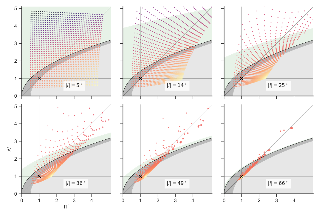
A complementary view of the effects of projection is shown in Figure 12, which shows “snapshots” of $(\Pi^{\prime},\Lambda^{\prime})$ for a sequence of 6 values of the inclination, equally spaced in $\lvert\sin{i}\rvert$, so that each panel is equally likely for an isotropic distribution of orientations. The distribution of the true $\Pi$ and $\Lambda$ are each assumed to be uniform on the range $[0.5,4.5]$, giving a uniformly filled square of values for $\lvert i\rvert=0$, which becomes increasingly distorted as $\lvert i\rvert$ increases. The color scale represents $\mathcal{Q}$ and the symbol size is proportional to $R_{0}^{\prime}/R_{0}$. It can be seen that the points tend to cluster closer and closer to the diagonal, $\Lambda^{\prime}=\Pi^{\prime}$, as the inclination increases, and that the points just below this line tend to have the largest values of $R_{0}^{\prime}/R_{0}$. The green shaded region shows the zone of true $\Lambda,\Pi$ for hyperboloids where the tangent lines still exists for that value of $\lvert i\rvert$. This becomes smaller and smaller as $\lvert i\rvert$ increases, which explains why the hyperboloid zone becomes increasingly depopulated: all quadrics that lay above this region when $i=$$$ will no longer be visible as a bow for this value of $\lvert i\rvert$. Note that this figure is merely illustrative of the qualitative effects of projection, since in reality there is no particular reason to expect a uniform distribution in true $\Pi$ and $\Lambda$.

We wish to generalize the results of Canto et al. (1996, CRW ) to the case where the inner wind is no longer isotropic, but instead has a density that falls off with angle, $\theta$, away from the symmetry axis. Specifically, at some fiducial spherical radius, $R_{0}$, from the origin, the wind mass density is given by

where $\rho_{0}$ is the density on the symmetry axis and $k\geq 0$ is an anisotropy index. The wind velocity is still assumed to be constant and the wind streamlines to be radial, so the radial variation of density at each angle is $\rho(R,\theta)=\rho(R_{0},\theta)\,(R/R_{0})^{-2}$ and the wind mass loss rate and momentum loss rate per solid angle both have the same $\cos^{k}\theta$ dependence as the density. Examples are shown in Figure 13 for a variety of different values of $k$. As $k$ increases, the wind becomes increasingly jet-like.

Our primary motivation for considering such an anisotropic wind is the case of the Orion Nebula proplyds and their interaction with the stellar wind of the massive star $\theta^{1}$ Ori C (García-Arredondo et al., 2001). The inner “wind” in this case is the transonic photoevaporation flow away from a roughly hemispherical ionization front, where photoionization equilibrium, together with monodirectional illumination of the front, implies that the ionized hydrogen density, $n$, satisfies $n^{2}\propto\cos\theta$, which is equivalent to $k=0.5$ in equation (57). Since the primary source of ionizing photons is the same star that is the source of the outer wind, it is natural that the inner wind’s axis should be aligned with the star–star axis in this case. For other potential causes of wind anisotropy (for instance, bipolar flow from an accretion disk), there is no particular reason for the axes to be aligned, so cylindrical symmetry would be broken. Nevertheless, we calculate results for general $k$ with aligned axes, so as to provide a richer variety of cylindrically symmetric bow shock shapes than are seen in the cantoids.

The general solution for the bow shock shape, $R(\theta)$, in the 5 formalism is

where $\dot{\Pi}_{\mathrm{w}{}r}$, $\dot{\Pi}_{\mathrm{w}{}z}$, $\dot{J}_{\mathrm{w}}$ are the accumulated linear radial momentum, linear axial momentum, and angular momentum, respectively, due to the inner wind emitted between the axis and $\theta$. The equivalent quantities for the outer wind have subscripts appended with “1”. The inner wind momenta for our anisotropic case (replacing 5’s eqs. [9, 10]) are:

where

is the total mass-loss rate of the inner wind. The integral

has an analytic solution in terms of the hypergeometric function, ${}_{2}F_{1}(-\tfrac{1}{2};\tfrac{1+k}{2};\tfrac{3+k}{2};\cos^{2}\theta)$, but is more straightforwardly calculated by numerical quadrature. The angular momentum of the inner wind about the origin is $\dot{J}_{\mathrm{w}}=0$ because it is purely radial. The outer wind momenta are unchanged from the 5 case, but are given here for completeness:

We define $\beta$ in this case as the momentum ratio on the symmetry axis, which means that

Substituting equations (59–63) into equation (58) and making use of the geometric relation between the interior angles of the triangle shown in Figure 3:

yields

which is the generalization of 5’s equation (24) to the anisotropic case. Equation (65) is solved numerically to give $\theta_{1}(\theta)$, which is then combined with equations (64) and (1) to give the dimensionless bow shape, $R(\theta;\beta,k)/R_{0}$, where we now explicitly indicate the dependence of the solution on two parameters: axial momentum ratio, $\beta$, and anisotropy index, $k$. We refer to the resultant bow shapes as ancantoids.

The shapes of the ancantoid bow shocks are shown in Figure 14 for three different values of $\beta$, and are compared with the 5 results for cantoids (dashed curves). The location of these shapes in the planitude–alatude plane is shown in Figure 15, where the gray background shading indicates the zones of different quadric classes, as in § 4, Figures 11 and 12. Values of $\Pi$ and $\Lambda$ are calculated via the analytic expressions derived in Appendix D.1 and D.2, respectively, which are only approximate in the case of $\Lambda$. However, the filled square symbols show the exact results for $\beta=0.5$, which can be seen to lie extremely close to the approximate results, even for the worst case of $k=0$. The leading term in the relative error of equation (112) scales as $(\beta/(k+2))^{2}$, so the approximation is even better for smaller $\beta$ and larger $k$.

It is apparent from Figure 14 that the $k=0$ ancantoid is identical to the cantoid for $\theta\leq$$$ ($z>0$, to the right of vertical dotted line in Fig. 14), but is slightly more swept back in the far wings.⁹⁹ 9 Due to the discontinuity in the inner wind density at $\theta=$$$ (see Fig. 13), there is a discontinuity in the second derivative of the bow shape. Since the true planitude and alatude depend on $R(\theta)$ only in the range $\theta=[0,$$]$, the cantoid and the $k=0$ ancantoid behave identically in Figure 15. There is a general tendency for the bows to be flatter and more open with increasing $\beta$ and decreasing $k$, with the cantoid being most open at a given $\beta$. All the models cluster close to the diagonal $\Lambda\simeq\Pi$ in the planitude–alatude plane, but with a tendency for $\Lambda>\Pi$ at higher anisotropy. There is therefore a degeneracy between $\beta$ and $k$ for higher values of $\beta$. The wilkinoid shape, which corresponds to the $\beta\to 0$ limit of the cantoids, is marked by a white plus symbol in Figure 15, and lies in the prolate spheroid region of the plane. Cantoids lie either in the prolate spheroid or hyperboloid regions, according to whether $\beta$ is less than or greater than about $0.01$. For ancantoids of increasing $k$, this dividing point moves to higher values of $\beta$, until almost the entire range of models with $k=8$ are within the prolate spheroid zone.

However, the true planitude and alatude, which are what would be observed for a side-on viewing angle ($i=0$), are not at all sensitive to the behavior of the far wings of the bow shock, which has a rather different implication as to which variety of quadric best approximates each shape. We illustrate this is Figure 16, which shows two different ways of estimating the quadric angle, $\theta_{\mathcal{Q}}$ (see § 4). The first is from $(\Pi,\Lambda)$, as in Figure 15:

which follows from equations (31), (32), and (38). The second is from the asymptotic opening angle of the wings, $\theta_{\infty}$ (Fig. 4):

where $\theta_{\infty}$ is calculated from equation (115) for ancantoids, or (117) for cantoids. If the bow shock shape were truly a quadric, then these two definitions would agree. However, as seen in Figure 16, this is not the case for the cantoids and ancantoids. While $\smash[b]{\theta_{\mathcal{Q}}^{\text{head}}}$ generally corresponds to a prolate spheroid (except for the largest values of $\beta$), $\smash[b]{\theta_{\mathcal{Q}}^{\text{tail}}}$ always corresponds to a hyperbola. This tension between the shape of the head and the shape of the far wings has important implications for the projected shapes (as we will see in the next section), since the far wings influence the projected planitude and alatude when the inclination is large.

Figure 17 shows the parabolic departure function (see § 4.1) for the thin-shell models. This provides an alternative perspective on the resultant bow shapes, with two different types of behavior being apparent. Models with high $\beta$ and low anisotropy behave similarly to the hyperboloids, such as the $(\Pi,\Lambda)=(\nicefrac{{3}}{{2}},\nicefrac{{8}}{{3}})$, $(2,\nicefrac{{8}}{{3}})$, $(\nicefrac{{8}}{{3}},\nicefrac{{8}}{{3}})$, and $(\nicefrac{{3}}{{2}},2)$ cases from Figure 9. This is the case for the $\beta\geq 0.01$ models in Figure 17a, which all show departure functions that become negative in the far wings (more open than parabola) and terminate at a $\theta_{\infty}<$$$. The second type of behavior is shown by models with low $\beta$ or high anisotropy, which behave like spheroids for positive and mildly negative values of $\cos\theta$, but, unlike the spheroids, all tend towards $\Depart=0$ in the far tail as $\cos\theta\to-1$.

Figures 18 and 19 show the apparent bow shapes of various thin shell models (wilkinoid, cantoids, ancantoids)¹⁰¹⁰ 10 See also previous studies of the projected shape of the wilkinoid (Wilkin, 1997; Cox et al., 2012; Ng et al., 2017) and the cantoids (Robberto et al., 2005). for different inclination angles $\lvert i\rvert$. For comparison, Figure 18a shows the confocal paraboloid, whose apparent shape is independent of inclination (see Appendix C). The wilkinoid (Fig. 18b) shows only subtle changes, with the wings becoming slightly more swept back as the inclination increases. The cantoids (Fig. 18c and d) behave in the opposite way, with the wings becoming markedly more open once $\lvert i\rvert$ exceeds $60°$ (for $\beta=0.001$), or $45°$ (for $\beta=0.01$). The ancantoids (Fig. 19) can show more complex behavior. For instance, in the $k=0.5$, $\beta=0.001$ ancantoid (Fig. 19a) the near wings begin to become more closed with increasing inclination up to $\lvert i\rvert=$$$, at which point they open up again, whereas the opening angle of the far wings increases monotonically with $\lvert i\rvert$.

The inclination-dependent tracks that are traced by the thin-shell models in the projected planitude–alatude plane are shown in Figure 20. The behavior is qualitatively different from the quadric shapes shown in Figure 11a in that the tracks are no longer confined within the borders of the region of a single type of quadric (hyperboloid or spheroid). At low inclinations, many of the models behave like the prolate spheroids, but then transition to a hyperboloid behavior at higher inclinations, which is due to the tension between the shape of the head and the shape of the far wings, as discussed in the previous section. This can be seen most clearly in the $\beta=0.001$, $k=0.5$ ancantoid (lowest red line in Fig. 20a, see also zoomed version in Fig. 21). The track begins heading towards $(\Pi^{\prime},\Gamma^{\prime})=(1,1)$, as expected for a spheroid, but then turns around and crosses the paraboloid line to head out on a hyperboloid-like track.

Ancantoids with different degrees of inner-wind anisotropy are shown in Figure 20b. In all cases, the tracks follow hyperboloid-like behavior at high inclinations, tending to populate the region just above the diagonal $\Lambda^{\prime}=\Pi^{\prime}$. The $k=0$ ancantoids show a kink in their tracks at the point where the projected apex passes through $\theta=$$$, due to the discontinuity in the second derivative of $R(\theta)$ there (see footnote 9). The wilkinoid has a much less interesting track, most clearly seen in the zoomed Figure 21, simply moving the short distance from $(\nicefrac{{5}}{{3}},\sqrt{3})$ to $(\nicefrac{{3}}{{2}},\smash{\sqrt{\nicefrac{{8}}{{3}}}})$. Despite its location in the ellipsoid region of the plane, the fact that it has $\theta_{\infty}=$$$ means that it behaves more like a parabola at high inclination, but converges on $(\nicefrac{{3}}{{2}},\smash{\sqrt{\nicefrac{{8}}{{3}}}})$ instead of $(2,2)$ since the far wings are asymptotically cubic, rather than quadratic.

The local density of tick marks gives an indication of how likely it would be to observe each portion of the track, assuming an isotropic distribution of viewing angles. It can be seen that the ticks tend to be concentrated towards the beginning of each track, near the $\lvert i\rvert=0$ point, so the hyperboloid-like portions of the tracks would be observed for only a relatively narrow range of inclinations. This concentration becomes more marked as $\beta$ becomes smaller, which helps to resolve the apparent paradox that the wilkinoid corresponds to the $\beta\to 0$ limit of the cantoids, and yet follows a qualitatively different track. The detailed behavior of the small-$\beta$ cantoid models is shown in Figure 21, which zooms in on the region around the wilkinoid track. It can be seen that for $\beta<0.001$ the cantoid tracks begin to develop a downward hook, similar to the $k=0.5$ ancantoids discussed above. For $\beta<10^{-4}$ this begins to approach the wilkinoid track and the high inclination, upward portion of the track becomes less and less important as $\beta$ decreases.

References

- Astropy Collaboration et al. (2013) Astropy Collaboration et al., 2013, A&A, 558, A33
- Astropy Collaboration et al. (2018) Astropy Collaboration et al., 2018, AJ, 156, 123
- Bally et al. (2000) Bally J., O’Dell C. R., McCaughrean M. J., 2000, AJ, 119, 2919
- Bally et al. (2006) Bally J., Licht D., Smith N., Walawender J., 2006, AJ, 131, 473
- Canto et al. (1996) Canto J., Raga A. C., Wilkin F. P., 1996, ApJ, 469, 729
- Cox et al. (2012) Cox N. L. J., et al., 2012, A&A, 537, A35
- García-Arredondo et al. (2001) García-Arredondo F., Henney W. J., Arthur S. J., 2001, ApJ, 561, 830
- Gayley (2009) Gayley K. G., 2009, ApJ, 703, 89
- Gfrerrer & Zsombor-Murray (2009) Gfrerrer A., Zsombor-Murray P., 2009, Journal for Geometry and Graphics, 13, 131
- Goldman (1983) Goldman R., 1983, IEEE Computer Graphics and Applications, 3, 68
- Graham et al. (2002) Graham M. F., Meaburn J., Garrington S. T., O’Brien T. J., Henney W. J., O’Dell C. R., 2002, ApJ, 570, 222
- Guggenheimer (2012) Guggenheimer H., 2012, Differential Geometry. Dover Books on Mathematics, Dover Publications
- Gutiérrez-Soto (2015) Gutiérrez-Soto L. Á., 2015, Master’s thesis, Universidad Nacional Autónoma de México
- Hartigan et al. (1987) Hartigan P., Raymond J., Hartmann L., 1987, ApJ, 316, 323
- Hayward et al. (1994) Hayward T. L., Houck J. R., Miles J. W., 1994, ApJ, 433, 157
- Henney (2002) Henney W. J., 2002, Revista Mexicana de Astronomia y Astrofisica, 38, 71
- Henney et al. (2013) Henney W. J., García-Díaz M. T., O’Dell C. R., Rubin R. H., 2013, MNRAS, 428, 691
- Jones et al. (2019) Jones E., Oliphant T., Peterson P., et al., 2001–2019, SciPy: Open source scientific tools for Python, http://www.scipy.org/
- Joye & Mandel (2003) Joye W. A., Mandel E., 2003, in Payne H. E., Jedrzejewski R. I., Hook R. N., eds, Astronomical Society of the Pacific Conference Series Vol. 295, Astronomical Data Analysis Software and Systems XII. p. 489
- Kobulnicky et al. (2010) Kobulnicky H. A., Gilbert I. J., Kiminki D. C., 2010, ApJ, 710, 549
- Kobulnicky et al. (2016) Kobulnicky H. A., et al., 2016, ApJS, 227, 18
- Mackey et al. (2012) Mackey J., Mohamed S., Neilson H. R., Langer N., Meyer D. M.-A., 2012, ApJ, 751, L10
- Mackey et al. (2015) Mackey J., Gvaramadze V. V., Mohamed S., Langer N., 2015, A&A, 573, A10
- Markevitch et al. (2002) Markevitch M., Gonzalez A. H., David L., Vikhlinin A., Murray S., Forman W., Jones C., Tucker W., 2002, ApJ, 567, L27
- Meaburn et al. (2013) Meaburn J., Boumis P., Akras S., 2013, MNRAS, 435, 3462
- Medina et al. (2014) Medina S.-N. X., Arthur S. J., Henney W. J., Mellema G., Gazol A., 2014, MNRAS, 445, 1797
- Meyer et al. (2014) Meyer D. M.-A., Mackey J., Langer N., Gvaramadze V. V., Mignone A., Izzard R. G., Kaper L., 2014, MNRAS, 444, 2754
- Meyer et al. (2016) Meyer D. M.-A., van Marle A.-J., Kuiper R., Kley W., 2016, MNRAS, 459, 1146
- Meyer et al. (2017) Meyer D. M.-A., Mignone A., Kuiper R., Raga A. C., Kley W., 2017, MNRAS, 464, 3229
- Mohr & Phillips (2015) Mohr P. J., Phillips W. D., 2015, Metrologia, 52, 40
- Ng et al. (2017) Ng C.-Y., Bandiera R., Hunstead R. W., Johnston S., 2017, ApJ, 842, 100
- O’Dell & Wen (1994) O’Dell C. R., Wen Z., 1994, ApJ, 436, 194
- Ochsendorf et al. (2014) Ochsendorf B. B., Verdolini S., Cox N. L. J., Berné O., Kaper L., Tielens A. G. G. M., 2014, A&A, 566, A75
- Penrose (2004) Penrose R., 2004, The road to reality : a complete guide to the laws of the universe. Jonathan Cape, London
- Phillips et al. (2010) Phillips J. P., Cuesta L. C., Ramos-Larios G., 2010, MNRAS, 409, 881
- Quincey & Brown (2017) Quincey P., Brown R. J. C., 2017, Metrologia, 54, 454
- Raga et al. (1990) Raga A. C., Binette L., Canto J., Calvet N., 1990, ApJ, 364, 601
- Ricci et al. (2008) Ricci L., Robberto M., Soderblom D. R., 2008, AJ, 136, 2136
- Robberto et al. (2005) Robberto M., et al., 2005, AJ, 129, 1534
- Scherer & Fichtner (2014) Scherer K., Fichtner H., 2014, ApJ, 782, 25
- Schwartz (1978) Schwartz R. D., 1978, ApJ, 223, 884
- Shu et al. (2002) Shu F. H., Lizano S., Galli D., Cantó J., Laughlin G., 2002, ApJ, 580, 969
- Smith et al. (2005) Smith N., Bally J., Shuping R. Y., Morris M., Kassis M., 2005, AJ, 130, 1763
- Stevens et al. (1992) Stevens I. R., Blondin J. M., Pollock A. M. T., 1992, ApJ, 386, 265
- Tenorio-Tagle (1979) Tenorio-Tagle G., 1979, A&A, 71, 59
- Weisstein (2018) Weisstein E. W., 1999–2018, Radius of Curvature, From MathWorld – A Wolfram Web Resource., http://mathworld.wolfram.com/RadiusofCurvature.html
- Wilkin (1996) Wilkin F. P., 1996, ApJ, 459, L31
- Wilkin (1997) Wilkin F. P., 1997, PhD thesis, University of California, Berkeley
- Wilkin (2000) Wilkin F. P., 2000, ApJ, 532, 400
- Wilson & Ulvestad (1987) Wilson A. S., Ulvestad J. S., 1987, ApJ, 319, 105
- Zank (1999) Zank G. P., 1999, Space Sci. Rev., 89, 413
- de Sterck & Poedts (1999) de Sterck H., Poedts S., 1999, A&A, 343, 641
- van Buren & McCray (1988) van Buren D., McCray R., 1988, ApJ, 329, L93
- van Dyke (1982) van Dyke M., 1982, An album of fluid motion. Parabolic Press, Stanford, CA
- van Marle et al. (2011) van Marle A. J., Meliani Z., Keppens R., Decin L., 2011, ApJ, 734, L26
Appendix A Radius of curvature
The radius of curvature of a general curve can be written (e.g., eq. [2-5] of Guggenheimer, 2012):