ARTICLE
A SURVEY OF A HURDLE MODEL FOR HEAVY-TAILED DATA BASED ON THE GENERALIZED LAMBDA DISTRIBUTION
D. Marcondes†, C. Peixoto† and A. C. Maia‡
† Instituto de Matemática e Estatística, Universidade de São Paulo, Brazil
‡ Faculdade de Economia, Administraçção e Contabilidade, Universidade de São Paulo, Brazil
dmarcondes@ime.usp.br
Key Words: Generalized Lambda Distribution, Generalized Pareto Distribution, hurdle models, two-way models.
ABSTRACT
In this survey we present an extensive research of the vast literature about the Generalized Lambda Distribution (GD) and propose a hurdle, or two-way, model whose associated distribution is the GD in order to meet the demand for a highly flexible model of heavy-tailed data with excess of zeros. We apply the developed models to a dataset consisting of yearly healthcare expenses, a typical example of heavy-tailed data with excess of zeros. The fitted models are compared with models based on the Generalised Pareto Distribution and it is established that the GD models perform best.
1. INTRODUCTION
A motivation for the development of models for heavy-tailed data with excess of zeros arises from data on healthcare expenses, that is characterized by its heavy tails, its great number of zeros and its high skewness, which makes fitting models to it a complex task (Mihaylova et al., (2011); Jones et al., (2014)). Indeed, a suitable choice of model for healthcare expenses are clumped-at-zero models, that are those with excess of zeros. The clumped-at-zero models are divided into two classes, as follows. The first class are the zero-inflated models, which are based on distributions that already have a probability mass at zero, that is then inflated. The zero-inflated Poisson model is an element of this class (Lambert, (1992)). The second class of clumped-at-zero models are the two-part or hurdle models, that are those whose underlying distribution does not have a probability mass at zero, that is then added to it. They are called hurdle for the probability mass at zero may be seem as a hurdle. In the same sense, they are also known as two-part models because the probability mass at zero and the non-zero values may be modelled independently of each other, i.e., the model has two parts. An example of hurdle model, for the demand of medical care, is presented in Duan et al. ((1983)). In the class of two-part models there are also models whose underlying distribution has a probability mass at zero, but are nonetheless two-part models, as the model of Mullahy ((1986)), since the inflation of the probability mass at zero is made independently of the non-zero data by truncation.
The underlying distribution of the hurdle model treated in this paper is the Generalized Lambda Distribution (GD), that is a highly flexible four-parameter continuous probability distribution. This distribution was first proposed by Ramberg & Schmeiser ((1974)), and then extended by Freimer et al. ((1988)), as a generalization of Tukey’s Lambda Distribution (Hastings et al., (1947); Tukey, (1990)). Even though the GD is a wild card distribution, that well approximate others (Karian & Dudewicz, (2000), Chapter 3), its use has been limited in the literature as there is no explicit expression for its probability density function, which makes it a complex task to estimate its parameters.
Indeed, the estimation of the parameters of the GD had been carried out by the methods of moments and a percentile method until Su ((2007)) proposed a numerical maximum likelihood method for it. Another limitation for the use of the GD was the lack of a regression model, that was just recently proposed by Su ((2015)), which extended the range of applications for the GD. Therefore, due to recent advances in the theory of the GD, it is now possible to further apply this powerful distribution and compare it to other established models in order to assess its advantages.
Although the estimation techniques for the GD have been limited, there is a considerable amount of applications of it in the literature. As examples, we cite the evaluation of non-normal process capability indices (Pal, (2004)), option pricing (Corrado, (2001)), the fitting of solar radiation data (Öztürk & Dale, (1982)) and income data (Tarsitano, (2004)), and statistical process control (Fournier et al., (2006)). Regarding the modelling of healthcare expenses, the GD was studied by Balasooriya & Low ((2008)), where it was compared with the transformed kernel density and models of the exponential family, and it was established that the GD fitted the data best.
In this paper, we develop hurdle GD models and assess their goodness-of-fit on a yearly healthcare expenses dataset. The models developed seek to fit the data taking into account covariates (regression model) or not. The GD models are compared with hurdle models based on the Generalized Pareto Distribution (GPD), that are special cases of the model in Couturier & Victoria-Feser ((2010)). The GPD is also a highly flexible continuous probability distribution, although we argue that it is not as flexible as, and do not fit the data as good as, the GD. For an assessment of the goodness-of-fit of the GPD for healthcare expenses see Cebrián et al. ((2003)).
In Section 2 we present a survey about the GD and its estimation techniques. In Section 3 we propose a hurdle GD and develop its main properties. In Section 4 we present a survey about GD regression models, and develop a hurdle GD regression model. In Section 5 we present a simulation study about the asymptotic properties of the hurdle GD regression coefficients. In Section 6 we apply the developed methods to model healthcare expenses and compare GD models and GPD models.
2. THE GENERALIZED LAMBDA DISTRIBUTION
In this section we present two distinct parametrizations of the GD, known as the RS and FKML GD, and some of their properties.
2.1 RS GENERALIZED LAMBDA DISTRIBUTION
The RS GD, as proposed by Ramberg & Schmeiser ((1974)), is a four parameter generalization of Tukey’s Lambda Distribution, obtained from an uniform random variable. Let be an uniform random variable with range defined in a probability space . Then, the random variable , also defined in , and given by
| (1) |
has an RS GD with parameters . The function , is the quantile function of as , in which . The density of is given by
| (2) |
in which is the derivative of at point . The parametric space is a cumulative distribution function of is a proper subset of and is given implicitly by inequality
| (3) |
for . The inequality is obtained noting that if, and only if, .
The RS GD is quite flexible, as it is possible to specify its parameters in order to obtain a specific distribution with given mean, variance, skewness and kurtosis. Indeed, the mean can be shifted to any value by choosing properly, the skewness and kurtosis are determined by and and, given and , the variance is determined by . The range of is and depends on (see Karian & Dudewicz ((2000), Theorem 1.4.23) for the RS GD range). The kth moment of the RS GD exists if, and only if, and, when it exists and , it is given by
| (4) |
in which is the beta function evaluated at . A proof for (4) is given in Ramberg & Schmeiser ((1974)). The central moments of when may be obtained from (4) by applying the properties of the expectation operator. For instance, we have that
| (5) |
so that if, and only if, and is symmetric.
The estimation of the RS GD parameters may be performed by various methods. The classical estimation technique is the Method of Moments (MM), as introduced by Ramberg & Schmeiser ((1974)) and consolidated by Karian et al. ((1996)). Although easily implemented nowadays, the MM has some limitations. First of all, two different vectors may yield the same first four moments of the RS GD. As pointed out by Karian et al. ((1996)) it may be seen as a problem or an opportunity, for it enables a flexible fit for the data, as we may choose the parameters that best fulfil our objectives regarding the fit. Another limitation of the MM is the fact that the existence of the first four moments depends on and, therefore, it cannot be applied for a subset of . Furthermore, simulation studies have showed that the MM performs worse than other methods, as the Numerical Maximum Likelihood Method (NMLM) and the percentile matching approach, for example (Karian & Dudewicz, (2003); Su, (2007)).
Even though other methods, as the least square estimation method proposed by Öztürk & Dale ((1985)), the Starship Method developed by King & MacGillivray ((1999)), the flexible discretized approach proposed by Su ((2005)) and the percentile matching approach, similar to the MM but with best results in simulation studies, as introduced by Karian & Dudewicz ((1999)) and further studied by Karian & Dudewicz ((2000)) and Karian & Dudewicz ((2003)), are available in the literature, this paper treats only estimation by the NMLM, as proposed by Su ((2007)) and Su ((2011)). For a good account of other estimation techniques see Lakhany & Mausser ((2000)).
The log-likelihood of a sample of an RS GD random variable may be written in terms of the cumulative distribution function , by denoting , so that
| (6) |
In order to maximize (6) it is preferable to apply direct numerical methods than the usual method of differentiation, as they are much more reliable and efficient than solving the conventional linear equations on , because, in many cases, the RS GD may be undefined for certain parameters values, as was pointed out by Su ((2011)). Therefore, we apply the algorithm proposed by Su ((2007)) to maximize (6).
The main issue in maximizing (6) is in finding suitable initial values for the quantile sample . The most efficient way of obtaining initial values for them is through the estimation of by the percentile method, as this is the method that, apart from the NMLM, has had more efficient results estimating the RS GD parameters (Karian & Dudewicz, (2003)). The percentile method, as presented in Karian & Dudewicz ((2000)) and Su ((2007)), is as follows. The pth percentile of a sample is defined as , in which is the sample ordered in ascending order and is the greatest integer lesser than , with . Rather than matching the sample moments to their theoretical value, in the percentile method we match the statistics
| (7) |
to their theoretical values, in which is an arbitrary number between and , that we choose to be , so that it is consistent with Karian & Dudewicz ((2000)) and Su ((2007)).
Matching the theoretical values of and to the quantile function of an RS GD we obtain the following relations between and :
| (8) |
The conditions , , and must be satisfied, as can be established from (7). In order to estimate we match the sample values (7) to their theoretical values (8) and solve numerically for by the Newton-Raphson method, for example, with the stopping rule given by the minimization of the Euclidean 2-norm . Once and are obtained from the last two equations of (8), we may substitute their values in the first two equations of (8) in order to obtain and .
The percentile method is applied to get initial values in order to maximize (6). The maximization of (6) is performed by a 4-step algorithm proposed by Su ((2007))11 1 The algorithm in Su ((2007)) has five steps, that we reduced to four, without loss of content., that uses quasi random numbers and the percentile method. The algorithm is as follows:
- 1.
Specify the range of initial values for and and the number of values to be selected. In this step, quasi random numbers are sampled as candidates for the initial values of and . Su ((2007)) proposes that quasi random values (scrambled so that the sampled values fill uniformly the considered space) be chosen from the square .
- 2.
Evaluate for each of the initial values of in the first two equations of (8). Remove all initial values that
- (a)
Do not result in a legal parametrization of the RS GD by (3).
- (b)
Do not span the entire region of the dataset.
Among the initial points not excluded by step , find the initial set that minimizes the norm .
- (a)
- 3.
Calculate the quantiles by solving numerically (1) with the initial values .
- 4.
Once is obtained, substitute them in (6) and solve it numerically for . It is convenient to repeat this process for different initials values, in order to check the consistency of the solution. The obtained estimator is called revised percentile estimator of the RS GD under maximum likelihood estimation. The quality of the final fitting may be established by diagnostic techniques, as the data histogram superimposed by the estimated density, quantile plots and goodness-of-fit tests.
2.2 FKML GENERALIZED LAMBDA DISTRIBUTION
The FKML GD, as proposed by Freimer et al. ((1988)), is also a four parameter generalization of Tukey’s Lambda Distribution obtained from an uniform distribution. Indeed, let be an uniform random variable with range defined in a probability space . Then, the random variable , also defined in , and given by
| (9) |
has an FKML GD with parameters . The FKML GD is a probability distribution for all real-valued parameters , with the restriction that and the conventions that and . The main motivation for generalizing Tukey’s Lambda distribution to (9) is the weaker restrictions on its parametric space when comparing to the RS GD, which facilitates the estimation of its parameters. Although both the RS and FKML GD are generalizations of Tukey’s Lambda Distribution, they are not equivalent, so the distribution fitted by one parametrization to a dataset differs in general from the one fitted by the other.
The range of is dependent on the parameters and is given by . The density of the FKML GD is obtained in a similar manner of (2) and is given by
| (10) |
The distribution of is symmetric if, and only if, , although its skewness measure may be zero for22 2 This is also the case for the RS GD. . The parameters and determine single-handedly the nature and shape of the left and right tails of , respectively, although the shape of the probability density function depends on both and . Examples of FKML GD may be found in Su ((2015)). Although the parameters of both the RS and FKML GD are denoted by , , and , and are related to the same properties of the distribution, they are not equivalent, nor comparable.
The kth moment of the FKML GD also exists if, and only if, . Making and , the kth moment of may be obtained from the moments of that, when exist, are given by
| (11) |
as showed in Freimer et al. ((1988)) and Lakhany & Mausser ((2000)). The central moments of may also be obtained from (11).
The FKML GD is also highly flexible, as it is possible to choose so that has specific mean, variance, skewness and kurtosis. Furthermore, its tails are also flexible, so that the FKML GD (and the RS GD) provides a better fit for heavy tailed data than the usual Generalized Additive Models for Location, Scale and Shape (Rigby & Stasinopoulos, (2005)), for example. However, the FKML GD probability density function does not have an analytic form that does not depend on , what calls for computational tools in order to fit it to a dataset.
Although there is also a vast literature about the estimation of the FKML GD parameters, we treat only the NMLM as proposed by Su ((2007)) and Su ((2011)). The log-likelihood of a sample of an FKML GD is given by
| (12) |
in which . The maximization of (12) is performed applying an algorithm slightly different from the one applied to maximize (6). The main issue in maximizing (12) is also in finding initial values for . The estimation method, apart from the NMLM, that seems to perform best under the FKML GD is the method of moments, as outlined by the simulation studies of Lakhany & Mausser ((2000)). Therefore, this is the method we use to find the initial values of in a similar manner of what has been done for the RS GD .
The method of moments for the FKML GD, as presented in Lakhany & Mausser ((2000)), consists on matching the first four sample moments of given by
| (13) | ||||||
to their theoretical moments
| (14) | ||||||
As proposed by Lakhany & Mausser ((2000)), we first solve numerically for and in the plane by the minimization of the Euclidean 2-norm , and then substitute their values in the first two equations of (14) to obtain and . Using the estimates from the method of moments as initial values, we apply an algorithm analogous to the one applied to the RS GD in order to obtain NMLM estimates. The algorithm was also proposed by Su ((2007)), and is a slight modification of the algorithm of Section 2.1, in which the method of moments is used to find the initial values instead of the percentile method, and the FKML GD likelihood is maximized, instead of the RS GD one. More details about it may be found in Su ((2007)).
3. HURDLE GENERALIZED LAMBDA DISTRIBUTION
In this section we propose a Hurdle Generalized Lambda Distribution (HGD) for both the RS and FKML GD parametrizations, and an estimation technique for its parameters. The HGD is obtained by adding a fifth parameter to either the RS or FKML GD that represents their probability mass at zero, so that the hurdle HGD is a mixed probability distribution.
3.1 HURDLE RS GENERALIZED LAMBDA DISTRIBUTION
Let and be independent random variables defined in , such that is uniformly distributed in and . We say that the random variable given by
| (15) |
has a hurdle RS GD (HRS GD) with parameters in the parametric space .
The random variable follows a mixed probability distribution, that has a probability mass at zero and a probability mass spread over according to an RS GD. As the flexibility of the GD is maintained in our hurdle generalization, an advantage of fitting an HRS GD is that it is suitable for modelling data with heavy tails and skewness that also has a great quantity of zeros.
3.1.1 ESTIMATION
The estimation of the HRS GD parameters may be performed by the NMLM with an extension of the method of Su ((2007)). We may represent a sample of by , in which are the observed values and33 3 is the indicator function. , , so that the log-likelihood of is given by
| (16) |
in which
As the log-likelihood (16) may be factored into two functions, one depending on and other depending on , the parameters and are orthogonal and, therefore, may be estimated independently.
The maximum likelihood estimator of is . On the other hand, may be estimated by applying the algorithm of Section 2.1 to the non-zero data values, so that we obtain the revised percentile estimator of the HRS GD under maximum likelihood estimation. As fits the zero data values perfectly, it is enough to apply diagnostic techniques to the non-zero data values, e.g., by comparing graphically their histogram with the density of an RS GD with parameters .
3.2 HURDLE FKML GENERALIZED LAMBDA DISTRIBUTION
The hurdle FKML GD (HFKML GD) is constructed in the same manner as the HRS GD, by letting and be independent random variables defined in , such that is uniformly distributed in and , and defining the random variable as
| (17) |
so that has an HFKML GD with parameters with the restriction that and the same conventions of (9). The random variable also follows a mixed probability distribution with the same general characteristics of the HRS GD: it is highly flexible, has a probability mass at zero and a probability mass spread over according to an FKML GD.
3.2.1 ESTIMATION
The estimation of the HFKML GD is performed in a way analogous to that of the HRS GD, as the log-likelihood of an HFKML GD sample , , may be written as
| (18) |
in which
so that the parameters and are orthogonal, and may be estimated independently.
In order to obtain the revised method of moments estimator of the HFKML GD under maximum likelihood estimation, we estimate by the proportion of zero-valued data and by the algorithm of Section 2.1, using only the non-zero data values. Diagnostic methods may be applied to the non-zero data values in order to assess the quality of the obtained fit.
4. HURDLE GENERALIZED LAMBDA DISTRIBUTION REGRESSION
In this section we propose a regression model for the HGD, in which we model its location and probability mass at zero as functions of covariates and , respectively, which are random vectors defined in , that may share some variables or be equal. Our method is an adaptation of the one presented in Su ((2015)). We first outline the method of Su ((2015)) and then extend it to the HGD.
4.1 FLEXIBLE PARAMETRIC QUANTILE REGRESSION MODEL
The algorithm of Su ((2015)) seeks to estimate of the model
| (19) |
in which and is such that , i.e.,
| (20) |
In order to estimate the parameters of (19) we apply a 5-step algorithm that is analogous to the algorithms of Section 2.1: find initial values to the parameters in order to evaluate and maximize the log-likelihood to get NMLM estimates. It is supposed that we have a sample of the response variable and covariates. The algorithm is as follows and more details about it are presented in Su ((2015)).
- 1.
Obtain from the least square method by solving
and calculate the initial residuals .
- 2.
Obtain the initial estimates by applying the algorithm of Section 2.1 to sample of .
- 3.
Calculate the log-likelihood of the model as follows:
- (a)
Evaluate by (20) so that the initial estimated distribution of the error has zero mean.
- (b)
Force the residuals sample mean to be zero by making
- (c)
- (a)
- 4.
Maximize numerically, by the Nelder-Mead simplex algorithm (Nelder & Mead, (1965)), for example, the log-likelihood (21) or (23), depending on the parametrization, using and as initial values, in order to obtain and .
- 5.
Obtain substituting the estimated values and in (20).
- 6.
Conduct simulations to obtain statistical properties of the estimated regression coefficients as follows:
- (a)
Generate from the GD with parameters and obtain a new sample by adding . Fit a regression model to obtaining estimates for the regression coefficients.
- (b)
Repeat step (a) times to obtain coefficients44 4 The number is arbitrary. It could be sampled more or less coefficients..
- (c)
Adjust the each coefficient sample in (b) so that its mean is equal to the final estimated coefficients of step 5. The simulated coefficients histogram may be plotted and confidence intervals may be found by evaluating the and quantiles of the simulated samples. We use quantile type 8 from the quantile function in R (Hyndman & Fan, (1996); R Core Team, (2017)) in order to be consistent to Su ((2015)).
- (a)
Any other method could be used to estimate the parameters of the error distribution in step 2. However, we prefer the NMLM for it provides better estimates, as has been established on the literature, although it may not converge in some cases. A limitation of this method is the lack of asymptotic theoretical results about the distribution of the estimators, so that we cannot construct asymptotic confidence intervals, nor test hypothesis, for the coefficients. Nevertheless, computational methods for generating confidence intervals for the coefficients and for establishing goodness of fit are implemented and can be applied (Su, (2016)).
4.2 HGD REGRESSION MODEL
In order to develop an HGD regression model, we rely on the factorization of the log-likelihoods (16) and (18), as it allows to model the parameter and the location of the distribution independently. Indeed, our regression model, whose response variable is and covariates are55 5 Note that and may share some of the same variables or be equal. , may be written as
| (25) |
in which and is such that , i.e., is given by relation (20).
Given a sample of model (25), in which , the log-likelihood of the parameters is given by
| (26) |
in which is either the density (2) or (10) with parameters evaluated at point .
The estimation of the parameters of model (25) may be performed by maximizing and independently, so that we get the maximum likelihood estimator and the NMLM estimators and . On the one hand, the maximization of is performed by fitting a logistic regression in the usual manner, as shown in Hilbe ((2009)) for example, to sample . On the other hand, the maximization of is performed by applying the algorithm of Section 4.1 to the non-zero data values.
As the parameters and are orthogonal, their maximum likelihood estimators are asymptotically independent (Cox & Reid, (1987)). Therefore, the usual methods of inference for logistic regression models may be applied to infer about . Similarly, logistic regression diagnostic techniques may also be applied in order to asses the quality of the fit. However, as the estimators and are not of maximum likelihood, the usual inference techniques for maximum likelihood estimators cannot be applied to them. Nevertheless, we may construct numerical confidence intervals for by applying the method of step 6 of algorithm of Section 4.1 to the non-zero data values.
The goodness-of-fit of HGD regression models may be established by the study of two kinds of residuals: error residuals and normalized quantile residuals. The error residuals are given by for all and their empirical distribution may be compared with the GD, that was fitted to the error in order to establish goodness-of-fit. This comparison may be performed by the use of QQ-plots, a histogram of superimposed by the estimated density and a quantile plot that superimposes the estimated and the empirical quantile functions of and , respectively.
The normalized quantile residuals, as presented, for example, in Dunn & Smyth ((1996)), are defined as , in which and are the cumulative distribution function of the standard normal distribution and the RS or FKML GD, respectively. The normalized quantile residuals are expected to be normally distributed if the model is properly fitted, so that we may regard the model as well fitted if the density estimate of is close to the standard normal distribution density and the points of the normal QQ-plot of are distributed around the line with intercept zero and slope one, for example. These residuals may also be used to asses the goodness-of-fit of the logistic regression model (Rigby & Stasinopoulos, (2005)).
5. SIMULATION STUDY
In this section we perform a simulation study in order to assess the asymptotic properties of the HGD regression models. We consider the model
| (27) |
in which and . We consider four different scenarios in our simulations, in which the distribution of the error is symmetric (RS GD(0,2,0.13,0.13) and FKML GD(0,2,0.13,0.13)), and right skewed (RS GD(-1.43,0.11,0.0023,0.19) and FKML GD(-0.147,-0.41,1.07,0.84,0.02)). In each scenario, we generate samples of model (27), for each sample size and , and, for each sample, we fit a HGD regression model, estimating the coefficients of (27). We them study the mean, standard error and the 2.5th and 97.5th percentiles of the estimated coefficients of (27) over samples. The results are presented in Table 1.
We observe that, in all scenarios, the mean of the estimated coefficients is close to the target value, especially for the sample of size , which is evidence that the estimators are unbiased. Furthermore, we see that as greater the sample size is, smaller is the standard error of the estimated coefficients, which is evidence that the estimators are consistent. Overall, the simulation study support the consistency of the estimators, so that it is not lost when we consider the hurdle model: the logistic regression consistency, theoretically established, and the consistency of the GD regression, supported by the simulations of Su ((2015)), seems to be preserved when we consider the hurdle model.
| Distribution of | Coefficient | Target | Sample | Mean | Standard | Percentiles | |
|---|---|---|---|---|---|---|---|
| Size | Error | 2.5th | 97.5th | ||||
| Non-zero intercept | 6.12 | 100 | 6.131 | 0.091 | 5.959 | 6.309 | |
| 200 | 6.130 | 0.059 | 6.009 | 6.244 | |||
| 1,000 | 6.130 | 0.022 | 6.085 | 6.174 | |||
| Non-zero | -0.021 | 100 | -0.021 | 0.016 | -0.052 | 0.008 | |
| 200 | -0.021 | 0.010 | -0.040 | 0.001 | |||
| 1,000 | -0.021 | 0.004 | -0.028 | -0.013 | |||
| Non-zero | -0.35 | 100 | -0.350 | 0.048 | -0.446 | -0.255 | |
| 200 | -0.350 | 0.033 | -0.416 | -0.284 | |||
| HRS | 1,000 | -0.350 | 0.012 | -0.375 | -0.326 | ||
| GD(0,2,0.13,0.13) | Zero intercept | 1.6 | 100 | 1.659 | 0.944 | -0.001 | 3.762 |
| 200 | 1.627 | 0.650 | 0.401 | 2.984 | |||
| 1,000 | 1.611 | 0.272 | 1.097 | 2.136 | |||
| Zero | -0.13 | 100 | -0.136 | 0.164 | -0.464 | 0.191 | |
| 200 | -0.131 | 0.110 | -0.362 | 0.083 | |||
| 1,000 | -0.132 | 0.046 | -0.223 | -0.043 | |||
| Zero | 0.21 | 100 | 0.190 | 0.492 | -0.768 | 1.139 | |
| 200 | 0.207 | 0.341 | -0.481 | 0.829 | |||
| 1,000 | 0.216 | 0.149 | -0.072 | 0.509 | |||
| Non-zero intercept | 6.12 | 100 | 6.145 | 0.750 | 4.615 | 7.664 | |
| 200 | 6.114 | 0.489 | 5.215 | 7.215 | |||
| 1,000 | 6.123 | 0.176 | 5.780 | 6.470 | |||
| Non-zero | -0.021 | 100 | -0.022 | 0.129 | -0.283 | 0.243 | |
| 200 | -0.018 | 0.083 | -0.201 | 0.131 | |||
| 1,000 | -0.020 | 0.029 | -0.077 | 0.034 | |||
| Non-zero | -0.35 | 100 | -0.359 | 0.409 | -1.124 | 0.469 | |
| 200 | -0.353 | 0.266 | -0.876 | 0.165 | |||
| HFKML | 1,000 | -0.346 | 0.094 | -0.532 | -0.158 | ||
| GD(0,2,0.13,0.13) | Zero intercept | 1.6 | 100 | 1.623 | 0.916 | 0.040 | 3.577 |
| 200 | 1.620 | 0.649 | 0.388 | 2.975 | |||
| 1,000 | 1.611 | 0.272 | 1.097 | 2.136 | |||
| Zero | -0.13 | 100 | -0.136 | 0.159 | -0.438 | 0.171 | |
| 200 | -0.131 | 0.108 | -0.362 | 0.081 | |||
| 1,000 | -0.132 | 0.046 | -0.223 | -0.043 | |||
| Zero | 0.21 | 100 | 0.206 | 0.482 | -0.735 | 1.149 | |
| 200 | 0.205 | 0.342 | -0.484 | 0.834 | |||
| 1,000 | 0.216 | 0.149 | -0.072 | 0.509 | |||
| Non-zero intercept | 6.12 | 100 | 6.080 | 0.784 | 4.434 | 7.697 | |
| 200 | 6.102 | 0.448 | 5.200 | 7.003 | |||
| 1,000 | 6.115 | 0.179 | 5.742 | 6.451 | |||
| Non-zero | -0.021 | 100 | -0.014 | 0.134 | -0.273 | 0.300 | |
| 200 | -0.019 | 0.073 | -0.158 | 0.134 | |||
| 1,000 | -0.020 | 0.028 | -0.080 | 0.041 | |||
| Non-zero | -0.35 | 100 | -0.337 | 0.403 | -1.197 | 0.518 | |
| 200 | -0.339 | 0.210 | -0.738 | 0.078 | |||
| HRS | 1,000 | -0.342 | 0.067 | -0.462 | -0.185 | ||
| GD(-1.43,0.11,0.0023,0.19) | Zero intercept | 1.6 | 100 | 1.623 | 0.906 | -0.045 | 3.534 |
| 200 | 1.632 | 0.620 | 0.433 | 2.924 | |||
| 1,000 | 1.616 | 0.273 | 1.068 | 2.152 | |||
| Zero | -0.13 | 100 | -0.131 | 0.160 | -0.442 | 0.188 | |
| 200 | -0.134 | 0.107 | -0.349 | 0.083 | |||
| 1,000 | -0.132 | 0.047 | -0.223 | -0.038 | |||
| Zero | 0.21 | 100 | 0.211 | 0.493 | -0.776 | 1.171 | |
| 200 | 0.209 | 0.328 | -0.447 | 0.848 | |||
| 1,000 | 0.213 | 0.155 | -0.073 | 0.507 | |||
| Non-zero intercept | 6.12 | 100 | 6.139 | 0.777 | 4.584 | 7.906 | |
| 200 | 6.083 | 0.411 | 5.259 | 6.861 | |||
| 1,000 | 6.130 | 0.110 | 5.923 | 6.350 | |||
| Non-zero | -0.021 | 100 | -0.022 | 0.133 | -0.309 | 0.236 | |
| 200 | -0.011 | 0.066 | -0.149 | 0.128 | |||
| 1,000 | -0.021 | 0.015 | -0.050 | 0.011 | |||
| Non-zero | -0.35 | 100 | -0.352 | 0.408 | -1.232 | 0.513 | |
| 200 | -0.366 | 0.187 | -0.742 | 0.019 | |||
| HFKML | 1,000 | -0.351 | 0.042 | -0.446 | -0.268 | ||
| GD(-0.147,-0.41,1.07,0.84,0.02) | Zero intercept | 1.6 | 100 | 1.635 | 0.916 | -0.098 | 3.433 |
| 200 | 1.615 | 0.652 | 0.402 | 2.962 | |||
| 1,000 | 1.613 | 0.279 | 1.054 | 2.154 | |||
| Zero | -0.13 | 100 | -0.132 | 0.157 | -0.434 | 0.187 | |
| 200 | -0.132 | 0.111 | -0.353 | 0.086 | |||
| 1,000 | -0.132 | 0.048 | -0.225 | -0.035 | |||
| Zero | 0.21 | 100 | 0.194 | 0.509 | -0.820 | 1.246 | |
| 200 | 0.200 | 0.338 | -0.459 | 0.847 | |||
| 1,000 | 0.212 | 0.154 | -0.073 | 0.507 | |||
6. FITTING AN HGD TO HEALTHCARE EXPENSES DATA
Healthcare expenses data has some peculiarities which make the HGD a great option for modelling it. Indeed, yearly healthcare expenses data has usually a great number of zeros, normally more than 50% of the data, as not every person uses their health insurance in the period of a year. Furthermore, the distribution of healthcare expenses is highly skewed and has a heavy tail that is hardly modelled by the usual distributions, as the Gamma, Weibull, Log-normal and Inverse-Gaussian.
In the following sections, we fit models to a dataset that contains the yearly expenses of all insured customers of a Brazilian healthcare insurance company between 2006 and 2009. Our analysis focuses on modelling the yearly expenses in function of the covariates age, sex and previous year expenses. All expenses are in Reais66 6 Brazilian currency. (R$) and were deflated to January 2006 value. The HGD models are compared with GPD models in order to establish which model best fits the data.
The GPD, introduced by Pickands ((1975)), is a three parameter positive probability distribution with density
for , in which is the location parameter, is the scale parameter and is the shape parameter. The mean of the GPD is finite only for and is given by
| (28) |
Note that the GPD may be re-parametrized so that is the scale parameter, instead of . Given a sample and a known threshold , the parameters (or ) may be estimated by the Maximum Likelihood Method in the usual manner. See Hosking & Wallis ((1987)) and Grimshaw ((1993)) for more details.
In order to fit a GPD to data when there are covariates, we may use a generalized linear model (GLM) framework, as introduced by Nelder & Baker ((1972)). In this framework, we suppose that the location parameter is known and independent of the covariates, and that the shape parameter is unknown, but is lesser than one and independent of the covariates. Then, we model the mean as , in which are the covariates of the observation and are the coefficients of the model. The coefficients are estimated by Maximum Likelihood numerically and their asymptotic distributions are obtained by the asymptotic properties of Maximum Likelihood Estimators.
A Hurdle Generalized Pareto Distribution (HGPD) model may be developed in a similar manner as the HGD model. Indeed, it is enough to add a parameter to the GPD that represents its probability mass at zero and then estimate the parameters accordingly: the estimate of is the proportion of zeros in the sample and the estimate of is the Maximum Likelihood estimate for the GPD fitted to the non-zero data values. A HGPD GLM is obtained by replacing in expression (25) by a random variable that has a GPD with parameters . The parameters related to the probability mass at zero and to the GPD for the non-zero values are orthogonal, so that their estimation may be performed independently, as was the case of the HGD. This hurdle model is a special case of the Zero-inflated Truncated Generalized Pareto Distribution model introduced by Couturier & Victoria-Feser ((2010)).
In order to establish the goodness-of-fit of the HGPD GLM we may consider the zero and non-zero data values separately. For the zero values we consider logistic regression diagnostic techniques and for the non-zero values we propose the study of two types of residuals: normalised quantile residuals and error residuals, that are given respectively by
in which is the cumulative probability function of a GPD with parameters , for . If the model is well-fitted then is normally distributed and has a GPD with parameters , and , so that graphical tools, as QQ-plots, may be used to establish goodness-of-fit. The error residuals were proposed by Couturier & Victoria-Feser ((2010)) where more details are presented.
6.1 THE DATASET
In order to fit a model to the data at hand, we first observe some systematic behaviour of the data and transform it to obtain a better fit. First of all, there are some yearly expense values that are observed in the dataset hundreds of times, as can be seen in Figure 1, as there are some simple medical procedures that have standardized costs. Those repeated values make it hard to fit a continuous model, as some values have a probability mass greater than zero. Therefore, we consider that any expense less than R$ 100 is zero, i.e., we truncate the yearly expenses at R$ 100, and consider all yearly expenses lesser than R$ 100 to be zero. This truncation is justified by the practical application of the fitted model, as the main interest in modelling healthcare expenses is in properly fitting the tail of the distribution, i.e., the yearly expenses that are dozens of times the expected one, so that low expenses, as those less than R$ 100, may be regarded as zero without any loss for the practical application of the model. Indeed, around 69 % of the dataset has an expense less than R$ 100, although their expenses sum to R$ 2,552,800, that is less then 2% of the total expenses of the dataset, that is R$ 137,382,575.

Truncating the dataset at R$ 100, we have, for each year and for the whole dataset, the proportion of zeros, selected percentiles, mean, standard deviation and maximum expense displayed in Table 2. The percentiles, mean and standard deviation refer to the truncated data, i.e., are calculated considering only data values greater than R$ 100. From Table 2 it can be seen that the 99th percentile is approximately twice the 98th percentile, the same occurring with the 99th and 99.5th percentiles. Furthermore, the 99.9th percentile is around three times the 99.5th percentile and the maximum is up to almost five times the 99.9th percentile, which shows that the dataset has heavy tails, as can be also seen in the box-plots of the logarithm of the yearly expenses in Figure 2.
| Year | 2006 | 2007 | 2008 | 2009 | All data | |
| Size | 70,186 | 71,814 | 73,038 | 74,418 | 289,456 | |
| Percentage of R$ 100 | 60 | 81 | 82 | 51 | 69 | |
| 25 | 195 | 151 | 154 | 249 | 190 | |
| 50 | 367 | 237 | 259 | 514 | 366 | |
| 75 | 807 | 453 | 510 | 1,147 | 830 | |
| 90 | 1,901 | 1,033 | 1,180 | 2,782 | 2,040 | |
| 95 | 3,610 | 2,309 | 2,737 | 5,662 | 4,145 | |
| Percentiles | 96 | 4,412 | 3,035 | 3,632 | 7,123 | 5,186 |
| 97 | 5,756 | 4,227 | 4,950 | 9,593 | 6,878 | |
| 98 | 8,337 | 6,633 | 7,906 | 14,754 | 10,629 | |
| 99 | 15,971 | 13,168 | 15,583 | 27,675 | 20,023 | |
| 99.5 | 28,700 | 22,990 | 29,614 | 50,549 | 35,821 | |
| 99.9 | 106,744 | 61,111 | 68,552 | 151,114 | 116,643 | |
| Maximum | 377,862 | 295,736 | 279,450 | 675,440 | 675,440 | |
| Mean | 1,313 | 870 | 991 | 2,028 | 1,485 | |
| Standard Deviation | 7,082 | 4,689 | 4,898 | 10,966 | 8,387 | |
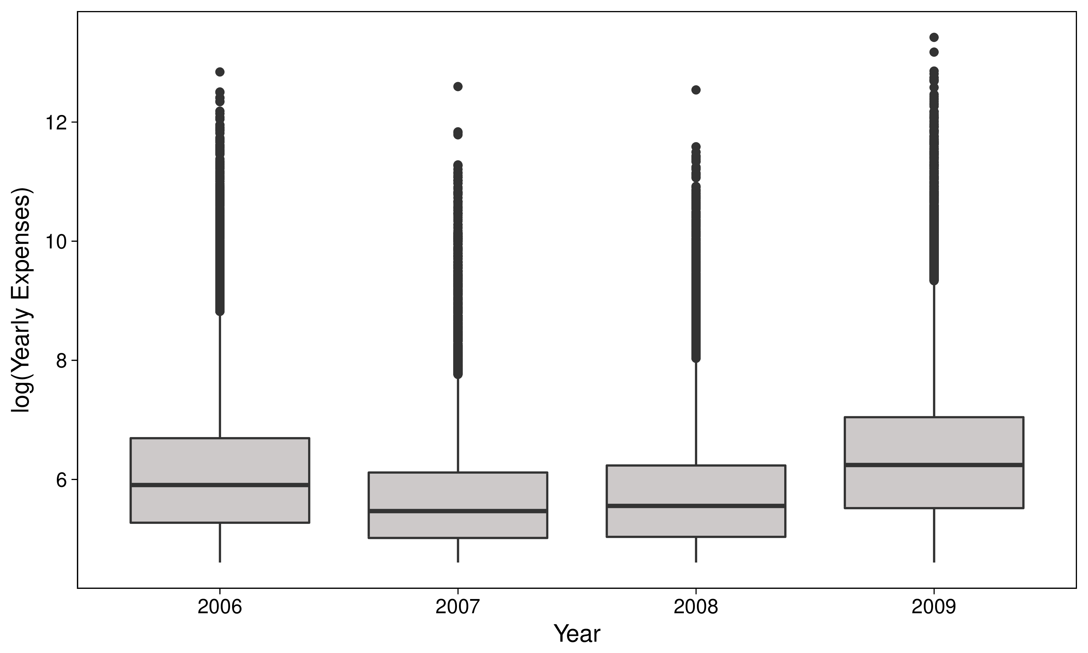
Figure 3 shows the dispersion of the logarithm of the yearly expenses by each of the covariates that are considered on the regression model, i.e., age, sex and the logarithm of the previous year expenses. The data considered for the regression model contemplate the yearly expenses of 2007, 2008 and 2009, and regards only patients that were enrolled in the insurance program in the considered year and in the previous year, which amounts to 214,925 observations. Figure 3 does not yield any clear relation between the logarithm of the yearly expenses and age or previous year expenses, although it seems that women tend to have greater yearly expenses than men.

6.2 HGD MODEL FIT
We first fit HGD and HGPD curves to the yearly expenses of each year (2006, 2007, 2008 and 2009) without considering any covariate. All models are fitted to the logarithm of the yearly expenses in order to obtain better fitted models and for computation optimization, as the non-transformed data has some extreme outliers, which makes it hard to fit a model properly. The goodness-of-fit is established graphically by the use of QQ-plots and the histogram of the data superimposed by the estimated curves. The fitted curves are also compared with the kernel density estimate in order to establish which is the model that best fit the data objectively. See Bickel & Rosenblatt ((1973)) and Fan ((1994)) for examples of how the kernel density estimation is used for assessing goodness-of-fit. We apply the method proposed by Sheather & Jones ((1991)) in order to choose the bandwidth of the kernel estimate, and we choose the probability density function of a standard normal distribution as the kernel. For more details on kernel estimation see Silverman ((1986)).
In order to compare the fitted curves to the kernel density estimate we use three different distance measures: the global distance, the norm and the norm that are given respectively by , and , in which is the parametric curve (GD or GPD) fitted to the non-zero yearly expenses and is the kernel density estimate. Note that the probability mass at zero is the same for all fitted curves, so there is no need to compare them regarding the zero valued yearly expenses.
The estimated parameters for each year and model are displayed in Table 3. The estimated parameters differ significantly from one year to another, for all fitted models, although we observe in every year that the fitted GDs are highly skewed, as the values of and are quite different. In Figure 4 we see that the densities estimated by the HRS and HFKML GD are closer to the kernel estimate density for all years, by all distance measures. Furthermore, Figure 6 displays the histogram of the logarithm of the yearly expenses superimposed by the fitted curves of the HGD and HGPD models and the QQ-plots between the empirical and fitted distributions, for all years, from which it can be seen that the HGD models fit the data best for low values (near the threshold 4.61), and that the HRS GD and HGPD models fit as good the tail, while the HFKML GD model seems to fit it poorer.
| Year | GD | GPD | |||||||
|---|---|---|---|---|---|---|---|---|---|
| Par | Scale | Shape | Location | ||||||
| 2006 | 0.60 | RS | 4.74 | 0.12 | 0.0032 | 0.20 | 1.80 | -0.22 | 4.61 |
| FKML | 5.74 | 1.13 | 0.78 | 0.03 | |||||
| 2007 | 0.81 | RS | 4.62 | 0.07 | 0.0002 | 0.08 | 1.22 | -0.09 | 4.61 |
| FKML | 5.30 | 1.37 | 1.05 | -0.07 | |||||
| 2008 | 0.82 | RS | 4.61 | 0.10 | 0 | 0.14 | 1.33 | -0.12 | 4.61 |
| FKML | 5.39 | 1.43 | 0.89 | -0.10 | |||||
| 2009 | 0.51 | RS | 5.20 | 0.11 | 0.02 | 0.18 | 2.17 | -0.25 | 4.61 |
| FKML | 6.06 | 1.07 | 0.64 | 0.04 |

From the diagnostic plots in Figure 6 we see that the major advantage of the HGD over the HGPD is that it is not necessarily threshold modal and monotonically decreasing so that it fits better the bulk of the distribution, i.e., the values near the threshold, when the distribution mode is greater than the threshold. Nevertheless, the HRS GD and the HGPD fit better the tail of the distribution, while the HFKML GD fits better its bulk for it is the distribution with best overall fit according to the distance measures. Therefore, the HGD models fit better the data, especially the HRS GD, although the HGPD fits the right tail of the distribution as good as them.
In order to chose between the proposed hurdle models, one should observe the nature of the data the models seek to fit. Indeed, although the GPD has a highly flexible right tail, which makes it useful for fitting heavy tailed data, its left tail is not quite flexible, which makes it a poor choice for modelling data that demands flexibility in both tails. On the other hand, both tails of the GD are flexible, so that it is a more robust choice when comparing to the GPD. As the parametrizations of the RS and FKML GD are not equivalent, one must also chose between them, what may be done by observing the quality of each fit by applying tools as the distance to the kernel estimate or diagnostic plots.
6.3 HGD REGRESSION MODEL
In this section, HGD regression models are fitted to the logarithm of the yearly expenses and compared with the HGPD GLM by the use of error and normalised quantile residuals. The estimated parameters of the logistic regression, i.e., the parameters of the model for the probability mass at zero, are the same for all the fitted models, as they are orthogonal to the parameters of the models for the non-zero values. Also, the logit modelled in the logistic regression is the logit of the expense being less than R$ 100, as the yearly expenses were truncated at R$ 100. In order to fit the models, we assume that, given the logarithm of the previous year expenses, the age and the sex, the logarithm of the yearly expenses are independent, even the expenses that refer to the same person in different years, so that we have a sample of the model variables.
The estimated parameters of the logistic regression for the zero-valued data are presented in Table 4, in which the contrast used for the sex is “treatment” in which the female sex is the base. The minus sign of the estimated coefficient of the logarithm of the previous year expenses and the age shows that as greater the previous year expense or the age of a person, the lesser is the probability of him having less than R$ 100 in yearly expenses, while the plus sign of the estimated coefficient for the male sex shows that men are more likely to have yearly healthcare expenses lesser than R$ 100 than women.
| Parameter | Estimate | SE | t value | p-value |
| Intercept | 1.6266 | 0.0121 | 134.8826 | |
| LE | -0.1253 | 0.0018 | -71.4760 | |
| Male | 0.2093 | 0.0098 | 21.2574 | |
| Age | -0.0159 | 0.0002 | -63.9644 | |
| SE: Standard Deviation; LE: Logarithm of the previous year expenses | ||||
The estimated parameters of both parametrizations of the GD regression and of the GPD GLM for the non-zero data values are presented in Tables 5 and 6, in which the female sex is again taken as the base for the “treatment” contrast of sex. On the one hand, as the zero is in the 99% confidence interval for all covariate’s coefficients of the HFKML GD model, there is no evidence that the location of the distribution depends on any of the covariates at a significance of 1% and we may regard these parameters as zero. On the other hand, all the parameters of the HRS GD and HGPD model are different of zero at a significance of 1%, so that we regard only the estimated coefficients of these models.
| Parametrization | Parameter | Estimate | Confidence Interval | |
|---|---|---|---|---|
| L. B. (0.5%) | U. B. (99.5%) | |||
| HFKML GD | Intercept | 6.13 | 6.11 | 6.24 |
| LE | -0.0000215 | -0.0050842 | 0.0016275 | |
| Male | -0.0003554 | -0.2338218 | 0.0392448 | |
| Age | 0.0000259 | -0.0002445 | 0.0003319 | |
| -0.41 | -0.59 | -0.29 | ||
| 1.07 | 0.94 | 1.56 | ||
| 0.84 | 0.50 | 1.02 | ||
| 0.02 | -0.26 | 0.09 | ||
| HRS GD | Intercept | 6.10 | 6.08 | 6.11 |
| LE | 0.0013937 | 0.0005463 | 0.0023140 | |
| Male | -0.0126310 | -0.0182945 | -0.0074669 | |
| Age | 0.0009363 | 0.0007947 | 0.0010634 | |
| -1.41 | -1.43 | -1.40 | ||
| 0.1102 | 0.1061 | 0.1142 | ||
| 0.0023749 | 0.0021813 | 0.0025770 | ||
| 0.19 | 0.18 | 0.20 | ||
| LE: Logarithm of the previous year expenses; L. B.: Lower bound; U. B.: Upper bound | ||||
| Parameter | Estimate | SE | p-value |
| Shape | 0.9924 | 2.58e-13 | |
| Intercept | 4.6576 | 0.0091 | |
| LE | 0.0152 | 0.0021 | |
| Male | -0.1198 | 0.0125 | |
| Age | 0.0082 | 0.0003 | |
| SE: Standard Deviation; LE: Logarithm of the previous year expenses. | |||
The signs of the estimated parameters of the HRS GD and HGPD models are exchanged when comparing with the signs of the parameters in Table 4, which is consistent. Indeed, we see that as greater the previous year expenses or the age, the greater is the location parameter of the HGD and the mean of the HGPD, and that the location parameter (and mean) of the male sex is lesser than the female’s, confirming what were observed in the box-plot in Figure 3. Therefore, we obtain the same kind of interpretation for the yearly expenses from both the logistic regression, HRS GD model and the HGPD GLM: as greater the previous year expenses or the age, the greater the expense; and women have greater expense than men.
The diagnostic plots for the HGD models and the HGPD GLM are presented in Figures 7 and 8. Figure 7 display plots of the normalized quantile residuals, while Figure 8 display plots of the error residuals. Figure 7 yields that the HRS GD and HFKML GD models are fairly fitted, as the distributions of their normalized quantile residuals do not greatly deviate from the normal distribution. Furthermore, from Figure 8 it may be established that the HRS GD and HFKML GD models are well-fitted, as the points of its error residuals QQ-plot are distributed around the line with intercept zero and slope one. In fact, when comparing with the HGPD GLM, the HRS GD and HFKML GD models seem to better fit the data.
On the other hand, the fit of the HGPD GLM is not good, as its error residuals do not seem to be distributed as a GPD and its normalised quantile residuals are highly skewed. The HGPD GLM does not properly fit the residuals because the data is not threshold modal and the fitted distribution is supposed to have infinity expectation, as can be seem from the estimate of the shape parameter that is close to one. The lack of flexibility of its left tail makes the GPD improper to fit data that presents a behaviour on the left tail that is not threshold modal and monotonically decreasing. Furthermore, the GLM framework is restricted to GPDs that have finite expectation, i.e., such that . On the other hand, the GD is exactly the opposite of the GPD in the matter of tail flexibility, as its tails may have different shapes. Moreover, the HGD models the location of the distribution, so that it may fit distributions with infinite expectation.
In general, when choosing between the proposed hurdle models, one must take into account the statistical significance of its parameters, and carefully analyse the behaviour of the normalized quantile and error residuals. The GD regression models are more robust, as are also adequate when the conditional distribution of the response variable given the covariate has infinite mean or is not monotonically decreasing with the threshold as the mode. Nevertheless, one has also to choose between the RS and FKML GD, which are not equivalent models and, in order to do so, must carefully analyse both models, and choose the one that best fulfils the objective of the regression model, e.g., best predicts an outcome or best fit the dataset.
An interesting feature of the HGD regression models is that the fitted curve takes into account the probability mass at zero, so that we may readily see what are the profiles, i.e., combinations of the covariate’s levels, that tend to have great and low expenses. As an example, we consider 12 profiles, that are presented in Table 7 and whose HRS GD fitted curves are displayed in Figure 5. On the one hand, the location of the curves is almost the same for all profiles, even though there are profiles that differ reasonably on all the covariates. On the other hand, the probability mass at zero differs significantly from one profile to another, as can be seen from the area under each curve, that represents one minus the probability mass at zero. The exponential of selected percentiles for the 12 profiles are presented in Table 7, in which we observe that the percentiles differ significantly from one profile to another and their values are a reflex of the estimated parameters of Tables 4 and 5.
| Profile | Age | Sex | LE | Location | Selected Percentiles | ||||||
| 75th | 90th | 95th | 99th | 99.5th | 99.9th | ||||||
| 1 | 20 | F | 0 | 0.79 | 452.53 | 0 | 360.78 | 948.72 | 5768.93 | 10763.16 | 34689.11 |
| 2 | 20 | F | 7 | 0.61 | 456.97 | 228.98 | 865.29 | 2040.61 | 10176.05 | 17736.15 | 50318.16 |
| 3 | 40 | F | 0 | 0.73 | 461.08 | 122.14 | 522.95 | 1314.88 | 7374.60 | 13383.05 | 40952.71 |
| 4 | 40 | F | 7 | 0.53 | 465.60 | 309.58 | 1115.03 | 2554.16 | 12069.66 | 20650.44 | 56586.22 |
| 5 | 60 | F | 0 | 0.66 | 469.80 | 183.74 | 725.48 | 1754.89 | 9169.98 | 16241.66 | 47487.74 |
| 6 | 60 | F | 7 | 0.45 | 474.40 | 398.82 | 1381.68 | 3089.37 | 13958.85 | 23516.69 | 62600.83 |
| 7 | 20 | M | 0 | 0.82 | 446.85 | 0 | 275.79 | 749.75 | 4834.56 | 9202.52 | 30793.22 |
| 8 | 20 | M | 7 | 0.65 | 451.23 | 182.43 | 716.00 | 1726.10 | 8963.52 | 15842.01 | 46133.72 |
| 9 | 40 | M | 0 | 0.77 | 455.30 | 0 | 411.71 | 1065.33 | 6293.60 | 11626.53 | 36784.42 |
| 10 | 40 | M | 7 | 0.58 | 459.76 | 255.32 | 947.96 | 2212.09 | 10817.96 | 18728.74 | 52469.37 |
| 11 | 60 | M | 0 | 0.71 | 463.90 | 141.94 | 587.78 | 1457.46 | 7969.18 | 14336.51 | 43159.53 |
| 12 | 60 | M | 7 | 0.50 | 468.45 | 339.34 | 1204.89 | 2735.73 | 12717.94 | 21637.32 | 58667.27 |
| LE: Logarithm of the previous year expenses. | |||||||||||

FINAL REMARKS
The HGD models proposed in this paper have a great potential for applications, not only to healthcare expenses data, but also to any highly skewed data, with excess of zeros and heavy tails. According to the results obtained in Section 6, we may argue that the HGPD is in general as good as the HGD when fitting unimodal monotonically decreasing distributions, while the HGD seems to better fit data that demands a higher flexibility in its left tail. Therefore, the methods developed in this paper bring contributions to the state-of-the-art in modelling heavy tailed clumped-at-zero data.
Although the HGD fits best some kinds of data, it is still necessary to improve its methods of estimation, especially what concerns the asymptotic properties of the estimators and the computation of the estimates, that may take days, depending on the size of the data and the number of parameters. Therefore, a more theoretical research about the HGD and the optimization of the algorithms used to estimate its parameters are interesting topics for future researches.
ACKNOWLEDGEMENTS
We would like to thank Sabesprev who kindly provided the dataset used in this paper.
SUPPLEMENTARY MATERIAL
The data analysis has been performed in the 3.4.2 version of R (R Core Team, (2017)) by the adaptation of functions of the GAMLSS (Rigby & Stasinopoulos, (2005)), GLDEX (Su, (2007)) and GLDReg (Su, (2016)) packages. In the on-line supplementary material we provide an R package with functions to fit all the models of this paper and an R script that reproduce all tables and figures of this paper.
References
- Balasooriya & Low ((2008)) Balasooriya, U. & Low, C-K. (2008). Modeling insurance claims with extreme observations: transformed kernel density and generalized lambda distribution. North American Actuarial Journal 12 2 129–142.
- Bickel & Rosenblatt ((1973)) Bickel, P.J. & Rosenblatt, M. (1973). On some global measures of the deviations of density function estimates. The Annals of Statistics 1 6 1071-1095. http://www.jstor.org/stable/2958266
- Cebrián et al. ((2003)) Cebrián, A.C., Denuit, M. & Lambert, P. (2003). Generalized pareto fit to the society of actuaries large claims database. North American Actuarial Journal 7 3 18–36.
- Corrado ((2001)) Corrado, C.J. (2001). Option pricing based on the generalized lambda distribution. Journal of Futures Markets 21 3 213–236. http://dx.doi.org/10.1002/1096-9934(200103)21:3<213::AID-FUT2>3.0.CO;2-H doi:10.1002/1096-9934(200103)21:3¡213::AID-FUT2¿3.0.CO;2-H
- Couturier & Victoria-Feser ((2010)) Couturier, D-L. & Victoria-Feser, M-P. (2010). Zero-inflated truncated generalized pareto distribution for the analysis of radio audience data. The Annals of Applied Statistics 4 4 1824-1846. http://www.jstor.org/stable/23362450
- Cox & Reid ((1987)) Cox, D.R. & Reid, N. (1987). Parameter orthogonality and approximate conditional inference. Journal of the Royal Statistical Society. Series B (Methodological) 49 1 1-39. http://www.jstor.org/stable/2345476
- Duan et al. ((1983)) Duan, N., Manning, W.G., Morris, C.N. & Newhouse, J.P. (1983). A comparison of alternative models for the demand for medical care. Journal of business & economic statistics 1 2 115–126.
- Dunn & Smyth ((1996)) Dunn, P.K. & Smyth, G.K. (1996). Randomized quantile residuals. Journal of Computational and Graphical Statistics 5 3 236–244.
- Fan ((1994)) Fan, Y. (1994). Testing the goodness of fit of a parametric density function by kernel method. Econometric Theory 10 2 316–356.
- Fournier et al. ((2006)) Fournier, B., Rupin, N., Bigerelle, M., Najjar, D. & Iost, A. (2006). Application of the generalized lambda distributions in a statistical process control methodology. Journal of Process Control 16 10 1087–1098.
- Freimer et al. ((1988)) Freimer, M., Kollia, G., Mudholkar, G.S. & Lin, C.T. (1988). A study of the generalized tukey lambda family. Communications in Statistics-Theory and Methods 17 10 3547–3567.
- Grimshaw ((1993)) Grimshaw, S.D. (1993). Computing maximum likelihood estimates for the generalized pareto distribution. Technometrics 35 2 185–191.
- Hastings et al. ((1947)) Hastings, C., Mosteller, F., Tukey, J.W. & Winsor, C.P. (1947). Low moments for small samples: A comparative study of order statistics. The Annals of Mathematical Statistics 18 3 413-426. http://www.jstor.org/stable/2235737
- Hilbe ((2009)) Hilbe, J. (2009). Logistic regression models. : Taylor & Francis. https://books.google.com.br/books?id=eJcMIAAACAAJ
- Hosking & Wallis ((1987)) Hosking, J.R. & Wallis, J.R. (1987). Parameter and quantile estimation for the generalized pareto distribution. Technometrics 29 3 339–349.
- Hyndman & Fan ((1996)) Hyndman, R.J. & Fan, Y. (1996). Sample quantiles in statistical packages. The American Statistician 50 4 361–365.
- Jones et al. ((2014)) Jones, A.M., Lomas, J., Rice, N. et al. (2014). Going beyond the mean in healthcare cost regressions: A comparison of methods for estimating the full conditional distribution Tech. Rep.. : HEDG, c/o Department of Economics, University of York.
- Karian & Dudewicz ((1999)) Karian, Z.A. & Dudewicz, E.J. (1999). Fitting the generalized lambda distribution to data: a method based on percentiles. Communications in Statistics-Simulation and Computation 28 3 793–819.
- Karian & Dudewicz ((2000)) Karian, Z.A. & Dudewicz, E.J. (2000). Fitting statistical distributions: the generalized lambda distribution and generalized bootstrap methods. : CRC press.
- Karian & Dudewicz ((2003)) Karian, Z.A. & Dudewicz, E.J. (2003). Comparison of gld fitting methods: Superiority of percentile fits to moments in l2 norm. Journal of the Iranian Statistical Society 2 2 171–187.
- Karian et al. ((1996)) Karian, Z.A., Dudewicz, E.J. & Mcdonald, P. (1996). The extended generalized lambda distribution system for fitting distributions to data: history, completion of theory, tables, applications, the ”final word” on moment fits. Communications in Statistics-Simulation and Computation 25 3 611–642.
- King & MacGillivray ((1999)) King, R.A. & MacGillivray, H. (1999). A starship estimation method for the generalized lambda distributions. Australian & New Zealand Journal of Statistics 41 3 353–374.
- Lakhany & Mausser ((2000)) Lakhany, A. & Mausser, H. (2000). Estimating the parameters of the generalized lambda distribution. Algo Research Quarterly 3 3 47–58.
- Lambert ((1992)) Lambert, D. (1992). Zero-inflated poisson regression, with an application to defects in manufacturing. Technometrics 34 1 1–14.
- Mihaylova et al. ((2011)) Mihaylova, B., Briggs, A., O’hagan, A. & Thompson, S.G. (2011). Review of statistical methods for analysing healthcare resources and costs. Health economics 20 8 897–916.
- Mullahy ((1986)) Mullahy, J. (1986). Specification and testing of some modified count data models. Journal of econometrics 33 3 341–365.
- Nelder & Baker ((1972)) Nelder, J.A. & Baker, R.J. (1972). Generalized linear models. : Wiley Online Library.
- Nelder & Mead ((1965)) Nelder, J.A. & Mead, R. (1965). A simplex method for function minimization. The computer journal 7 4 308–313.
- Öztürk & Dale ((1982)) Öztürk, A. & Dale, R. (1982). A study of fitting the generalized lambda distribution to solar radiation data. Journal of Applied Meteorology 21 7 995–1004.
- Öztürk & Dale ((1985)) Öztürk, A. & Dale, R.F. (1985). Least squares estimation of the parameters of the generalized lambda distribution. Technometrics 27 1 81–84.
- Pal ((2004)) Pal, S. (2004). Evaluation of nonnormal process capability indices using generalized lambda distribution. Quality Engineering 17 1 77–85.
- Pickands ((1975)) Pickands, J. (1975). Statistical inference using extreme order statistics. The Annals of Statistics 3 1 119-131. http://www.jstor.org/stable/2958083
- R Core Team ((2017)) R Core Team. (2017). R: A language and environment for statistical computing [Vienna, Austria: . https://www.R-project.org/
- Ramberg & Schmeiser ((1974)) Ramberg, J.S. & Schmeiser, B.W. (1974). An approximate method for generating asymmetric random variables. Communications of the ACM 17 2 78–82.
- Rigby & Stasinopoulos ((2005)) Rigby, R.A. & Stasinopoulos, D.M. (2005). Generalized additive models for location, scale and shape,(with discussion). Applied Statistics 54 507-554.
- Sheather & Jones ((1991)) Sheather, S.J. & Jones, M.C. (1991). A reliable data-based bandwidth selection method for kernel density estimation. Journal of the Royal Statistical Society. Series B (Methodological) 683–690.
- Silverman ((1986)) Silverman, B.W. (1986). Density estimation for statistics and data analysis ( 26). : CRC press.
- Su ((2005)) Su, S. (2005). A discretized approach to flexibly fit generalized lambda distributions to data. Journal of Modern Applied Statistical Methods 4 2 7.
- Su ((2007)) Su, S. (20071). Fitting single and mixture of generalized lambda distributions to data via discretized and maximum likelihood methods: Gldex in r. Journal of Statistical Software 21 9 1–17.
- Su ((2007)) Su, S. (20072). Numerical maximum log likelihood estimation for generalized lambda distributions. Computational Statistics & Data Analysis 51 8 3983–3998.
- Su ((2011)) Su, S. (2011). Maximum log likelihood estimation using em algorithm and partition maximum log likelihood estimation for mixtures of generalized lambda distributions. Journal of Modern Applied Statistical Methods 10 2 17.
- Su ((2015)) Su, S. (2015). Flexible parametric quantile regression model. Statistics and Computing 25 3 635–650.
- Su ((2016)) Su, S. (2016). Fitting flexible parametric regression models with gldreg in r. Journal of Modern Applied Statistical Methods 15 2 46.
- Tarsitano ((2004)) Tarsitano, A. (2004). Fitting the generalized lambda distribution to income data. In Compstat 2004 symposium ( 1861–1867).
- Tukey ((1990)) Tukey, J.W. (1990). Practical relationship between the common transformations of percentages or fractions and of amounts. The Collected Works of John W. Tukey, Volume VI: More Mathematical 211-219.
DIAGNOSTIC PLOTS


