Projection Method for Solving Stokes Flow

For the Saddle-Point Method, the velocity and pressure are simultaneously solved as the following system of equations:

To perform this task, $p$, $u$, and $v$ are discretized and then stacked into a single vector, denoted as $\mathbf{x}$. The number of discretization points in a single direction, defined as M, will determine the number of rows in $\mathbf{x}$. Since the domain is two-dimensional, each field is represented by $M\times M$ discretized values to span the entire domain. The grid for pressure is visualized in Figure 3. The grids for $u$ and $v$ take on the same form. Thus, $\mathbf{x}$ has a total of $3M^{2}$ rows, with $M^{2}$ rows for each of $p$, $u$, and $v$:

where $p_{i+1,j}$ is $\Delta x$ to the right of $p_{i,j}$, and $p_{i,j+1}$ is $\Delta y$ above $p_{i,j}$.

Next, a matrix $A$ is constructed to approximate the differential operators acting on each discretized variable of $p$, $u$, and $v$ using the second-order finite-difference formulas:

$O(\Delta t^{2})$ Center-Difference Schemes:

$O(\Delta t^{2})$ Forward- and Backward-Difference Schemes:

The size of $A$ is $3M^{2}\times 3M^{2}$. Each row represents one equation for one of the discretized variables. This creates a large system

which has the form

where G,L, and D are discretized versions of the gradient, Laplacian, and divergence operators. In order to properly index through $3M^{2}$ rows and columns, the intuitive two-dimensional subindices can be mapped to a single index using the MATLAB function sub2ind, and then $M^{2}$ points can be added to the linear index to get to the next variable. A more robust way to map the indices, which is used in most of the algorithms presented, is to create an $M\times M$ mapping matrix for each variable that stores the single index corresponding to each two-dimensional subindex for that variable.

The matrices $\mathbf{A}$ and $\mathbf{b}$ are constructed by looping through each of the $3M^{2}$ rows and applying the correct finite differences that apply to the discretized variables that are represented in that row. Once the matrices are constructed, the system is easily solved using the MATLAB "\" operator, also known as mldivide. From there, the solved values of $p$, $u$, and $v$ are extracted.

The Saddle-Point Method, as well as methods presented later, is used to model fluid flow in a pipe. The flow is driven by a pressure difference between the left and right edges of the pipe. It is assumed that there are no body forces, so the only force will be in the horizontal direction from the pressure difference. The vertical velocity $v$ is assumed to be zero.

A no-slip top and bottom boundary condition is applied, assuming that there is adhesion between the wall of the pipe and the fluid such that the horizontal velocity of the fluid is zero at the top and bottom of the pipe. The pressure is expected to change in the horizontal direction due to the applied gradient, but it is not expected to change in the vertical direction, so a Neumann boundary condition of $p_{y}=0$ is applied at the top and bottom of the pipe. Finally, $u$ is expected to change in the vertical direction due to the no-slip condition on the walls of the pipe, but it is not expected to vary horizontally, so a Neumann boundary condition of $u_{x}=0$ is applied to the left and right edges of the domain. A summary of these conditions is depicted in Figure 4.

The values for $p_{0}$, $p_{1}$, and $\mu$ are chosen arbitrarily to be $200$, $100$, and $2$, respectively. These boundary conditions are then placed into the matrix $\mathbf{A}$ from equation 2.8, using the indices of the discretized variables that reside near the boundaries. One-sided difference formulas are used for the Neumann conditions.

Applying the Saddle-Point method to the setup specified in section 2.2 produces the surface plots for $p$ and $u$ shown in Figures 5 and 6. The surface plot for $u$ looks as expected: zero near the walls of the pipe due to the no-slip condition and a parabolic profile caused by the pressure gradient. However, the pressure graph depicts a clear problem. It seems to be very inconsistent, not smooth, and oscillating wildly. This is what is known as a checkerboard pattern, and it arises from the way the pressure has been discretized and the particular finite difference formulas used.

To explain this phenomenon, consider the following half of equation 2.8 written in component form and with zero body force:

and recall that the second-order finite difference formula used to represent $p_{x}$ is

The key detail is that the pressure on the left boundary $p_{0}$, which helps determine the pressure gradient for the entire system, is only connected to every other pressure node due to how the finite difference formula skips over the node that is being approximated. This creates a chain connecting every other pressure node horizontally across the entire domain. This can be seen in Figure 6, as every other pressure node looks correct, smoothly transitioning from the left boundary condition to the right boundary condition, while the other nodes take on a different value because they are not connected to the boundary conditions.

In order to address this issue, a staggered grid is created as illustrated in Figure 7.

This orientation of cells allows the use of a modified second-order finite-difference formula that uses consecutive grid values of $p$ to calculate the first derivative. To derive this formula, Taylor expansions are done about the $u$ and $v$ nodes, using the p cells just to the sides of these nodes with only a distance of $\frac{\Delta x}{2}$. For the sake of simplicity, it is assumed that the grid spacing is created such that $\Delta x=\Delta y$:

Subtracting these two equations and simplifying yields

The same logic is applied for $p_{y}$:

In index form, these finite difference formulas can be written as follows:

The same logic is applied to calculate derivatives of $\mathbf{u}$ at a $p$ cell, but the indices are shifted by one because of the way the grid is structured:

This algorithm will connect each cell in a contiguous chain, so the first derivative formula will no longer skip every other cell. Other operators that do not involve cells of a different type are unchanged, using the normal finite-difference formulas. This modification produces the correct pressure surface plot, as shown in Figure 8. A quiver plot, which shows the magnitude and direction of the velocity vector $\mathbf{u}$ on a two-dimensional plane, is also shown in Figure 9.

While the Saddle-Point method correctly solved the fluid in a pipe problem, it is computationally expensive. An alternate method utilizes a divide and conquer approach to increase efficiency.

Taking the divergence of both sides of the Stokes Equation (1.9) yields interesting results:

By rearranging the mixed partial derivatives and applying the divergence free condition $\nabla\cdot\mathbf{u}=u_{x}+v_{y}=0$, one obtains

As a result, the pressure and velocity are decoupled into the following three equations:

This very effective and simple decoupling of the pressure and velocity depends on the fact that no extra terms are generated from applying derivatives to the spatially constant viscosity term $\mu$. Note, to fully model the behavior of the vesicles in the scenario of interest, the viscosity is not spatially constant, so this method cannot be used in that case.

The solution is obtained using three linear system solves of the form $\mathbf{A}\mathbf{x}=\mathbf{b}$, where each vector $\mathbf{x}$ now only contains $M^{2}$ rows, and $\mathbf{A}$ is now $M^{2}\times M^{2}$. The matrix $\mathbf{A}$ in each of the solves is still constructed by looping through the $M^{2}$ rows and assigning the finite differences that apply. Solving the system created by the boundary conditions from the fluid in a pipe scenario yields the smooth pressure and velocity graphs as seen in Figures 10 and 11. In this case, the values for $p_{0}$, $p_{1}$, and $\mu$ are chosen as $0$, $100$, and $2$, respectively.

In order to verify that the algorithms are working correctly, the analytic solution for this problem is easily produced. The calculations are especially easy if the domain is defined as $x\in[0,1]$ and $y\in[0,1]$. The decoupled system of equations 2.13 through 2.15 are used to derive the solution.

Since the pressure gradient is horizontal and there are no body forces acting on the fluid, an Ansatz can be made that that $p(x,y)=p(x)$. Thus, $\Delta p=0$ becomes $p_{xx}=0$, which is easily solved by integrating twice:

Enforcing the boundary conditions that $p=p_{1}$ on the right side and $p=p_{0}$ on the left side yields

A similar Ansatz is made for $u$, the horizontal component of velocity. Since $u$ varies only with y, the Ansatz is $u(x,y)=u(y)$. Noting that the $p_{x}$ component of $\nabla p$ can be easily calculated using the analytic solution. A simplified equation for $u$ is found:

This equation can also be easily solved by integrating twice:

Enforcing the no-slip boundary conditions, specifically that $u=0$ at the top and bottom boundaries, yields the analytic solution for $u$:

Additionally, it has already been noted that $v=0$.

The numerically solved values for $u$, $v$, and $p$ are compared against the values of the analytic solution using the discrete L2 error. Since second-order finite-difference formulas are used in each algorithm, the discrete L2 error should be $O(\Delta x^{2})$. The error calculation is defined in the following equations

where $p(x_{ij},y_{ij})$, $u(x_{ij},y_{ij})$, and $v(x_{ij},y_{ij})$ represent the values of the analytical solutions calculated at the corresponding spatial locations.

Figures 12 through 14 show the discrete L2 error for $p$, $u$, and $v$, calculated using the Saddle-Point method with the staggered grid and values of $200$, $100$, and $2$ for $p_{0}$, $p_{1}$, and $\mu$. Since the analytic solutions for the fluid in a pipe model are a first order polynomial for $p$, a second order polynomial for $u$, and identically 0 for $v$, the second-order finite difference scheme approximates the system with machine-order precision. The graphs used to present the L2 error are log scaled in both the x-axis and the y-axis, where the x-axis represents the current discretization distance $\Delta x$ and the y-axis represents the discrete L2 error for the respective variable.

The reference line on the graphs is a line with a slope of 2, created by graphing $\Delta x$ vs $\Delta x^{2}$ on the log-log scale. The reasoning behind this is that if the discrete L2 error scales as $\Delta x^{2}$, graphing $\log(\Delta x)$ on the horizontal axis and $\log(O(\Delta x^{2}))$ on the vertical axis should result in a line with slope 2. The reference line is then used to verify the algorithm is converging with second-order precision, which was of course not necessary in this particular example due to the machine-level precision. Nearly identical values are obtained when using the Decoupling Method for the same scheme.

The existing methods are established and convergence has been shown, but the problem remains that the Saddle-Point method is relatively slow and the Decoupling method cannot solve for spatially varying viscosity. A method that decouples the pressure solve from the velocity solve but does not assume spatially constant viscosity is needed. This problem motivates the use of the Projection Method, which begins with what is known as the Helmholtz-Hodge Decomposition Theorem:

The full Navier Stokes Equation (1.1) is rearranged to

Taking a derivative with respect to time of the divergence-free condition gives

Thus, equation 3.2 is in the form of the Helmholtz-Hodge Decomposition (3.1). $Re(\mathbf{u}_{t})$ is divergence-free, as previously stated, so it is the divergence-free component $\mathbf{\Gamma}$. Letting $\Phi=p$, $\nabla p$ is the curl-free space. The left-hand side of the equation represents the vector field $\mathbf{\Psi}$.

Define an inner product between two vector fields $\mathbf{a}$ and $\mathbf{b}$ as

where $\Omega$ is the two-dimensional domain. The projection of vector field $\mathbf{a}$ onto the curl-free $\nabla p$ is thus defined as

Define

Using this operator, consider $P(\mathbf{u}_{t})=\mathbf{u}_{t}-proj_{\nabla p}\mathbf{u}_{t}$. Applying a two-dimensional integration by parts, $<\mathbf{u}_{t},\nabla p>$ is given as

Since $\nabla\cdot\mathbf{u}_{t}=0$ (equation 3.3), the double integral on the right-hand side vanishes. If boundary conditions are applied such that $\mathbf{u}\cdot\hat{\mathbf{n}}=0$ along the boundary, then

Thus,

Similar reasoning can be used to show that $P(\mathbf{u})=\mathbf{u}$ as well. Note that $P(\nabla p)=0$:

These concepts are well known through the work of Alexandre Chorin [3]. The algorithm, originally known as Chorin’s projection method, is used to numerically solve the incompressible Navier-Stokes Equation (1.1). It takes advantage of the fact that the equation can be written in the form of the Helmholtz-Hodge Decomposition. Its general steps are outlined as follows:

1. 1.

   Compute an intermediate velocity, $\mathbf{u^{*}}$, that ignores the pressure gradient term. This takes the solution off of the true divergence-free solution space.

2. 2.

   Use the intermediate velocity to solve for the pressure.

3. 3.

   Use the pressure and the intermediate velocity to project the solution back onto the divergence-free solution space, obtaining a solution for $\mathbf{u}$ that represents its steady state after $\Delta t$ units of time have passed.

This idea is illustrated in Figure 15.

To solve the scenario of interest in this paper, Chorin’s projection method is modified in order to obtain a solution to the Stokes Flow equation. A number of steps must be taken to obtain $\mathbf{u}^{n+1}$ from $\mathbf{u}^{n}$. Starting with a rearranged version of the full Navier Stokes Equation, the $P$ operator (3.6) is applied to both sides:

Applying the identities $P(\mathbf{u}_{t})=\mathbf{u}_{t}$ (3.9) and $P(\nabla p)=0$ (3.10) reduces equation 3.12 to

Since $P(\mathbf{u})=\mathbf{u}$, $\frac{1}{\Delta t}\mathbf{u}$ can be added within the projection operator and then subtracted outside. $\Delta t$ defines the amount of time between solutions of $\mathbf{u}(\mathbf{x},t)$:

Both sides of the equation are then integrated in time from $t=t_{n}$ to $t=t_{n+1}$:

The first integral is evaluated using a left-hand rectangular approximation, and the second integral is evaluated using a right-hand approximation. This creates a relationship between $\mathbf{u^{n}}$ and $\mathbf{u^{n+1}}$:

Note that this is where this algorithm differs from Chorin’s projection method. Adding the additional $\frac{1}{\Delta t}\mathbf{u}$ terms to the equation allows the user to apply the small Reynolds Number and still obtain a useful equation. The Reynolds Number is now taken to be zero, so the scheme applies to 1.9:

Solving for $u^{n+1}$ and distributing the $\Delta t$ into the $P$ operator yields

Denote $\mathbf{u}^{*}$ as

Then $\mathbf{u}^{*}$ can be substituted into equation 3.19 to recover

Now the relationship between $\mathbf{u}^{*}$ and $p$ must be established. Subtract equation 3.12 from equation 3.11:

where $P(\mathbf{u}^{n}_{t})=\mathbf{u}^{n}_{t}$ and $P(\nabla p)=0$ are used. Take $Re\rightarrow 0$ to obtain

Similar to before, $\frac{1}{\Delta t}u^{n}$ is added to both the P and identity operators. The equation then becomes

Multiply by $\frac{\Delta t}{\Delta t}$:

The interior is now replaced with $\mathbf{u}^{*}$:

Next, apply equation (3.21):

Taking the divergence of both sides causes $\mathbf{u}^{n+1}$ to vanish due to the divergence-free condition:

The system is complete. The Projection Method is now formally defined as the following three-step algorithm:

1. 1.

   Obtain $\mathbf{u}^{*}$ via

   $$\mathbf{u}^{*}=\mathbf{u}^{n}+\Delta t(\nabla\cdot(\mu(\nabla\mathbf{u}^{n}+\nabla(\mathbf{u}^{n})^{T}))+\mathbf{f}^{n}).$$

   (3.29)

2. 2.

   Solve for $p^{n}$. Note that boundary conditions are required for $p$:

   $$\Delta p^{n}=\frac{1}{\Delta t}\nabla\cdot\mathbf{u}^{*}$$

   (3.30)

3. 3.

   Obtain $\mathbf{u}^{n+1}$ via

   $$\mathbf{u}^{n+1}=\mathbf{u}^{*}-\Delta t\nabla p^{n}.$$

   (3.31)

If the viscosity does not vary spatially, then equation (3.29) becomes

The circular vesicle membrane in fluid applies a force to the fluid around it, causing a jump in pressure across the membrane. This force is modeled by a modified Dirac delta function that is applied in a neighborhood of the membrane and nowhere else. Further details on this approach, known as the Continuous Surface Force approach, can be studied in papers such as [4].

The distance of the vesicle wall from the left edge of the domain is denoted as $L$, and the distance of the vesicle wall from its center is denoted as $R$. Thus, the center of the vesicle is located at coordinates $(R+L,0)$. The signed distance from the vesicle membrane, denoted $z$, is then

The modified Dirac Delta function is defined as

Graphically, this will create a smooth jump upward at the membrane with a height of $\frac{1}{\epsilon}$ and a width of $2\epsilon$, as shown in figure 16 for varying values of $\epsilon$.

The actual value of $\epsilon$ in the algorithm is chosen to be $\frac{R}{2}$ to avoid numerical issues. If this value is too small, the jump will be under-resolved and the discretized variables will skip right over the force. If it is too big, then the force from the membrane will be spread out too far and will not properly capture the physics. Since $z$ represents the distance from the membrane wall, $\nabla z$ points in the direction of maximum increase, which is always normal to the membrane. Thus, multiplying $\delta(z)$ by $\nabla z$ will create a force vector that points outward from the membrane. Noting that $1/R$ is the curvature ($\kappa$) of the membrane, Young-Laplace’s Law gives that the force should be $\kappa\hat{n}\delta(z)$:

The gradient of $z$ is calculated as follows:

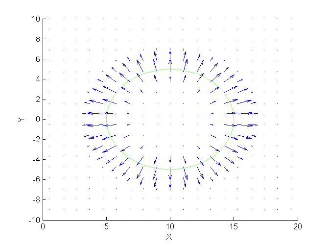
where $\tilde{\epsilon}$ represents the small floating point value returned by the eps Matlab command in order to prevent division by zero when the $(x,y)$ coordinate lies exactly on the membrane. A graph of the force using $R=5$, $L=5$, $x\in(0,20)$, $y\in(-10,10)$ and $\epsilon=\frac{R}{2}$ is shown in Figure 17. Dirichlet conditions are used in this scenario, setting $p$, $u$, and $v$ to $0$ at all of the boundaries. A contour plot shows where $z=0$ to identify the membrane.

If a spatially-constant viscosity is assumed, the decoupled system of equations from 2.13 to 2.15 can be used. Equations 2.14 and 2.15 can be simplified to provide the quickest route to the solution for $p$. An ansatz is made such that $\mathbf{u}$ is identically zero, since the membrane is circular. Under this assumption, $\Delta\mathbf{u}$ vanishes and equations 2.14 and 2.15 become

Because the fluid is stationary, the pressure is the only non-zero variable that needs to be solved. Since the membrane force acts radially outward with the magnitude depending only on $z$, it can be assumed that $p(x,y)=p(r)$. This implies converting to polar coordinates to obtain a solution. Center the polar coordinates at the center of the vesicle, and define $r$ as the distance from that center. With this definition, the signed distance from the membrane, $z$, becomes

since R is the distance from the center of the vesicle to the membrane. The gradient of a function $f$ in polar, assuming that $\frac{\partial f}{\partial\theta}=0$, is $\nabla f=f_{r}\hat{r}$. Thus, the gradient of $z$ in this coordinate system is trivial: $\nabla z=\hat{r}$. The modified Dirac Delta Function, as defined in equation 3.34, when converted to polar becomes

Thus, $\mathbf{f}$ within the region $-\epsilon+R\leq r\leq R+\epsilon$ becomes

Applying the polar gradient operator to $p$ yields $\nabla p=p_{r}\hat{r}$. Using these identities, equation 3.37 becomes

for $-\epsilon+R\leq r\leq R+\epsilon$. Equating the vector components and integrating obtains

References

- [1]
Scott, Matt (2016). Artery.jpg. Received from:
http://www.math.uwaterloo.ca/~mscott/msbioresearch.html - [2] Crowe, John H. Anhydrobiosis: An Unsolved Problem. The American Naturalist. Vol. 105, No. 946 (Nov. - Dec., 1971), pp. 563-573. Stable URL: http://www.jstor.org/stable/2459752.
- [3] Chorin, A. J. (1968). Numerical Solution of the Navier-Stokes Equations. Mathematics of Computation Vol. 22: 745–762.
- [4] Kim, Junseok. A continuous surface tension force formulation for diffuse-interface models. Journal of Computational Physics. Vol. 204 (2005) 784–804.