Blind Image Deblurring Using
Row-Column Sparse Representations

IMage blurring may come from different sources: optical defocusing, camera shaking, etc and frequently contributes to loss of captured image quality. DSLR cameras usually have image stabilizers either in the camera body or in the lenses. However, for cellphone and compact cameras, because of size limitations such mechanical stabilizers are hard to incorporate. In such scenarios, image processing algorithms are required to remove blurring artifacts in the post-processing stage. Mathematically image blurring can be well modelled as discrete convolution and image deblurring algorithms generally require solving an image deconvolution problem.

Depending on whether the Point Spread Function (PSF), aka blur kernel is known or otherwise, image deconvolution methods can be divided into two categories: non-blind image deconvolution where the PSF is exactly given and blind image deconvolution where only the blurred image is observed. The area of non-blind image deconvolution is mature with demonstrated practical success [1, 2, 3, 4, 5, 6]. Blind image deconvolution on the other hand presents a more formidable practical challenge, since the blur kernel must be automatically estimated.

Related Works: Early works in blind deconvolution include Ayers and Dainty’s work in [7] and the blind image deconvolution method based on Richardson-Lucy’s method in [8]. In [7] an iterative method similar to Wiener filter is employed in the Fourier domain, with a positivity constraint on the image, while in [8], a probabilistic solution based on Bayesian estimation is proposed.

Recent blind deconvolution methods can be divided into two groups: the first one follows an alternating minimization scheme [9, 10, 11, 12], i.e., solving for either the PSF or the image while fixing the other iteratively until convergence. The successes of these methods crucially rely on proper choices of regularizers. For instance, Shan et al. [9] employed logarithmic density of the image gradient to exploit the edge information while Krishnan et al. [10] employed a normalized sparsity measure. Xu et al. [11] employed truncated $\ell_{2}$-norm as a practical approximation of the $\ell_{0}$-norm. These methods are usually successful in recovering the latent images under relatively small motions; however, when confronted with large motions their performance may degrade due to edge distortions. Recently, Ren et al. [12] designed a weighted nuclear norm to exploit the non-local patch similarities, especially along salient edge structures. However, this method may fail to produce clear results when rich textures are present.

The second one follows a two-stage scheme [13, 14, 15], i.e., first estimating the PSF and then solving a non-blind deconvolution problem using the estimated kernel. A representative example is Fergus et. al’s method [13]. A drawback of it is the occasional ringing artifacts in the resulting images. More recent techniques [16, 11, 17] focus on dealing with large motions by pre-processing the image gradients to filter out misleading edge information. Cho and Lee [18] employed shock filter to detect salient edges, and a coarse-to-fine iterative refinement scheme to recover large kernels. Xu et al. [16] mask the edges based on a customized metric and recover the kernel using the masked edges only.

There have been notable recent breakthroughs in understanding the optimization problem involved in solving for the blur kernel and the deblurred image. Levin et al. [19] recommend estimating the kernel before the latent image instead of jointly estimating both to rule out trivial solutions. Perrone et al. in [20] verified this finding experimentally, and further found that alternating minimization over the total-variation (TV) regularized non-convex cost function can avoid converging to a trivial solution. Other works based on TV regularization include [21, 22, 23]. From a general blind deconvolution perspective (not specifically image deblurring), Ahmed et al. [24] proposed an analytical approach to convert blind deconvolution into a rank-one matrix recovery problem. Their work offers theoretical guarantees of recovery but is based on somewhat unrealistic prior knowledge about both the locations of nonzero PSF coefficients in pixel domain (blur kernel support) and the locations of primary coefficients of the image in certain transformation domains (image support).

We evaluate BD-RCS by experimenting on images taken from [36], with motion blur kernels of length from $l=7$ to $l=20$ in different directions, and a Gaussian blur kernel of radius $h=15$ and standard deviation $\sigma=1.5$ (Fig. 4) to model various realistic scenarios. Note that these PSFs are 2D, although we are using their vectorized form. The test images are included in Fig. 6 in the supplementary document, labeled Im1 – Im5. We compare against seven state-of-the-art methods for blind image deconvolution in this paper: TVBD [20], BDIRP [30], BDNSM [10], TPKE [16], HQMD [9], FBMD [17] and UNL0 [11]. For quantitative evaluations, we compute two widely-used metrics: the Signal-to-Noise Ratio (SNR) and the Improvement in Signal-to-Noise (ISNR), both in dB. ISNR is given by: $\textrm{ISNR}=10\times\mathrm{log}_{10}\left(\frac{\|\mathbf{y}-\mathbf{x}\|^{2}}{\|\mathbf{x}_{\mathrm{rec}}-\mathbf{x}\|^{2}}\right),$ where $\mathbf{y}$ is the blurry image, $\mathbf{x}$ is the original image, and $\mathbf{x}_{\mathrm{rec}}$ is the reconstructed image. We initialize the PSF with a bounding box containing all ones. We experimentally found the performance of our method robust to variations of the size of the bounding box, so long as it is conservatively selected to enclose the actual support of the blur kernel. In contrast, UNL0, BDNSM, HQMD, and BDRIP require the exact size of the kernel to produce the aforementioned results.

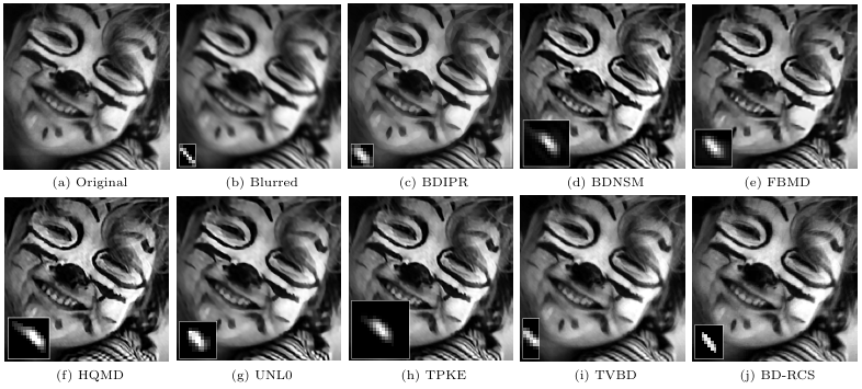
The numerical results for all the aforementioned methods are presented in Table I for motion PSFs of angle $\theta=30\degree$ and lengths $l=7,10,14$. The corresponding original, blurred, and recovered images for $l=10$ are included in the supplementary document as Fig. 11. As indicated by the numerical values, when motion gets larger, all algorithms except for TVBD [20], TPKE [16] and BD-RCS fail to plausibly recover the latent images. This fact is further supported by the visual results in the supplementary document. In particular, for kernels of length $l=10,14$, and angle $\theta=30\degree$, the recovered images for FBMD [17], UNL0 [11], BDNSM [10], HQMD [9], BDRIP [30] suffer from either blurring or ringing artifacts. The results for BDRIP [30] are typically over-smoothed as also reflected by their poor SNR and ISNR values in Table I. This can be explained by the wide supports in their reconstructed kernels. In contrast, BD-RCS achieves both the highest SNR and ISNR scores in each case, and the sharpest recovered images with the least amount of artifacts. Because only the results for TPKE and TVBD are comparable to BD-RCS for $l\geq 10$, we present results only for these methods. The numerical results are presented in Table II and one example of this case is shown in Fig. 3. Results for the remaining images are included in our supplementary document in [37].

As another challenging scenario for image deblurring we present results for an image blurred with a Gaussian kernel. This kind of blur occurs in cameras, microscopes, etc. as a result of defocussing [38]. Fig. 4 shows visual comparisons of BD-RCS against selected competing methods that are known to be generally applicable to any blur type [30, 10, 20].

In presence of more generic motion blur (as in [19]), BD-RCS cannot accurately recover the kernel while adopting Haar wavelet for building $\mathbf{C}$. Haar wavelet is not a very efficient basis for sparse coding natural images. However, BD-RCS is versatile and by adopting a customized basis (e.g. learning a dictionary to build $\mathbf{C}$), it can handle more generic blurs (both in the sense of convergence and PSF recovery, as we have no assumptions on kernel type/shape in our analysis of convergence). This is a topic for future research.

For a $256\times 256$ image the run times³³ 3 All methods (except for TPKE and HQMD that are implemented in C and hence excluded for complexity comparisons) were implemented in MATLAB on a computer with an Intel core i7-2600, 3.40 GHz CPU and 8 GB of RAM. are as follows: BDNSM: 68 sec, FMBD: 94 sec, UNL0: 296 sec, BDIPR: 300 sec, BD-RCS: 381 sec, and TVBD: 587 sec. Clearly, BD-RCS enables a more favorable performance-complexity trade-off than competing methods.

We present a novel blind image deblurring method based on structured sparse representations. Our central contribution is to develop a practical realization of a principled rank minimization framework for deconvolution by setting up practical and tractable sparsity constrained optimization problems, enabling accurate estimation of the blur kernel and image support. The proposed BD-RCS achieves a favorable cost-quality trade-off against state of the art approaches. Our work first estimates the blur kernel support followed by solving for the deblurred image. Algorithmic extensions could include performing these two steps in an alternating fashion until convergence.

Proof of Theorem 2: The basic idea is technically similar to [39], although the derivations are more involved due to the addition of $\|\mathbf{X}\|_{2,1}$. First we need the following proposition:

Also recall the dual norm of $\|{\bf X}\|_{\ast}$ is $\|\mathbf{X}\|_{2}$, i.e., the maximum singular value of $\mathbf{X}$. Using the definition of dual norm, we may reexpress $\|{\bf X}\|_{\ast}+\lambda\|{\bf X}\|_{2,1}$ as solution to the following optimization problem

and rewrite (5) as the following minimax problem:

To simplify this, let us first focus on the maximization problem:

$(P_{1})$ is equivalent to the following semi-definte programming (SDP) problem

and the following dual program

where $\overline{{\bf X}}\in{\mathbb{R}}^{2K+(K+1)N\times 2K+(K+1)N},{\bf W}_{0}\in{\mathbb{R}}^{K\times K},\{w_{i}\in{\mathbb{R}}\}_{i=1}^{K},\{{\bf V}_{i}\in{\mathbb{R}}^{N\times N}\}_{i=0}^{K}$, ${\bf I}_{k}$ is the $K\times K$ identity matrix and ${\bf e}_{i}$ denotes the $i$-th standard basis vector.

We apply the Burer-Monteiro Factorization [40] to eliminate the positive semi-definite constraint and reduce the dimensionality.

for some $r\geq\mathrm{rank}(\overline{{\bf X}})$. Equating two expressions of $\overline{{\bf X}}$ in (16) and (17) yields

Therefore, we can rewrite ${\mathrm{Tr}}(\overline{{\bf X}})$ as:

Plugging (18) and (19) back into $(P_{1})$, we get

Note the problem

has closed form solution

Then we can replace ${\bf H}_{i},i=1,2,\dots,K$ by its closed form solution in $(P_{1}^{\ast})$ to get (note $w_{i}=\|{\bf z}_{i}\|_{2}^{2}$)

Finally, since ${\bf X}={\bf Z}_{0}{\bf H}_{0}^{T}$, $\mathrm{rank}({\bf X})=\mathrm{rank}({\bf Z}_{0}{\bf H}_{0}^{T})=\mathrm{rank}({\bf Z}_{0})=\mathrm{rank}({\bf H}_{0})$, and thus we can find $\widehat{{\bf X}}$ as long as $r\geq\mathrm{rank}(\overline{{\bf X}})$.

∎

As discussed in II-C, we solve (8) using the BFGS method; for higher efficiency, we analytically derive the gradients of ${\bf Z}_{0}$ and ${\bf H}_{0}$ as follows

where $\widehat{\bm{\alpha}}=\bm{\alpha}-\sigma({\mathcal{A}}({\bf Z}_{0}{\bf H}_{0}^{T})-\widehat{{\bf y}})$, and ${\mathrm{diag}}({\bf w})$ is the diagonal matrix with its diagonal equal to ${\bf w}$. In this optimization, $\alpha$ is the Lagrange multiplier, $\sigma$ is the penalty parameter where $\sigma_{0}=1e3$, and $\rho=10$ is the scale factor. Through cross-validation [29] we observed that $r\geq 4$ yields almost identical results regardless of different image sets and initializations; therefore, we choose $r=4$. Fig. 5 presents the estimated kernels per iteration.

As we mentioned in Sec. III, we further increase the kernel length ($l\geq 15$) and included the corresponding numerical results only for TPKE, TVBD, and BD-RCS in Table II for images Im1 – Im4, respectively. The visual results for Im2 – Im4 can be found in Fig. 7 – Fig. 9, respectively. For Im4, the original image and its blurred version are included in Fig. 9a and Fig. 9b, respectively. The motion blur kernel is of $l=20,\theta=30\degree$. Fig. 9c includes the result of a well-known non-blind image deconvolution algorithm, the BM3D deblurring algorithm [2], as an approximation to the performance upper-bound for any blind image deconvolution algorithms. Fig. 9d- 9f are the recovered images from BD-RCS, TVBD and TPKE, respectively. To compare the spatial details of the images, we magnify a common part of these images and place it in the bottom right portion of each image. We also place the reconstructed blur kernel in the bottom left portion. Clearly, the TPKE algorithm usually produces ringing artifacts (Gibbs phenomenon) in the recovered images particularly around edges as it works in the Fourier domain. As for the kernel, some residuals outside the true support can be observed, although the direction appears correct. This contributes to the blurring artifacts in the recovered image; in particular, the pattern in the magnified portion is distorted. The TVBD algorithm recovers the blur kernel more accurately; however, details of the recovered image appear over-smoothed. In contrast, the BD-RCS algorithm accurately recovers both the blur kernel and the latent image, with visual quality comparable to BM3D [2]. In particular, the details in the magnified part appear almost as sharp and clear as the original image. Furthermore, the reconstructed blur kernel is also close to the original one. Indeed, their supports are exactly the same.

In this paper, we mostly focused on linear motion blur and to further corroborate the versatility of BD-RCS, we also added deblurring results for an image blurred with a Gaussian blur kernel which is represented in Fig. 4 for BD-RCS and selected competing methods that work for general type of blur kernels [30, 10, 20].

.

In the following analysis, we assume that $r$ is sufficiently large so that all the factorizations over ${\bf X}={\bf Z}{\bf H}^{T}$ are well defined; a conservative bound (depending only on $K,N,L$) for $r$ may be obtained using the methods discussed in [33], etc. We also assume $\mathcal{A}$ is an operator satisfying the following property: $\|\mathcal{A}({\bf X})\|_{2}^{2}\geq\delta\|{\bf X}\|_{F}^{2}$ for some $\delta>0,\forall~{\bf X}\in{\mathbb{R}}^{K\times N}\text{and rank}({\bf X})\leq 2r$. This property is a weaker form of the restricted isometry property (RIP) discussed in [39], and has been employed in many previous works such as [41]. We further assume that L-BFGS succeeds in finding a local minima $({\bf Z}^{k+1},{\bf H}^{k+1})$ to ${\mathcal{L}}_{\sigma_{k},{\mathcal{A}}}({\bf Z},{\bf H},{\bf w}_{k};\bm{\alpha}_{k}),~\forall~k$.

We will prove the convergence of Algorithm 1 that solves (5); proof corresponding to the algorithm solving (6) can be derived analogously. For ease of analysis (and to compensate for the scaling between (5) and (7) in the paper), we let $f^{*}$ be twice of the optimal cost of (5) in paper and let ${\bf X}^{\ast}={\bf Z^{\ast}}{\bf H^{\ast}}^{T}$ be its minimizer. We further define

We also define ${\bf w^{\ast}}$ via ${\bf w}^{\ast}_{i}=\lambda\|{\bf Z^{\ast}}{\bf H^{\ast}}^{T}\|_{2}$.

References

• [1] W. Dong, L. Zhang, G. Shi, and X. Wu, “Image deblurring and super-resolution by adaptive sparse domain selection and adaptive regularization,” IEEE Transactions on Image Processing, vol. 20, no. 7, pp. 1838–1857, July 2011.
• [2] A. Danielyan, V. Katkovnik, and K. Egiazarian, “BM3D frames and variational image deblurring,” IEEE Transactions on Image Processing, vol. 21, no. 4, pp. 1715–1728, April 2012.
• [3] J. Portilla, “Image restoration through l0 analysis-based sparse optimization in tight frames,” in IEEE ICIP, Nov 2009, pp. 3909–3912.
• [4] G. Chantas, N. P. Galatsanos, R. Molina, and A. K. Katsaggelos, “Variational bayesian image restoration with a product of spatially weighted total variation image priors,” IEEE Transactions on Image Processing, vol. 19, no. 2, pp. 351–362, Feb 2010.
• [5] J. M. Bioucas-Dias, M. A. T. Figueiredo, and J. P. Oliveira, “Total variation-based image deconvolution: a majorization-minimization approach,” in IEEE ICASSP Proceedings, May 2006, vol. 2, pp. II–II.
• [6] A. Beck and M. Teboulle, “Fast gradient-based algorithms for constrained total variation image denoising and deblurring problems,” IEEE Transactions on Image Processing, vol. 18, no. 11, pp. 2419–2434, Nov 2009.
• [7] G. R. Ayers and J. C. Dainty, “Iterative blind deconvolution method and its applications,” Opt. Lett., vol. 13, no. 7, pp. 547–549, Jul 1988.
• [8] D. A. Fish, J. G. Walker, A. M. Brinicombe, and E. R. Pike, “Blind deconvolution by means of the richardson–lucy algorithm,” J. Opt. Soc. Am. A, vol. 12, no. 1, pp. 58–65, Jan 1995.
• [9] Q. Shan, J. Jia, and A. Agarwala, “High-quality motion deblurring from a single image,” ACM Transactions on Graphics, vol. 27, no. 3, pp. 73:1–73:10, Aug. 2008.
• [10] D. Krishnan, T. Tay, and R. Fergus, “Blind deconvolution using a normalized sparsity measure,” in IEEE CVPR, June 2011, pp. 233–240.
• [11] L. Xu, S. Zheng, and J. Jia, “Unnatural l0l_{0} sparse representation for natural image deblurring,” in IEEE CVPR, June 2013, pp. 1107–1114.
• [12] W. Ren, X. Cao, J. Pan, X. Guo, W. Zuo, and M. H. Yang, “Image deblurring via enhanced low-rank prior,” IEEE Transactions on Image Processing, vol. 25, no. 7, pp. 3426–3437, July 2016.
• [13] R. Fergus, B. Singh, A. Hertzmann, S. T. Roweis, and W. T. Freeman, “Removing camera shake from a single photograph,” in ACM Transactions on Graphics, 2006, pp. 787–794.
• [14] J. Pan, Z. Hu, Z. Su, and M. H. Yang, “l0l_{0}-regularized intensity and gradient prior for deblurring text images and beyond,” IEEE Transactions on Pattern Analysis and Machine Intelligence, vol. 39, no. 2, pp. 342–355, Feb 2017.
• [15] W. Zuo, D. Ren, D. Zhang, S. Gu, and L. Zhang, “Learning iteration-wise generalized shrinkage-thresholding operators for blind deconvolution,” IEEE Transactions on Image Processing, vol. 25, no. 4, pp. 1751–1764, April 2016.
• [16] L. Xu and J. Jia, “Two-phase kernel estimation for robust motion deblurring,” in ECCV, 2010, pp. 157–170.
• [17] J. F. Cai, H. Ji, C. Liu, and Z. Shen, “Framelet-based blind motion deblurring from a single image,” IEEE Transactions on Image Processing, vol. 21, no. 2, pp. 562–572, Feb 2012.
• [18] S. Cho and S. Lee, “Fast motion deblurring,” ACM Transactions on Graphics, vol. 28, no. 5, pp. article no. 145, 2009.
• [19] A. Levin, Y. Weiss, F. Durand, and W. T. Freeman, “Understanding blind deconvolution algorithms,” IEEE Transactions on Pattern Analysis and Machine Intelligence, vol. 33, no. 12, pp. 2354–2367, Dec 2011.
• [20] D. Perrone and P. Favaro, “A clearer picture of total variation blind deconvolution,” IEEE Transactions on Pattern Analysis and Machine Intelligence, vol. 38, no. 6, pp. 1041–1055, June 2016.
• [21] M. Tofighi, O. Yorulmaz, K. Kose, D. C. Yildirim, R. Cetin-Atalay, and A. E. Cetin, “Phase and TV based convex sets for blind deconvolution of microscopic images,” IEEE Journal of Selected Topics in Signal Processing, vol. 10, no. 1, pp. 81–91, Feb 2016.
• [22] T. F. Chan and Chiu-Kwong Wong, “Total variation blind deconvolution,” IEEE Transactions on Image Processing, vol. 7, no. 3, pp. 370–375, Mar 1998.
• [23] S. D. Babacan, R. Molina, and A. K. Katsaggelos, “Variational bayesian blind deconvolution using a total variation prior,” IEEE Transactions on Image Processing, vol. 18, no. 1, pp. 12–26, Jan 2009.
• [24] A. Ahmed, B. Recht, and J. Romberg, “Blind deconvolution using convex programming,” IEEE Transactions on Information Theory, vol. 60, no. 3, pp. 1711–1732, March 2014.
• [25] “BD-RCS Webpage,” http://www.personal.psu.edu/mqt5352/BD.html.
• [26] Emmanuel J. Candès and Benjamin Recht, “Exact matrix completion via convex optimization,” Foundations of Computational mathematics, vol. 9, no. 6, pp. 717–772, 2009.
• [27] G. Liu, Z. Lin, S. Yan, J. Sun, Y. Yu, and Y. Ma, “Robust recovery of subspace structures by low-rank representation,” IEEE Transactions on Pattern Analysis and Machine Intelligence, vol. 35, no. 1, pp. 171–184, Jan 2013.
• [28] Ron Kohavi et al., “A study of cross-validation and bootstrap for accuracy estimation and model selection,” in Ijcai. Stanford, CA, 1995, vol. 14, pp. 1137–1145.
• [29] Vishal Monga, Handbook of Convex Optimization Methods in Imaging Science, Springer, 2017.
• [30] T. Michaeli and M. Irani, “Blind deblurring using internal patch recurrence,” in ECCV, 2014, pp. 783–798.
• [31] Ming Yin, Junbin Gao, Zhouchen Lin, Qinfeng Shi, and Yi Guo, “Dual Graph Regularized Latent Low-Rank Representation for Subspace Clustering,” IEEE Transactions on Image Processing, vol. 24, no. 12, pp. 4918–4933, Dec. 2015.
• [32] Ming Yin, Junbin Gao, and Zhouchen Lin, “Laplacian Regularized Low-Rank Representation and Its Applications,” IEEE Transactions on Pattern Analysis and Machine Intelligence, vol. 38, no. 3, pp. 504–517, Mar. 2016.
• [33] Samuel Burer and Renato D. C. Monteiro, “Local Minima and Convergence in Low-Rank Semidefinite Programming,” Math. Program., vol. 103, no. 3, pp. 427–444, July 2005.
• [34] Dong C. Liu and Jorge Nocedal, “On the limited memory bfgs method for large scale optimization,” Mathematical Programming, vol. 45, no. 1, pp. 503–528, Aug 1989.
• [35] “BD-RCS Convergence Analysis,” http://www.personal.psu.edu/mqt5352 /Project/convergence.pdf.
• [36] R. Köhler, M. Hirsch, B. Mohler, B. Schölkopf, and S. Harmeling, “Recording and playback of camera shake: Benchmarking blind deconvolution with a real-world database,” in ECCV, 2012, pp. 27–40.
• [37] “Supplementary document: Detailed solution of optimization problem,” http://personal.psu.edu/mqt5352/SupDoc.pdf, 2017, [Online; accessed 29-Jan-2017].
• [38] Patrizio Campisi and Karen Egiazarian, Blind image deconvolution: theory and applications, CRC press, 2016.
• [39] B. Recht, M. Fazel, and P. Parrilo, “Guaranteed Minimum-Rank Solutions of Linear Matrix Equations via Nuclear Norm Minimization,” SIAM Rev., vol. 52, no. 3, pp. 471–501, Jan. 2010.
• [40] S. Burer and R.D.C. Monteiro, “A nonlinear programming algorithm for solving semidefinite programs via low-rank factorization,” Math. Program., Ser. B, vol. 95, no. 2, pp. 329–357, 2003.
• [41] Prateek Jain, Praneeth Netrapalli, and Sujay Sanghavi, “Low-rank matrix completion using alternating minimization,” in Proceedings of the forty-fifth annual ACM symposium on Theory of computing. 2013, pp. 665–674, ACM.
• [42] Rajendra Bhatia, Matrix Analysis, vol. 169 of Graduate Texts in Mathematics, Springer New York, New York, NY, 1997.
V Solution of Optimization Using Duality