Pay for a Sliding Bloom Filter and Get Counting, Distinct Elements, and Entropy for Free
Abstract
For many networking applications, recent data is more significant than older data, motivating the need for sliding window solutions. Various capabilities, such as DDoS detection and load balancing, require insights about multiple metrics including Bloom filters, per-flow counting, count distinct and entropy estimation.
In this work, we present a unified construction that solves all the above problems in the sliding window model. Our single solution offers a better space to accuracy tradeoff than the state-of-the-art for each of these individual problems! We show this both analytically and by running multiple real Internet backbone and datacenter packet traces.
1 Introduction
Network measurements are at the core of many applications, such as load balancing, quality of service, anomaly/intrusion detection, and caching [1, 14, 17, 25, 32]. Measurement algorithms are required to cope with the throughput demands of modern links, forcing them to rely on scarcely available fast SRAM memory. However, such memory is limited in size [35], which motivates approximate solutions that conserve space.
Network algorithms often find recent data useful. For example, anomaly detection systems attempt to detect manifesting anomalies and a load balancer needs to balance the current load rather than the historical one. Hence, the sliding window model is an active research field [3, 34, 37, 41, 42].
The desired measurement types differ from one application to the other. For example, a load balancer may be interested in the heavy hitter flows [1], which are responsible for a large portion of the traffic. Additionally, anomaly detection systems often monitor the number of distinct elements [25] and entropy [38] or use Bloom filters [5]. Yet, existing algorithms usually provide just a single utility at a time, e.g., approximate set membership (Bloom filters) [6], per-flow counting [13, 18], count distinct [16, 20, 21] and entropy [38]. Therefore, as networks complexity grows, multiple measurement types may be required. However, employing multiple stand-alone solutions incurs the additive combined cost of each of them, which is inefficient in both memory and computation.
In this work, we suggest Sliding Window Approximate Measurement Protocol (SWAMP), an algorithm that bundles together four commonly used measurement types. Specifically, it approximates set membership, per flow counting, distinct elements and entropy in the sliding window model. As illustrated in Figure 1, SWAMP stores flows’ fingerprints11 1 A fingerprint is a short random string obtained by hashing an ID. in a cyclic buffer while their frequencies are maintained in a compact fingerprint hash table named TinyTable [18]. On each packet arrival, its corresponding fingerprint replaces the oldest one in the buffer. We then update the table, decrementing the departing fingerprint’s frequency and incrementing that of the arriving one. An additional counter maintains the number of distinct fingerprints in the window and is updated every time a fingerprint’s frequency is reduced to or increased to . Intuitively, the number of distinct fingerprints provides a good estimation of the number of distinct elements. Additionally, the scalar (not illustrated) maintains the fingerprints’ distribution entropy and approximates the real entropy.

1.1 Contribution
We present SWAMP, a sliding window algorithm for approximate set membership (Bloom filters), per-flow counting, distinct elements and entropy measurements. We prove that SWAMP operates in constant time and provides accuracy guarantees for each of the supported problems. Despite its versatility, SWAMP improves the state of the art for each.
For approximate set membership, SWAMP is memory succinct when the false positive rate is constant and requires up to 40% less space than [34]. SWAMP is also succinct for per-flow counting and is more accurate than [3] on real packet traces. When compared with count distinct approximation algorithms [11, 23], SWAMP asymptotically improves the query time from to a constant. It is also up to x1000 times more accurate on real packet traces. For entropy, SWAMP asymptotically improves the runtime to a constant and provides accurate estimations in practice.
| Algorithm | Space | Time | Counts |
|---|---|---|---|
| SWAMP | ✓ | ||
| SWBF [34] | ✗ | ||
| TBF [42] | ✗ |
| Problem | Estimator | Guarantee | Reference |
|---|---|---|---|
| -Approximate Set Membership | IsMember() | Corollary | |
| -Approximate Set Multiplicity | Frequency | Theorem | |
| -Approximate Count Distinct | DistinctLB | Theorem | |
| DistinctMLE | Theorem | ||
| -Entropy Estimation | Entropy | Theorem | |
the notations we use can be found in Table 3.
1.2 Paper organization
Related work on the problems covered by this work is found in Section 2. Section 3 provides formal definitions and introduces SWAMP. Section 4 describes an empirical evaluation of SWAMP and previously suggested algorithms. Section includes a formal analysis of SWAMP which is briefly summarized in Table 2. Finally, we conclude with a short discussion in Section 6.
2 Related work
2.1 Set Membership and Counting
A Bloom filter [6] is an efficient data structure that encodes an approximate set. Given an item, a Bloom filter can be queried if that item is a part of the set. An answer of ‘no’ is always correct, while an answer of ‘yes’ may be false with a certain probability. This case is called False Positive.
Plain Bloom filters do not support removals or counting and thus many algorithms fill this gap. For example, some alternatives support removals [7, 18, 19, 31, 33, 40] and others support multiplicity queries [13, 18]. Additionally, some works use aging [41] and others compute the approximate set with regard to a sliding windows [42, 34].
SWBF [34] uses a Cuckoo hash table to build a sliding Bloom filter, which is more space efficient than previously suggested Timing Bloom filters (TBF) [42].
The Cuckoo table is allocated with entries such that each entry stores a fingerprint and a time stamp. Cuckoo tables require that entries remain empty to avoid circles and this is done implicitly by treating cells containing outdated items as ‘empty’. Finally, a cleanup process is used to remove outdated items and allow timestamps to be wrapped around. A comparison of SWAMP, TBF and SWBF appears in Table 1.
2.2 Count Distinct
The number of distinct elements provides a useful indicator for anomaly detection algorithms. Accurate count distinct is impractical due to the massive scale of the data [22] and thus most approaches resort to approximate solutions [2, 12, 16].
Approximate algorithms typically use a hash function that maps ids to infinite bit strings. In practice, finite bit strings are used and bit integers suffice to reach estimations of over [22]. These algorithms look for certain observables in the hashes. For example, some algorithms [2, 26] treat the minimal observed hash value as a real number in and exploit the fact that , where is the real number of distinct items in the multi-set . Alternatively, one can seek patterns of the form [16, 22] and exploit the fact that such a pattern is encountered on average once per every unique elements.
Monitoring observables reduces the required amount of space as we only need to maintain a single one. In practice, the variance of such methods is large and hence multiple observables are maintained.
In principle, one could repeat the process and perform independent experiments but this has significant computational overheads. Instead, stochastic averaging [21] is used to mimic the effects of multiple experiments with a single hash calculation. At any case, using repetitions reduces the standard deviation by a factor of .
The state of the art count distinct algorithm is HyperLogLog (HLL) [22], which is used in multiple Google projects [28]. HLL requires bytes and its standard deviation is . SWHLL extends HLL to sliding windows [11, 23], and was used to detect attacks such as port scans [10]. SWAMP’s space requirement is proportional to and thus, it is only comparable in space to HLL when . However, when multiple functionalities are required the residual space overhead of SWAMP is only bits, which is considerably less than any standalone alternative.
2.3 Entropy Detection
Entropy is commonly used as a signal for anomaly detection [38]. Intuitively, it can be viewed as a summary of the entire traffic histogram. The benefit of entropy based approaches is that they require no exact understanding of the attack’s mechanism. Instead, such a solution assumes that a sharp change in the entropy is caused by anomalies.
2.4 Preliminaries – Compact Set Multiplicity
Our work requires a compact set multiplicity structure that support both set membership and multiplicity queries. TinyTable [18] and CQF [39] fit the description while other structures [7, 31] are naturally expendable for multiplicity queries with at the expense of additional space. We choose TinyTable [18] as its code is publicly available as open source.
TinyTable encodes fingerprints of size using bits, where is a small constant that affects update speed; when grows, TinyTable becomes faster but also consumes more space.
3 SWAMP Algorithm
3.1 Model
We consider a stream of IDs where at each step an ID is added to . The last elements in are denoted . Given an ID , the notation represents the frequency of in . Similarly, is an approximation of . For ease of reference, notations are summarized in Table 3.
| Symbol | Meaning |
|---|---|
| Sliding window size | |
| Stream. | |
| Last elements in the stream. | |
| Accuracy parameter for sets membership. | |
| Accuracy parameter for count distinct. | |
| Accuracy parameter for entropy estimation. | |
| Confidence for count distinct. | |
| Fingerprint length in bits, . | |
| Frequency of ID in . | |
| An approximation of . | |
| Number of distinct elements in . | |
| Number of distinct fingerprints. | |
| Estimation provided by DISTINCTMLE function. | |
| TinyTable’s parameter (). | |
| A pairwise independent hash function. | |
| A set of fingerprints stored in . |
3.2 Problems definitions
We start by formally defining the approximate set membership problem.
Definition 3.1.
We say that an algorithm solves the -Approximate Set Membership problem if given an ID , it returns true if and if , it returns false with probability of at least .
The above problem is solved by SWBF [34] and by Timing Bloom filter (TBF) [42]. In practice, SWAMP solves the stronger -Approximate Set Multiplicity problem, as defined below:
Definition 3.2.
We say that an algorithm solves the -Approximate Set Multiplicity problem if given an ID , it returns an estimation s.t. and with probability of at least : .
Intuitively, the -Approximate Set Multiplicity problem guarantees that we always get an over approximation of the frequency and that with probability of at least we get the exact window frequency. A simple observation shows that any algorithm that solves the -Approximate Set Multiplicity problem also solves the -Approximate Set Membership problem. Specifically, if , then implies that and we can return true. On the other hand, if , then and with probability of at least , we get: . Thus, the isMember estimator simply returns true if and false otherwise. We later show that this estimator solves the -Approximate Set Membership problem.

The goal of the -Approximate Count Distinct problem is to maintain an estimation of the number of distinct elements in . We denote their number by .
Definition 3.3.
We say that an algorithm solves the -Approximate Count Distinct problem if it returns an estimation such that and with probability : .
Intuitively, an algorithm that solves the -Approximate Count Distinct problem is able to conservatively estimate the number of distinct elements in the window and with probability of , this estimate is close to the real number of distinct elements.
The entropy of a window is defined as:
where is the number of distinct elements in the window, is the total number of packets, and is the frequency of flow . We define the window entropy estimation problem as:
Definition 3.4.
An algorithm solves the -Entropy Estimation problem, if it provides an estimator so that and .
3.3 SWAMP algorithm
We now present Sliding Window Approximate Measurement Protocol (SWAMP). SWAMP uses a single hash function (), which given an ID , generates random bits that are called its fingerprint. We note that only needs to be pairwise-independent and can thus be efficiently implemented using only space. Fingerprints are then stored in a cyclic fingerprint buffer of length that is denoted . The variable always points to the oldest entry in the buffer. Fingerprints are also stored in TinyTable [18] that provides compact encoding and multiplicity information.


The update operation replaces the oldest fingerprint in the window with that of the newly arriving item. To do so, it updates both the cyclic fingerprint buffer () and TinyTable. In CFB, the fingerprint at location is replaced with the newly arriving fingerprint. In TinyTable, we remove one occurrence of the oldest fingerprint and add the newly arriving fingerprint. The update method also updates the variable , which measures the number of distinct fingerprints in the window. is incremented every time that a new unique fingerprint is added to TinyTable, i.e., changes from to , where the method receives a fingerprint and returns its frequency as provided by TinyTable. Similarly, denote the item whose fingerprint is removed; if changes to , we decrement .
SWAMP has two methods to estimate the number of distinct flows. DistinctLB simply returns , which yields a conservative estimator of while DistinctMLE is an approximation of its Maximum Likelihood Estimator. Clearly, DistinctMLE is more accurate than DistinctLB, but its estimation error is two sided. A pseudo code is provided in Algorithm 1 and an illustration is given by Figure 1.


4 Empirical Evaluation
4.1 Overview
We evaluate SWAMP’s various functionalities, each against its known solutions. We start with the -Approximate Set Membership problem where we compare SWAMP to SWBF [34] and Timing Bloom filter (TBF) [42], which only solve -Approximate Set Membership.
For counting, we compare SWAMP to Window Compact Space Saving (WCSS) [3] that solves heavy hitters identification on a sliding window. WCSS provides a different accuracy guarantee and therefore we evaluate their empirical accuracy when both algorithms are given the same amount of space.
For the distinct elements problem, we compare SWAMP against Sliding Hyper Log Log [11, 23], denoted SWHLL, who proposed running HyperLogLog and LogLog on a sliding window. In our settings, small range correction is active and thus HyperLogLog and LogLog devolve into the same algorithm. Additionally, since we already know that small range correction is active, we can allocate only a single bit (rather than 5) to each counter. This option, denoted SWLC, slightly improves the space/accuracy ratio.
In all measurements, we use a window size of unless specified otherwise. In addition, the underlying TinyTable uses as recommended by its authors [18].
Our evaluation includes six Internet packet traces consisting of backbone routers and data center traffic. The backbone traces contain a mix of 1 billion UDP, TCP and ICMP packets collected from two major routers in Chicago [30] and San Jose [29] during the years 2013-2016. The dataset Chicago 16 refers to data collected from the Chicago router in 2016, San Jose 14 to data collected from the San Jose router in 2014, etc. The datacenter packet traces are taken from two university datacenters that consist of up to 1,000 servers [4]. These traces are denoted DC1 and DC2.
4.2 Evaluation of analytical guarantees
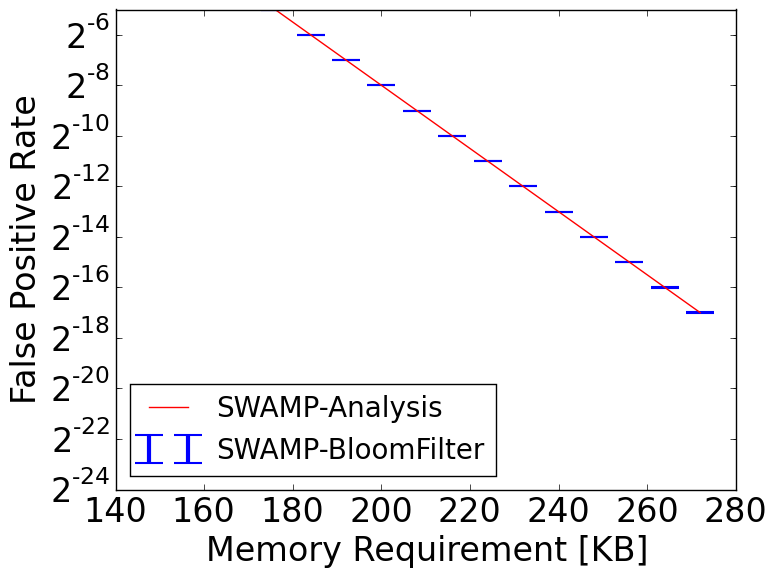
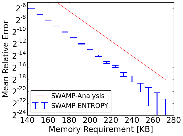
Figure 2 evaluates the accuracy of our analysis from Section on random inputs. As can be observed, the analysis of sliding Bloom filter (Figure 2(a)) and count distinct (Figure 2(b)) is accurate. For entropy (Figure 2(c)) the accuracy is better than anticipated indicating that our analysis here is just an upper bound, but the trend line is nearly identical.
4.3 Set membership on sliding windows
We now compare SWAMP to TBF [42] and SWBF [34]. Our evaluation focuses on two aspects, fixing and changing the window size (Figure 3(b)) as well as fixing the window size and changing (Figure 3(a)).
As can be observed, SWAMP is considerably more space efficient than the alternatives in both cases for a wide range of window sizes and for a wide range of error probabilities. In the tested range, it is 25-40% smaller than the best alternative.
4.4 Per-flow counting on sliding windows
Next, we evaluate SWAMP for its per-flow counting functionality. We compare SWAMP to WCSS [3] that solves heavy hitters on a sliding window. Our evaluation uses the On Arrival model, which was used to evaluate WCSS. In that model, we perform a query for each incoming packet. Then, we calculate the Root Mean Square Error. We repeated each experiment 25 times with different seeds and computed 95% confidence intervals for SWAMP. Note that WCSS is a deterministic algorithm and as such was run only once.
The results appear in Figure 4. Note that the space consumption of WCSS is proportional to and that of SWAMP to . Thus, SWAMP cannot be run for the entire range. Yet, when it is feasible, SWAMP’s error is lower on average than that of WCSS. Additionally, in many of the configurations we are able to show statistical significance to this improvement. Note that SWAMP becomes accurate with high probability using about KB of memory while WCSS requires about MB to provide the same accuracy. That is, an improvement of x27.
4.5 Count distinct on sliding windows
Next, we evaluate the count distinct functionality in terms of accuracy vs. space on the different datasets. We performed runs and summarized the averaged the results. We evaluate two functionalities: SWAMP-LB and SWAMP-MLE. SWAMP-LB corresponds to the function DistinctLB in Algorithm 1 and provides one sided estimation while SWAMP-MLE corresponds to the function DistinctMLE in Algorithm 1 and provides an unbiased estimator.
Figure 5 shows the results of this evaluation. As can be observed, SWAMP-MLE is up to x1000 more accurate than alternatives. Additionally, SWAMP-LB also out performs the alternatives for parts of the range. Note that SWAMP-LB is the only one sided estimator in this evaluation.
4.6 Entropy estimation on sliding window
Figure 6 shows results for Entropy estimation. As shown, SWAMP provides a very accurate entropy estimation in its entire operational range. Moreover, our analysis in Section is conservative and SWAMP is much more accurate in practice.
5 Analysis
This section aims to prove that RHHH solves the approximate HHH problem (Definition ) for one and two dimensional hierarchies. Toward that end, Section 5.1 proves the accuracy requirement while Section 5.2 proves coverage. Section proves that RHHH solves the approximate HHH problem as well as its memory and update complexity.
We model the update procedure of RHHH as a balls and bins experiment where there are bins and balls. Prior to each packet arrival, we place the ball in a bin that is selected uniformly at random. The first bins contain an HH update action while the next bins are void. When a ball is assigned to a bin, we either update the underlying HH algorithm with a prefix obtained from the packet’s headers or ignore the packet if the bin is void. Our first goal is to derive confidence intervals around the number of balls in a bin.
Definition 5.1.
We define to be the random variable representing the number of balls from set in bin , e.g., can be all packets that share a certain prefix, or a combination of multiple prefixes with a certain characteristic. When the set contains all packets, we use the notation .
Random variables representing the number of balls in a bin are dependent on each other.
Therefore, we cannot apply common methods to create confidence intervals.
Formally, the dependence is manifested as:
This means that the number of balls in a certain bin is determined by the number of balls in all other bins.
Our approach is to approximate the balls and bins experiment with the corresponding Poisson one. That is, analyze the Poisson case and derive confidence intervals and then use Lemma 5.1 to derive a (weaker) result for the original balls and bins case.
We now formally define the corresponding Poisson model. Let s.t. be independent Poisson random variables representing the number of balls in each bin from a set of balls . That is:
Lemma 5.1 (Corollary 5.11, page 103 of [36]).
Let be an event whose probability is either monotonically increasing or decreasing with the number of balls. If has probability in the Poisson case then has probability at most in the exact case.
5.1 Accuracy Analysis
We now tackle the accuracy requirement from Definition . That is, for every HHH prefix (), we need to prove:
In RHHH, there are two distinct origins of error. Some of the error comes from fluctuations in the number of balls per bin while the approximate HH algorithm is another source of error.
We start by quantifying the balls and bins error. Let be the Poisson variable corresponding to prefix . That is, the set contains all packets that are generalized by prefix . Recall that is the number of packets generalized by and therefore:
We need to show that with probability , is within from . Fortunately, confidence intervals for Poisson variables are a well studied [19WaysToPoisson] and we use the method of [Wmethod] that is quoted in Lemma 5.2.
Lemma 5.2.
Let be a Poisson random variable, then
where is the value that satisfies and is the density function of the normal distribution with mean and standard deviation of .
Lemma 5.2, provides us with a confidence interval for Poisson variables, and enables us to tackle the main accuracy result.
Theorem 5.1.
If then
Proof.
However, we require error of the form .
Therefore, when , we have that:
We multiply by and get:
Finally, since is monotonically increasing with the number of balls (), we apply Lemma 5.1 to conclude that
∎
To reduce clutter, we denote . Theorem 5.1 proves that the desired sample accuracy is achieved once .
It is sometimes useful to know what happens when . For this case, we have Corollary 5.1, which is easily derived from Theorem 5.1. We use the notation to define the actual sampling error after packets. Thus, it assures us that when , . It also shows that when . Another application of Corollary 5.1 is that given a measurement interval , we can derive a value for that assures correctness. For simplicity, we continue with the notion of .
Corollary 5.1.
The error of approximate HH algorithms is proportional to the number of updates. Therefore, our next step is to provide a bound on the number of updates of an arbitrary HH algorithm. Given such a bound, we configure the algorithm to compensate so that the accumulated error remains within the guarantee even if the number of updates is larger than average.
Corollary 5.2.
Consider the number of updates for a certain lattice node (). If , then
Proof.
We use Theorem 5.1 and get:
This implies that:
completing the proof.
∎
We explain now how to configure our algorithm to defend against situations in which a given approximate HH algorithm might get too many updates, a phenomenon we call over sample. Corollary 5.2 bounds the probability for such an occurrence, and hence we can slightly increase the accuracy so that in the case of an over sample, we are still within the desired limit. We use an algorithm () that solves the - Frequency Estimation problem. We define . According to Corollary 5.2, with probability , the number of sampled packets is at most By using the union bound and with probability we get:
For example, Space Saving requires counters for . If we set , we now require counters. Hereafter, we assume that the algorithm is configured to accommodate these over samples.
Theorem 5.2.
Consider an algorithm () that solves the - Frequency Estimation problem. If , then for and , solves - Frequency Estimation.
Proof.
As , we use Theorem 5.1. That is, the input solves - Frequency Estimation.
| (1) |
solves the - Frequency Estimation problem and provides us with an estimator that approximates – the number of updates for prefix . According to Corollary 5.2:
and multiplying both sides by gives us:
| (2) |
We need to prove that: . Recall that: and that is the estimated frequency of . Thus,
| (3) | ||||
where the last inequality follows from the fact that in order for the error of (3) to exceed , at least one of the events has to occur. We bound this expression using the Union bound.
An immediate observation is that Theorem 5.2 implies accuracy, as it guarantees that with probability the estimated frequency of any prefix is within of the real frequency while the accuracy requirement only requires it for prefixes that are selected as HHH.
Lemma 5.3.
If , then Algorithm satisfies the accuracy constraint for and .
Proof.
The proof follows from Theorem 5.2, as the frequency estimation of a prefix depends on a single HH algorithm. ∎
Multiple Updates
One might consider how RHHH behaves if instead of updating at most HH instance, we update independent instances. This implies that we may update the same instance more than once per packet. Such an extension is easy to do and still provides the required guarantees. Intuitively, this variant of the algorithm is what one would get if each packet is duplicated times. The following corollary shows that this makes RHHH converge times faster.
Corollary 5.3.
Consider an algorithm similar to with , but for each packet we perform independent update operations. If , then this algorithm satisfies the accuracy constraint for and .
Proof.
Observe that the new algorithm is identical to running RHHH on a stream () where each packet in is replaced by consecutive packets. Thus, Lemma 5.3 guarantees that accuracy is achieved for after packets are processed. That is, it is achieved for the original stream () after packets. ∎
5.2 Coverage Analysis
Our goal is to prove the coverage property of Definition . That is: Conditioned frequencies are calculated in a different manner for one and two dimensions. Thus, Section 5.2.1 deals with one dimension and Section with two.
We now present a common definition of the best generalized prefixes in a set.
Definition 5.2 (Best generalization).
Define as the set . Intuitively, is the set of prefixes that are best generalized by . That is, does not generalize any prefix that generalizes one of the prefixes in .
5.2.1 One Dimension
We use the following lemma for bounding the error of our conditioned count estimates.
Lemma 5.4.
([HHHMitzenmacher]) In one dimension,
Using Lemma 5.4, it is easier to establish that the conditioned frequency estimates calculated by Algorithm are conservative.
Lemma 5.5.
The conditioned frequency estimation of Algorithm is:
Proof.
Looking at Line in Algorithm , we get that:
That is, we need to verify that the return value in one dimension (Algorithm ) is . This follows naturally from that algorithm. Finally, the addition of is due to line . ∎
In deterministic settings, is a conservative estimate since and . In our case, these are only true with regard to the sampled sub-stream and the addition of is intended to compensate for the randomized process.
Our goal is to show that . That is, the conditioned frequency estimation of Algorithm is probabilistically conservative.
Theorem 5.3.
Proof.
Recall that:
We denote by the set of packets that may affect . We split into two sets: contains the packets that may positively impact and contains the packets that may negatively impact it.
We use to estimate the sample error in and to estimate the sample error in . The positive part is easy to estimate. In the negative, we do not know exactly how many bins affect the sum. However, we know for sure that there are at most . We define the random variable that indicates the number of balls included in the positive sum. We invoke Lemma 5.2 on . For the negative part, the conditioned frequency is positive so is at most . Hence, Similarly, we use Lemma 5.2 to bound the error of :
is monotonically increasing with any ball and is monotonically decreasing with any ball. Therefore, we can apply Lemma 5.1 on each of them and conclude:
∎
Theorem 5.4.
If , Algorithm solves the - Approximate HHH problem for and .
6 Discussion
In modern networks, operators are likely to require multiple measurement types. To that end, this work suggests SWAMP, a unified algorithm that monitors four common measurement metrics in constant time and compact space. Specifically, SWAMP approximates the following metrics on a sliding window: Bloom filters, per-flow counting, count distinct and entropy estimation. For all problems, we proved formal accuracy guarantees and demonstrated them on real Internet traces.
Despite being a general algorithm, SWAMP advances the state of the art for all these problems. For sliding Bloom filters, we showed that SWAMP is memory succinct for constant false positive rates and that it reduces the required space by 25%-40% compared to previous approaches [34]. In per-flow counting, our algorithm outperforms WCSS [3] – a state of the art window algorithm. When compared with approximation count distinct algorithms [11, 23], SWAMP asymptotically improves the query time from to a constant. It is also up to x1000 times more accurate on real packet traces. For the entropy estimation on a sliding window [24], SWAMP reduces the update time to a constant.
While SWAMP benefits from the compactness of TinyTable [18], most of its space reductions inherently come from using fingerprints rather than sketches. For example, all existing count distinct and entropy algorithms require space for computing a approximation. SWAMP can compute the exact answers using bits. Thus, for a small value, we get an asymptotic reduction by storing the fingerprints on any compact table.
Finally, while the formal analysis of SWAMP is mathematically involved, the actual code is short and simple to implement. This facilitates its adoption in network devices and SDN. In particular, OpenBox [9] demonstrated that sharing common measurement results across multiple network functionalities is feasible and efficient. Our work fits into this trend.
References
- [1] M. Alizadeh, T. Edsall, S. Dharmapurikar, R. Vaidyanathan, K. Chu, A. Fingerhut, V. T. Lam, F. Matus, R. Pan, N. Yadav, and G. Varghese. CONGA: Distributed Congestion-aware Load Balancing for Datacenters. In ACM SIGCOMM, 2014.
- [2] Z. Bar-Yossef, T. S. Jayram, R. Kumar, D. Sivakumar, and L. Trevisan. Counting distinct elements in a data stream. In RANDOM, 2002.
- [3] R. Ben-Basat, G. Einziger, R. Friedman, and Y. Kassner. Heavy Hitters in Streams and Sliding Windows. In IEEE INFOCOM, 2016.
- [4] T. Benson, A. Akella, and D. A. Maltz. Network traffic characteristics of data centers in the wild. In ACM IMC 2010, pages 267–280.
- [5] G. Bianchi, N. d’Heureuse, and S. Niccolini. On-demand time-decaying bloom filters for telemarketer detection. ACM SIGCOMM CCR, 2011.
- [6] B. H. Bloom. Space/time trade-offs in hash coding with allowable errors. Commun. ACM, 1970.
- [7] F. Bonomi, M. Mitzenmacher, R. Panigrahy, S. Singh, and G. Varghese. An improved construction for counting bloom filters. In ESA, 2006.
- [8] V. Braverman, R. Ostrovsky, and C. Zaniolo. Optimal sampling from sliding windows. In ACM PODS, 2009.
- [9] A. Bremler-Barr, Y. Harchol, and D. Hay. Openbox: A software-defined framework for developing, deploying, and managing network functions. In ACM SIGCOMM 2016, pages 511–524.
- [10] Y. Chabchoub, R. Chiky, and B. Dogan. How can sliding hyperloglog and ewma detect port scan attacks in ip traffic? EURASIP Journal on Information Security, 2014.
- [11] Y. Chabchoub and G. Hebrail. Sliding hyperloglog: Estimating cardinality in a data stream over a sliding window. In IEEE ICDM Workshops, 2010.
- [12] P. Chassaing and L. Gerin. Efficient estimation of the cardinality of large data sets. In DMTCS, 2006.
- [13] S. Cohen and Y. Matias. Spectral bloom filters. In Proc. of the 2003 ACM SIGMOD Int. Conf. on Management of Data, 2003.
- [14] A. R. Curtis, J. C. Mogul, J. Tourrilhes, P. Yalagandula, P. Sharma, and S. Banerjee. DevoFlow: Scaling Flow Management for High-performance Networks. In ACM SIGCOMM, 2011.
- [15] N. Duffield, C. Lund, and M. Thorup. Priority sampling for estimation of arbitrary subset sums. J. ACM, 54(6).
- [16] M. Durand and P. Flajolet. Loglog counting of large cardinalities. In ESA, 2003.
- [17] G. Einziger and R. Friedman. TinyLFU: A highly efficient cache admission policy. In Euromicro PDP, 2014.
- [18] G. Einziger and R. Friedman. Counting with TinyTable: Every Bit Counts! In ACM ICDCN, 2016.
- [19] G. Einziger and R. Friedman. Tinyset - an access efficient self adjusting bloom filter construction. IEEE/ACM Transactions on Networking, 2017.
- [20] C. Estan, G. Varghese, and M. Fisk. Bitmap algorithms for counting active flows on high speed links. In ACM IMC, 2003.
- [21] P. Flajolet and G. N. Martin. Probabilistic counting algorithms for data base applications. J. Comput. Syst. Sci., 1985.
- [22] P. Flajolet, �ric Fusy, O. Gandouet, and et al. Hyperloglog: The analysis of a near-optimal cardinality estimation algorithm. In AOFA, 2007.
- [23] E. Fusy and F. Giroire. Estimating the number of Active Flows in a Data Stream over a Sliding Window, pages 223–231. 2007.
- [24] M. Gabel, D. Keren, and A. Schuster. Anarchists, unite: Practical entropy approximation for distributed streams. In KDD, 2017.
- [25] P. Garcia-Teodoro, J. E. Diaz-Verdejo, G. Macia-Fernandez, and E. Vazquez. Anomaly-Based Network Intrusion Detection: Techniques, Systems and Challenges. Computers and Security, 2009.
- [26] F. Giroire. Order statistics and estimating cardinalities of massive data sets. Discrete Applied Mathematics, 2009.
- [27] S. Guha, A. McGregor, and S. Venkatasubramanian. Streaming and sublinear approximation of entropy and information distances. In ACM SODA, pages 733–742, 2006.
- [28] S. Heule, M. Nunkesser, and A. Hall. Hyperloglog in practice: Algorithmic engineering of a state of the art cardinality estimation algorithm. In ACM EDBT, 2013.
- [29] P. Hick. CAIDA Anonymized Internet Trace, equinix-sanjose 2013-12-19 13:00-13:05 UTC, Direction B., 2014.
- [30] P. Hick. CAIDA Anonymized Internet Trace, equinix-chicago 2016-02-18 13:00-13:05 UTC, Direction A., 2016.
- [31] N. Hua, H. C. Zhao, B. Lin, and J. Xu. Rank-indexed hashing: A compact construction of bloom filters and variants. In ICNP. IEEE, 2008.
- [32] A. Kabbani, M. Alizadeh, M. Yasuda, R. Pan, and B. Prabhakar. AF-QCN: Approximate Fairness with Quantized Congestion Notification for Multi-tenanted Data Centers. In IEEE HOTI, 2010.
- [33] J. Kubiatowicz, D. Bindel, Y. Chen, S. Czerwinski, P. Eaton, D. Geels, R. Gummadi, S. Rhea, H. Weatherspoon, W. Weimer, C. Wells, and B. Zhao. Oceanstore: An architecture for global-scale persistent storage. SIGPLAN Not., 35(11), Nov. 2000.
- [34] Y. Liu, W. Chen, and Y. Guan. Near-optimal approximate membership query over time-decaying windows. In IEEE INFOCOM, 2013.
- [35] Y. Lu, A. Montanari, B. Prabhakar, S. Dharmapurikar, and A. Kabbani. Counter braids: a novel counter architecture for per-flow measurement. In ACM SIGMETRICS, 2008.
- [36] M. Mitzenmacher and E. Upfal. Probability and Computing: Randomized Algorithms and Probabilistic Analysis. Cambridge University Press, New York, NY, USA, 2005.
- [37] M. Naor and E. Yogev. Sliding Bloom Filter. In ISAAC, 2013.
- [38] G. Nychis, V. Sekar, D. G. Andersen, H. Kim, and H. Zhang. An empirical evaluation of entropy-based traffic anomaly detection. In ACM IMC, 2008.
- [39] P. Pandey, M. A. Bender, R. Johnson, and R. Patro. A general-purpose counting filter: Making every bit count. In ACM SIGMOD, 2017.
- [40] O. Rottenstreich, Y. Kanizo, and I. Keslassy. The variable-increment counting bloom filter. In INFOCOM, 2012.
- [41] M. Yoon. Aging bloom filter with two active buffers for dynamic sets. IEEE Trans. on Knowl. and Data Eng., 2010.
- [42] L. Zhang and Y. Guan. Detecting click fraud in pay-per-click streams of online advertising networks. In ICDCS, 2008.