Levitation of non-magnetizable droplet inside ferrofluid
Abstract
The central theme of this work is that a stable levitation of a denser non-magnetizable liquid droplet, against gravity, inside a relatively lighter ferrofluid – a system barely considered in ferrohydrodynamics – is possible, and exhibits unique interfacial features; the stability of the levitation trajectory, however, is subject to an appropriate magnetic field modulation. We explore the shapes and the temporal dynamics of a plane non-magnetizable droplet levitating inside ferrofluid against gravity due to a spatially complex, but systematically generated, magnetic field in two dimensions. The coupled set of Maxwell’s magnetostatic equations and the flow dynamic equations is integrated computationally, utilizing a conservative finite-volume based second order pressure projection algorithm combined with the front-tracking algorithm for the advection of the interface of the droplet. The dynamics of the droplet is studied under both the constant ferrofluid magnetic permeability assumption as well as for more realistic field dependent permeability described by the Langevin’s non-linear magnetization model. Due to the non-homogeneous nature of the magnetic field, unique shapes of the droplet during its levitation, and at its steady state, are realized. The complete spatio-temporal response of the droplet is a function of the Laplace number , the magnetic Laplace number , and the Galilei number ; through detailed simulations we separate out individual roles played by these non-dimensional parameters. The effect of the viscosity ratio, the stability of the levitation path and the possibility of existence of multiple-stable equilibrium states is investigated. We find, for certain conditions on the viscosity ratio, that there can be developments of cusps and singularities at the droplet surface; this phenomenon we also observe experimentally and compare with the simulations. Our simulations closely replicate the singular projection on the surface of the levitating droplet. Finally, we present an dynamical model for the vertical trajectory of the droplet. This model reveals a condition for the onset of levitation and the relation for the equilibrium levitation height. The linearization of the model around the steady state captures that the nature of the equilibrium point goes under a transition from being a spiral to a node depending upon the control parameters, which essentially means that the temporal route to the equilibrium can be either monotonic or undulating. The analytical model for the droplet trajectory is in close agreement with the detailed simulations.
keywords
Droplet levitation, ferrofluid.1 Introduction
The buoyancy due to the gravitational field is the oldest known mechanism of levitation of matter inside fluids. It is only the past few decades that the researchers have used other gravity compensation techniques for levitating objects in liquids or gases. For example using acoustics (Trinh, 1985), optical technique by utilizing photon momentum transfer (Price et al., 2015), using magnetic fields to levitate objects inside paramagnetic substances (Ikezoe et al., 1998), inside magnetic nanofluids (Rosensweig, 1966), inside air (Geim et al., 1999), and more recently studying the effect of lasers (Limbach et al., 2016).
In the context of magnetic nanofluids or ferrofluids11 1 Ferrofluid is a colloidal suspension of surfactant coated magnetic nanoparticles (characteristic size nm) inside a suitable carrier liquid (Rosensweig, 1985)., one of the earliest observation of solid levitation inside ferrofluid was made by Rosensweig (1966). It was observed that a solid magnet dispersed inside a ferrofluid levitates itself against the gravity. Thereafter, the levitation of solid objects inside ferrofluids has found numerous technological and research applications in recent years. The principle has been investigated for non-magnetic solid particle separation from a continuous stream of ferrofluid (Pamme, 2006; Vojtíšek et al., 2012). In a similar manner, it has also been used in biological cell sorting at micro-scale utilizing a magnetic fluid as the outer phase liquid (Zhu, 2013). The transport of diamagnetic particles is another application (Dunne et al., 2007; Liu et al., 2014; Zhu et al., 2011b). As sometimes required in biology, the gravity compensating environment can also be achieved through the levitation of non-magnetizable objects inside ferrofluids (Beysens & van Loon, 2015). For example, the research has shown that the magnetically created microgravity environment through magnetic levitation is technically applicable in the control of crystallization (Huber & Littke, 1996). Recently, the magnetic levitation has been successfully utilized to measure the density of solid and immiscible liquids (Mirica et al., 2009). As the magnetic fields can be generated using electromagnets integrable to electronics, the process has a tremendous potential for smart sensor applications. Such efforts have already been made, for example the development of magnetic actuators (Olaru et al., 2013).
Though the experimental evidence of solid phase levitation inside ferrofluid came right after the invention of ferrofluids, very little efforts have been made till date to investigate the same for a liquid phase levitation. A distinct hydrodynamics is certainly expected in the latter case due to the presence of a deformable liquid-liquid interface instead of a rigid liquid-solid interface. It is physically tempting to study this system and to look for, if any, the distinguishing behaviors. Similar to the practical applications of solid object levitation inside a ferrofluid, the liquid phase levitation might also have useful applications, especially in the modern small scale devices.
Many of the facets of the interface between a magnetizable and a non-magnetizable liquid are exhibited by the ferrofluid droplets. Numerous intriguing features of the ferrofluid interfacial phenomena, such as deformations, appearance of peculiar shapes, small scale instabilities at the interface, wetting, hysteresis, merging and break-up, stretching and pinning, and many more can be fundamentally studied using the droplet systems. The motivation also comes from looking at the in-use and future possible applications of ferrofluid droplets such as micro scale mixing (Mugele et al., 2006), inkjet-printing (Verkouteren & Verkouteren, 2011), transport of surfactant (Wojciechowski & Kucharek, 2009; Kovalchuk & Vollhardt, 2001), transport of drugs in biological systems, vibrating interfaces (Kim & Lim, 2015; Whitehill et al., 2011) and so on.
The investigations focusing ferrofluid droplets seem to start accelerating from , although seminal works had been already performed on relevant droplet systems, e.g. by Taylor (1964) on the disintegration of water droplets due to electric field and Rosenkilde (1969) on dielectric droplet in an electric field. Bacri & Salin (1983) found that magnetic field over a threshold value can destabilize a ferrofluid droplet. The researchers found that the shape of the ferrofluid droplet can change from an elongated one to a slender one. They used anionic ferrofluid in their experiments to get high agglomerate concentrations to achieve this transition regime. Sherwood (1988) studied the breakup dynamics of droplets from a more general point of view as he investigated the effect of both electric and magnetic field. A more rigorous analysis of the equilibrium shapes of the ferrofluid droplet seems to be first performed by Sero-Guillaume et al. (1992). The researchers used an energy minimization principle and studied both partially and totally free ferrofluid droplets. They found interesting bifurcating solutions and hysteresis mechanisms. Wohlhuter & Basaran (1993) investigated polarizable drops and their stability in external fields. Near the same time, Bacri et al. (1994) reported, for the first time, the magnetic fluid micro droplet behavior under a rotating magnetic field. A starfish like shape instability was observed by the investigators. Later Sandre et al. (1999) studied the behavior of highly magnetic droplet under rotating and modulated fields. They observed the rotations of the droplet to be synchronous with the applied field and also the breakup of the droplet at increased vorticity. Recently, the researchers have shown interest in the ferrofluid droplet patterns (Jackson, 2005; Timonen et al., 2013), formation processes (Chen & Li, 2010; Liu et al., 2011a; Liu et al., 2011b) and instabilities at its interface (Bashtovoi et al., 1999; Chen & Cheng, 2008).
In the last decade and near the start of the present one, efforts have been made to investigate the deformation dynamics, motion and manipulation of the ferrofluid droplets under different field configurations and using different tools such as numerical programs (Afkhami et al., 2008; Afkhami et al., 2010), image processing (Koh et al., 2013) and other experimental techniques (Nguyen, 2013). Jackson & Miranda (2007) observed unique regular and irregular ferrofluid droplet shapes inside a Hele-Shaw cell under cross magnetic fields applied normal to the cell plane. Afkhami et al. (2008) investigated the motion of a ferrofluid droplet through a viscous medium and subsequently (Afkhami et al., 2010) did a numerical and experimental study to predict its deformation and shape. Chen & Cheng (2008) experimentally studied the Rosensweig instability of a ferrofluid droplet. Zhu et al. (2011a) simulated the experimentally observed droplet shapes and found its deformation to be non-linearly related to the magnetic Bond number. From microfluidic application point of view, Wu et al. (2013) investigated the formation and breakup of a ferrofluid droplet in a microfluidic flow focusing device. Before that, Tan et al. (2010) studied similar aspects in a microfluidic T-junction. New applications have also emerged in recent for example energy harvesting using ferrofluid droplets (Kim et al., 2015; Kim & Yun, 2015), micro structure printing (Fattah et al., 2016) and optofluidic devices (Gu et al., 2015). Recently in an experimental work, Gu et al. (2016) have observed the non-linear behavior of a ferrofluid droplet under the application of a periodic field. Lira & Miranda (2016) found a very interesting family of stable polygonal shapes of ferrofluid droplet for quasi-two dimensional conditions using a vortex-sheet formulation. Most recently Rowghanian et al. (2016) have obtained further important insights into the ferrofluid deformation dynamics.
It is notable that though a decent amount of research has been conducted on the ferrofluid droplet behavior inside non-magnetizable environment, the inverse system has not been explored up to its fundamental dynamical and interfacial details. Relevant exceptions are the studies by Duplat & Mailfert (2013), where the researchers have studied a bubble shape in magnetically compensated gravity environment inside liquid oxygen, by Ueno et al. (1995); Ueno et al. (1999) and Korlie et al. (2008) for bubbles in simplified uniform field conditions. Again a heavy settled droplet rise against the gravity in a non-uniform field condition is not tackled. Though globally the droplet will respond along the applied field gradient in the inverse system (repel away from the magnetic source), the difference lies in the fact, as will be shown in our study, that the local flipping of the direction between the curvature and the magnetic force at the interface in the inverse system can cause intriguing interplay between the magnetism and the fluid flow, especially under the non-uniformity of the magnetic field, and results in unique droplet shapes and its interfacial features. Furthermore, the inverse system is technically equally relevant to the droplet manipulation technologies, creating gravity compensation environments for the small scale droplets, and in sensing applications based on such principles, though it has not received due attention.
In free space, it is well known that a stable levitation of a permanent magnet is proven to be not possible by the Earnshaw’s theorem — a consequence of the fact that the Maxwell’s equations do not permit a magnetic field maximum in free space (Geim et al., 1999). Although the opposite is possible for a diamagnetic substance, which requires a filed minimum rather than a maximum. However, if the surrounding medium is not a free space and is fluid, and at the same time, is itself magnetizable, the situation is then different for a dispersed diamagnetic substance. In addition this system even permits for the levitation of a non-magnetic object.
In this work, the temporal dynamics and the spatial shapes of a plane non-magnetizable liquid droplet levitating inside a ferrofluid against gravity due to a spatially complex, but systematically generated, magnetic field have been studied in a two dimensional environment, primarily through numerical computations. The coupled Maxwell’s magnetostatic equations and the flow dynamic equations are integrated computationally, utilizing a finite-volume based conservative second order pressure projection algorithm combined with the front-tracking algorithm for the advection of the interface of the droplet. To support our simulations, we demonstrate the non-magnetizable droplet levitation experimentally and compare the interfacial singular projections obtained from the simulations with the experimental observations. Finally, we present a non-linear analytical model for the droplet trajectory in the vertical direction.
The mathematical formulation of the problem, and the physical basis for it, is presented in §2 and §3 while the numerical solution methodology is described in §4. The discussion and analysis of the levitation phenomenon is broken into several parts — §5 describes basic characteristics of the droplet shape, time-dependent levitation height, and the effect of non-dimensional parameters on the same; the effects due to viscosity ratio between the two phases are explored in §6; the effects of the non-linear magnetization of the ferrofluid are presented in §7. We study the stability conditions for the levitation path and the final equilibrium location in §8 and compare the experimentally observed phenomenon with the simulation in §9. In §10, we describe the analytical model for the levitation height, the necessary condition for the onset of the levitation as well as the transitions in the solution behavior near the equilibrium levitation point. Finally we summarize our findings in §11.
2 Phenomenon
2.1 Setup and visualization


To lay down the physical basis for the numerical computations, first we experimentally demonstrate the phenomenon of a non-magnetizable droplet levitation inside a ferrofluid. This approach has actually helped us to first understand about a realistic set of magnetic field boundary conditions that can lead to a stable levitation of the droplet.
The levitation of the droplet is visualized in a Hele-Shaw cell arrangement. The cell is made up of two closely spaced transparent poly-methyl-methacrylate (PMMA) sheets of size , shown in figure 1 (left). The figure shows the PMMA sheets prior to the manufacture of the cell. The four sides of the cell are closed by inserting a thin polymer sheet cuttings in between the PMMA sheets. The final effective volume of the cell is measured to be .
The cell is filled with a sample of kerosene based ferrofluid (a precise description of the magnetic characterization of the ferrofluid sample, apparatus and image analysis is given later in §9 while comparing with the simulations). A small droplet of water with volume is placed into the cell before its closure, where is the droplet radius and is the gap between the walls of the Hele-Shaw cell. The size of the droplet is predicted using image processing after it is dispensed into the cell (). The plane of the cell is kept parallel to the direction of the gravity, and thus in the absence of the field, the droplet remains settled at the bottom.
The levitation against the gravity is now initiated by placing the cell on the surface of a permanent magnet; the magnets used are of Neodymium and a pair is shown in figure 1 (left) together with the cell. Figure 1 shows the phenomenon recorded during one of the experiments under the above stated conditions. Seven different time instants during the evolution of the droplet are shown in the figure. Initially, the droplet rests on the bottom wall. After the application of the field at the bottom of the cell, the droplet begins to levitate and the shape of the droplet alters – it elongates laterally and attains a concavity at the bottom. Eventually it attains almost an elliptic shape.
2.2 Stable levitation

Under the influence of a single magnet at the base, it is noticed that the location of the levitated droplet is not exactly stable; there is a side wise movement of the droplet in addition to its vertical rise and the levitation path is not exactly a straight trajectory. In other words a stable levitation is not achieved using a single magnet at the bottom; after some initial period the droplet path tilts towards the side walls. To achieve a stable levitation and to restrict the side wise drift of the droplet, an additional pair of neodymium magnets, one at each side wall of the cell, is attached to provide a force on the droplet directing from the side walls towards the center of the cell. The single magnet at the bottom is now also replaced with a pair so that the north and south ends of the magnets make contact to each other in alternative fashion and thus remain attached to the cell. That is, if the north pole of a magnet is in contact with the wall, then its adjacent magnets will have their south poles in contact with the respective walls — an arrangement very similar to the Halbach array of magnets (Halbach, 1985). One pair of magnets at the top wall closes the loop. The presence of this complimentary pair at the top wall is expected to reduce the levitation height of the droplet, but its absence gives rise to a field configuration which affect the stability of the levitation negatively and in an interesting way (here briefly, the absence of this pair of magnets at the upper wall gives rise to more than two possible equilibrium locations for the droplet; we elaborate on it in §8). In figure 1 (left), one such pair of magnets is shown. The complete schematic for the magnet arrangement is shown in figure 3, and is further explained below in section 3.
One of the experimental demonstration conducted with this arrangement of magnets is shown in figure 2. Eight different time instants are shown in the figure. Initially the water droplet remains in the vicinity of the bottom wall. Under this arrangement of magnets, the droplet eventually finds an stable equilibrium position depending upon the balance between the gravitational, buoyancy and the magnetic forces. Certainly, other magnet arrangements for a stable levitation of the water droplet may also be possible; the current alternating arrangement has proven specifically helpful in incorporating the magnetic field boundary conditions conveniently in terms of sine functions multiplied by the maximum strength of the magnet (§3.2). This Halbach array arrangement is also practically helpful in keeping the magnet edges in contact with each other without any external forcing.
2.3 Physical explanation
A possible physical explanation of the phenomena can be given after Rosensweig (1985). First let us assume that there is no droplet. When the cell is brought in contact with the magnet, and then held stationary, the ferrofluid is attracted towards the magnet. For an initial period of time, some transients appear inside the ferrofluid due to this attractive force. However, as the cell is then kept stationary and there is not a continuous supply of work, the stationary magnetic force cannot make the ferrofluid to move continuously due to the thermodynamic constraints. The stresses inside the ferrofluid reorient themselves to counter this perpetual motion, much like the pressure redistribution in the gravitational field. The net response from the ferrofluid in this static condition is the redistribution of the mechanical pressure to balance the magnetic and gravitational forces; the pressure being higher in higher magnetic field regions. Now if a non-magnetizable object is placed inside the ferrofluid, it experiences the developed pressure gradient and starts moving away from the magnet. In the next section we describe the mathematical basis of our computations.
3 Mathematical formulation
The kerosene based ferrofluid-water combination inside the cell in our experiments represents an immiscible, incompressible two-phase system in two dimensions. We mimic this flow environment inside the cell by considering a square domain . The domain consists of two fluid phases. The ferrofluid makes the bulk phase , while a non-magnetizable droplet of an immiscible liquid is considered inside it (figure 3). The cell is covered with four magnet pairs in a Halbach array arrangement, as shown. The bottom pair of magnets initially remains detached from the cell and the droplet remains settled at the bottom. The levitation is initiated when this pair is brought in contact to the bottom wall. In other words, both the fluid phases initially remain quiescent under the gravity and the magnetic field (applied at the top and the side walls). The flow is then initiated at some time instant (marked as ) when the magnetic field is applied at the bottom wall. For computational simplicity, we utilize a two-dimensional idealization of the actual cell in our simulations. Considering the fact that the PPMA sheets were coated against the adhesion of the liquids, any effect arising due to the contact line pinning with the parallel walls are neglected. We also neglect the effects of the interfacial curvature along the third dimension perpendicular to the plane of the cell. Though, in general this can have an effect on the stability of the interface, we shall show, while comparing the simulations in section §9, that these idealized simplifications have not introduced any considerable and qualitative change in the dynamics and geometry of the droplet interface during its rise.
3.1 Dimensional form of the governing equations
The motion of the non-magnetic droplet inside ferrofluid medium, and the continuous local flow and the magnetic field, are described by a coupling between the Navier-Stokes equations and the Maxwell’s equations of electromagnetism. If the fluids are considered electrically non-conducting, and assuming that the relaxation time of the magnetic nano-particles in the ferrofluid is much smaller than the relevant hydrodynamic time scales, the Maxwell’s equations reduce to the magnetostatic form,
| (1) |
where , and are the magnetic flux density, the magnetic field and the magnetization respectively while is the free space magnetic permeability. The irrotationality of permits the relation
| (2) |
where is a scalar magnetic potential. Also is constitutively related to through
| (3) |
where is the magnetic susceptibility. For ferrofluids in general, the magnetization is itself governed by a differential equation involving magnetization relaxation time, however here we assume that the relaxation time is small and the magnetization relaxes in infinitesimally small time, so called quasi-equilibrium ferrohydrodynamic hypothesis. A single scalar equation can be obtained using equation 2 and 3 in equation 1, expressed as
| (4) |
where the quantity is equal to the magnetic permeability.
The ferrofluid susceptibility varies with the magnetic field strength and other thermodynamic variables. In this study we consider it either a constant or a function of the local magnetic field. The simplifying assumption of constant permeability of ferrofluid is used in the first two set of simulations to obtain the basic characteristics of the droplet shape and levitation height, while being computationally efficient. It has also served as a reference for further refinement of our simulations using a more realistic field-dependent permeability model, when the experimentally observed shape is compared with the simulations. In the latter case, the magnetization relation 3 can be written in its non-linear form, i.e. . Then the equation for magnetic potential is different for and and is expressed as (using Langevin’s non-linear magnetization equation)
| (5) |
where is the saturation magnetization of ferrofluid and . It should be noted that this specific non-linear ferrofluid magnetization model assumes that the ferrofluid exhibits nearly a paramagnetic behavior and also does not reflect the hysteresis of magnetization. It further assumes nearly mono-disperse size distribution of the magnetic nano-particles and negligible dipole-dipole interactions. For non-magnetic liquids, the magnetic susceptibility is usually negligible, or in other words, their permeability can be considered equal to the free space permeability . The equation 5 serves as the key to obtain over the whole domain .
The equations for the isothermal and incompressible flow field are
| (6) |
where and are the mechanical pressure, viscous stress tensor, magnetic stress tensor, gravitational acceleration and the interfacial force respectively. The Newtonian viscous stress tensor is . The force is expressed as and acts singularly at the interface. Here is the local curvature of the interface, is the unit outward normal at the interface and is the delta function at the interface.
The driving force in the present study is due to the magnetic stresses. There are number of different expressions for that exist in the ferrohydrodynamic literature; interestingly, under incompressible and isothermal conditions and for isotropic permeability , the existing expressions for magnetic stress tensor reduce to the form
| (7) |
where the first part , which contains the isotropic magnetic pressure, can safely be lumped with (Rosensweig, 1985; Afkhami et al., 2008). This form of the magnetic stress tensor is particularly well adaptable to a conservative finite-volume formulation in comparison to the magnetic body force density expressions such as the Kelvin force density or the Korteweg-Helmholtz force density which are derivable by taking the divergence of . We directly discretize the divergence of 7 on finite volume cells utilizing (where and denote the computation cell volume, cell surface and the outward normal at the cell surface respectively), which conserves the magnetic force fluxes for each individual computational cell.
3.2 Initial, boundary and interfacial conditions
The no-slip and the no-penetration flow boundary conditions are considered at all the four walls while sinusoidal boundary conditions are considered for the gradient of magnetic potential to replicate the Halbach array of magnets, described as
| (8) |
where is the unit normal at the walls pointing into and subscripts and represent top, left, right and bottom wall respectively.
Although the conditions at the interface are not explicitly needed in the numerical treatment of the two-phase, one-fluid formulation (Tryggvason et al., 2011), we state them below for the sake of completeness. At the interface, the normal component of the magnetic flux density, the tangential component of the magnetic field, the tangential component of the total stress, and the velocity are continuous, while there is discontinuity in the normal component of the total stress,
| (9) |
where is the total stress tensor and denotes the difference of a quantity, , right across the interface.
3.3 Non-dimensionalization
Looking at the governing model, the flow solution can be considered as dependent on the following dimensional parameters
| (10) |
The number of independent variables are reduced by properly identifying the non-dimensional groups which influence the flow solution. Taking as the reference for all the properties except the magnetic permeability, for which FF has the permeability higher than the droplet medium, and considering the following reference scales,
| (11) |
the equations of fluid motion are normalized to the following form
| (12) |
where the non-dimensional group
| (13) |
is the Laplace number signifying the ratio of the interfacial force to the the viscous force,
| (14) |
is the magnetic Laplace number signifying the ratio of the magnetic force to the the viscous force, and
| (15) |
is the Galilei number signifying the ratio of the gravitational force to the viscous force.
The Maxwell’s equations transform to the following non-dimensional form,
| (16) |
where . The magnetization relation takes the following normalized form
| (17) |
where
| (18) |
Using this relation for magnetization, the equation for magnetic potential takes the following non-dimensional form
| (19) |
or
| (20) |
Therefore, four non-dimensional parameters, and are significant and thus the flow solution in case of field dependent ferrofluid susceptibility can be expressed by the functional form
| (21) |
In case of constant ferrofluid susceptibility, where there is no bound on , the reference scale for the magnetization is chosen equal to . In such case the functional form of the flow solution reads
| (22) |
The parameter depicts the effect of non-linearity of the magnetization on the flow solution. In the following sections we drop out the star symbols on the non-dimensional variables for convenience.
4 Numerical method
We solve the flow dynamic equations 6 numerically utilizing the one-fluid approach (Tryggvason et al., 2011) in which the set of equations over the whole domain can be solved if the spatial distributions of the fluid properties are known. We perform the space discretizations of the flow dynamic equations 6 as well as the magnetic potential equation 5 using the finite volume method over a standard staggered rectangular grid. To march in time, we utilize a second order pressure projection algorithm. The two phases are recognized using a marker function
| (23) |
To advect the marker function, we use the front-tracking scheme of Unverdi & Tryggvason (1992), in which the interface location is first updated using the velocity field solution and then the marker function is reconstructed from the known interface location. The detailed description of the projection algorithm, the front-tracking algorithm and the principles of finite-volume discretization are presented in Tryggvason et al. (2011), and here we only describe the incorporation of equation for magnetic potential (4), the handling of the magnetic permeability field and the incorporation of the magnetic stresses in the equation of motion 6 in the overall algorithm.
| Phase | ||||||
|---|---|---|---|---|---|---|
| Ferrofluid () | ∗ | 57.7 | ||||
| Water () | - | 0.0 |
∗Computed using Langevin’s function for ferrofluid magnetization.
4.1 Description of the algorithm
Initially at , both the fluids are considered quiescent . The initial location of the interface between the two phases is considered to be known, or in other words, the initial discrete distribution of the fluid property fields - - on the grid is considered to be known; being the indices associated with concerned grid point. Knowing at , the equation for the magnetic potential (4) is first solved. Obtaining , is obtained from . Once is known, the magnetic body force is computed. The equation of motion 6 is then solved for the velocity field using the pressure projection algorithm (Tryggvason et al., 2011). Using , the location of the interface is then advected, and from this updated location of the interface, the discrete marker function is reconstructed using the front-tracking algorithm (Tryggvason et al., 2011; Unverdi & Tryggvason, 1992). The discrete density and viscosity fields are then interpolated from as
| (24) |
The permeability is obtained in a similar fashion if it is assumed constant in both the phases. However, when the non-linear magnetization model is considered, the permeability is considered constant only in the non-magnetizable phase. In the magnetizable phase, it is predicted using the Langevin’s relation for the ferroflud magnetization. Both the above cases are summarized as
| (25) |
Once the property fields are advected, the algorithm is advanced to the next time step and the numerical cycle is repeated till desired time.
The use of constant magnetic permeability is a greater computationally simplification and results in lower computational times. Therefore it is useful for obtaining very basic features of the flow, and also when parameters other than magnetic permeability (or susceptibility) were varied. An example is the variation of viscosity ratio, which is not related to the permeability or magnetization of the ferrofluid in our formulation. However, instead of varying the permeability ratio, and for comparison with experiments, we adopt the non-linear magnetization model.
The spatial as well as the temporal discretizations in our scheme are second order accurate. The advection term in the momentum equation is handled using a second order essentially non-oscillatory (ENO) scheme while the standard second order centered in space discretization is applied to the diffusive viscous terms. The interpolations of the viscosity at the computational cell faces are performed harmonically while the density and the permeability are interpolated arithmetically. A highly optimized V-cycle MULTIGRID method is implemented for the solution of the pressure Poisson equation and the equation for the magnetic potential.
4.2 Setup of simulations
| Section | §5 | §6 | §7 | §8 | §9 | ||||||||||
|---|---|---|---|---|---|---|---|---|---|---|---|---|---|---|---|
| Focus |
|
|
|
|
| ||||||||||
| 0.1,1.0,10.0 | 0.1,1.0,10.0 | 0.1 | 10.0 | 2.09 | |||||||||||
| 40,160,360,640,1000 | 40,160,360,640,1000 | 1000∗ | 360,1000 | 5862.79∗ | |||||||||||
| 0.1,1.0,10.0 | 0.1,1.0,10.0 | 0.1 | 1.0 | 38.6 | |||||||||||
| 2 | 2 | 2 | 2 | 1.152 | |||||||||||
| 2 | 0.5 | 2 | 2 | 0.04 | |||||||||||
| 0.25 | 0.25 | ∗∗ | 0.25 | ∗∗ | |||||||||||
| ∗∗∗ | ∗∗∗ |
|
∗∗∗ | 2.06 |
.
∗The vacuum permeability is used to compute characteristic , as the permeability of the ferrofluid in this case is a variable determined by Langevin’s function.
∗∗The quantity is computed using Langevin’s function for the field dependent ferrfluid magnetization.
∗∗∗The quantity is not uniquely defined, or do not appears in the formulation.
The properties of the two fluids are presented in table 1, where , and . We consider a water droplet of radius of . The magnetic fields used in our experiments are of while the order of permeability of ferrofluid is considered a multiple of . For these orders of magnitude of the properties, the and can be as high as , while a realistic turns out to be . Considering these, we simulate for and in the range while for in the range . Being conservative, the is not increased further to avoid any numerical instability arising due to the higher order of the magnetic source term in the momentum equation.
The value of the parameter changes due to change in , as or do not vary for a given ferrofluid sample. Here, the initial susceptibility of ferrofluids is measured to be , while . Thus for applied field between , the order of is expected to vary between . We simulate for in the range .
The breakup of simulations and all the corresponding simulation parameters are summarized in table 2. The simulations are divided into six different sets with different foci. In the first set, we simulate for constant permeability in both the phases. Next, the effect of viscosity ratio is investigated. In the third set of simulations, the effects of field dependent ferrofluid permeability, or equivalently the effects of non-linear magnetization, are simulated. The stability of levitation is the focus of the subsequent set, while the appearance of interfacial singularity and comparison with experiment is addressed through the last set of simulations. The same hierarchy, as listed in table 2, is utilized for sectioning the results.
4.3 Output fields and variables
Besides the magnetic and velocity field solutions, we study the shapes of the levitating droplet, the final levitation height, the time dependent displacement and velocity of the droplet tip/nose, the droplet deformation (defined below), and the time averaged change in the droplet deformation. In certain cases, we also utilize the absolute magnetic field contours and the vorticity contours.
The discrete information about the interface is described by two vectors - and - storing and co-ordinates of discrete interface points. This structure is compatible with the implementation of front-tracking algorithm. The total number of interface points , however, can be different for each time step due to their dynamic addition or deletion, a part of the front-tracking algorithm. From this information about the interface, the vertical distance of the tip of the droplet from the bottom wall is extracted using
| (26) |
and the speed of the tip is computed using
| (27) |
where is the time step.
To study the time dependent deformation of the levitating droplet, a global droplet deformation parameter or shape factor, , is computed from the interface information using
| (28) |
Notice that can be negative if , which implies that the vertical span of the droplet is more than its horizontal span.
To show the complete curve for all the simulations is a cumbersome task. To mark the average extent of the droplet deformation over all times, a time averaged shape factor, , is computed. It reduces the results for the shape factor to one value for one simulation. The expression for is
| (29) |
where is the time up to which the flow is simulated.
4.4 Code Validation and Grid and time step independence
The computational code is developed and tested for single phase as well as two phase viscous incompressible flow, with and without the magnetic effects, and has been successfully applied in problems by the authors to predict the interfacial (Singh et al., 2016b) and relaxation mechanisms (Singh et al., 2016a) in ferrofluids. We incorporate the non-linear magnetization/field dependent permeability model and the conservative discretization of the full magnetic body stress tensor, and a highly optimized multigrid technique for the solution of the pressure Poisson and the magnetic potential equation. For the problem at hand, the grid as well as the time step independence of the code is carefully studied. The details of these consistency checks have been presented in appendix A. Besides these quantitative consistency checks, the physical correctness also confirmed in our study through its ability to predict the experiments, especially the fine features at the interface (§9).
5 Droplet shapes and levitation height: Effect of and
In the first set of simulations, the magnetic permeabilities () are considered constant. As discussed before, this theoretical assumption served as a reference for further refining of our simulations using a more realistic field-dependent permeability model. The simulation parameters are given in the second column of table 2. The intermediate case of and – respectively and – is first discussed, while the variations in and are discussed afterwards.
The numerically predicted movement of the droplet for the above values of the non-dimensional numbers is shown in figure 4. The gravity is pointing vertically downward and the droplet is levitating upward, defying the gravitational field.

Both the magnetic filed lines (left column) and the absolute magnetic field contours (right column) around the droplet are shown. The patterns of the magnetic field lines due to the Halbach array of magnets at the walls are apparently quite complex but symmetric in configuration. The lines are originating and are terminating at the alternate magnet surfaces; the originating lines are more concentrated near the center of the magnets.
The mechanism behind the droplet levitation against the gravity is better understood by looking at the absolute field contours in the right column of figure 4. The absolute magnetic field contours are normalized with and thus their magnitude vary from to . The absolute field is higher near the walls of the domain while approaches zero near the center of the domain, implying that the field gradient is acting from the walls towards the center of the domain. Near the bottom part of the droplet at the initial condition, the value of is nearly while it is in between to near the top of the droplet. Thus in a global sense, the droplet experiences a net upward magnetic force proportional to this gradient, which in this case, has turned out to be sufficient for the levitation of the droplet against the downward gravitational force. A minimum magnetic field region has established at the center of the domain, and the droplet (as a bulk) seeks this region of minimum magnetic field strength. As the droplet moves upward, the field gradient across its poles reduces. Observing the time instants and in figure 4, it comes out that the difference between the field strength at the bottom and the top of the droplet reduces, respectively as to approximately . As the droplet approaches the center of the domain, it retards and finally reaches an equilibrium location and shape. A concavity at the tail of the droplet develops during its rise, its extent reaches a maximal, and then it reduces until an equilibrium configuration of the tail is attained.
5.1 The effect of change in
The non-dimensional number is varied for fixed and . The interface of the levitating droplet for and is shown in figure 5. The flow is simulated for three distinct – and . Note that only a part of the domain () is focused. The absolute field strength contours are also presented. Whereas the steady state levitation height of the droplet seems nearly independent of the , the difference lies in the extent of the deformation of the interface. For , it is only during the very start of the phenomenon (instant and ) when the droplet shape deviates from its initial round configuration. The droplet regains nearly the round shape at around . As the is decreased, the deformation of the interface becomes more prominent. The tail of the levitating droplet deforms to have a concavity. As time progresses, this feature at the bottom of the droplet disappears in case of . However, this feature at the tail of the droplet stays in case of . The shape in case of seems to resemble a crescent, except the fact that round projections are appearing instead of sharp cusps at the tail. The increase in the droplet deformation due to a decrease in the number is expected, as a smaller signifies a lower interfacial energy. However, the transition specifically towards the crescent like shapes is worth noticeable. The droplet retains its symmetry about the vertical axis and is asymmetric about the horizontal axis. Its shape is nearly an oval in case of and at low time . Lowering the interfacial energy further by reducing results in a transition from oval towards crescent. At longer time, the droplet regains its round shape at high while the deformed shapes persist for low . The change in the final average levitation height of the droplet due to change in is meager.
5.2 The effect of change in
The deformation of the droplet is not solely sensitive to . In this subset of simulations, the and numbers are fixed while the deformation is studied with changing . These results are depicted in figure 6. The droplet rises to a relatively greater height and its deformation is also enhanced at increased . A further difference is noted for and . In these two cases, the shape of the rising droplet is more skirted for . For , the interfacial deformation is more pronounced and the droplet eventually gains a segmented ring like shape for . The increase of from to leads to a further shape transition at late times – first from oval to nearly crescent, and then to a nearly segmented-ring .
The levitation height increases with due to the stronger field gradients caused by the increase in . The reasons behind the transitions in the shape of the droplet, however, seem more involved. For , the initial transition from the round towards a skirted configuration, and eventually to the segmented-ring shape, is particularly intriguing. A possible physical explanation is as follows. In figure 6, the droplet at , for all , is close to its steady state. It is clear that as increases, the droplet is attaining its equilibrium more and more closer to the center of the domain (), where the magnetic field lines (not absolute field contours) are more distorted. In case of lower interfacial energy for lower , the field patterns near the center of the domain tend to deform the droplet to a segmented ring like shape. On the other hand, lower magnitudes fail to raise the droplet to such field line regions, and this ends up with less alteration in the interface configuration. The magnetic field is primarily responsible for the deformation of the droplet at steady state when flow velocity vanishes. The hydrodynamic flow field is thus at play primarily during the rise of the droplet before the steady state. As the maximal extent of the concavity at the tail of the droplet is observed during the rise of the droplet, the hydrodynamic flow helps in enhancing the deformation caused by the magnetic interfacial force. Once the steady state is reached, the flow field die out and only the balance between magnetic, interfacial tension and gravity forces govern the deformed shape. This insight is also quantitatively supported by the time curves of the droplet deformation (appendix A), where a peak in is observed before the steady state. The deformation relatively decreases after this hydrodynamically dominated regime.
The extent of deformation of the droplet with respect to the and is quantified in figure 7 with the help of the time averaged droplet deformation parameter. It supports that the deformation significantly increases with increasing , provided is low enough. For example at , the deformation parameter increases from to as is increased from to . On the other hand, at three orders of magnitude higher , the value of the deformation parameter is negligible, and stays close to zero even for high . This clearly suggest that the deformation of the droplet is maximized at low and higher . In addition, the time averaged deformation increases nearly linearly with . The slope of the linear dependence is dependent on . At high , the slope is close to . A decrease in amplifies the effect of on the global deformation of the droplet.
5.3 The effect of change in
The number signifies the extent of the gravitational force on the droplet relative to the viscous force. We vary for fixed and . Figure 8 depicts the results when is varied from to at intermediate values of and . As expected, increased decreases the levitation height of the droplet. In addition, the droplet is more suppressed in case of as compared to and . Observing this, it is certainly possible that if is increased further, the droplet may settle down instead of levitating. Although there is not a considerable deviation of the droplet shape for and from the previously discussed simulations, a new transition to tooth-like shape occurs near the steady state in case of higher . In this case, if the top portion of the droplet interface becomes concave upward, the shape will nearly be a tooth surface. We show in §5.5 that for certain combinations of and , the droplet closely resembles such a shape.
5.4 Levitation height and speed characteristics
In this subsection, we study the levitation height and the speed of the droplet as a function of time and look for different temporal modes to reach the equilibrium shape. For the time dependent levitation height, the vertical location of the tip/nose of the droplet, denoted as (§4.3), is tracked with time. The results are depicted in figure 9. The number increases from left to right while the number increases from top to bottom. In each of the nine plots, five different cases are considered.
It is observed that the number has the least effect on the curves. Though the droplet shape has turned to be quite sensitive to (as discussed previously), its evolution in time shows an opposite nature.
The effect of on the curves is quite intriguing. First we take the case when both and are (top-left plot in figure 9). For values of and , the droplet approaches an equilibrium location, without crossing the steady state levitation height. However, at further increase of to and , there starts appearing a crossover/overshoot in the curve. At , the overshoot is quite apparent; the value of starts increasing, reaches a maximum and then begin to decrease while approaching towards the stationary state. Physically which implies that if the order of magnitude of the magnetic levitation force on the non-magnetic droplet, relative to the viscous and gravitational forces on it, is considerably high then the droplet can cross the equilibrium location before finally attaining it. This also suggest that the effect of the hydrodynamic flow during the rise of the droplet is not always the same; the viscous resistance is opposed more efficiently at increased suggested by the overshoot. This same behavior is depicted for all the three and between and . The system behavior experiences a transition in the nature of its temporal response; here the transition is due to the control parameter . In the analytical model in §10 it is shown that this transition, is indeed, a standard transition between two fixed points of type node and spiral.
At a given , the increase in the number alters the time response in three ways. One of them has already been discussed that as the is increased, the equilibrium height for the droplet tip decreases. The second effect is that the time to reach the equilibrium state considerably reduces with increasing . Third observation is that at and , the droplet tip moves downward instead of moving upward, as expected in §5.3. Also, provided that the value of is such that it causes an overshoot, the number of crossovers around the steady state location increase with increasing .
Whereas the droplet reaches a steady state relatively early in case of higher , reach to equilibrium is apparently asymptotic in case of . For and , the steady state is reached exactly well before . However when , the value has not exactly reached its steady state even at . The droplet essentially creeps towards the equilibrium. The viscosity is thus more dominant at low and . This also holds true from the fact that as for and as for .
We further elaborate on the different characteristics of the time dependent evolution of the droplet by analyzing the vertical velocity of the tip of the droplet. The results are presented in figure 10. First, the maximum rise velocity is encountered only during the very initial transience. In all the cases, starting from the rest, the droplet gains a maximum velocity which again becomes negligible within non-dimensional time approximately . This further refines our intuition that the hydrodynamic flow is dominant during the initial rise of the droplet. It is again observable that has a negligible effect on the time dependent evolution of the droplet and it primarily influences only the shape of the droplet. The and the numbers, on the other hand, considerably change the levitation velocities. The oscillations of the droplet around the final equilibrium position at increased is appreciably resolved via the velocity characteristics. This feature was less appreciable in the displacement plots. Now at least two periods of oscillations around the equilibrium are clearly identifiable for . For this value of , it is depicted that the levitation velocity can also be negative after reaching its positive maximum, or even at the very beginning of the phenomenon if is low, indicating the downward motion of the droplet after the overshoot.
The temporal route to the final equilibrium state thus can be either monotonic, or through undulations. Further, the monotonic levitation can be asymptotic in nature where the droplet takes g a long time to reach its final equilibrium (creep). The displacement plots have revealed about the monotonicity and the asymptotic nature, while the velocity plots have resolved the undulations around the equilibrium more apparently.
5.5 Summary of droplet shapes and levitation height for constant permeability
The observations under the constant ferrofluid permeability assumption are summarized in terms of the droplet shapes and the corresponding levitation height. First we discuss the shapes.
Different interfacial configurations of the droplet emerge when the combination of and is changed. These shapes also vary with time for given and . A summary of the levitating droplet shapes with changing time, and is presented in figure 11. The number is . The droplet shapes are more stable for higher magnitude of . On the other hand at low , highly deformed droplet shapes are observed. In this regime, the shape of the droplet is skirted near the initiation of the phenomena, at and . Afterwards a transition to a tooth shaped or segmented-ring shaped configuration takes place, depending on the value of . For example, for and , the transition is from skirted towards ring-segment, while for and , the droplet transforms from a skirted to a tooth like shape. These shapes are suppressed for higher . An increase in transforms the droplet shape towards an oval.
It is interesting to note that, for and , the maximum deformation of the droplet occurs between and . From the velocity plots, this is the period when the droplet is retarding after attaining a maximum velocity. However, for , the maximum deformation occurs before , when the droplet is accelerating. Thus a stiffer interface (higher ) deforms maximum while in acceleration while a flexible interface (lower ) exhibits the maximum deformation while in retardation.
Figure 12 presents the vertical height of the droplet tip as is varied at different and . The levitation height is along the abscissa and the increases along the ordinate logarithmically. The three zones, separated by two dashed lines, are for different while in each zone, the line plots are for different . The corresponding droplet shapes are also shown, except for the intermediate case of . A significant outcome from this semi-log graph is that the equilibrium state levitation height of the droplet increases nearly exponentially with , for all the simulated and . The roles of the non-dimensional numbers - and - are now more understandable from this plot. Whereas has the least effect on the droplet shape, has the least effect on the levitation height. The number influences the phenomenon significantly in both ways. The shapes in figure 12 are taken at t=30. At this time the shapes are at steady state, except for the cases where the droplet creeps towards the equilibrium. However, even for the creeping cases, the shapes at are expected to be quite close to the equilibrium, as indicated from the displacement plots in figure 9.
6 The effect of viscosity ratio
In the previous discussions the density, as well as viscosity, of the non-magnetizable droplet was considered to be greater than the ferrofluid. As the levitation against gravity makes sense only if the droplet density is greater than the ferrofluid, the density ratio is kept greater then for all the simulations in this study. However, the viscosity ratio for an arbitrary combination of a ferrofluid sample and a non-magnetizable droplet can be either or . In the last section, the value of was . In this section, the ratio is reduced below and the changes in the dynamics of the levitation of the droplet and its shapes are discussed.
For the same set of non-dimensional and other parameters, the viscosity ratio is now changed to (table 2, second row). The ferrofluid is now more viscous than the non-magnetic fluid and its viscosity is now taken as the reference viscosity. The comparison between these two cases of and is shown in figure 13.
A significant difference appears at the tail of the droplet where the geometry of the two projections has changed due to the change in the viscosity ratio. The two projections are now more cusped. The droplet is no more skirted during its rise. For the viscosity ratio , it resembles a crescent shape more closely than the case .
The cusped nature of the projections at the tail gives rise to a curiosity that whether any singularity is possible at the interface of a non-magnetizable droplet levitating in a ferrofluid, and as it seems that it is, then what might be the physical mechanism behind such a behavior. Considering the unit normal pointing outwards at the interface, the signed curvature at the top of the droplet is positive while at the middle of the tail, it is negative. Thus it must change its sign, either smoothly or abruptly, at some point along the interface in between these two locations. The abruptness or smoothness must depend on the capability of the interfacial tension against other forces. It is observed that the curvature changes its sign smoothly at the projections when . However, the surface tension fails to maintain the smoothness of the interface if the fluidity of the outer liquid is lesser than the liquid of the droplet, or in other words, if the outer phase (ferrofluid) is relatively more viscous. Also the height of levitation has reduced, in other words, the phenomenon is now slower than the previous case of viscosity ratio . It indicates that the net downward component of the viscous forces at the surface of the droplet has essentially increased due to increased outer viscosity, retarding the droplet motion. It is rather intriguing that the droplet travels to a greater height in a given time when rather than when , even though it is comparatively more blunt in the former case. This indicates that the increase in net viscous drag on the rising droplet is less influenced by the geometric configuration of the droplet, specifically the frontal area, and the increased viscosity of the outer phase is dominating the change in the net drag.
In addition to the fact that the droplet levitates to a lesser height in a given time in case of , the time dependent change in its shape is also swift. The droplet do not continue to deform for a longer period of time. This fact becomes apparent when the positions at the time instants and are compared for the two cases of the viscosity ratio (figure 13). Whereas the droplet is still under deformation after in case of , it gains nearly a steady shape in case of . The higher outer viscosity helps the droplet to attain its equilibrium shape relatively early in time, and at the same time, it reduces the levitation height. It should also be noted that at the equilibrium, the flow field and the viscous force vanish, and it is expected that the final droplet shape and height do not depend on the viscosity ratio, if other parameters are fixed. During the later times, when the flow field vanishes and the droplet approaches steady state, we do observe similar equilibrium shapes for different viscosity ratios, provided that the simulation parameters do not belong to creeping regime. Of course it is expected that in the creeping regime the droplet shape can take comparably long time to relax, but eventually should also attain shape independent of the viscosity ratio. For creeping case, is found to be sufficient to obtain similar equilibrium shapes for different viscosity ratios. This order of the time to obtain steady shapes in the creeping scenario was also indicated in figure 9.
7 The effect of non-linear magnetization
The constant permeability assumption for the ferrofluid phase, so far, has helped to understand the very basic features of the levitation phenomenon. As we discussed in §3.1, this simplifying assumption of constant permeability of ferrofluid is used in the first two set of simulations for its computational effectiveness, and it has served as a reference for further refining of our simulations using a more realistic field-dependent permeability model. The assumption is very rational for the low applied magnetic field regimes. For high applied fields, at least a switch in the susceptibility magnitude is necessary after a certain strength of the magnetic field, around which the magnetization curve changes its slope considerably. If only a single constant value for the susceptibility is considered, then this assumption does not put any upper bound on the ferrofluid magnetization. In such a case, the solution might be unrealistic. To refine this, the effect of non-linear magnetization is incorporated in the numerical scheme by considering a field dependent magnetic susceptibility instead of a constant one, as described in §3.1 (equation 5) and §4.1. The total number of influencing parameters has now increased since an additional parameter , which changes the characteristics of the magnetization curve, enters the simulations (equation 21). The parameter is varied from to for given and . The results are depicted in figure 14.
7.1 The effect of parameter
Apparently, the parameter has considerable effect on the deformation of the droplet, as well as on the levitation height. For , the droplet has a nearly round shape during its rise (figure 14). A concavity starts appearing at the tail of the droplet for , and for a given time, the extent of the concavity increases as increases. The droplet shapes at and are similar to that of a cardioid without a cusp. For and , the bottom feature of the droplet has widened and at and , the droplet is more flattened and skirted.
In this subset of simulations, the non-dimensional numbers and are all kept constant. Except the magnetic permeability, the other quantities in the expression of are also fixed. Thus, it essentially implies that the changes in the dynamics of the flow are coming due to the non-uniform spatial distribution of . This non-uniformity makes it intuitive that along the interface of the droplet is no more an invariant. We seek the effects of the variability of , due to different , by plotting the contours of around the initial state of the droplet. The contours are depicted in figure 15. The four frames are for and . The spatial non-uniformity of is sensitive to the parameter . The difference in the field strength across the top and the bottom pole of the droplet (), or in other words, the field gradient along the vertical axis of the droplet, in a global sense, increases with increasing . The local gradients across this axis are relatively gradual for lower values of , for example in the plot for . Thus, a rational explanation is that the increase in increases the field gradient across the droplet, and thus the acceleration of the levitating droplet is higher for larger (figures 14 and 15).
The fundamental change in the droplet response due to the non-linearity caused by the additional parameter , which basically controls the magnetization curve of the ferrofluid, is deducible by deriving asymptotic expressions for the order of magnetic force in the limits and . By transforming the following expression for the field dependent permeability
| (30) |
to its non-dimensional form
| (31) |
that for bounded ,
| (32) |
Using the above asymptotic relations, the order of the magnetic force, say , becomes
| (33) |
Rewriting the quantity as (as ), the order of the magnetic force is rewritten to
| (34) |
The factor in the expression of the order of magnetic force is . The value of this function has a global minimum at . As by definition and are positive, is also positive in the interval of interest, and thus any increase in (or equivalently ) will also increase . However, as the behavior of near and in the limit is different, its effect on the droplet response in two regimes is expected to be distinct. This argument supports the simulations in figure 14 that the droplet responds differently with increasing .
8 Stability of levitation
The stability of levitation is highly desirable if the phenomenon is to replicated experimentally in a controlled fashion. We shift the initial location of the center of the droplet laterally from to . As shown in figure 16, the droplet again approaches the stable horizontal location . The levitation is stable under this Halbach configuration of the magnets where all the four walls are covered by an alternate arrangement of magnet poles.
The special Halbach arrangement of magnets at all the four walls of the domain has proven to be an appropriate choice for ensuring the stability of the levitating droplet. The driving field gradient is due to the bottom two magnets. The magnets at the left and right side restrict sideway movement of the droplet. The role of the two top magnets is also crucial as their presence ensures that only one minimum field strength region is established, and that too near the center of the domain (topic of the subsection below). Under this arrangement, the droplet approaches a unique steady state location, even if any eccentricity in the initial location or any lateral movement of the levitating droplet is forced. This arrangement has also proven to be simpler in handling the field boundary conditions mathematically, as they are just sinusoidal function multiplying with the maximum strength on the magnet surface. In this section, we simulate the effects caused by altering the configuration of the Halbach array.
8.1 Single and multiple stable and unstable states
First, we study the field contours for three different arrangements of the magnetic poles at the boundaries. The three arrangements are - (a) all the four walls are covered with alternating magnetic poles, (b) the bottom and side walls are covered by alternating poles of magnets and only the top wall is free to the field, and (c) only the bottom wall is covered by the magnetic poles while the top and the side walls are free. Figure 17 shows the absolute field contours around the initial state of eccentrically placed droplet for these three cases.
When all the four walls are covered with alternating magnetic poles, a minimum field region is created near the center of the domain (figure 17(a)). The field gradient is everywhere pointing inward to the domain and it is expected to be the equilibrium location for the droplet after levitation.
In the second and particularly interesting case (figure 17 (b)), where only the top wall is free from the magnetic poles, two minimum field regions are established. Which indicates the possibility of multiple stable states. The two low field regions give rise to a cat-eye like field configuration. As the droplet is more close to the right eye, there is an increased probability that it will be trapped in that region.
In figure 17 (c), the top and the side walls are now free from the magnetic poles while the bottom wall field boundary condition is the same as before. In this case, the droplet is expected to levitate, but as the field gradient is diverging or equivalently the contours are concave downward throughout the domain, the stability may not be ensured.
The movement of the droplet is now simulated and the validity of the above intuitions, made by looking at the initial field contours alone, is tested. The movement of the droplet under the above stated three magnet arrangements is shown in figure 18. In the first case the droplet seeks a stable horizontal location . The vertical location is such that the magnetic forces are balancing the weight of the droplet. In the second case, though there are two minimum field locations, the droplet seeks the nearby one, as argued previously. In the third and the final case, the path of the droplet levitation is unstable. The equilibrium in this case is only possible when a physical support from the side walls is present; otherwise it can only be marginally stable if a perfect symmetry is maintained during the experiment. The mechanism is further explored below.
8.2 Interplay between magnetic forces and vorticity: stability of levitation path
One non-trivial and counter intuitive observation is made in regard to the unstable path of the droplet levitation in figure 18 (c). At the first look, the field contours in figure 17 (c) are such that the normal to them is pointing in the direction shown by the dashed line. As this direction is parallel to , the droplet is expected to move along this direction. However, in figure 18 (c), the path of the droplet exhibits an opposite behavior. For some initial time, the droplet moves along , alters its direction and then starts moving towards the north-west. This behavior of the droplet levitation directs that although the instability of the levitation is predictable from the configuration of the absolute magnetic field, the predictability of actual unstable path is more involved. Essentially, the information about the magnetic field patterns alone are not sufficient to predict the path of the droplet if the levitation becomes unstable. The magnetic field contours and the hydrodynamic flow field around the droplet should be analyzed in a coupled way.
We study the velocity field solution when the eccentricity in the horizontal location of the droplet is zero. The same is presented in figure 19. In this case, there is no sideway movement of the droplet and the path of levitation is a straight vertical line. The magnetic field is due to only two magnets with alternate poles at the bottom wall, while the other three walls are not covered with the magnets. As can be observed, two counter rotating vortices originate at the tail of the droplet during the very initiation of the phenomenon. The situation is horizontally symmetric and there are no net lateral forces on the droplet due to the flow dynamics. The flow, however, do not show a similar character when the initial location of the droplet is not horizontally centric. The velocity field solution for this situation is shown in figure 20. The asymmetry in this situation causes one of the vortices, which is closer to the horizontal center () to have more size and strength. This is evident by looking the left counter-clock wise rotating vortex in figure 20 for , and the corresponding vorticity map. The magnetic forces has given rise to a vortex structure which actually is tilting the droplet laterally away from the expected path of the droplet. The levitation path eventually deviates from the direction along due to a coupled interplay between the magnetic and the hydrodynamic flow field.


The arrangement of the magnets has a vital role in the stability of levitation. In the absence of the magnets at the top and side walls, the lateral perturbations in the droplet path do not decay. The selection of the magnetic source arrangements, thus, should be the most carefully considered design feature and the stable levitation is certainly possible under appropriately magnetic field.
Based on above observations from the simulations a schematic can be proposed, in terms of the initial field contour configurations, which can help to depict the stability, instability or multiple stability of the droplet levitation. The schematic is presented in figure 21. The mechanism is analogous to the classical ball-on-ramp example which is often used to understand the concept of stability, and this analogy can be applied to study the stability of levitation by solving for the absolute field contours in the domain produced by a given arrangement of magnets. The stability of the droplet path, however, can be non-trivial and must be analyzed in conjunction with the hydrodynamic flow field near the droplet.

9 Comparison with experiment
| Domain size | |
|---|---|
| Initial location of droplet center | |
| Droplet shape and size∗ | Elliptic, |
| Grid resolution | |
| Time step | |
| Solver absolute convergence tolerances |
∗Here and represent semi-major and semi-minor axis of the elliptical droplet respectively.
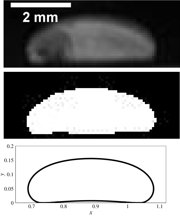
From experiments, the typical time scale of the phenomenon is noted to be of the order of fraction of a second, and thus it is recorded at a high frame frequency of 2000 frames per second for a sufficient temporal resolution using a monochromatic camera (Phantom v7.0). Due to small size of the cell, the original gray scale image of the droplet is not very clear, as can be noticed in figure 2. For this, we zoom near the relevant portion of the domain and then sharpen the images, converting them to binary form. Eventually the phase boundaries are then extracted from the binary image data, shown in figure 23. This sequence gives a comparatively clear description of the interface of the droplet. The image-processing sufficiently resolves the changes in the configuration of the interface and the dynamics of the tail of the droplet during its rise. After calibrating the frames for further measurements, an co-ordinate system is chosen with its origin placed at the center of the bottom wall (figure 23). The co-ordinates are measured in . The time instant at which the droplet just starts experiencing the influence of the magnetic field is marked as .

The domain dimensions, the droplet size at the initial condition and the details about the pixel resolutions of the area covering the droplet and the domain, are given in table 3, while the fluid properties were given in table 1. In this simulation set, we use the fluid properties and other relevant parameters in their dimensional form, so that the results can directly be compared with the experimental measurements. Standard properties of water are taken for . For properties of , the FF sample has been characterized, except for its interfacial tension with water. For this we use the method of Zhu et al. (2011a) where the researchers compared the initial conditions of the experiment and simulation to determine the coefficient of interfacial tension. Using this approach we predict that . The initial shape of the droplet in simulations compares well with the experimental initial shape. The comparison is shown in figure 22 (right). The magnetization curve for the ferrofluid sample has been characterized using a EverCool SQUID VSM DC magnetometer and it is shown in figure 22. The initial susceptibility and saturation magnetization , as depicted from the magnetization curve, are and respectively. Thus the FF sample is weakly magnetizable and a shorter levitation height of the water droplet is expected.
9.1 Singularity at the tail of the droplet
The shapes of the droplet at different instants of time from the experiment and simulation are compared in figure 24. For above characterized samples of fluids, we notice that the levitation height is small, which is due to the weakly magnetizable nature of the ferrofluid sample (). Interestingly, a formation of singular projection at the tail of the levitating droplet is observed in both the experiment and the simulation. The central portion of the tail of the droplet remains adhered in the vicinity of the bottom wall for some initial time, although there is a layer of ferrofluid separating it from the bottom wall. The width of this adhered part of the interface reduces gradually and approximately at in the experiment, it detaches completely. The singularity is formed after this instant at the tail of the droplet (). As the droplet levitates, the singular point appears to being pulled towards the bulk of the droplet. Eventually the singularity disappears and the droplet tail becomes smooth and concave downward. The simulations have predicted this phenomenon reasonably well. It also strongly support our argument in §6 that the interfacial singularities or cusps at the interface of the levitating droplet in a ferrofluid can be ubiquitous, especially for low interfacial tension (low ).
As initially a segment of the droplet interface is settled near the bottom wall, the field strength along this portion of the interface is approximated as , according to the field boundary condition at the bottom wall. For a small initial time we assume that the magnetic field at this segment of the interface is close to the field value at the wall itself. The order of the vertical magnetic force on this segment of the interface is then , where is the permeability difference across the interface. Using the field strength along this interface segment, . For small initial period of time the segment will rise faster if at the wall is higher and vice-versa. If the displaced vertical location of this segment after is , then . The squared sine interface description at the tail of the droplet is closely resembled at in simulations and at in experiments in figure 24, where the tip of the projection is still close to the wall and is not cusped (also indicated by smoothness of ). However, at relatively larger time the feature transits towards a cusp, and the approximation that the field value at the segment equal to the field value at the bottom wall is no more valid. After this regime, the hydrodynamic and the effect of higher outer liquid viscosity (see §6) becomes significant.
The sharp singular tips are observed in droplet systems, for example in Stone et al. (1999) under electric field and by Rowghanian et al. (2016) for magnetic drop under uniform magnetic field. Stone et al. (1999) have concluded that the conical tips appear for certain threshold electric field strength and the dielectric constant ratio. Rowghanian et al. (2016) focused curved tip regimes, however, they clearly discuss that the sharp tips are possible due to destabilization of the droplet under high field strengths and high localization of the magnetic stresses at the droplet poles. In present study the situation is, however, dynamic and the field is non-uniform. A low interfacial tension (low Laplace number ) in combination with the hydrodynamic viscous stress difference (exhibited through viscosity ratio change) across the interface are two additional important factors which can help realizing such sharp conical tips. In practical situations, the former is reasonably modifiable using a surfactant solution and the latter by taking a different non-magnetic droplet medium in a ferrofluid (or a non-magnetic medium outside a ferrofluid droplet).
Although the droplet is essentially moving in a quasi-two dimensional cell, and it might be more appropriate to use gap-averaged Navier-Stokes equations, it turns out that the current 2D mathematical description captures the droplet’s shape reasonably well. Thus the spatial solution is quite accurate. However during the later stages of the droplet rise, the solution is temporally deviating (Fig. 24). As far as the spatial shapes of the droplet are concerned, any 3D effects due to the out-of-plane curvature of the droplet in the Hele-Shaw gap are not dominant. We attribute the accurate capturing of the droplet interface shape to the following points — (a) careful characterization of the ferrofluid sample’s non-linear magnetization curve, as well as some other properties, and implementing the same in the simulations using the Langevin’s non-linear magnetization model (Fig. 22), (b) implementing the initial interface condition precisely similar to one which we find for a resting droplet in the experiments, (c) convenience in closely realizing the actual field boundary-conditions due to the Halbach-array, (d) modeling similar flow boundary-conditions as that in experiments, and (e) using some state-of-the-art numerical techniques for computational accuracy. In addition, the ferrofluid sample in the experiments is characterized and found to be weakly magnetizable. The numerical solution is then expected to be more accurate due to less sharper change of the magnetic properties and field (and thus a softer jump in the magnetic force term in the NS equations) across the interface. The possible reasons why temporally the 2D assumption is only reasonable might be due to the following unrelaxed assumptions — (a) neglecting the out-of-plane curvature in simulations due to H-S geometry, or in other words, neglecting the quasi-2D nature of the problem and considering it as a 2D problem in simulations, (b) neglecting one very important aspect of the magnetization-relaxation dynamics in ferrofluids and considering instantly relaxing magnetization when the magnetic field changes. We believe that incorporation of the magnetization relaxation time effect coupled with a two-phase model for ferrofluid interface, together with corrections due to the third dimension (e.g. implementing the Darcy law (Gondret & Rabaud, 1997) together with inertial corrections to it (Ruyer-Quil, 2001)), can closely resolve the temporal details also.
10 Dynamical model
A differential model for the vertical trajectory of the levitating droplet is constructed to obtain an analytical expressions for the onset condition of levitation, levitation height, and conditions for transitions in the droplet time response near the equilibrium. This was previously analyzed by the displacement and velocity plots from the simulations in §5.4. In this model, the levitation path is assumed to be stable in the lateral direction and thus the droplet is assumed to move only in the vertical dimension. A single magnetic source of strength is considered at the bottom wall while no source is assumed on the side or top. Additionally, we assume the droplet to be spherical. For simplicity of the formulation, the local magnetic field distortions due to the presence of the droplet are neglected, and the local filed is assumed equal to a local field which would be present if there is no droplet. At any time , if the vertical position of the droplet is denoted by , then the Newton’s equation of motion for the droplet can be written as
| (35) |
where is the field strength along the vertical direction . We assume that the field strength decays as from the magnetic source of strength at with a decay constant (in units of ). Notice that is negative and thus provides a positive upward levitation force. The above equation describing the decay of the magnetic field along the vertical direction ( or ) is assumed to be valid only along the vertical direction but only away from the bottom wall, due to the fact that the droplet’s initial location in simulations was considered above the bottom wall (see for example figure 4). Using this in equation 35, and rearranging, we get
| (36) |
To compare the vertical trajectories with simulations, the above equation is non-dimensionalized using the same reference scales used in equation 11, which casts it in terms of and as
| (37) |
where , and the right hand side is basically a non-linear forcing function due to the magnetic source. For simplicity, we write the above equation as
| (38) |
The equation is sensitive to four parameters – , and the non-dimensional constant carrying information about the vertically decaying magnetic field strength.
10.1 Levitation height and onset condition
The differential equation 38 is a second order ordinary but non-linear due to the form of . It is reduced to a first order system of two differential equations by introducing a variable , written as
| (39) |
The long-time equilibrium or fixed point of the system is obtained by setting the droplet speed , and acceleration to in 39, which for non-zero , gives the steady state fixed point
| (40) |
As , it turns out that
| (41) |
The steady state levitation height of the droplet depends on parameter and the ratio (which is ), and is independent of the parameter . This is expected as is the strength of the viscous drag force opposing the droplet motion and it must vanish at steady state. If the levitation height is to be a non-zero positive, then , which provides the condition for the onset of levitation
| (42) |
where is constant. If the onset condition is satisfied, the levitation height is
| (43) |
The above expression is physically is in agreement with the facts – the rise of the droplet will increase in a ferrofluid sample of higher permeability, with lower droplet mass densities, with the increase in or decrease in .
10.2 Transition in the nature of the fixed point
The transitions in the nature of the fixed point are reveled by evaluating the eigenvalues of the Jacobian for the system 39, which is
| (44) |
If are the eigenvalues of , then the characteristic equation is and the eigenvalues or the characteristic values of the fixed point, , are . This gives the possibilities (distinct real eigenvalues), (identical real eigenvalues), and (complex conjugate eigenvalues).

The first case physically suggests that the fixed point is of type node and the droplet will approach the steady state monotonically. The third case of complex eigenvalues, however, suggest that the fixed point is of type spiral and the droplet will oscillate around the fixed point before reaching the steady state. The second case gives the critical value of the parameter , at which the stable fixed point changes its type from spiral to node or vice-versa, according to
| (45) |
Thus from the condition of complex conjugate eigenvalues, , the oscillations around the equilibrium point do occur if
| (46) |
where is constant. It is important to note that the parameter do not influence the condition for the oscillations around the equilibrium, it only appears in the expression of the steady state levitation height.
The nature of the stable fixed point and transitions in its behavior is further studied through phase portraits on plane. The differential equation for from 39 is
| (47) |
Using this, first we show the effect of variation of ( viscosity ratio) at fixed () and (). This is depicted in figure 25 for different initial conditions on a circle around the fixed point. For , , and thus we vary around . The behavior of the linearized solution around the fixed point is clearly sensitive to , although the actual magnitude of depends on . The variation in changes the nature of the fixed point from being a spiral to a monotonic attractor at . This observation is in well agreement with the simulations in figure 9 and 10, where the transition between monotonicity and oscillations of the curves were noted.
We conclude by explicitly comparing the solution of the analytical model 37 to the simulations of figure 9. In simulations we noted that the response changes from monotonic to undulatory when is increased (figure 9). Here we take the extreme cases of and considered there. The comparison is shown in figure 26. The corresponding trajectories on () plane are also depicted in the inset. The value is chosen from the results of figure 9 such that the ratio is more or less the same in the dynamical model. This results in nearly same final levitation height according to , and thus only the nature of response can be closely compared. We have obtained a reasonable agreement between the simulations and the dynamical model about the statement of transition between monotonic to undulatory droplet levitation.
Thus the model captures the essential features of the levitation dynamics of the droplet, and at the same time, it provides a simpler alternative in place of full fledged simulations to predict the condition for the onset of levitation, the levitation height, the condition for oscillations around the equilibrium and the nature of the solution around the equilibrium. The model, however, do not care about the lateral stability of the levitation path. Those conditions for the lateral stability needed a coupled analysis of the magnetic field and the flow solutions (§8).
11 Conclusions and discussion
In this study, we show that the stable levitation of a non-magnetizable droplet immersed inside a ferrofluid is possible with the help of an appropriately generated spatially non-uniform magnetic field; the levitation can be unstable, or can have multiple-stable states, essentially depending upon the spatially inhomogeneous magnetic field strength. The dynamics of the levitating droplet is analyzed primarily through computations based on a conservative finite-volume based pressure projection algorithm coupled with a multigrid solver for the magnetic field solution and the front-tracking algorithm for the interfacial advections. Physical demonstrations to support the simulations are presented. A dynamical model is proposed for the prediction of the onset of levitation, the steady state levitation height, and the time evolution of the droplet in the vertical direction. In this inverse system, where the droplet is non-magnetizable and the outer liquid is ferrofluid, the droplet is forced in the direction opposite to the field gradient.
The conclusions from the study are focused in terms of the following three fundamental curiosities - (a) the shape of the levitating droplet and the appearance of interfacial singularity, (b) the stability of the levitation path and the existence of multiple possible final states, and (c) the nature of the droplet time response around the steady state levitation point. The conclusions about these three aspects from our study are discussed below one by one.
a. The shape of the levitating droplet and the appearance of interfacial singularity.
The non-magnetizable droplet levitation in a ferrofluid is simulated inside a bounded square domain under the magnetic field generated by a Halbach array of magnets. The system in general is sensitive to the Laplace number , the magnetic Laplace number and the Galilei number . The shape of the levitating droplet primarily depends on the magnitudes of and ; the dependence being apparent only at low . The shape is weakly influenced by the changes in . For high , the shape of the droplet remains nearly circular, or at most, attains only a slight deformation. On the other hand, the deformation can be more pronounced at low due to spatially complex magnetic field. Also, this minor deviation from the circular shape in case of higher occurs only during the initial transience. As the number decreases, the deformation of the interface at the tail of the droplet increases. The deformation becomes more pronounced for of order . In this regime, unique shapes of the levitating droplet are observed, e.g, the segmented-ring, crescent and tooth-like; the shape transitions from one type to another occur over time or with change of the above control parameters.
The above observations are for the droplet having viscosity higher than that of the ferrofluid. If the viscosity of the droplet is lower than that of the ferrofluid, it is noticed that the local dynamics of the interface alters. Under these circumstances, the tail of the droplet might show cusped features at sufficiently high . The previously discussed crescent-like shapes now approach exact crescent shapes. It is shown that there is a possibility of the appearance of singularities at the surface of the non-magnetizable droplet during its field guided motion inside ferrofluid; such singular projection at the tail of the droplet is physically demonstrated and also predicted by the simulation.
The deformation of the droplet is also sensitive to the degree of non-linearity in the magnetization curve of the ferrofluid sample. A change of even one order in the magnitude of the parameter can significantly alter the droplet shape, nature of interfacial projections and the levitation height.
b. The stability of the levitation path.
The path of the levitating droplet has shown quite a sensitivity to the spatial description of the magnetic field; not every arrangement of magnets can provide a stable levitation mechanism. The motion of the non-magnetic droplet, and the flow resulting due to this motion, is primarily due to the application of the magnetic field gradient and is parallel to . But interestingly if the horizontal symmetry of the field around the initial location of the droplet is not maintained, the flow vortices generated near the tail projections of the droplet can be capable of deviating the droplet from its path parallel to . The magnetic forces and the resulting flow show mutually competing influences on the trajectory of the levitating droplet and this interaction can cause the droplet trajectory to go away from what is expected. We show that appropriate magnetic arrangement can constrain this instability of the droplet levitation path.
c. The nature of the droplet time response and the existence of multiple possible final states.
Besides the levitation path, the stability of the final equilibrium location of the droplet is also investigated. It is found that there may exist magnetic fields which can give rise to multiple stable states of the levitated droplet. The regions of minima of the magnetic field strength, local or global, act as attractors to the droplet. If the magnet arrangement generates multiple such local minima, multiple stable states can exist. The final equilibrium of the droplet is then affected by the initial location of the droplet and its relative distance to various regions of field minima.
The onset condition for the levitation, the temporal evolution of the droplet, its steady state levitation height and the nature of the stationary point are predicted by a dynamical model, provided that the droplet levitation path is laterally stable/constrained. The model has verified the statement, which was initially based on the simulations, that the response of the droplet can be either monotonic, or it can oscillate about the equilibrium location before reaching to the steady state depending upon the viscosity ratio, density ratio and . Specifically a transition between a stable spiral and a stable node is identified; the transition between the two occur at , and the steady state levitation height can be quickly predicted by .
12 Acknowledgements
Authors gratefully thank fruitful discussions with Prof. Sandipan Ghosh Moulic. Authors also thank the Council for Scientific and Industrial Research, New-Delhi, for partial funding. A preliminary part of the work was presented at the International Conference on Multiphase Flow, 2016, Florence, Italy.
Appendix A Grid and time step independence
To study the grid and time step independency of the simulations, a combination of non-dimensional groups is first selected, from the range simulated in the present study, for which the droplet goes under maximum deformation and levitation height. It is intuited that a grid resolution which is sufficient for this extreme case will serve the purpose for the rest of the simulation sets. For constant permeability assumption, the droplet deformation is maximum for and its levitation is maximum when and . For variable permeability the same is true for and .
|
|||||||
|---|---|---|---|---|---|---|---|
|
Thus for these set of parameters, we resolve the grid starting from to and look for the saturation in the outcomes at some grid resolution. Here is the diameter of the round droplet and is the computational cell size. The outcomes judged are the interface shapes (figure 27 under constant permeability assumption and figure 28 for variable permeability case) and the relative mean percentage error in the droplet deformation parameter curve (table 4 and figure 29). The grid resolution of has proven to be a reasonable choice.
Likewise, the time independence of the simulations is also assured by comparing the signature of the droplet deformation parameter with respect to time for different time steps (figure 30). The simulations have shown time step independence at . The droplet shapes are also found to be independent of the time step below , and thus this value is adopted.
References
- Afkhami et al. (2008) Afkhami, S, Renardy, Y, Renardy, M, Riffle, JS & St Pierre, T 2008 Field-induced motion of ferrofluid droplets through immiscible viscous media. Journal of Fluid Mechanics 610, 363–380.
- Afkhami et al. (2010) Afkhami, S, Tyler, AJ, Renardy, Y, Renardy, M, St Pierre, TG, Woodward, RC & Riffle, JS 2010 Deformation of a hydrophobic ferrofluid droplet suspended in a viscous medium under uniform magnetic fields. Journal of Fluid Mechanics 663, 358–384.
- Bacri et al. (1994) Bacri, J-C, Cebers, AO & Perzynski, R 1994 Behavior of a magnetic fluid microdrop in a rotating magnetic field. Physical review letters 72 (17), 2705.
- Bacri & Salin (1983) Bacri, J-C & Salin, D 1983 Bistability of ferrofluid magnetic drops under magnetic field. Journal of Magnetism and Magnetic Materials 39 (1), 48–50.
- Bashtovoi et al. (1999) Bashtovoi, V, Pogirnitskaya, S & Reks, A 1999 Dynamics of deformation of magnetic fluid flat drops in a homogeneous longitudinal magnetic field. Journal of magnetism and magnetic materials 201 (1), 300–302.
- Beysens & van Loon (2015) Beysens, Daniel A & van Loon, Jack JWA 2015 Generation and applications of extra-terrestrial environments on earth. River Publishers.
- Chen & Cheng (2008) Chen, Ching-Yao & Cheng, Z-Y 2008 An experimental study on rosensweig instability of a ferrofluid droplet. Physics of Fluids (1994-present) 20 (5), 054105.
- Chen & Li (2010) Chen, Ching-Yao & Li, C-S 2010 Ordered microdroplet formations of thin ferrofluid layer breakups. Physics of Fluids (1994-present) 22 (1), 014105.
- Dunne et al. (2007) Dunne, PA, Hilton, J & Coey, JMD 2007 Levitation in paramagnetic liquids. Journal of magnetism and magnetic materials 316 (2), 273–276.
- Duplat & Mailfert (2013) Duplat, Jérôme & Mailfert, Alain 2013 On the bubble shape in a magnetically compensated gravity environment. Journal of Fluid Mechanics 716, R11.
- Fattah et al. (2016) Fattah, Abdel Rahman Abdel, Ghosh, Suvojit & Puri, Ishwar K 2016 Printing microstructures in a polymer matrix using a ferrofluid droplet. Journal of Magnetism and Magnetic Materials 401, 1054–1059.
- Geim et al. (1999) Geim, AK, Simon, MD, Boamfa, MI & Heflinger, LO 1999 Magnet levitation at your fingertips. Nature 400 (6742), 323.
- Gondret & Rabaud (1997) Gondret, P & Rabaud, M 1997 Shear instability of two-fluid parallel flow in a hele–shaw cell. Physics of Fluids 9 (11), 3267–3274.
- Gu et al. (2015) Gu, Yu, Bragheri, Francesca, Valentino, Gianna, Morris, Karl, Bellini, Nicola & Osellame, Roberto 2015 Ferrofluid-based optofluidic switch using femtosecond laser-micromachined waveguides. Applied optics 54 (6), 1420–1425.
- Gu et al. (2016) Gu, Yu, Chow, Huiyanangel & Morris, Karl 2016 Motion of ferrofluid droplets under oscillating magnetic field. Bulletin of the American Physical Society .
- Halbach (1985) Halbach, Klaus 1985 Application of permanent magnets in accelerators and electron storage rings. Journal of Applied Physics 57 (8), 3605–3608.
- Huber & Littke (1996) Huber, Felix & Littke, Walter 1996 Technology experiments for magnetic levitation in transparent ferrofluids. In Space Station Utilisation, , vol. 385, p. 479.
- Ikezoe et al. (1998) Ikezoe, Yasuhiro, Hirota, Noriyuki, Nakagawa, Jun & Kitazawa, Koichi 1998 Making water levitate. Nature 393 (6687), 749–750.
- Jackson & Miranda (2007) Jackson, DP & Miranda, JA 2007 Confined ferrofluid droplet in crossed magnetic fields. The European Physical Journal E 23 (4), 389–396.
- Jackson (2005) Jackson, David P 2005 Theory, experiment, and simulations of a symmetric arrangement of quasi-two-dimensional magnetic fluid drops. Journal of magnetism and magnetic materials 289, 188–191.
- Kim et al. (2015) Kim, D, Yu, S, Kang, B-G & Yun, K-S 2015 Liquid-based electrostatic energy harvester using rotational motion of ferrofluid droplets. In Solid-State Sensors, Actuators and Microsystems (TRANSDUCERS), 2015 Transducers-2015 18th International Conference on, pp. 59–61. IEEE.
- Kim & Yun (2015) Kim, D & Yun, KS 2015 Energy harvester using contact-electrification of magnetic fluid droplets under oscillating magnetic field. In Journal of Physics: Conference Series, , vol. 660, p. 012108. IOP Publishing.
- Kim & Lim (2015) Kim, Hun & Lim, HeeChang 2015 Mode pattern of internal flow in a water droplet on a vibrating hydrophobic surface. The Journal of Physical Chemistry B .
- Koh et al. (2013) Koh, Wei Hang, Lok, Khoi Seng & Nguyen, Nam-Trung 2013 A digital micro magnetofluidic platform for lab-on-a-chip applications. Journal of Fluids Engineering 135 (2), 021302.
- Korlie et al. (2008) Korlie, Mark S, Mukherjee, Arup, Nita, Bogdan G, Stevens, John G, Trubatch, A David & Yecko, Philip 2008 Modeling bubbles and droplets in magnetic fluids. Journal of Physics: Condensed Matter 20 (20), 204143.
- Kovalchuk & Vollhardt (2001) Kovalchuk, NM & Vollhardt, D 2001 A numerical study of surface tension auto-oscillations. effect of surfactant properties. The Journal of Physical Chemistry B 105 (20), 4709–4714.
- Limbach et al. (2016) Limbach, Christopher M, Robinson, Ryan, Adams, Dylan, Wilbanks, Megan & Yalin, Azer P 2016 Toward a microscopic study of laser interactions with levitated liquid fuel droplets .
- Lira & Miranda (2016) Lira, Sérgio A & Miranda, José A 2016 Ferrofluid patterns in hele-shaw cells: Exact, stable, stationary shape solutions. Physical Review E 93 (1), 013129.
- Liu et al. (2011a) Liu, Jing, Tan, Say-Hwa, Yap, Yit Fatt, Ng, Min Yuan & Nguyen, Nam-Trung 2011a Numerical and experimental investigations of the formation process of ferrofluid droplets. Microfluidics and nanofluidics 11 (2), 177–187.
- Liu et al. (2011b) Liu, Jing, Yap, Yit Fatt & Nguyen, Nam-Trung 2011b Numerical study of the formation process of ferrofluid droplets. Physics of Fluids (1994-present) 23 (7), 072008.
- Liu et al. (2014) Liu, S, Yi, Xiang, Leaper, Mark & Miles, NJ 2014 Horizontal deflection of single particle in a paramagnetic fluid. The European Physical Journal E 37 (6), 1–9.
- Mirica et al. (2009) Mirica, Katherine A, Shevkoplyas, Sergey S, Phillips, Scott T, Gupta, Malancha & Whitesides, George M 2009 Measuring densities of solids and liquids using magnetic levitation: Fundamentals. Journal of the American Chemical Society 131 (29), 10049–10058.
- Mugele et al. (2006) Mugele, F, Baret, JC & Steinhauser, D 2006 Microfluidic mixing through electrowetting-induced droplet oscillations. Applied Physics Letters 88 (20), 204106–204106.
- Nguyen (2013) Nguyen, Nam-Trung 2013 Deformation of ferrofluid marbles in the presence of a permanent magnet. Langmuir 29 (45), 13982–13989.
- Olaru et al. (2013) Olaru, R, Petrescu, Camelia & Arcire, A 2013 Maximizing the magnetic force generated by an actuator with non-magnetic body in a ferrofluid pre-magnetized by permanent magnets. International Review of Electrical Engineering (IREE) 8 (2), 904–911.
- Pamme (2006) Pamme, Nicole 2006 Magnetism and microfluidics. Lab on a Chip 6 (1), 24–38.
- Price et al. (2015) Price, CJ, Giltrap, S, Stuart, NH, Parker, S, Patankar, S, Lowe, HF, Smith, RA, Donnelly, TD, Drew, D, Gumbrell, ET & others 2015 An in-vacuo optical levitation trap for high-intensity laser interaction experiments with isolated microtargets. Review of Scientific Instruments 86 (3).
- Rosenkilde (1969) Rosenkilde, CE 1969 A dielectric fluid drop an electric field. In Proceedings of the Royal Society of London A: Mathematical, Physical and Engineering Sciences, , vol. 312, pp. 473–494. The Royal Society.
- Rosensweig (1966) Rosensweig, RE 1966 Buoyancy and stable levitation of a magnetic body immersed in a magnetizable fluid. Nature 210, 613–614.
- Rosensweig (1985) Rosensweig, Ronald E 1985 Ferrohydrodynamics. Cambridge University Press.
- Rowghanian et al. (2016) Rowghanian, P, Meinhart, CD & Campàs, O 2016 Dynamics of ferrofluid drop deformations under spatially uniform magnetic fields. Journal of Fluid Mechanics 802, 245–262.
- Ruyer-Quil (2001) Ruyer-Quil, Christian 2001 Inertial corrections to the darcy law in a hele–shaw cell. Comptes Rendus de l’Académie des Sciences-Series IIB-Mechanics 329 (5), 337–342.
- Sandre et al. (1999) Sandre, O, Browaeys, J, Perzynski, R, Bacri, J-C, Cabuil, V & Rosensweig, RE 1999 Assembly of microscopic highly magnetic droplets: Magnetic alignment versus viscous drag. Physical Review E 59 (2), 1736.
- Sero-Guillaume et al. (1992) Sero-Guillaume, OE, Zouaoui, D, Bernardin, D & Brancher, JP 1992 The shape of a magnetic liquid drop. Journal of Fluid Mechanics 241, 215–232.
- Sherwood (1988) Sherwood, JD 1988 Breakup of fluid droplets in electric and magnetic fields. Journal of Fluid Mechanics 188, 133–146.
- Singh et al. (2016a) Singh, Chamkor, Das, Arup Kumar & Das, Prasanta Kumar 2016a Flow restrictive and shear reducing effect of magnetization relaxation in ferrofluid cavity flow. Physics of Fluids (1994-present) 28 (8), 087103.
- Singh et al. (2016b) Singh, Chamkor, Das, Arup K & Das, Prasanta K 2016b Single-mode instability of a ferrofluid-mercury interface under a nonuniform magnetic field. Physical Review E 94 (1), 012803.
- Stone et al. (1999) Stone, Howard A, Lister, John R & Brenner, Michael P 1999 Drops with conical ends in electric and magnetic fields. In Proceedings of the Royal Society of London A: Mathematical, Physical and Engineering Sciences, , vol. 455, pp. 329–347. The Royal Society.
- Tan et al. (2010) Tan, Say-Hwa, Nguyen, Nam-Trung, Yobas, Levent & Kang, Tae Goo 2010 Formation and manipulation of ferrofluid droplets at a microfluidic t-junction. Journal of Micromechanics and Microengineering 20 (4), 045004.
- Taylor (1964) Taylor, Geoffrey 1964 Disintegration of water drops in an electric field. In Proceedings of the Royal Society of London A: Mathematical, Physical and Engineering Sciences, , vol. 280, pp. 383–397. The Royal Society.
- Timonen et al. (2013) Timonen, Jaakko VI, Latikka, Mika, Leibler, Ludwik, Ras, Robin HA & Ikkala, Olli 2013 Switchable static and dynamic self-assembly of magnetic droplets on superhydrophobic surfaces. Science 341 (6143), 253–257.
- Trinh (1985) Trinh, EH 1985 Compact acoustic levitation device for studies in fluid dynamics and material science in the laboratory and microgravity. Review of Scientific Instruments 56 (11), 2059–2065.
- Tryggvason et al. (2011) Tryggvason, Grétar, Scardovelli, Ruben & Zaleski, Stéphane 2011 Direct numerical simulations of gas–liquid multiphase flows. Cambridge University Press.
- Ueno et al. (1995) Ueno, Kazuyuki, Higashitani, Masaru & Kamiyama, Shinichi 1995 Study on single bubbles rising in magnetic fluid for small weber number. Journal of magnetism and magnetic materials 149 (1-2), 104–107.
- Ueno et al. (1999) Ueno, Kazuyuki, Nishita, Takeshi & Kamiyama, Shinichi 1999 Numerical simulation of deformed single bubbles rising in magnetic fluid. Journal of magnetism and magnetic materials 201 (1), 281–284.
- Unverdi & Tryggvason (1992) Unverdi, Salih Ozen & Tryggvason, Grétar 1992 A front-tracking method for viscous, incompressible, multi-fluid flows. Journal of computational physics 100 (1), 25–37.
- Verkouteren & Verkouteren (2011) Verkouteren, R Michael & Verkouteren, Jennifer R 2011 Inkjet metrology ii: resolved effects of ejection frequency, fluidic pressure, and droplet number on reproducible drop-on-demand dispensing. Langmuir 27 (15), 9644–9653.
- Vojtíšek et al. (2012) Vojtíšek, Martin, Tarn, Mark D, Hirota, Noriyuki & Pamme, Nicole 2012 Microfluidic devices in superconducting magnets: on-chip free-flow diamagnetophoresis of polymer particles and bubbles. Microfluidics and nanofluidics 13 (4), 625–635.
- Whitehill et al. (2011) Whitehill, James, Neild, Adrian, Ng, Tuck Wah, Martyn, Steven & Chong, Jonathan 2011 Droplet spreading using low frequency vibration. Applied Physics Letters 98 (13), 133503.
- Wohlhuter & Basaran (1993) Wohlhuter, Fred K & Basaran, Osman A 1993 Effects of physical properties and geometry on shapes and stability of polarizable drops in external fields. Journal of magnetism and magnetic materials 122 (1-3), 259–263.
- Wojciechowski & Kucharek (2009) Wojciechowski, Kamil & Kucharek, Marta 2009 Interfacial tension oscillations without surfactant transfer. The Journal of Physical Chemistry B 113 (41), 13457–13461.
- Wu et al. (2013) Wu, Yining, Fu, Taotao, Ma, Youguang & Li, Huai Z 2013 Ferrofluid droplet formation and breakup dynamics in a microfluidic flow-focusing device. Soft Matter 9 (41), 9792–9798.
- Zhu et al. (2011a) Zhu, Gui-Ping, Nguyen, Nam-Trung, Ramanujan, Raju V & Huang, Xiao-Yang 2011a Nonlinear deformation of a ferrofluid droplet in a uniform magnetic field. Langmuir 27 (24), 14834–14841.
- Zhu (2013) Zhu, Taotao 2013 Microfluidic continuous-flow manipulation of particles and cells inside ferrofluids. uga.
- Zhu et al. (2011b) Zhu, Taotao, Lichlyter, Darcy J, Haidekker, Mark A & Mao, Leidong 2011b Analytical model of microfluidic transport of non-magnetic particles in ferrofluids under the influence of a permanent magnet. Microfluidics and Nanofluidics 10 (6), 1233–1245.