跳到论文正文
W Papers独立论文阅读器 arXiv:1712.01172 论文正文 计算阅读时间 · 0%
引用这篇论文根据当前论文元数据生成,正式投稿前建议核对。


License: arXiv.org perpetual non-exclusive license
arXiv:1712.01172v3 [math.AP] 27 Sep 2019

Fractal homogenization of multiscale interface problems

Martin Heida, Ralf Kornhuber, and Joscha Podlesny
Abstract.

Inspired by continuum mechanical contact problems with geological fault networks, we consider elliptic second order differential equations with jump conditions on a sequence of multiscale networks of interfaces with a finite number of non-separating scales. Our aim is to derive and analyze a description of the asymptotic limit of infinitely many scales in order to quantify the effect of resolving the network only up to some finite number of interfaces and to consider all further effects as homogeneous. As classical homogenization techniques are not suited for this kind of geometrical setting, we suggest a new concept, called fractal homogenization, to derive and analyze an asymptotic limit problem from a corresponding sequence of finite-scale interface problems. We provide an intuitive characterization of the corresponding fractal solution space in terms of generalized jumps and gradients together with continuous embeddings into L2L^{2} and HsH^{s}, s<1/2s<1/2. We show existence and uniqueness of the solution of the asymptotic limit problem and exponential convergence of the approximating finite-scale solutions. Computational experiments involving a related numerical homogenization technique illustrate our theoretical findings.

This research has been funded by Deutsche Forschungsgemeinschaft (DFG) through grant CRC 1114 ”Scaling Cascades in Complex Systems”, Project C05 ”Effective models for interfaces with many scales” and Project B01 ”Fault networks and scaling properties of deformation accumulation”.

1. Introduction

Classical elliptic homogenization is concerned with second order differential equations of the form

(1) −∇(Aε∇uε)=f,-\nabla\left(A^{\varepsilon}\nabla u_{\varepsilon}\right)=f\,,

denoting Aε​(x)=A​(xε)A^{\varepsilon}(x)=A\left(\frac{x}{\varepsilon}\right) with ε>0\varepsilon>0 and some uniformly bounded, positive coefficient field AA. Hence, AεA^{\varepsilon} is oscillating on a spatial scale of size ε\varepsilon compared to the diameter of the macroscopic computational domain 𝑸⊂ℝd\boldsymbol{Q}\subset\mathbb{R}^{d}. In periodic homogenization, the coefficient AA is Y\mathrm{Y}-periodic, where Y=[0,1[d\mathrm{Y}=[0,1[^{d} is the unit cell in ℝd\mathbb{R}^{d}. In stochastic homogenization, the coefficient Aε​(x)=Aω​(xε)A^{\varepsilon}(x)=A_{\omega}\left(\frac{x}{\varepsilon}\right) is a stationary (i.e. statistically shift invariant) and ergodic (asymptotically uncorrelated) random variable on a probability space (Ω,ℱ,P)(\Omega,\mathcal{F},P) with ω∈Ω\omega\in\Omega. A variety of results have been derived in the field of homogenization, and we refer to [1, 2, 11, 22] for the periodic case and to [24, 37] for the stochastic case. For error estimates in homogenization, we refer to [3, 4, 11, 17, 18]. Mathematical modelling of polycrystals or composite materials typically leads to elliptic interface problems with appropriate jump conditions on a microscopic interface Γε⊂𝑸\Gamma^{\varepsilon}\subset\boldsymbol{Q}. A periodic setting is obtained by Γε=ε​Γ0\Gamma^{\varepsilon}=\varepsilon\Gamma_{0} with scaling parameter ε>0\varepsilon>0 and a piecewise smooth hypermanifold Γ0\Gamma_{0} with Y\mathrm{Y}-periodic cells. The size of the cells is then of order ε\varepsilon compared to the macroscopic domain. Denoting by \lsem​uε​\rsemν\lsem u_{\varepsilon}\rsem_{\nu} the jump of uεu_{\varepsilon} in normal direction ν\nu on Γε\Gamma^{\varepsilon}, the condition

(2) −∂νuε=\lsemuε\rsemν-\partial_{\nu}u_{\varepsilon}=\lsem u_{\varepsilon}\rsem_{\nu}

on the normal derivatives ∂νuε\partial_{\nu}u_{\varepsilon} is imposed at the boundary of each cell. Corresponding stochastic variants have been studied in [20, 23]. The homogenization of such kind of periodic multiscale interface problems has been studied in great detail, see [12, 13, 19, 21] and references therein. Similar concepts have been applied to foam-like elastic media like the human lung, cf., e.g., [5, 10]. Classical (stochastic) homogenization relies on periodicity (or ergodicity) and scale separation. The latter means that homogenized problems in the asymptotic limit ε→0\varepsilon\to 0 usually decouple into a global problem that describes the macroscopically observed behavior of the system, and one or more local problems, often referred to as cell-problems, that capture the oscillatory behavior.

In contrast to analytic homogenization, numerical homogenization addresses the lack of regularity of solutions of problems with highly oscillatory coefficients AεA^{\varepsilon} in numerical computations, either by local corrections of standard finite elements [14, 28] or by multigrid-type iterative schemes [26, 27]. Both approaches are closely related [25] and usually do not rely on periodicity or scale separation.

In this work, we consider elliptic multiscale interface problems without scale separation in a non-periodic geometric setting motivated by geology. Experimental studies suggest that grains in fractured rock are distributed in a fractal manner [30, 34]. In particular, this means that the size of grains and interfaces follows an exponential law: The total number N⁡(r)N(r) of grains larger than some r>0r>0 behaves according to

(3) N⁡(r)=C​r−DN(r)=Cr^{-D}\,

and DD is often called the fractal dimension. This observation is also captured by geophysical modelling of fragmentation by tectonic deformation [33] which is based on the assumption that deformation of two neighboring blocks of equal size might lead to fracturing in one of these blocks. It is unlikely and therefore excluded in this model, that bigger blocks break smaller ones or vice versa. A typical example for corresponding multiscale interface networks is given by the Cantor-type geometry [34] as depicted in Figure 1. While each level-KK interface network Γ(K)\Gamma^{(K)} clearly is two-dimensional, the limiting multiscale network Γ=Γ(∞)\Gamma=\Gamma^{(\infty)} has fractal dimension ln⁡6/ln⁡2\ln 6/\ln 2, which is in good agreement with experimental studies that often yield D≈2.5D\approx 2.5. Observe that the cells representing the different grains are not periodically distributed. They can also be arbitrarily small and cover the whole range up to half of the given domain 𝑸\boldsymbol{Q} so that there is no scale parameter ε\varepsilon separating a small from a large scale. Similar geometric settings, but with a completely different scope, occur for thin fractal fibers [29].

Figure 1. Level-KK interface network Γ(K)\Gamma^{(K)} for K=4K=4, 55, and 66, taken from [34].

Geological applications give rise to continuum mechanical problems with frictional contact on such multiscale networks of interfaces or faults. The level-KK network Γ(K)=⋃k=1KΓk\Gamma^{(K)}=\bigcup_{k=1}^{K}\Gamma_{k} consists of single faults Γk\Gamma_{k} which are ordered from strong to weak in the sense that discontinuities of displacements along Γk\Gamma_{k} are expected to decrease for increasing kk, because “more fractured” media are expected to show higher resistance (for a more detailed dicussion, see, e.g., [7, 16, 31] and the references cited therein).

In this paper, we restrict our considerations to scalar elliptic model problems on 𝑸∖Γ(K)\boldsymbol{Q}\setminus\Gamma^{(K)} for each level K∈ℕK\in\mathbb{N} with weighted jumps along the network of interfaces Γ(K)\Gamma^{(K)}, instead of nonlinear frictional contact conditions. The ordering of the single interfaces Γk\Gamma_{k} from strong to weak is reflected by scaling the contributions from the jumps along Γk\Gamma_{k} in the corresponding energy functional with exponential weights Ck​(1+𝔠)kC_{k}(1+\mathfrak{c})^{k}. Here, Ck>0C_{k}>0 is a geometrical constant measuring the rate of fracturing for each kk and 𝔠>0\mathfrak{c}>0 is a kind of material constant that determines the growth of resistance to jumps with increasing fracturing. We exploit the hierarchical structure of the interface networks Γ(K)\Gamma^{(K)} to derive a hierarchy of solution spaces ℋK\mathcal{H}_{K} for the above-mentioned level-KK interface problems. Under usual ellipticity conditions, the problems admit unique solutions uK∈ℋKu_{K}\in\mathcal{H}_{K} for all K∈ℕK\in\mathbb{N}. The main concern of this paper is to investigate the asymptotic behavior of uKu_{K} for K→∞K\to\infty. As classical homogenization techniques are not suited for this purpose, we develop a new concept called fractal homogenization. The starting point is the construction of an asymptotic fractal limit space ℋ\mathcal{H}, that arises in a natural way by completion of the union of the level-KK spaces ℋK\mathcal{H}_{K}, K∈ℕK\in\mathbb{N}. We provide continuous embeddings ℋ⊂L2\mathcal{H}\subset L^{2} and ℋ⊂Hs\mathcal{H}\subset H^{s}, s<12s<\frac{1}{2}, and a characterization of ℋ\mathcal{H} in terms of generalized jumps and gradients. We then formulate a fractal limit problem associated with the level-KK interface problems and show existence of a unique solution u∈ℋu\in\mathcal{H} together with convergence uK→uu_{K}\to u in ℋ\mathcal{H}. Imposing additional regularity assumptions on the geometry of the multiscale interface networks Γ(K)\Gamma^{(K)}, K∈ℕK\in\mathbb{N}, we are able to even show exponential estimates of the fractal homogenization error ‖u−uK‖\|u-u_{K}\| in ℋ\mathcal{H} for K→∞K\to\infty. In order to illustrate our theoretical findings by numerical experiments, we introduce a fractal numerical homogenization scheme in the spirit of [26, 27] that is based on a hierarchy of local patches from a hierarchy of meshes 𝒯1{\mathcal{T}}_{1}, …, 𝒯K{\mathcal{T}}_{K} successively resolving the interfaces Γ(1)\Gamma^{(1)}, …, Γ(K)\Gamma^{(K)}. This decomposition induces an additive Schwarz preconditioner to accelerate the convergence of a conjugate gradient iteration. In numerical experiments with a Cantor-type geometry, we found the theoretically predicted behavior of (finite element approximations u~K\tilde{u}_{K} of) uKu_{K}. We also observed that the convergence rates of our iterative scheme appear to be robust with respect to increasing KK. Theoretical justification and extensions to model reduction in the spirit of [25, 28] are subject of current research.

The paper is structured as follows. In Section 2, we introduce multiscale interface networks together with associated level-KK interface problems and prove existence and uniqueness of solutions uKu_{K}, K∈ℕK\in\mathbb{N}. In Section 3, we derive and analyze an associated fractal limit space ℋ\mathcal{H} and provide some basic properties, such as Sobolev embeddings and a Poincaré-type inequality. Then, we introduce a fractal interface problem, show existence of a unique solution u∈ℋu\in\mathcal{H} as well as convergence uK→uu_{K}\to u in ℋ\mathcal{H}. Exploiting additional assumptions on the geometry, we prove exponential homogenization error estimates in Section 4. Section 5 is devoted to numerical computations based on (fractal) numerical homogenization techniques to illustrate our theoretical findings.

2. Multiscale interface problems

2.1. Multiscale interface networks

Let 𝑸⊂ℝd\boldsymbol{Q}\subset\mathbb{R}^{d} be a bounded domain with Lipschitz boundary ∂𝑸\partial\boldsymbol{Q} that contains mutually disjoint interfaces Γk\Gamma_{k}, k∈ℕk\in\mathbb{N}. We assume that each interface Γk\Gamma_{k} is piecewise affine and has finite (d−1)(d-1)-dimensional Hausdorff measure. We consider the multiscale interface network Γ\Gamma and its level-KK approximation Γ(K)\Gamma^{(K)}, given by

Γ=⋃k=1∞Γk,Γ(K)=⋃k=1KΓk,K∈ℕ,\Gamma=\bigcup_{k=1}^{\infty}\Gamma_{k},\qquad\Gamma^{(K)}=\bigcup^{K}_{k=1}\Gamma_{k},\quad K\in\mathbb{N}\,,

respectively. For each K∈ℕK\in\mathbb{N}, the set

𝑸\Γ(K)=⋃G∈𝒢(K)G\boldsymbol{Q}\backslash\Gamma^{(K)}=\bigcup_{G\in\mathcal{G}^{(K)}}G

splits into mutually disjoint, open, simply connected cells G∈𝒢(K)G\in\mathcal{G}^{(K)} with the property ∂G=∂G¯\partial G=\partial\overline{G}. The subset of invariant cells is denoted by

𝒢∞(K)={G∈𝒢(K)|G∈𝒢(L)​∀L>K},\displaystyle\mathcal{G}_{\infty}^{(K)}=\left\{G\in\mathcal{G}^{(K)}\,|\;\,G\in\mathcal{G}^{(L)}\;\forall L>K\right\}\,,

and

(4) dK=max⁡{diam​G|G∈𝒢(K)\𝒢∞(K)}d_{K}=\max\left\{{\rm diam}\,G\,|\;G\in\mathcal{G}^{(K)}\backslash\mathcal{G}_{\infty}^{(K)}\right\}

is the maximal size of cells G∈𝒢(K)G\in\mathcal{G}^{(K)} to be divided on higher levels. Observe that dK≥dLd_{K}\geq d_{L} holds for L≥KL\geq K. We assume

(5) dK→ 0forK→∞.d_{K}\to\;0\quad\text{for}\quad K\to\infty\,.

Denoting

(x,y)={x+s⁡(y−x)|s∈(0,1)},(x,y)=\{x+s(y-x)\;|\;s\in(0,1)\}\;,

and the number of elements of some set MM by #​M∈ℕ∪{+∞}\#M\in\mathbb{N}\cup\{+\infty\}, we also assume that

(6) #⁡(x,y)∩Γk≤Ck\#(x,y)\cap\Gamma_{k}\leq C_{k}

holds for almost all x,y∈𝑸x,\;y\in\boldsymbol{Q} with Ck∈ℕC_{k}\in\mathbb{N} depending only on k∈ℕk\in\mathbb{N}.

Example 2.1 (Cantor interface network in 3D [34]).

Consider the unit cube 𝕀=[0,1]3\mathbb{I}=[0,1]^{3} in ℝ3\mathbb{R}^{3} and the canonical basis (ei)i=1,2,3(e_{i})_{i=1,2,3}. Then Γ(K)\Gamma^{(K)}, K∈ℕK\in\mathbb{N}, is inductively constructed as follows. Set Γ(0)=Γ0=∂𝕀\Gamma^{(0)}=\Gamma_{0}=\partial\mathbb{I}. For k∈ℕ∪{0}k\in\mathbb{N}\cup\{0\} define

Γ~k+1=Γ(k)∪(e2+Γ(k))∪(e3+Γ(k))∪(e3+e1+Γ(k))∪(e2+e1+Γ(k))∪(e3+e2+e1+Γ(k))\tilde{\Gamma}_{k+1}=\Gamma^{(k)}\cup\left(e_{2}+\Gamma^{(k)}\right)\cup\left(e_{3}+\Gamma^{(k)}\right)\cup\left(e_{3}+e_{1}+\Gamma^{(k)}\right)\cup\left(e_{2}+e_{1}+\Gamma^{(k)}\right)\cup\left(e_{3}+e_{2}+e_{1}+\Gamma^{(k)}\right)

to obtain

Γk+1=(12​Γ~k+1)\Γk,Γ(K+1)=Γ(K)∪Γk+1.\Gamma_{k+1}=\left({\textstyle\frac{1}{2}}\tilde{\Gamma}_{k+1}\right)\backslash\Gamma_{k},\qquad\Gamma^{(K+1)}=\Gamma^{(K)}\cup\Gamma_{k+1}.

Note that Γ(K)\Gamma^{(K)} and Γ=⋃k=1∞Γk\Gamma=\bigcup_{k=1}^{\infty}\Gamma_{k} are self-similar by construction. We infer dK=2−Kd_{K}=2^{-K} and Ck=2k−1C_{k}=2^{k-1}.

See Figure 1 for an illustration of the Cantor interface networks Γ(K)\Gamma^{(K)}, K=4,5,6K=4,5,6. The construction process for a 2D-analogue is illustrated in Figure 2, where the newly added interfaces Γ1\Gamma_{1}, Γ2\Gamma_{2}, Γ3\Gamma_{3}, and Γ4\Gamma_{4} are depicted in boldface in the four pictures from left to right.


Figure 2. Construction of Γ(K)\Gamma^{(K)}, K=1,2,3,4K=1,2,3,4 of a Cantor interface network in 2D.
Remark 2.2.

Since all Γk\Gamma_{k}, k∈ℕk\in\mathbb{N}, have Lebesgue measure zero in ℝd\mathbb{R}^{d}, their countable union Γ\Gamma has Lebesgue measure zero as well. However, Γ\Gamma might have fractal (Hausdorff-) dimension d−sd-s for some s∈(0,1)s\in(0,1) and infinite (d−1)(d-1)-dimensional measure.

2.2. A multiscale hierarchy of Hilbert spaces

For each fixed K∈ℕK\in\mathbb{N}, we introduce the space

𝒞K,01(𝑸)={v:𝑸¯\Γ(K)→ℝ|v|G∈C1(G¯)∀G∈𝒢(K) and v|∂𝑸≡0}\mathcal{C}_{K,0}^{1}(\boldsymbol{Q})=\left\{{\color[rgb]{0,0,0}\left.v:\overline{\boldsymbol{Q}}\backslash\Gamma^{(K)}\to\mathbb{R}\;\;\right|}\;\;v|_{G}\in C^{1}(\overline{G})\;\forall G\in\mathcal{G}^{(K)}\text{ and }v|_{\partial\boldsymbol{Q}}\equiv 0\right\}

of piecewise smooth functions on 𝑸\Γ(K)\boldsymbol{Q}\backslash\Gamma^{(K)}. Let k=1,…,Kk=1,\dots,K. As Γk\Gamma_{k} is piecewise affine, there is a normal νξ\nu_{\xi} to Γk\Gamma_{k} at almost all ξ∈Γk\xi\in\Gamma_{k} and we fix the orientation of νξ\nu_{\xi} such that νξ⋅em>0\nu_{\xi}\cdot e_{m}>0 with m=min{i=1,…,d|νξ⋅ei≠0}m=\min\{i=1,\dots,d\;|\;\nu_{\xi}\cdot e_{i}\neq 0\}, and {e1,…,ed}\{e_{1},\dots,e_{d}\} denotes the canonical basis of ℝd\mathbb{R}^{d}. For ξ∈Γ(K)\xi\in\Gamma^{(K)} such that νξ\nu_{\xi} exists and for x≠y∈ℝdx\neq y\in\mathbb{R}^{d} such that (x−y)⋅νξ≠0(x-y)\cdot\nu_{\xi}\neq 0 the jump of v∈𝒞K,01​(𝑸)v\in\mathcal{C}_{K,0}^{1}(\boldsymbol{Q}) across Γk\Gamma_{k} at ξ\xi in the direction y−xy-x is defined by

\lsem​v​\rsemx,y​(ξ)=lims↓0(v⁡(ξ+s⁡(y−x))−v⁡(ξ−s⁡(y−x))).\lsem v\rsem_{x,y}(\xi)=\lim_{s\downarrow 0}\left(v\left(\xi+s(y-x)\right)-v\left(\xi-s(y-x)\right)\right)\;.

Up to the sign, \lsem​v​\rsemx,y​(ξ)\lsem v\rsem_{x,y}(\xi) is equal to the normal jump of v∈𝒞K,01​(𝑸)v\in\mathcal{C}_{K,0}^{1}(\boldsymbol{Q})

\lsem​v​\rsem​(ξ):=\lsem​v​\rsemξ−νξ,ξ+νξ​(ξ)\lsem v\rsem(\xi):=\lsem v\rsem_{\xi-\nu_{\xi},\xi+\nu_{\xi}}(\xi)

and defined at almost all ξ∈Γk\xi\in\Gamma_{k}.

For some fixed material constant 𝔠>0\mathfrak{c}>0, that determines the growth of resistance to jumps with increasing fracturing, and the geometrical constant CkC_{k} taken from (6), we introduce the scalar product

(7) ⟨v,w⟩K,𝔠=∫𝑸\Γ(K)∇v⋅∇w​𝑑x+∑k=1K(1+𝔠)k​Ck​∫Γk\lsem​v​\rsem​\lsem​w​\rsem​d​Γk,v,w∈𝒞K,01​(𝑸),{\color[rgb]{0,0,0}\left\langle v,\,w\right\rangle_{K,\mathfrak{c}}}=\int_{\boldsymbol{Q}\backslash\Gamma^{(K)}}\nabla v\cdot\nabla w\;dx+\sum_{k=1}^{K}\left(1+\mathfrak{c}\right)^{k}C_{k}\int_{\Gamma_{k}}\lsem v\rsem\lsem w\rsem\;d\Gamma_{k}\;,\quad v,\;w\in\mathcal{C}_{K,0}^{1}(\boldsymbol{Q})\;,

with the associated norm ‖v‖K,𝔠=⟨v,v⟩K,𝔠1/2\left\|v\right\|_{K,\mathfrak{c}}=\left\langle v,\,v\right\rangle_{K,\mathfrak{c}}^{1/2}. Observe that (1+𝔠)k(1+\mathfrak{c})^{k} generates an exponential scaling of the resistance to jumps across Γk\Gamma_{k}.

We set

(8) ℋK=closure‖⋅‖K,𝔠​𝒞K,01​(𝑸)\mathcal{H}_{K}=\text{closure}_{\left\|\cdot\right\|_{K,\mathfrak{c}}}\mathcal{C}_{K,0}^{1}(\boldsymbol{Q})

to finally obtain a hierarchy of Hilbert spaces

(9) ℋ1⊂⋯⊂ℋK−1⊂ℋK,K∈ℕ,\mathcal{H}_{1}\subset\cdots\subset\mathcal{H}_{K-1}\subset\mathcal{H}_{K}\;,\qquad K\in\mathbb{N}\;,

with isometric embeddings.

2.3. Level-KK interface problems

For a given measurable function

(10) A:Γ→ℝA:\,\Gamma\to\mathbb{R}

satisfying

(11) 0<𝔞≤A⁡(x)≤𝔄<∞a.e. on ​Γ0<\mathfrak{a}\leq A(x)\leq\mathfrak{A}<\infty\quad\text{a.e. on }\Gamma

with suitable 𝔞,𝔄∈ℝ\mathfrak{a},\mathfrak{A}\in\mathbb{R} and each K∈ℕK\in\mathbb{N}, we define the symmetric bilinear form

aK​(v,w)=∫𝑸\Γ(K)∇v⋅∇w​𝑑x+∑k=1K(1+𝔠)k​Ck​∫ΓkA​\lsem​v​\rsem​\lsem​w​\rsem​d​Γkv,w∈ℋK.a_{K}(v,w)=\int_{\boldsymbol{Q}\backslash\Gamma^{(K)}}\nabla v\cdot\nabla w\;dx+\sum_{k=1}^{K}\left(1+\mathfrak{c}\right)^{k}C_{k}\int_{\Gamma_{k}}A\,\lsem v\rsem\lsem w\rsem\;d\Gamma_{k}\qquad v,w\in\mathcal{H}_{K}.

For ease of presentation, we assume 𝔞≤1≤𝔄\mathfrak{a}\leq 1\leq\mathfrak{A} without loss of generality. Then aK​(⋅,⋅)a_{K}(\cdot,\cdot) is uniformly coercive and bounded on ℋK\mathcal{H}_{K} in the sense that

𝔞​‖v‖K,𝔠2≤aK​(v,v),aK​(v,w)≤𝔄​‖v‖K,𝔠​‖w‖K,𝔠\mathfrak{a}\|v\|_{K,\mathfrak{c}}^{2}\leq a_{K}(v,v),\qquad a_{K}(v,w)\leq\mathfrak{A}\|v\|_{K,\mathfrak{c}}\|w\|_{K,\mathfrak{c}}

holds for all K∈ℕK\in\mathbb{N}. With given functional ℓ∈ℋK′\ell\in\mathcal{H}_{K}^{\prime}, K∈ℕK\in\mathbb{N}, from the associated dual space, we consider the following minimization problem.

Problem 2.3 (Level-KK interface problem).

For fixed K∈ℕK\in\mathbb{N}, find a minimizer uK∈ℋKu_{K}\in\mathcal{H}_{K} of the energy functional

(12) ℰK​(v)=12​aK​(v,v)−ℓ⁡(v),v∈ℋK.\mathcal{E}_{K}(v)={\textstyle\frac{1}{2}}a_{K}(v,v)-\ell(v),\qquad v\in\mathcal{H}_{K}.

The following proposition is an immediate consequence of the Lax-Milgram lemma.

Proposition 2.4.

Problem 2.3 is equivalent to the variational problem of finding uK∈ℋKu_{K}\in\mathcal{H}_{K} such that

(13) aK​(uK,v)=ℓ⁡(v)∀v∈ℋKa_{K}(u_{K},v)=\ell(v)\qquad\forall v\in\mathcal{H}_{K}

and admits a unique solution.

Successive resolution of the multiscale interface network Γ\Gamma by level-KK approximations Γ(K)\Gamma^{(K)} with increasing K∈ℕK\in\mathbb{N} motivates investigation of the asymptotic behavior of finite level solutions uKu_{K} for K→∞K\to\infty. This will be the subject of the next section.

3. Fractal homogenization

3.1. Fractal function spaces

We consider the pre-Hilbert space

ℋ∘=⋃K=1∞ℋK\mathcal{H}^{\circ}=\bigcup_{K=1}^{\infty}\mathcal{H}_{K}

equipped with the scalar product defined by

⟨v,w⟩𝔠=⟨v,w⟩max⁡{K,L},𝔠,v∈ℋL,w∈ℋK,\langle v,w\rangle_{\mathfrak{c}}=\langle v,w\rangle_{\max\{K,L\},\mathfrak{c}},\qquad v\in\mathcal{H}_{L},\;w\in\mathcal{H}_{K},

and associated norm ∥⋅∥𝔠=⟨⋅,⋅⟩𝔠1/2\|\cdot\|_{\mathfrak{c}}=\left\langle\cdot,\cdot\right\rangle_{\mathfrak{c}}^{1/2}. A Hilbert space with dense subspace ℋ∘\mathcal{H}^{\circ} is obtained by classical completion.

Definition 3.1 (Fractal space).

The fractal space ℋ𝔠\mathcal{H}_{\mathfrak{c}} consists of all equivalence classes of Cauchy sequences (vK)K∈ℕ(v_{K})_{K\in\mathbb{N}} in ℋ∘\mathcal{H}^{\circ} with respect to the equivalence relation

(vK)K∈ℕ∼(wK)K∈ℕ⟺‖vK−wK‖𝔠→0 for K→∞.(v_{K})_{K\in\mathbb{N}}\sim(w_{K})_{K\in\mathbb{N}}\quad\Longleftrightarrow\quad\left\|v_{K}-w_{K}\right\|_{\mathfrak{c}}\to 0\text{ for }K\to\infty\;.

For each Cauchy sequence in ℋ∘\mathcal{H}^{\circ}, we can find an equivalent Cauchy sequence (vK)K∈ℕ(v_{K})_{K\in\mathbb{N}} in ℋ∘\mathcal{H}^{\circ} such that vK∈ℋKv_{K}\in\mathcal{H}_{K}, K∈ℕK\in\mathbb{N}, by exploiting the hierarchy (9). We always use such a representative of elements of ℋ𝔠\mathcal{H}_{\mathfrak{c}}. The following result is a well-known consequence of the construction of ℋ𝔠\mathcal{H}_{\mathfrak{c}}.

Proposition 3.2.

The fractal space ℋ𝔠\mathcal{H}_{\mathfrak{c}} is a Hilbert space equipped with the scalar product

(14) ⟨v,w⟩𝔠=limK→∞⟨vK,wK⟩K,𝔠,v=(vK)K∈ℕ,w=(wK)K∈ℕ∈ℋ𝔠\left\langle v,w\right\rangle_{\mathfrak{c}}=\lim_{K\to\infty}\left\langle v_{K},w_{K}\right\rangle_{K,\mathfrak{c}}\,,\qquad v=(v_{K})_{K\in\mathbb{N}},\;w=(w_{K})_{K\in\mathbb{N}}\in\mathcal{H}_{\mathfrak{c}}\;

and associated norm ∥⋅∥𝔠=⟨⋅,⋅⟩𝔠1/2\|\cdot\|_{\mathfrak{c}}=\left\langle\cdot,\cdot\right\rangle_{\mathfrak{c}}^{1/2}.

From now on, we identify the spaces ℋK\mathcal{H}_{K} with their isometric embeddings in ℋ𝔠\mathcal{H}_{\mathfrak{c}} defined by

ℋK∋vK↦(vL)L∈ℕ∈ℋ𝔠with ​vL=vK, if ​L≥K​ and ​vL=0​ else.\mathcal{H}_{K}\ni v_{K}\mapsto(v_{L})_{L\in\mathbb{N}}\in\mathcal{H}_{\mathfrak{c}}\quad\text{with }v_{L}=v_{K},\text{ if }L\geq K\text{ and }v_{L}=0\text{ else}.

By construction, we have the following approximation result.

Proposition 3.3.

For any fixed 𝔠>0\mathfrak{c}>0, the hierarchy

(15) ℋ1⊂⋯⊂ℋK⊂⋯⊂ℋ𝔠\mathcal{H}_{1}\subset\cdots\subset\mathcal{H}_{K}\subset\cdots\subset\mathcal{H}_{\mathfrak{c}}

consists of closed subspaces ℋK\mathcal{H}_{K} of ℋ𝔠\mathcal{H}_{\mathfrak{c}}, K∈ℕK\in\mathbb{N}, with the property

(16) infv∈ℋK‖w−v‖𝔠→0for ​K→∞∀w∈ℋ𝔠,\inf_{v\in\mathcal{H}_{K}}\|w-v\|_{\mathfrak{c}}\to 0\quad\text{for }K\to\infty\qquad\forall w\in\mathcal{H}_{\mathfrak{c}}\;,

and ⋃K∈ℕ𝒞K,01​(𝐐)\bigcup_{K\in\mathbb{N}}\mathcal{C}_{K,0}^{1}(\boldsymbol{Q}) is dense in ℋ𝔠\mathcal{H}_{\mathfrak{c}}.

Remark 3.4.

For each fixed K∈ℕK\in\mathbb{N}, the spaces ℋK\mathcal{H}_{K} are independent of 𝔠\mathfrak{c}. This is no longer the case for the limit space ℋ𝔠\mathcal{H}_{\mathfrak{c}}, because v=(vK)K∈ℕ∈ℋ𝔠v=(v_{K})_{K\in\mathbb{N}}\in\mathcal{H}_{\mathfrak{c}} for a certain 𝔠>0\mathfrak{c}>0 implies that the jumps ‖\lsem​vK​\rsem‖L2​(Γk)\|\lsem v_{K}\rsem\|_{L^{2}(\Gamma_{k})} are decreasing fast enough to compensate the exponential weights Ck​(1+𝔠)kC_{k}(1+\mathfrak{c})^{k} for this 𝔠\mathfrak{c}, which might no longer be the case for larger weights Ck​(1+𝔠′)kC_{k}(1+\mathfrak{c}^{\prime})^{k} with some 𝔠′>𝔠\mathfrak{c}^{\prime}>\mathfrak{c} so that v∉ℋ𝔠′v\not\in\mathcal{H}_{\mathfrak{c}^{\prime}}.

From now on, we will mostly skip the subscript 𝔠\mathfrak{c} for notational convenience. A more intuitive representation of the scalar product ⟨⋅,⋅⟩\langle\cdot,\cdot\rangle in ℋ\mathcal{H} and its associated norm ∥⋅∥\|\cdot\| in terms of generalized jumps and gradients will be derived in Section 3.3 below.

3.2. Sobolev embeddings

We now investigate the embedding of the fractal space ℋ\mathcal{H} into the fractional Sobolev spaces Hs​(𝑸)H^{s}(\boldsymbol{Q}), s∈(0,12)s\in(0,\frac{1}{2}), equipped with the Sobolev-Slobodeckij norm

‖v‖Hs​(𝑸)=(∫𝑸|v|2​𝑑x+∫𝑸∫𝑸|v⁡(x)−v⁡(y)|2|x−y|d+2​s​𝑑x​𝑑y)12.\|v\|_{H^{s}(\boldsymbol{Q})}=\left(\int_{\boldsymbol{Q}}|v|^{2}\;dx+\int_{\boldsymbol{Q}}\int_{\boldsymbol{Q}}\frac{|v(x)-v(y)|^{2}}{|x-y|^{d+2s}}\;dxdy\right)^{\frac{1}{2}}\;.
Lemma 3.5.

Let K∈ℕK\in\mathbb{N}, v∈𝒞K,01​(𝐐)v\in\mathcal{C}_{K,0}^{1}(\boldsymbol{Q}), and x≠y∈𝐐x\neq y\in\boldsymbol{Q}. Then the following inequality holds for every 𝔠>0\mathfrak{c}>0 and for a.e. x,y∈ℝdx,y\in\mathbb{R}^{d}

(17) |v⁡(x)−v⁡(y)|2≤(1+1𝔠)​|x−y|2​∫01|∇v​(x+s⁡(y−x))|2​𝑑s+(1+1𝔠)∑k=1K(1+𝔠)kCk∑ξ∈(x,y)∩Γk\lsemv\rsem2x,y(ξ),\begin{array}[]{rl}\left|v(x)-v(y)\right|^{2}&\displaystyle\leq\left(1+{\textstyle\frac{1}{\mathfrak{c}}}\right)\left|x-y\right|^{2}\int_{0}^{1}\left|\nabla v\left(x+s(y-x)\right)\right|^{2}\;ds\\ &\qquad+\displaystyle\left(1+{\textstyle\frac{1}{\mathfrak{c}}}\right)\sum_{k=1}^{K}\left(1+\mathfrak{c}\right)^{k}C_{k}\sum_{\xi\in(x,y)\cap\Gamma_{k}}{\color[rgb]{0,0,0}\lsem v\rsem^{2}_{x,y}}(\xi)\,,\end{array}

where ∇v​(x+s​(y−x))\nabla v(x+s(y-x)) is understood to be zero, if x+s⁡(y−x)∈Γ(K)x+s(y-x)\in\Gamma^{(K)}.

Proof.

Let x,yx,y be such that (x,y)∩Γ(K)(x,y)\cap\Gamma^{(K)} is finite. Using the Cauchy-Schwarz inequality and the binomial estimate 2​a​b<1𝔠​a2+𝔠​b22ab<\frac{1}{\mathfrak{c}}a^{2}+\mathfrak{c}b^{2} with 𝔠>0\mathfrak{c}>0 and a,b∈ℝa,b\in\mathbb{R}, we infer

|v⁡(x)−v⁡(y)|2\displaystyle\left|v(x)-v(y)\right|^{2} ≤(∑k=1K∑ξ∈(x,y)∩Γk\lsem​v​\rsemx,y​(ξ)+∫01∇v​(x+s⁡(y−x))⋅(y−x)​𝑑s)2\displaystyle\leq\left(\sum_{k=1}^{K}\sum_{\xi\in(x,y)\cap\Gamma_{k}}\lsem v\rsem_{x,y}(\xi)+\int_{0}^{1}\nabla v\left(x+s(y-x)\right)\cdot\left(y-x\right)\;ds\right)^{2}
≤(1+1𝔠)​|x−y|2​∫01|∇v​(x+s⁡(y−x))|2​𝑑s+(1+𝔠)​(∑k=1K∑ξ∈(x,y)∩Γk\lsem​v​\rsemx,y​(ξ))2\displaystyle\leq\left(1+{\textstyle\frac{1}{\mathfrak{c}}}\right)\left|x-y\right|^{2}\int_{0}^{1}\left|\nabla v\left(x+s(y-x)\right)\right|^{2}\;ds+\left(1+\mathfrak{c}\right)\left(\sum_{k=1}^{K}\sum_{\xi\in(x,y)\cap\Gamma_{k}}\lsem v\rsem_{x,y}(\xi)\right)^{2}
≤(1+1𝔠)​|x−y|2​∫01|∇v​(x+s⁡(y−x))|2​𝑑s\displaystyle\leq\left(1+{\textstyle\frac{1}{\mathfrak{c}}}\right)\left|x-y\right|^{2}\int_{0}^{1}\left|\nabla v\left(x+s(y-x)\right)\right|^{2}\;ds
+(1+𝔠)​(1+1𝔠)​(∑ξ∈(x,y)∩Γ1\lsem​v​\rsemx,y​(ξ))2+(1+𝔠)2​(∑k=2K∑ξ∈(x,y)∩Γk\lsem​v​\rsemx,y​(ξ))2.\displaystyle\qquad+\left(1+\mathfrak{c}\right)\left(1+{\textstyle\frac{1}{\mathfrak{c}}}\right)\left(\sum_{\xi\in(x,y)\cap\Gamma_{1}}\lsem v\rsem_{x,y}(\xi)\right)^{2}+\left(1+\mathfrak{c}\right)^{2}\left(\sum_{k=2}^{K}\sum_{\xi\in(x,y)\cap\Gamma_{k}}\lsem v\rsem_{x,y}(\xi)\right)^{2}\,.

According to the Cauchy-Schwarz inequality and the definition of CkC_{k} in (6), we have

(∑ξ∈(x,y)∩Γk\lsem​v​\rsemx,y​(ξ))2≤Ck​∑ξ∈(x,y)∩Γk\lsem​v​\rsemx,y2​(ξ)\left(\sum_{\xi\in(x,y)\cap\Gamma_{k}}\lsem v\rsem_{x,y}(\xi)\right)^{2}\leq C_{k}\sum_{\xi\in(x,y)\cap\Gamma_{k}}\lsem v\rsem^{2}_{x,y}(\xi)

and the assertion follows by induction. ∎

We are ready to state the main result of this subsection.

Theorem 3.6.

The continuous embeddings

(18) ℋ𝔠⊂L2​(𝑸)andℋ𝔠⊂Hs​(𝑸)\mathcal{H}_{\mathfrak{c}}\subset L^{2}(\boldsymbol{Q})\qquad\text{and}\qquad\mathcal{H}_{\mathfrak{c}}\subset H^{s}(\boldsymbol{Q})

hold for every 𝔠>0\mathfrak{c}>0 and every s∈[0,12)s\in[0,\frac{1}{2}). In particular, the following Poincaré-type inequality

(19) ‖v‖L2​(𝑸)2≤C0​(‖∇v‖L2​(𝑸\Γ)2+∑k=1∞(1+𝔠)k​Ck​‖\lsem​v​\rsem‖L2​(Γk)2),\left\|v\right\|_{L^{2}(\boldsymbol{Q})}^{2}\leq C_{0}\left(\left\|\nabla v\right\|_{L^{2}(\boldsymbol{Q}\backslash\Gamma)}^{2}+\sum_{k=1}^{\infty}\left(1+\mathfrak{c}\right)^{k}C_{k}\|\lsem v\rsem\|_{L^{2}(\Gamma_{k})}^{2}\right)\,,

holds with C0=(1+1𝔠)​diam​(𝐐)​max⁡{diam⁡(𝐐),1}C_{0}=\left(1+{\textstyle\frac{1}{\mathfrak{c}}}\right)\mathrm{diam}(\boldsymbol{Q})\max\{{\mathrm{diam}}(\boldsymbol{Q}),1\}.

Proof.

We use an approach introduced by Hummel [23]. Let K∈ℕK\in\mathbb{N}, v∈𝒞K,01​(𝑸)v\in\mathcal{C}_{K,0}^{1}(\boldsymbol{Q}), and k=1,…,Kk=1,\dots,K. We extend vv by zero to a function v:ℝd→ℝv:\mathbb{R}^{d}\to\mathbb{R}, fix some η>0\eta>0 to be specified later, and consider the orthonormal basis (ei)i=1,…,d(e_{i})_{i=1,\dots,d} of ℝd\mathbb{R}^{d}. Exploiting that the determinant gkg_{k} of the first fundamental form of Γk\Gamma_{k} satisfies gk≥1g_{k}\geq 1, we obtain

∫𝑸∑ξ∈(x,x+η​e1)∩Γk\lsem​v​\rsem(x,x+η​e1)2​(ξ)​𝑑x\displaystyle\int_{\boldsymbol{Q}}\sum_{\xi\in(x,x+\eta e_{1})\cap\Gamma_{k}}\lsem v\rsem^{2}_{(x,x+\eta e_{1})}(\xi)\,\mathrm{d}x ≤∫ℝ(∫ℝd−1∑ξ∈(x,x+η​e1)∩Γk\lsem​v​\rsem(x,x+η​e1)2​(ξ)​gk​d​x2​…​d​xd)​d​x1\displaystyle\leq\int_{\mathbb{R}}\left(\int_{\mathbb{R}^{d-1}}\sum_{\xi\in(x,x+\eta e_{1})\cap\Gamma_{k}}\lsem v\rsem^{2}_{(x,x+\eta e_{1})}(\xi)\sqrt{g_{k}}\,\mathrm{d}x_{2}\dots\mathrm{d}x_{d}\right)\mathrm{d}x_{1}
≤∫ℝ(∫Γk∩((x1,x1+η)×ℝd−1)\lsem​v​\rsem(x,x+η​e1)2​(ξ)​d​Γk)​d​x1\displaystyle\leq\int_{\mathbb{R}}\left(\int_{\Gamma_{k}\cap\left(\left(x_{1},x_{1}+\eta\right)\times\mathbb{R}^{d-1}\right)}\lsem v\rsem^{2}_{(x,x+\eta e_{1})}(\xi)\,\mathrm{d}\Gamma_{k}\right)\mathrm{d}x_{1}
=∫Γk(∫ξ1−ηξ1\lsem​v​\rsem(x,x+η​e1)2​d​x1)​(ξ)​d​Γk=η​∫Γk\lsem​v​\rsem2​(ξ)​d​Γk,\displaystyle=\int_{\Gamma_{k}}\ \left(\int_{\xi_{1}-\eta}^{\xi_{1}}\lsem v\rsem^{2}_{(x,x+\eta e_{1})}\,\mathrm{d}x_{1}\right)(\xi)\,\mathrm{d}\Gamma_{k}=\eta\int_{\Gamma_{k}}\lsem v\rsem^{2}(\xi)\,\mathrm{d}\Gamma_{k}\;,

where we used that \lsem​v​\rsem2​(ξ)\lsem v\rsem^{2}(\xi) is well defined a.e. on Γk\Gamma_{k} and ξ=(ξ1,ξ′)∈Γk∩((x1,x1+η)×ℝd−1)\xi=(\xi_{1},\xi^{\prime})\in\Gamma_{k}\cap(\left(x_{1},x_{1}+\eta\right)\times\mathbb{R}^{d-1}) is equivalent to x1∈(ξ1−η,ξ1)x_{1}\in(\xi_{1}-\eta,\xi_{1}) with ξ=(ξ1,ξ′)∈Γk\xi=(\xi_{1},\xi^{\prime})\in\Gamma_{k}. The same arguments provide

(20) ∫𝑸∑ξ∈(x,x+η​e)∩Γk\lsem​v​\rsem2​(ξ)​𝑑x≤η​∫Γk\lsem​v​\rsem2​d​Γk\int_{\boldsymbol{Q}}\sum_{\xi\in(x,x+\eta e)\cap\Gamma_{k}}\lsem v\rsem^{2}(\xi)\,\mathrm{d}x\leq\eta\int_{\Gamma_{k}}\lsem v\rsem^{2}\,\mathrm{d}\Gamma_{k}

for any unit vector e∈ℝde\in\mathbb{R}^{d}. Inserting (20) after integrating (17) with y=x+η​ey=x+\eta e over 𝑸\boldsymbol{Q} leads to

(21) ∫𝑸|v⁡(x)−v⁡(x+η​e)|2​𝑑x≤η⁡(1+1𝔠)​(η​‖∇v‖L2​(𝑸\Γ(K))2+∑k=1K(1+𝔠)k​Ck​‖\lsem​v​\rsem‖L2​(Γk)2).\int_{\boldsymbol{Q}}\left|v(x)-v(x+\eta e)\right|^{2}dx\leq\eta\left(1+{\textstyle\frac{1}{\mathfrak{c}}}\right)\left(\eta\left\|\nabla v\right\|_{L^{2}(\boldsymbol{Q}\backslash\Gamma^{(K)})}^{2}+\sum_{k=1}^{K}\left(1+\mathfrak{c}\right)^{k}C_{k}\|\lsem v\rsem\|_{L^{2}(\Gamma_{k})}^{2}\right)\,.

We select η≥diam⁡(𝑸)\eta\geq{\mathrm{diam}}(\boldsymbol{Q}) to obtain the Poincaré-type inequality (19) and thus ℋ𝔠⊂L2​(𝑸)\mathcal{H}_{\mathfrak{c}}\subset L^{2}(\boldsymbol{Q}).

Next, we divide (21) by |𝜼|d+2​s|\boldsymbol{\eta}|^{d+2s} and integrate over

𝑸⊂{ηe|η≤diam(𝑸),e∈𝕊d},\boldsymbol{Q}\subset\{\eta e\;|\;\eta\leq{\mathrm{diam}}(\boldsymbol{Q}),\;e\in{\mathbb{S}}^{d}\},

where 𝕊d{\mathbb{S}}^{d} denotes the unit sphere in ℝd\mathbb{R}^{d}, to find that

(22) ‖v‖Hs​(𝑸)2≤(1+1𝔠)​Cs​(‖∇v‖L2​(𝑸\Γ(K))2+∑k=1K(1+𝔠)k​Ck​‖\lsem​v​\rsem‖L2​(Γk)2)\left\|v\right\|_{H^{s}(\boldsymbol{Q})}^{2}\leq\left(1+{\textstyle\frac{1}{\mathfrak{c}}}\right)C_{s}\left(\left\|\nabla v\right\|_{L^{2}(\boldsymbol{Q}\backslash\Gamma^{(K)})}^{2}+\sum_{k=1}^{K}\left(1+\mathfrak{c}\right)^{k}C_{k}\|\lsem v\rsem\|_{L^{2}(\Gamma_{k})}^{2}\right)

holds for all v∈𝒞K,01​(𝑸)v\in\mathcal{C}_{K,0}^{1}(\boldsymbol{Q}) and all K∈ℕK\in\mathbb{N} with Cs=max⁡{diam⁡(𝑸),1}​|𝕊d|​∫0diam⁡(𝑸)η−2​s​𝑑η<∞C_{s}=\max\{{\mathrm{diam}}(\boldsymbol{Q}),1\}|{{\mathbb{S}}^{d}}|\int_{0}^{{\mathrm{diam}}(\boldsymbol{Q})}\eta^{-2s}\mathrm{d}\eta<\infty for every s∈[0,12)s\in[0,\frac{1}{2}). By Proposition 3.3, the subspace ⋃K∈ℕ𝒞K,01​(𝑸)\bigcup_{K\in\mathbb{N}}\mathcal{C}_{K,0}^{1}(\boldsymbol{Q}) is dense in ℋ\mathcal{H}. This concludes the proof. ∎

Remark 3.7.

For any given (vK)K∈ℕ∈ℋ(v_{K})_{K\in\mathbb{N}}\in\mathcal{H}, there is a unique v∈⋂0<s<12Hs​(𝐐)v\in\bigcap_{0<s<\frac{1}{2}}H^{s}(\boldsymbol{Q}) such that

(23) ‖v−vK‖Hs​(𝑸)→0f​o​rK→∞∀s∈(0,12)\|v-v_{K}\|_{H^{s}(\boldsymbol{Q})}\to 0\quad for\quad K\to\infty\qquad\forall s\in(0,\textstyle{\frac{1}{2}})

as a consequence of Theorem 3.6.

3.3. Weak gradients and generalized jumps

Let (vK)K∈ℕ∈ℋ(v_{K})_{K\in\mathbb{N}}\in\mathcal{H} and observe that

𝑸\Γ=𝑸∩(⋃k=1∞Γk)∁⊂𝑸\Γ(K)\boldsymbol{Q}\backslash\Gamma=\boldsymbol{Q}\cap(\bigcup_{k=1}^{\infty}\Gamma_{k})^{\complement}\subset\boldsymbol{Q}\backslash\Gamma^{(K)}

is Lebesgue measurable. Hence, we have

‖∇vK‖L2​(𝑸\Γ)2+∑k=1K(1+𝔠)k​Ck​‖\lsem​vK​\rsem‖L2​(Γk)2≤‖vK‖K2∀K∈ℕ.\|\nabla v_{K}\|_{L^{2}(\boldsymbol{Q}\backslash\Gamma)}^{2}+\sum_{k=1}^{K}(1+\mathfrak{c})^{k}C_{k}\|\lsem v_{K}\rsem\|_{L^{2}(\Gamma_{k})}^{2}\leq\|v_{K}\|_{K}^{2}\;\qquad\forall K\in\mathbb{N}\;.

Therefore, (∇vK)K∈ℕ(\nabla v_{K})_{K\in\mathbb{N}} and (\lsem​vK​\rsem)K∈ℕ(\lsem v_{K}\rsem)_{K\in\mathbb{N}} are Cauchy sequences in L2​(𝑸\Γ)dL^{2}(\boldsymbol{Q}\backslash\Gamma)^{d} and in the sequence space (L2​(Γk))k∈ℕ(L^{2}(\Gamma_{k}))_{k\in\mathbb{N}} equipped with the weighted norm

‖j‖Γ=(∑k=1∞(1+𝔠)k​Ck​‖jk‖L2​(Γk)2)12,j=(jk)k∈ℕ∈(L2​(Γk))k∈ℕ,\|j\|_{\Gamma}=\left(\sum_{k=1}^{\infty}(1+\mathfrak{c})^{k}C_{k}\|j_{k}\|_{L^{2}(\Gamma_{k})}^{2}\right)^{\frac{1}{2}}\;,\quad j=(j_{k})_{k\in\mathbb{N}}\in(L^{2}(\Gamma_{k}))_{k\in\mathbb{N}}\;,

respectively. In light of the completeness of L2​(𝑸\Γ)dL^{2}(\boldsymbol{Q}\backslash\Gamma)^{d} and of (L2​(Γk))k∈ℕ(L^{2}(\Gamma_{k}))_{k\in\mathbb{N}}, this leads to the following definition.

Definition 3.8.

Let (vK)K∈ℕ∈ℋ(v_{K})_{K\in\mathbb{N}}\in\mathcal{H} with associated v∈⋂0<s<12Hs​(𝐐)v\in\bigcap_{0<s<\frac{1}{2}}H^{s}(\boldsymbol{Q}) that is characterized by (23). Then the limits

∇v=limK→∞∇vKin ​L2​(𝑸\Γ)and\lsem​v​\rsem=limK→∞\lsem​vK​\rsemin ​(L2​(Γk))k∈ℕ\nabla v=\lim_{K\to\infty}\nabla v_{K}\quad\text{in }L^{2}(\boldsymbol{Q}\backslash\Gamma)\quad\text{and}\quad\lsem v\rsem=\lim_{K\to\infty}\lsem v_{K}\rsem\quad\text{in }(L^{2}(\Gamma_{k}))_{k\in\mathbb{N}}

are called the weak gradient and generalized jump of vv, respectively.

Since the fractal (and Hausdorff-) dimension of Γ\Gamma might be larger than d−1d-1, it is not obvious to define L2​(Γ)L^{2}(\Gamma) (and to infer convergence of (\lsem​uK​\rsem)K∈ℕ(\lsem u_{K}\rsem)_{K\in\mathbb{N}} in L2​(Γ)L^{2}(\Gamma)), because it is not obvious which measure to choose.

Proposition 3.9.

Let (vK)K∈ℕ∈ℋ(v_{K})_{K\in\mathbb{N}}\in\mathcal{H} with associated v∈⋂0<s<12Hs​(𝐐)v\in\bigcap_{0<s<\frac{1}{2}}H^{s}(\boldsymbol{Q}) that is characterized by (23). Then the weak gradient ∇v\nabla v and the generalized jump \lsem​v​\rsem\lsem v\rsem of vv are related by the identity

(24) ∫𝑸v∇⋅φdx=−∫𝑸\Γ∇v⋅φdx+∑k=1∞∫Γk\lsemv\rsemφ⋅νkdΓk∀φ∈C0∞(ℝd)d.\int_{\boldsymbol{Q}}v\nabla\cdot\varphi\;dx=-\int_{\boldsymbol{Q}\backslash\Gamma}\nabla v\cdot\varphi\;dx+\sum_{k=1}^{\infty}\int_{\Gamma_{k}}\lsem v\rsem\varphi\cdot\nu_{k}\;d\Gamma_{k}\qquad\forall\varphi\in C_{0}^{\infty}(\mathbb{R}^{d})^{d}\;.
Proof.

Let φ∈C0∞​(ℝd)d\varphi\in C_{0}^{\infty}(\mathbb{R}^{d})^{d} and recall that Γ\Gamma has Lebesgue measure zero in ℝd\mathbb{R}^{d} according to Remark 2.2. As a consequence, we have

∫𝑸\Γ(K)∇vK⋅φ​𝑑x=∫𝑸\Γ∇vK⋅φ​𝑑x+∫Γ\Γ(K)∇vK⋅φ​𝑑x→∫𝑸\Γ∇v⋅φ​𝑑xfor ​K→∞\displaystyle\int_{\boldsymbol{Q}\backslash\Gamma^{(K)}}\nabla v_{K}\cdot\varphi\;dx=\int_{\boldsymbol{Q}\backslash\Gamma}\nabla v_{K}\cdot\varphi\;dx+\int_{\Gamma\backslash\Gamma^{(K)}}\nabla v_{K}\cdot\varphi\;dx\;\;\to\;\;\int_{\boldsymbol{Q}\backslash\Gamma}\nabla v\cdot\varphi\;dx\quad\text{for }K\to\infty

which by Definition 3.8 leads to

∫𝑸v∇⋅φdx\displaystyle\int_{\boldsymbol{Q}}v\nabla\cdot\varphi\;dx =limK→∞∫𝑸vK∇⋅φdx\displaystyle=\lim_{K\to\infty}\int_{\boldsymbol{Q}}v_{K}\nabla\cdot\varphi\;dx
=limK→∞(−∫𝑸\Γ(K)∇vK⋅φdx+∑k=1K∫Γk\lsemvK\rsemφ⋅νkdΓk)\displaystyle=\lim_{K\to\infty}\left(-\int_{\boldsymbol{Q}\backslash\Gamma^{(K)}}\nabla v_{K}\cdot\varphi\;dx+\sum_{k=1}^{K}\int_{\Gamma_{k}}\lsem v_{K}\rsem\varphi\cdot\nu_{k}\;d\Gamma_{k}\right)
=−∫𝑸\Γ∇v⋅φdx+∑k=1∞∫Γk\lsemv\rsemφ⋅νkdΓk.\displaystyle=-\int_{\boldsymbol{Q}\backslash\Gamma}\nabla v\cdot\varphi\;dx+\sum_{k=1}^{\infty}\int_{\Gamma_{k}}\lsem v\rsem\varphi\cdot\nu_{k}\;d\Gamma_{k}\;.

∎

Theorem 3.10.

Let vℋ=(vK)K∈ℕ,wℋ=(wK)K∈ℕ∈ℋv_{\mathcal{H}}=(v_{K})_{K\in\mathbb{N}},w_{\mathcal{H}}=(w_{K})_{K\in\mathbb{N}}\in\mathcal{H} with associated v,w∈⋂0<s<12Hs​(𝐐)v,\;w\in\bigcap_{0<s<\frac{1}{2}}H^{s}(\boldsymbol{Q}) that are characterized by (23). Then we have

(25) ⟨vℋ,wℋ⟩=∫𝑸\Γ∇v⋅∇w​𝑑x+∑k=1∞(1+𝔠)k​Ck​∫Γk\lsem​v​\rsem​\lsem​w​\rsem​d​Γk.\langle v_{\mathcal{H}},\,w_{\mathcal{H}}\rangle=\int_{\boldsymbol{Q}\backslash\Gamma}\nabla v\cdot\nabla w\;dx+\sum_{k=1}^{\infty}\left(1+\mathfrak{c}\right)^{k}C_{k}\int_{\Gamma_{k}}\,\lsem v\rsem\lsem w\rsem\;d\Gamma_{k}\,.
Proof.

By Definition 3.8 of generalized jumps, we have

∑k=1K(1+𝔠)k​Ck​∫Γk\lsem​vK​\rsem​\lsem​wK​\rsem​d​Γk→∑k=1∞(1+𝔠)k​Ck​∫Γk\lsem​v​\rsem​\lsem​w​\rsem​d​Γkfor ​K→∞\sum_{k=1}^{K}\left(1+\mathfrak{c}\right)^{k}C_{k}\int_{\Gamma_{k}}\,\lsem v_{K}\rsem\lsem w_{K}\rsem\;d\Gamma_{k}\;\;\to\;\;\sum_{k=1}^{\infty}\left(1+\mathfrak{c}\right)^{k}C_{k}\int_{\Gamma_{k}}\,\lsem v\rsem\lsem w\rsem\;d\Gamma_{k}\quad\text{for }K\to\infty

and as Γ\Gamma has Lebesgue measure zero in ℝd\mathbb{R}^{d} (cf. Remark 2.2), we obtain

∫𝑸\Γ(K)∇vK⋅∇wK​𝑑x=∫𝑸\Γ∇vK⋅∇wK​𝑑x→∫𝑸\Γ∇v⋅∇w​𝑑xfor ​K→∞.\int_{\boldsymbol{Q}\backslash\Gamma^{(K)}}\nabla v_{K}\cdot\nabla w_{K}\;dx=\int_{\boldsymbol{Q}\backslash\Gamma}\nabla v_{K}\cdot\nabla w_{K}\;dx\;\;\to\;\;\int_{\boldsymbol{Q}\backslash\Gamma}\nabla v\cdot\nabla w\;dx\quad\text{for }K\to\infty\;.

This concludes the proof. ∎

From now on, we identify (vK)K∈ℕ∈ℋ(v_{K})_{K\in\mathbb{N}}\in\mathcal{H} with v∈⋂0<s<12Hs​(𝑸)v\in\bigcap_{0<s<\frac{1}{2}}H^{s}(\boldsymbol{Q}) characterized by (23) and use the representation (25) of the scalar product ⟨⋅,⋅⟩\langle\cdot,\cdot\rangle in ℋ\mathcal{H}.

For the Cantor interface network, cf. Example 2.1, the weighting factors (1+𝔠)k​Ck(1+\mathfrak{c})^{k}C_{k} in (25) are exponentially increasing with kk, causing exponentially decreasing generalized jumps accross Γk\Gamma_{k}.

3.4. Fractal interface problems

We consider the functional

ℓ⁡(v)=∫𝑸f​v​𝑑x\ell(v)=\int_{\boldsymbol{Q}}fv\;dx

with some given f∈L2​(𝑸)f\in L^{2}(\boldsymbol{Q}). Note that the Poincaré-type inequality (19) implies ℓ∈ℋ′⊂ℋK′\ell\in\mathcal{H}^{\prime}\subset\mathcal{H}_{K}^{\prime} for all K∈ℕK\in\mathbb{N}. The solutions uKu_{K} of the level-KK interface Problems 2.3 for K∈ℕK\in\mathbb{N} then satisfy the uniform stability estimate

(26) ‖uK‖≤C0​𝔞−1​‖f‖L2​(𝑸),K∈ℕ,\|u_{K}\|\leq C_{0}\mathfrak{a}^{-1}\|f\|_{L^{2}(\boldsymbol{Q})},\qquad K\in\mathbb{N},

with the constant C0C_{0} appearing in (19).

We define the symmetric bilinear form

(27) a⁡(v,w)=∫𝑸\Γ∇v⋅∇w​𝑑x+∑k=1∞(1+𝔠)k​Ck​∫ΓkA​\lsem​v​\rsem​\lsem​w​\rsem​d​Γk,v,w∈ℋ,a(v,w)=\int_{\boldsymbol{Q}\backslash\Gamma}\nabla v\cdot\nabla w\;dx+\sum_{k=1}^{\infty}\left(1+\mathfrak{c}\right)^{k}C_{k}\int_{\Gamma_{k}}A\,\lsem v\rsem\lsem w\rsem\;d\Gamma_{k},\quad v,w\in\mathcal{H},

with A:Γ→ℝA:\Gamma\to\mathbb{R} taken from (10). Note that a⁡(⋅,⋅)a(\cdot,\cdot) is well-defined, coercive and bounded in light of Definition 3.8 and assumption (11). Now, we are ready to formulate an asymptotic limit of the level-KK interface Problems 2.3 for K→∞K\to\infty.

Problem 3.11 (Fractal interface problem).

Find a minimizer u∈ℋu\in\mathcal{H} of the energy functional

ℰ⁡(v)=12​a​(v,v)−ℓ⁡(v),v∈ℋ.\mathcal{E}(v)={\textstyle\frac{1}{2}}a(v,v)-\ell(v),\qquad v\in\mathcal{H}.

In light of of Proposition 3.3, the following existence and approximation result is a consequence of the Lax-Milgram lemma and Céa’s lemma.

Theorem 3.12.

Problem 3.11 is equivalent to the variational problem of finding u∈ℋu\in\mathcal{H} such that

(28) a⁡(u,v)=ℓ⁡(v)∀v∈ℋa(u,v)=\ell(v)\qquad\forall v\in\mathcal{H}

and admits a unique solution. Moreover, the error estimate

(29) ‖u−uK‖≤𝔄𝔞​infv∈ℋK‖u−v‖\|u-u_{K}\|\leq{\textstyle\frac{\mathfrak{A}}{\mathfrak{a}}}\inf_{v\in\mathcal{H}_{K}}\|u-v\|

implies convergence ‖u−uK‖→0\|u-u_{K}\|\to 0 for K→∞K\to\infty.

In the next section, we will improve the straightforward error estimate (29) under more restrictive assumptions on the geometry of the multiscale interface network.

4. Exponential Error estimates

We concentrate on the special case that all cells G∈𝒢(K)G\in\mathcal{G}^{(K)}, K∈ℕK\in\mathbb{N}, are hyper-cuboids with edges eG,ie_{G,i}, i=1,…,d​2d−1i=1,\dots,d2^{d-1}, either parallel or perpendicular to the unit vectors eie_{i}, i=1,…,di=1,\dots,d. For K∈ℕK\in\mathbb{N}, we set

dGmax=maxi|eG,i|,dGmin=mini|eG,i|,G∈𝒢(K),anddKmin=minG∈𝒢(K)dGmin,d_{G}^{\max}=\max_{i}|e_{G,i}|,\quad d_{G}^{\min}=\min_{i}|e_{G,i}|\;,\quad G\in\mathcal{G}^{(K)}\;,\qquad\text{and}\quad d_{K}^{\min}=\min_{G\in\mathcal{G}^{(K)}}d_{G}^{\min}\;,

and assume that there is a constant 𝔤>0\mathfrak{g}>0 such that

(30) d−1/2dK≤dGmax≤d−1/2𝔤dGmin∀G∈𝒢(K),K∈ℕ,d^{-1/2}d_{K}\leq d_{G}^{\max}\leq d^{-1/2}\mathfrak{g}d_{G}^{\min}\qquad\forall G\in\mathcal{G}^{(K)},\;K\in\mathbb{N}\;,

with space dimension dd and dKd_{K} taken from (4). Note that (30) implies uniform shape regularity of all G∈𝒢(K)G\in\mathcal{G}^{(K)} together with quasi-uniformity of the partition 𝒢(K)∖𝒢∞(K)\mathcal{G}^{(K)}\setminus\mathcal{G}^{(K)}_{\infty}. We also assume that 𝒢(K)\mathcal{G}^{(K)} is regular for all K∈ℕK\in\mathbb{N} in the sense that two cells G∈𝒢(K)∖𝒢∞(K)G\in\mathcal{G}^{(K)}\setminus\mathcal{G}^{(K)}_{\infty} and G′∈𝒢(K)G^{\prime}\in\mathcal{G}^{(K)} have an intersection F=G∩G′F=G\cap G^{\prime} with non-zero (d−1)(d-1)-dimensional Hausdorff measure, if and only if FF is a common (d−1)(d-1)-face of GG and G′G^{\prime}. Note that the Cantor set described in subsection 2.1 satisfies both of these additional assumptions.

The derivation of error estimates will rely on a representation of the residual of the approximate solution uKu_{K} of Problem 2.3 in terms of its normal traces on ΓL\Gamma_{L}, L>KL>K (cf., e.g., variational formulations of substructuring methods [32]). This requires additional regularity in a neighborhood of ΓL\Gamma_{L}, L>KL>K.

Lemma 4.1.

Let K∈ℕK\in\mathbb{N}, G∈𝒢(K)∖𝒢∞(K)G\in\mathcal{G}^{(K)}\setminus\mathcal{G}^{(K)}_{\infty}, L>KL>K, and ΓL∩G=⋃i=1dγL,G,i\Gamma_{L}\cap G=\bigcup_{i=1}^{d}\gamma_{L,G,i}, such that ei⟂γL,G,ie_{i}\perp\gamma_{L,G,i}, i=1,…,di=1,\dots,d. Then, for each i=1,…,di=1,\dots,d there are open sets UL,G,i⊂GU_{L,G,i}\subset G with γL,G,i⊂UL,G,i\gamma_{L,G,i}\subset U_{L,G,i} such that ∂iuK∈H1​(UL,G,i)\partial_{i}u_{K}\in H^{1}(U_{L,G,i}) and the a priori estimate

(31) dL​‖∂iuK‖L2​(γL,G,i)2≤c⁡(dL2​‖f‖L2​(Gi∗)2+‖∂iuK‖L2​(Gi∗∖Γ(K))2)d_{L}\|\partial_{i}u_{K}\|^{2}_{L^{2}(\gamma_{L,G,i})}\leq c\left(d_{L}^{2}\|f\|^{2}_{L^{2}(G_{i}^{*})}+\|\partial_{i}u_{K}\|^{2}_{L^{2}(G_{i}^{*}\setminus\Gamma^{(K)})}\right)

holds with a constant cc depending only on 𝔤\mathfrak{g} and dd.

Proof.

The main idea of the proof is to first provide local a priori H1H^{1}-bounds for difference quotients DihuK=1h(uK(⋅+eih)−uK)D_{i}^{h}u_{K}={\textstyle\frac{1}{h}}\left(u_{K}(\cdot+e_{i}h)-u_{K}\right) that are uniform in hh on suitable subsets UL,G,iU_{L,G,i}. These H1H^{1}-bounds then lead to related H1H^{1}-bounds for ∂iuK\partial_{i}u_{K} by well-known arguments from Evans [15] so that the desired a priori estimates (31) finally follow from the trace theorem. Most part the proof is devoted to the local a priori H1H^{1}-bounds for Dih​uKD_{i}^{h}u_{K}. They are derived from the weak formulation (2.3) of the problem by inserting test functions of the form v=−Di−h​(ξ2​Dih)​uK∈ℋKv=-D_{i}^{-h}(\xi^{2}D_{i}^{h})u_{K}\in\mathcal{H}_{K} with sophistically constructed smooth functions ξ=ξL,G,i\xi=\xi_{L,G,i} with local support in some suitable UL,G,i∗U_{L,G,i}^{*} and ξ≡1\xi\equiv 1 on the final subset UL,G,i⊂UL,G,i∗U_{L,G,i}\subset U_{L,G,i}^{*}.

d K G 2 ∗ G min d L min U L , G , 2 γ L , G , 2 U L , G , 2 ∗ e 1 min / d L min 2 e 2
Figure 3. Construction of ξL,G,i\xi_{L,G,i}: G∈𝒢(K)∖𝒢∞(K)G\in\mathcal{G}^{(K)}\setminus\mathcal{G}^{(K)}_{\infty} with Γ(L)∩G=γL,G,1∪γL,G,2\Gamma^{(L)}\cap G=\gamma_{L,G,1}\cup\gamma_{L,G,2} and G2∗G_{2}^{*} (dashed), light-grey UL,G,2∗U^{*}_{L,G,2}, and dark-grey UL,G,2U_{L,G,2}.

Let G=(−g,g)d∈𝒢(K)∖𝒢∞(K)G=(-g,g)^{d}\in\mathcal{G}^{(K)}\setminus\mathcal{G}^{(K)}_{\infty}, for simplicity, and consider some fixed i=1,…,di=1,\dots,d. We start with the construction of ξL,G,i\xi_{L,G,i} which is illustrated in Figure 3. Note that γL,G,1={(0,s)|s∈(−g,g)}\gamma_{L,G,1}=\{(0,s)\;|\;s\in(-g,g)\} and γL,G,2={(s,kg2|k=1,0,−1,s∈(−g,g)}\gamma_{L,G,2}=\{(s,k\frac{g}{2}\;|\;k=1,0,-1,s\in(-g,g)\} in this illustration. We select ξL∈C0∞​(ℝ)\xi_{L}\in C_{0}^{\infty}(\mathbb{R}) with support in [−g+dLmin/2,g−dLmin/2][-g+d_{L}^{\min}/2,g-d_{L}^{\min}/2] and the properties 0≤ξL​(x)≤10\leq\xi_{L}(x)\leq 1 ∀x∈ℝ\forall x\in\mathbb{R}, ξL​(x)=1\xi_{L}(x)=1 if |x|≤g−dLmin|x|\leq g-d_{L}^{\min}, and ξL′​(x)≤2​(dLmin)−1≤2​𝔤​dL−1\xi_{L}^{\prime}(x)\leq 2(d_{L}^{\min})^{-1}\leq 2\mathfrak{g}d_{L}^{-1}. We further select ξG∈C0∞​(ℝd)\xi_{G}\in C_{0}^{\infty}(\mathbb{R}^{d}) with support in Gi∗G_{i}^{*},

Gi∗={x∈ℝd|∃y∈G:|x−y|<dK,(x−y)⋅ei=0},G_{i}^{*}=\left\{x\in\mathbb{R}^{d}\,|\;\exists y\in G:\,|x-y|<d_{K},\,(x-y)\cdot e_{i}=0\right\},

satisfying 0≤ξG​(x)≤10\leq\xi_{G}(x)\leq 1 for all x∈ℝdx\in\mathbb{R}^{d}, ξG​(x)=1\xi_{G}(x)=1 for all x∈Gx\in G with |xi|≤g−dLmin|x_{i}|\leq g-d_{L}^{\min}, and |∇ξG​(x)|≤(dKmin)−1≤𝔤​dK−1≤𝔤​dL−1|\nabla\xi_{G}(x)|\leq(d_{K}^{\min})^{-1}\leq\mathfrak{g}d_{K}^{-1}\leq\mathfrak{g}d_{L}^{-1} for all x∈ℝdx\in\mathbb{R}^{d}. We finally set ξL,G,i​(x)=ξL​(xi)​ξG​(x)\xi_{L,G,i}(x)=\xi_{L}(x_{i})\xi_{G}(x) for x∈ℝdx\in\mathbb{R}^{d},

UL,G,i∗=int supp ​ξL,G,i⊂Gi∗,andUL,G,i=int ​{x∈G|ξ⁡(x)=1}⊂UL,G,i∗.U_{L,G,i}^{*}=\text{int supp }\xi_{L,G,i}\subset G_{i}^{*}\;,\quad\text{and}\quad U_{L,G,i}=\text{int }\{x\in G\;|\;\xi(x)=1\}\subset U_{L,G,i}^{*}\;.

For notational convenience, we mostly write U∗=UL,G,i∗U^{\ast}=U^{\ast}_{L,G,i} and ξ=ξL,G,i\xi=\xi_{L,G,i} in the sequel. Note that

(32) |∇ξ|≤|ξL∇ξG|+|ξL′ξG|≤3𝔤dL−1.|\nabla\xi|\leq|\xi_{L}\nabla\xi_{G}|+|\xi_{L}^{\prime}\xi_{G}|\leq 3\mathfrak{g}d_{L}^{-1}\;.

Extending v∈ℋv\in\mathcal{H} from 𝑸\boldsymbol{Q} to ℝd\mathbb{R}^{d} by zero, we define

Dih​v=1h​(v⁡(x+ei​h)−v⁡(x)),v∈ℋ,D^{h}_{i}v={\textstyle\frac{1}{h}}\left(v(x+e_{i}h)-v(x)\right)\;,\quad v\in\mathcal{H}\;,

with |h|>0|h|>0. Let h>0h>0 be sufficiently small to provide −Di−h​(ξ2​Dih​uK)∈ℋK-D_{i}^{-h}(\xi^{2}D_{i}^{h}u_{K})\in\mathcal{H}_{K}. Then (13) yields

(33) a⁡(uK,−Di−h​(ξ2​Dih​uK))=ℓ⁡(−Di−h​(ξ2​Dih​uK)).a(u_{K},-D_{i}^{-h}(\xi^{2}D_{i}^{h}u_{K}))=\ell(-D_{i}^{-h}(\xi^{2}D_{i}^{h}u_{K}))\;.

Exploiting

(34) Γ(K)∩(h​ei+U∗)⊂Γ(K)∩Gi∗\Gamma^{(K)}\cap(he_{i}+U^{*})\subset\Gamma^{(K)}\cap G_{i}^{*}

for sufficiently small |h|>0|h|>0, we get

∫𝑸∖Γ(K)∇uK⋅∇(−Di−h​(ξ2​Dih​uK))​𝑑x=∫U∗∖Γ(K)|∇DihuK|2ξ2dx+∫U∗∖Γ(K)∇DihuK⋅∇(ξ2)DihuKdx.\begin{array}[]{l}\displaystyle\int_{\boldsymbol{Q}\setminus\Gamma^{(K)}}\nabla u_{K}\cdot\nabla(-D_{i}^{-h}(\xi^{2}D_{i}^{h}u_{K}))\;dx\\ \qquad\qquad\qquad=\displaystyle\int_{U^{*}\setminus\Gamma^{(K)}}|\nabla D_{i}^{h}u_{K}|^{2}\xi^{2}\;dx+\int_{U^{*}\setminus\Gamma^{(K)}}\nabla D_{i}^{h}u_{K}\cdot\nabla(\xi^{2})D_{i}^{h}u_{K}\;dx\;.\end{array}

Similarly, (34) leads to

∫ΓkA​\lsem​uK​\rsem​\lsem−Di−h​(ξ2​Dih​uK)​\rsem​d​Γk=∫U∗∩ΓkA​\lsem​Dih​uK​\rsem2​ξ2​d​Γk\int_{\Gamma_{k}}A\lsem u_{K}\rsem\lsem-D_{i}^{-h}(\xi^{2}D_{i}^{h}u_{K})\rsem\;d\Gamma_{k}=\int_{U^{*}\cap\Gamma_{k}}A\lsem D_{i}^{h}u_{K}\rsem^{2}\xi^{2}\;d\Gamma_{k}

for all k=1,…​Kk=1,\dots K. Utilizing (34), the fundamental theorem of calculus and a density argument, it can be shown that

(35) ∫U∗|Di−h​v|2​𝑑x≤∫U∗∖Γ(K)|∂iv|2​𝑑x∀v∈ℋ.\int_{U^{*}}|D_{i}^{-h}v|^{2}\;dx\leq\int_{U^{*}\setminus\Gamma^{(K)}}|\partial_{i}v|^{2}\;dx\quad\forall v\in\mathcal{H}\;.

Together with the Cauchy-Schwarz inequality and U∗⊂Gi∗U^{*}\subset G_{i}^{*} this leads to

|ℓ⁡(−Di−h​(ξ2​Dih​uK))|≤‖f‖L2​(Gi∗)​‖Di−h​(ξ2​Dih​uK)‖L2​(U∗)≤‖f‖L2​(Gi∗)​(∫U∗∖Γ(K)|∂i(ξ2​Dih​uK)|2​dx)1/2.\begin{array}[]{rcl}\displaystyle|\ell(-D_{i}^{-h}(\xi^{2}D_{i}^{h}u_{K}))|&\leq&\|f\|_{L^{2}(G_{i}^{*})}\|D_{i}^{-h}(\xi^{2}D_{i}^{h}u_{K})\|_{L^{2}(U^{*})}\\ &\leq&\displaystyle\|f\|_{L^{2}(G_{i}^{*})}\left(\int_{U^{*}\setminus\Gamma^{(K)}}|\partial_{i}(\xi^{2}D_{i}^{h}u_{K})|^{2}\;dx\right)^{1/2}\;.\end{array}

We insert the above identities and this estimate into (33) to obtain

∫U∗∖Γ(K)|∇DihuK|2ξ2dx+∑k=1K(1+𝔠)kCk∫U∗∩ΓkA\lsemDihuK\rsem2ξ2dΓk≤∥f∥L2​(Gi∗)(∫U∗∖Γ(K)|∂i(ξ2DihuK)|2dx)1/2+∫U∗∖Γ(K)|∇DihuK||∇(ξ2)||DihuK|dx.\begin{array}[]{l}\displaystyle\int_{U^{*}\setminus\Gamma^{(K)}}|\nabla D_{i}^{h}u_{K}|^{2}\xi^{2}\;dx+\sum_{k=1}^{K}\left(1+\mathfrak{c}\right)^{k}C_{k}\int_{U^{*}\cap\Gamma_{k}}A\,\lsem D_{i}^{h}u_{K}\rsem^{2}\xi^{2}\;d\Gamma_{k}\\ \qquad\qquad\leq\displaystyle\|f\|_{L^{2}(G_{i}^{*})}\left(\int_{U^{*}\setminus\Gamma^{(K)}}|\partial_{i}(\xi^{2}D_{i}^{h}u_{K})|^{2}\;dx\right)^{1/2}+\int_{U^{*}\setminus\Gamma^{(K)}}|\nabla D_{i}^{h}u_{K}|\;|\nabla(\xi^{2})|\;|D_{i}^{h}u_{K}|\;dx\;.\end{array}

Now (32) and multiple applications of Young’s inequality yield

∫U∗∖Γ(K)|∇DihuK|2ξ2dx≤2​‖f‖L2​(Gi∗)2+9​𝔤2​dL−2​‖ξ​Dih​uK‖L2​(Gi∗)2+36​𝔤2​dL−2​‖Dih​uK‖L2​(Gi∗)2+14∫U∗∖Γ(K)|∇DihuK|2ξ4dx+14∫U∗∖Γ(K)|∇DihuK|2ξ2dx.\begin{array}[]{rl}\displaystyle\int_{U^{*}\setminus\Gamma^{(K)}}|\nabla D_{i}^{h}u_{K}|^{2}\xi^{2}\;dx\leq&2\|f\|^{2}_{L^{2}(G_{i}^{*})}+9\mathfrak{g}^{2}d_{L}^{-2}\|\xi D_{i}^{h}u_{K}\|^{2}_{L^{2}(G_{i}^{*})}+36\mathfrak{g}^{2}d_{L}^{-2}\|D_{i}^{h}u_{K}\|^{2}_{L^{2}(G_{i}^{*})}\\ &\qquad+\textstyle{\frac{1}{4}}\displaystyle\int_{U^{*}\setminus\Gamma^{(K)}}|\nabla D_{i}^{h}u_{K}|^{2}\xi^{4}\;dx+\textstyle{\frac{1}{4}}\displaystyle\int_{U^{*}\setminus\Gamma^{(K)}}|\nabla D_{i}^{h}u_{K}|^{2}\xi^{2}\;dx\;.\end{array}

Utilizing ξ4≤ξ2≤1\xi^{4}\leq\xi^{2}\leq 1 and (35), this leads to

∫UL,G,i|∇DihuK|2dx≤c(∥f∥L2​(Gi∗)2+dL−2∥∂iuK∥L2​(Gi∗∖Γ(K))2).\int_{U_{L,G,i}}|\nabla D_{i}^{h}u_{K}|^{2}\;dx\leq c\left(\|f\|^{2}_{L^{2}(G_{i}^{*})}+d_{L}^{-2}\|\partial_{i}u_{K}\|^{2}_{L^{2}(G_{i}^{*}\setminus\Gamma^{(K)})}\right).

Now the desired regularity ∂iuK∈H1​(UL,G,i)\partial_{i}u_{K}\in H^{1}(U_{L,G,i}) and the corresponding a priori estimate

(36) ∥∇∂iuK∥L2​(UL,G,i)2≤c(∥f∥L2​(Gi∗)+dL−2∥∂iuK∥L2​(Gi∗∖Γ(K))2)\|\nabla\partial_{i}u_{K}\|_{L^{2}(U_{L,G,i})}^{2}\leq c\left(\|f\|_{L^{2}(G_{i}^{*})}+d_{L}^{-2}\|\partial_{i}u_{K}\|^{2}_{L^{2}(G_{i}^{*}\setminus\Gamma^{(K)})}\right)

are a consequence of [15, Chapter 5.8.2, Theorem 3].

It remains to show the a priori bound (31). Let i=1,…,di=1,\dots,d be fixed, γ=γL,G,i\gamma=\gamma_{L,G,i}, and Gγ∈𝒢(L)G_{\gamma}\in\mathcal{G}^{(L)} such that γ\gamma is a (d−1)(d-1)-face of GγG_{\gamma}. Utilizing affine transformations of Gγ∩UL,G,iG_{\gamma}\cap U_{L,G,i} and γ\gamma to the reference domains (0,1)d(0,1)^{d} and (0,1)d−1×{0}(0,1)^{d-1}\times\{0\}, respectively, we obtain

∫γ|v|2​𝑑γ≤C​𝔤d​(d​dL2​‖∇v‖L2​(Gγ∩UL,G,i)2+‖v‖L2​(Gγ∩UL,G,i)2)∀v∈H1​(Gγ∩UL,G,i)\int_{\gamma}|v|^{2}\;d\gamma\leq C\mathfrak{g}^{d}\left(dd_{L}^{2}\|\nabla v\|^{2}_{L^{2}(G_{\gamma}\cap U_{L,G,i})}+\|v\|^{2}_{L^{2}(G_{\gamma}\cap U_{L,G,i})}\right)\quad\forall v\in H^{1}(G_{\gamma}\cap U_{L,G,i})

with the generic constant CC emerging from the trace theorem on (0,1)d(0,1)^{d}. Now (31) follows by inserting v=∂iuKv=\partial_{i}u_{K} and utilizing the a priori estimate (36). ∎

After these preparations, we are ready to state the main result of this section.

Theorem 4.2.

For each K∈ℕK\in\mathbb{N}, the approximate solution uKu_{K} of Problem 2.3 satisfies the error estimate

(37) ‖u−uK‖2≤C⁡(supk>KCk−1​dk−1)​‖f‖L2​(𝑸)2​(1+𝔠)−K\|u-u_{K}\|^{2}\leq C\left(\sup_{k>K}C_{k}^{-1}d_{k}^{-1}\right)\|f\|_{L^{2}(\boldsymbol{Q})}^{2}(1+\mathfrak{c})^{-K}

with CC only depending on the space dimension dd, shape regularity 𝔤\mathfrak{g} in (30), coercivity 𝔞\mathfrak{a} in (11), the Poincaré-type constant C0C_{0} in (19) and on the material constant 𝔠\mathfrak{c} in (7).

Proof.

For u≠uKu\neq u_{K} we get the residual error estimate

‖u−uK‖≤𝔞−1​rK​(u−uK)/‖u−uK‖≤𝔞−1​‖rK‖ℋ′,\|u-u_{K}\|\leq\mathfrak{a}^{-1}r_{K}(u-u_{K})/\|u-u_{K}\|\leq\mathfrak{a}^{-1}\|r_{K}\|_{\mathcal{H}^{\prime}},

which trivially holds for u=uKu=u_{K} as well. Hence, we derive an upper bound for ‖rK‖ℋ′\|r_{K}\|_{\mathcal{H}^{\prime}}.

Let G∈𝒢(K)G\in\mathcal{G}^{(K)} and G~∈𝒢(L)\tilde{G}\in\mathcal{G}^{(L)} for some L>KL>K such that G~⊂G\tilde{G}\subset G. Furthermore, let ν\nu and ν~\tilde{\nu} be the outer normal of GG and G~\tilde{G} respectively. We first observe that −Δ​uK=f-\Delta u_{K}=f on GG with −∂νuK=\lsemuK\rsem-\partial_{\nu}u_{K}=\lsem u_{K}\rsem on ∂G\partial G. In particular, we note that ∇uK⋅ν∈L2(∂G)\nabla u_{K}\cdot\nu\in L^{2}(\partial G). Furthermore, by the regularity obtained in Lemma 4.1, we see that ∇uK⋅ν~∈L2(∂G~)\nabla u_{K}\cdot\tilde{\nu}\in L^{2}(\partial\tilde{G}). Now we can use a version of Green’s formula proved by Casas and Fernández [9, Corollary 1], exploiting (in the notation of [9]) that ∇uK∈W2​(div,G)\nabla u_{K}\in W^{2}(\text{div},G) and v∈W1​(G~)∩L∞​(G~)v\in W^{1}(\tilde{G})\cap L^{\infty}(\tilde{G}), to obtain

(38) rK​(v)=ℓ⁡(v)−a⁡(uK,v)=∑k=K+1L∫Γk∂νuK​\lsem​v​\rsem​d​Γkr_{K}(v)=\ell(v)-a(u_{K},v)=\sum_{k=K+1}^{L}\int_{\Gamma_{k}}\partial_{\nu}u_{K}\lsem v\rsem\;d\Gamma_{k}

for any test function v∈𝒞L,01​(𝑸)v\in\mathcal{C}^{1}_{L,0}(\boldsymbol{Q}). The Cauchy-Schwarz inequality then yields

rK​(v)=∑k=K+1L∫Γk((1+𝔠)−k/2Ck−1/2∂νuK)((1+𝔠)k/2Ck1/2\lsemv\rsem)dΓk≤(∑k=K+1L∫Γk(1+𝔠)−k​Ck−1​|∂νuK|2​d​Γk)1/2​‖v‖.\begin{array}[]{rl}r_{K}(v)&=\displaystyle\sum_{k=K+1}^{L}\int_{\Gamma_{k}}\left((1+\mathfrak{c})^{-k/2}C_{k}^{-1/2}\partial_{\nu}u_{K}\right)\left((1+\mathfrak{c})^{k/2}C_{k}^{1/2}\lsem v\rsem\right)\;d\Gamma_{k}\\ &\leq\displaystyle\left(\sum_{k=K+1}^{L}\int_{\Gamma_{k}}(1+\mathfrak{c})^{-k}C_{k}^{-1}|\partial_{\nu}u_{K}|^{2}\;d\Gamma_{k}\right)^{1/2}\|v\|\;.\end{array}

Since LL can be arbitrarily large, we infer

‖rK‖ℋ′2≤(supk>KCk−1​dk−1)​(supk>Kdk​‖∂νuK‖L2​(Γk)2)​(1+𝔠)−K​(∑k=1∞(1+𝔠)−k)\|r_{K}\|_{\mathcal{H}^{\prime}}^{2}\leq\left(\sup_{k>K}C_{k}^{-1}d_{k}^{-1}\right)\left(\sup_{k>K}d_{k}\|\partial_{\nu}u_{K}\|^{2}_{L^{2}{(\Gamma_{k}})}\right)(1+\mathfrak{c})^{-K}\left(\sum_{k=1}^{\infty}(1+\mathfrak{c})^{-k}\right)

and Lemma 4.1 provides the a priori estimate

dk​‖∂νuK‖L2​(Γk)2=∑G∈𝒢(K)∖𝒢∞(K)∑i=1ddk​‖∂iuK‖L2​(γk,D,i)2≤3​d​c​(dk2​‖f‖L2​(𝑸)2+‖∇uK‖L2​(𝑸∖Γ(K))2)≤C​‖f‖L2​(𝑸)2\begin{array}[]{rl}\displaystyle d_{k}\|\partial_{\nu}u_{K}\|_{L^{2}(\Gamma_{k})}^{2}&=\displaystyle\sum_{G\in\mathcal{G}^{(K)}\setminus\mathcal{G}^{(K)}_{\infty}}\sum_{i=1}^{d}\displaystyle d_{k}\|\partial_{i}u_{K}\|_{L^{2}(\gamma_{k,D,i})}^{2}\\ &\displaystyle\leq 3dc\left(d_{k}^{2}\|f\|_{L^{2}(\boldsymbol{Q})}^{2}+\|\nabla u_{K}\|^{2}_{L^{2}(\boldsymbol{Q}\setminus\Gamma^{(K)})}\right)\leq C\|f\|_{L^{2}(\boldsymbol{Q})}^{2}\end{array}

for all k>Kk>K with CC depending only on dd, 𝔤\mathfrak{g}, 𝔞\mathfrak{a}, and the Poincaré-type constant C0C_{0} in (19). This concludes the proof. ∎

Recall that the factor supk>KCk−1​dk−1\sup_{k>K}C_{k}^{-1}d_{k}^{-1} depends on the geometry of the actual interface network.

Remark 4.3.

For the Cantor interface network described in Example 2.1, we have CK−1​dK−1=2C_{K}^{-1}d_{K}^{-1}=2 for all K∈ℕK\in\mathbb{N}. Hence, Theorem 4.2 implies exponential convergence of the solution uKu_{K} of the level-KK interface Problem 2.3 to the solution uu of the fractal interface Problem 3.11 according to the error estimate

‖u−uK‖≤C​‖f‖L2​(𝑸)​(1+𝔠)−K\|u-u_{K}\|\leq C\|f\|_{L^{2}(\boldsymbol{Q})}(1+\mathfrak{c})^{-K}

with CC only depending on dd, 𝔤\mathfrak{g}, 𝔞\mathfrak{a}, 𝔠\mathfrak{c}, and on the Poincaré-type constant C0C_{0} in (19).

Remark 4.4.

The exponential decay of ‖u−uK‖\|u-u_{K}\| is essentially due to the exponential growth of the weights (1+𝔠)k(1+\mathfrak{c})^{k} on the interfaces. It is an interesting question for future investigations whether these weights can be replaced by another monotonically increasing function f⁡(k)f(k). However, note that the Poincaré-type inequality (19) indicates exponential growth of f⁡(k)f(k).

5. Numerical computations

Let 𝒯(1)\mathcal{T}^{(1)} be a partition of 𝑸\boldsymbol{Q} into simplices with maximal diameter h1>0h_{1}>0 which is regular in the sense that the intersection of two simplices from 𝒯(1)\mathcal{T}^{(1)} is either a common nn-simplex for some n=0,…,dn=0,\dots,d or empty. Then 𝒯(K)\mathcal{T}^{(K)} denotes the partition of 𝑸\boldsymbol{Q} resulting from K−1K-1 uniform regular refinements of 𝒯(1)\mathcal{T}^{(1)} (cf., e.g., [6, 8]) for each K∈ℕK\in\mathbb{N}. The maximal diameter is hK=h1​2K−1h_{K}=h_{1}2^{K-1}, and 𝒩(K)\mathcal{N}^{(K)} stands for the set of vertices of simplices in 𝒯(K)\mathcal{T}^{(K)}. We assume that the partition 𝒯(K)\mathcal{T}^{(K)} resolves the piecewise affine interface network Γ(K)\Gamma^{(K)}, i.e., for all k≤Kk\leq K the interfaces Γk\Gamma_{k} can be represented as a sequence of (d−1)(d-1)-faces of simplices from 𝒯(K)\mathcal{T}^{(K)}. For each K∈ℕK\in\mathbb{N} and each G∈𝒢(K)G\in\mathcal{G}^{(K)}, we introduce the space 𝒮G(K)\mathcal{S}_{G}^{(K)} of piecewise affine finite elements with respect to the local partition 𝒯G(K)={T∈𝒯(K)|T⊂G¯}\mathcal{T}_{G}^{(K)}=\{T\in\mathcal{T}^{(K)}\;|\;T\subset\overline{G}\}. The discretization of the level-KK interface Problem 2.3 with respect to the corresponding broken finite element space

𝒮(K)={v:𝑸→ℝ|v|G∈SG(K)∀G∈𝒢(K)}⊂ℋK\mathcal{S}^{(K)}=\{v:\boldsymbol{Q}\to\mathbb{R}\;|\quad v|_{G}\in S^{(K)}_{G}\;\forall G\in\mathcal{G}^{(K)}\}\subset\mathcal{H}_{K}

amounts to finding u~K∈𝒮(K)\tilde{u}_{K}\in\mathcal{S}^{(K)} such that

(39) a⁡(u~K,v)=ℓ⁡(v)∀v∈𝒮(K).a(\tilde{u}_{K},v)=\ell(v)\qquad\forall v\in\mathcal{S}^{(K)}\;.

For each K∈ℕK\in\mathbb{N}, existence and uniqueness of a solution follows from the Lax-Milgram lemma.

5.1. Exponential convergence of multiscale interface problems

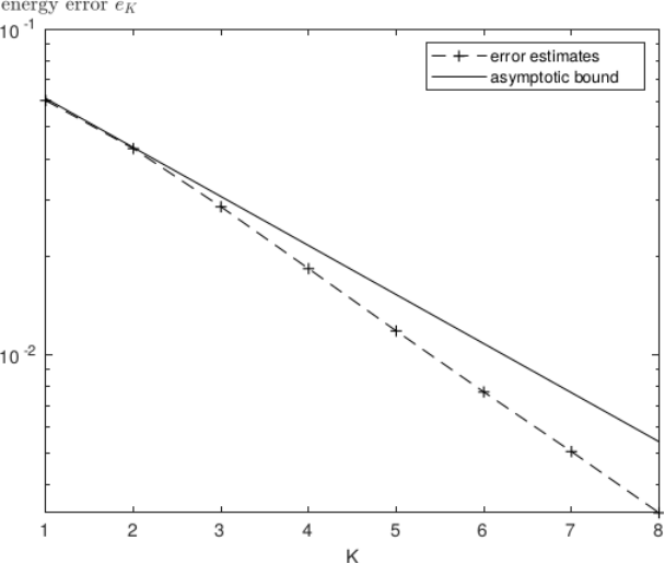
In case of the Cantor interface network (cf. Example 2.1) the solutions uKu_{K} of the level-KK interface Problem 2.3 for K∈ℕK\in\mathbb{N} converge exponentially to the solution uu of the fractal interface Problem 3.11 (cf. Remark 4.3). For a numerical illustration, we consider this example in d=2d=2 space dimensions with 𝔠=1\mathfrak{c}=1, f≡1f\equiv 1, A≡1A\equiv 1, and the geometrical parameter CK=2K−1C_{K}=2^{K-1}. Note that the ∥⋅∥\|\cdot\| norm in ℋ\mathcal{H} (cf. (25)) is identical with the energy norm induced by a⁡(⋅,⋅)a(\cdot,\cdot) (cf. (27)) in this instance.

Figure 4. Initial triangulation 𝒯(1)\mathcal{T}^{(1)}, uniform refinement 𝒯(2)\mathcal{T}^{(2)} together with the Cantor interface network Γ(K)\Gamma^{(K)} for K=1K=1, 22, and 88 in d=2d=2 space dimensions

The initial triangulation 𝒯(1)\mathcal{T}^{(1)} with h1=2−1h_{1}=2^{-1} is depicted in the left picture of Figure 4 (grey) together with the initial Cantor network Γ(1)\Gamma^{(1)} (black). Successive uniform refinement of 𝒯(1)\mathcal{T}^{(1)} provides the triangulations 𝒯(K)\mathcal{T}^{(K)} with hK=2−Kh_{K}=2^{-K} resolving the interfaces Γ(K)\Gamma^{(K)} on subsequent levels KK. The case K=2K=2 is illustrated in the middle while the right picture of Figure 4 shows the Cantor network Γ(8)\Gamma^{(8)}.

The linear systems associated with the corresponding finite element discretizations (39) on each level KK are solved directly. Exploiting

‖u−uK‖≤‖u−u9‖+‖u9−uK‖,K∈ℕ,\|u-u_{K}\|\leq\|u-u_{9}\|+\|u_{9}-u_{K}\|\;,\qquad K\in\mathbb{N}\;,

the fractal homogenization error is replaced by the heuristic error estimate

(40) eK=|u~10−u~9|+‖u~9−u~K‖,K=1,…,8.e_{K}=\|\tilde{u}_{10}-\tilde{u}_{9}\|+\|\tilde{u}_{9}-\tilde{u}_{K}\|\;,\qquad K=1,\dots,8\;.

The first term in (40) is intended to capture the error made by resolving a “large” but finite number of interfaces instead of infinitely many, while the second term aims at the additional contribution made by resolving only the actual “small” number of K=1,…,8K=1,\dots,8 levels.

Figure 5 shows the error estimates eKe_{K} over the levels KK (dotted line) together with the expected asymptotic bound of order (1+𝔠)−K(1+\mathfrak{c})^{-K} (solid line) for K=1,…,8K=1,\dots,8. Both curves have very similar slope which nicely confirms our theoretical findings. As ‖u−u9‖≥‖u10−u9‖\|u-u_{9}\|\geq\|u_{10}-u_{9}\| and ‖u~9−u~K‖=0\|\tilde{u}_{9}-\tilde{u}_{K}\|=0 for K=9K=9, we would expect that eKe_{K} underestimates the fractal homogenization error for increasing KK. This could explain the slight deviation from the expected asymptotic behavior.
Refer to caption
Figure 5. Exponential decay of fractal homogenization error

5.2. Fractal numerical homogenization

Aiming at an iterative solution of the discrete problems (39) with a convergence speed that is independent of the number of levels K∈ℕK\in\mathbb{N}, we now present a multilevel preconditioner in the spirit of [26, 27].

To this end, we introduce the sets of local patches

𝑸(k)={{𝑸¯} for k=1{𝝎x(k)⊂𝑸¯|x∈𝒩(k−1)} for k≥2\boldsymbol{Q}^{(k)}=\left\{\begin{array}[]{ccl}\{\overline{\boldsymbol{Q}}\}&\text{ for }&k=1\\ \left\{\boldsymbol{\omega}_{x}^{(k)}\subset\overline{\boldsymbol{Q}}\,|\;x\in\mathcal{N}^{(k-1)}\right\}&\text{ for }&k\geq 2\end{array}\right.

with 𝝎x(k)⊂𝑸¯\boldsymbol{\omega}_{x}^{(k)}\subset\overline{\boldsymbol{Q}} consisting of all simplices T∈𝒯(k−1)T\in\mathcal{T}^{(k-1)} with common vertex x∈𝒩(k−1)x\in\mathcal{N}^{(k-1)}. The decomposition of 𝑸\boldsymbol{Q} into patches 𝝎∈𝑸(k)\boldsymbol{\omega}\in\boldsymbol{Q}^{(k)} gives rise to the decomposition

(41) S(k)=∑𝝎∈𝑸(k)S𝝎(k),k∈ℕ,S^{(k)}=\sum_{\boldsymbol{\omega}\in\boldsymbol{Q}^{(k)}}S_{\boldsymbol{\omega}}^{(k)}\;,\qquad k\in\mathbb{N}\;,

into the local finite element spaces

S𝝎(k)={v∈S(k)|v|𝑸\int ​𝝎=0},ω∈𝑸(k).S_{\boldsymbol{\omega}}^{(k)}=\{v\in S^{(k)}\;|\;v|_{\boldsymbol{Q}\backslash\text{int }\boldsymbol{\omega}}=0\}\;,\qquad\omega\in\boldsymbol{Q}^{(k)}\;.

For each fixed K∈ℕK\in\mathbb{N}, this leads to the splitting

S(K)=∑k=1K∑𝝎∈𝑸(k)S𝝎(k)S^{(K)}=\sum_{k=1}^{K}\sum_{\boldsymbol{\omega}\in\boldsymbol{Q}^{(k)}}S_{\boldsymbol{\omega}}^{(k)}

and the corresponding multilevel preconditioner [35, 36]

(42) TK=∑k=0K∑𝝎∈𝑸(k)PS𝝎(k).T_{K}=\sum\limits_{k=0}^{K}\sum\limits_{\boldsymbol{\omega}\in\boldsymbol{Q}^{(k)}}P_{S_{\boldsymbol{\omega}}^{(k)}}.

with PV:S(K)⟶VP_{V}:S^{(K)}\longrightarrow V denoting the Ritz projection,

defined by

(43) a⁡(PV​w,v)=a⁡(w,v),∀v∈V.a(P_{V}w,v)=a(w,v),\quad\forall v\in V.

Note that the evaluation of each local projection PS𝝎(k)P_{S_{\boldsymbol{\omega}}^{(k)}} amounts to the solution of a (small) self-adjoint linear system on the patch 𝝎∈𝑸(k)\boldsymbol{\omega}\in\boldsymbol{Q}^{(k)}. Therefore, TKT_{K} can be regarded as a multilevel version of the classical block Jacobi preconditioner.

The analysis of upper bounds for the condition number of TKT_{K} as well as fractal counterparts of multiscale finite elements [25, 28] will be considered in a separate publication.

5.2.1. Cantor interface network

We consider the level-KK interface Problem 2.3 for the Cantor interface network with parameters, finite element discretization, and initial triangulation 𝒯(1)\mathcal{T}^{(1)} as previously described in subsection 5.1.

Let u~K(ν)\tilde{u}_{K}^{(\nu)}, ν∈ℕ\nu\in\mathbb{N}, denote the iterates of the preconditioned conjugate gradient method with preconditioner TKT_{K} given in (42) and initial iterate u~K(0)=u~0\tilde{u}_{K}^{(0)}=\tilde{u}_{0}. The corresponding algebraic error reduction factors

(44) ρK(ν)=‖u~K−u~K(ν)‖‖u~K−u~K(ν−1)‖\rho_{K}^{(\nu)}=\frac{\|\tilde{u}_{K}-\tilde{u}_{K}^{(\nu)}\|}{\|\tilde{u}_{K}-\tilde{u}_{K}^{(\nu-1)}\|}

of each iteration step are depicted in Figure 6 for ν=1,…,8\nu=1,\dots,8 together with their geometric average ρK\rho_{K} for K=5,…,9K=5,\dots,9. The averaged reduction factors ρK\rho_{K} seem to saturate with increasing level KK.

ν\nu K=5K=5 K=6K=6 K=7K=7 K=8K=8 K=9K=9
11 0.4790.479 0.4810.481 0.4810.481 0.4820.482 0.4820.482
22 0.4450.445 0.4640.464 0.4830.483 0.5000.500 0.5140.514
33 0.4530.453 0.4480.448 0.4420.442 0.4370.437 0.4390.439
44 0.4290.429 0.4520.452 0.4740.474 0.4930.493 0.5030.503
55 0.4510.451 0.4650.465 0.4680.468 0.4720.472 0.4770.477
66 0.4320.432 0.4440.444 0.4590.459 0.4770.477 0.4940.494
77 0.4470.447 0.4670.467 0.4630.463 0.4560.456 0.4550.455
88 0.4500.450 0.4830.483 0.4870.487 0.4890.489 0.4900.490
ρK\rho_{K} 0.4480.448 0.4630.463 0.4690.469 0.4750.475 0.4810.481
Figure 6. Algebraic error reduction factors for the Cantor interface network

In practical computations, it is sufficient to reduce the algebraic error ‖u~K−u~K(ν)‖\|\tilde{u}_{K}-\tilde{u}_{K}^{(\nu)}\| up to discretization accuracy ‖uK−u~K‖\|u_{K}-\tilde{u}_{K}\|. Galerkin orthogonality implies

‖u~K+1−u~K‖2+‖u−u~K+1‖2=‖u−u~K‖2.\|\tilde{u}_{K+1}-\tilde{u}_{K}\|^{2}+\|u-\tilde{u}_{K+1}\|^{2}=\|u-\tilde{u}_{K}\|^{2}\;.

We utilize the stopping criterion

(45) ‖u~K−u~K(ν0)‖≤‖u~K+1−u~K‖≤‖u−u~K‖\|\tilde{u}_{K}-\tilde{u}_{K}^{(\nu_{0})}\|\leq\|\tilde{u}_{K+1}-\tilde{u}_{K}\|\leq\|u-\tilde{u}_{K}\|

provided by the resulting lower bound for the discretization error and the final iterate on the preceding level K−1K-1 as the initial iterate on the actual level KK (nested iteration). Then, only ν0=1\nu_{0}=1 step of the preconditioned conjugate gradient iteration is sufficient to provide an approximation u~K(ν0)\tilde{u}_{K}^{(\nu_{0})} of u~K\tilde{u}_{K} with discretization accuracy for all K=2,…,9K=2,\dots,9.

5.2.2. Layered interfaces

We consider the level-KK interface Problem 2.3 in d=2d=2 space dimensions with parameters 𝔠=1\mathfrak{c}=1, f≡1f\equiv 1, A≡1A\equiv 1, and non-intersecting interfaces Γk⊂𝑸=(0,1)2\Gamma_{k}\subset\boldsymbol{Q}=(0,1)^{2} described as follows. Figure 7 shows the initial triangulation 𝒯(1)\mathcal{T}^{(1)} (grey) with h1=2−4h_{1}=2^{-4} together with the 3 macro interfaces forming Γ(1)\Gamma^{(1)}. Again, 𝒯(k)\mathcal{T}^{(k)} is obtained by uniform refinement of 𝒯(1)\mathcal{T}^{(1)} and Γk=Γ(K)\Γ(K−1)\Gamma_{k}=\Gamma^{(K)}\backslash\Gamma^{(K-1)} is composed of 6 randomly selected, non-intersecting polygons consisting of edges of triangles T∈𝒯(K)T\in\mathcal{T}^{(K)} one above and one below each macro interface from Γ(1)\Gamma^{(1)}. For K=2K=2, this is illustrated in the middle picture of Figure 7. Note that at most CK=2K−1C_{K}=2^{K}-1 interfaces are cut by any straight line through 𝑸\boldsymbol{Q}. The final interface Γ(6)\Gamma^{(6)} is displayed in the right picture.

Figure 7. Initial triangulation 𝒯(1)\mathcal{T}^{(1)}, uniform refinement 𝒯(2)\mathcal{T}^{(2)} together with the layered interface network Γ(K)\Gamma^{(K)} for K=1K=1, 22, and 66
ν\nu K=2K=2 K=3K=3 K=4K=4 K=5K=5 K=6K=6
11 0.3030.303 0.3770.377 0.3760.376 0.3920.392 0.4230.423
22 0.1770.177 0.4310.431 0.4730.473 0.4960.496 0.5230.523
33 0.3290.329 0.3160.316 0.4180.418 0.4920.492 0.5420.542
44 0.3720.372 0.4040.404 0.4050.405 0.4970.497 0.5170.517
55 0.2470.247 0.4090.409 0.5010.501 0.5030.503 0.5250.525
66 0.3290.329 0.4050.405 0.4210.421 0.4970.497 0.5330.533
77 0.3660.366 0.3620.362 0.4580.458 0.480.488 0.5390.539
88 0.3280.328 0.4400.440 0.4260.426 0.4970.497 0.5270.527
ρK\rho_{K} 0.2990.299 0.3910.391 0.4330.433 0.4810.481 0.5150.515
Figure 8. Algebraic error reduction factors for the layered interface network

As in Subsection 5.2.1, we consider the conjugate gradient iteration with the multilevel preconditioner defined in (42) and initial iterate uK(0)=u~0u_{K}^{(0)}=\tilde{u}_{0} for K=2,…,6K=2,\dots,6. Figure 8 shows the algebraic error reduction factors ρK(ν)\rho_{K}^{(\nu)} defined in (44), together with their geometric average ρK\rho_{K}. The averaged reduction factors ρK\rho_{K} are slightly increasing with increasing level KK.

If nested iteration is applied, only one iteration step is needed to reach discretization accuracy according to the stopping criterion (45) in Subsection 5.2.1.

References

  • [1] Grégoire Allaire. Homogenization and two-scale convergence. SIAM Journal on Mathematical Analysis, 23(6):1482–1518, 1992.
  • [2] Grégoire Allaire and Marc Briane. Multiscale convergence and reiterated homogenisation. Proceedings of the Royal Society of Edinburgh Section A: Mathematics, 126(2):297–342, 1996.
  • [3] Scott Armstrong, Tuomo Kuusi, and Jean-Christophe Mourrat. Quantitative stochastic homogenization and large-scale regularity. arXiv preprint arXiv:1705.05300, 2017.
  • [4] Scott N. Armstrong and Charles K. Smart. Quantitative stochastic homogenization of elliptic equations in nondivergence form. Archive for Rational Mechanics and Analysis, 214(3):867–911, 2014.
  • [5] Léonardo Baffico, Céline Grandmont, Yvon Maday, and Axel Osses. Homogenization of elastic media with gaseous inclusions. Multiscale Modeling & Simulation, 7(1):432–465, 2008.
  • [6] Randolph E. Bank, Andrew H. Sherman, and Alan Weiser. Some refinement algorithms and data structures for regular local mesh refinement. Scientific Computing, Applications of Mathematics and Computing to the Physical Sciences, 1:3–17, 1983.
  • [7] Yehuda Ben-Zion and Charles G. Sammis. Characterization of fault zones. Pure and Applied Geophysics, 160(3-4):677–715, 2003.
  • [8] Jürgen Bey. Simplicial grid refinement: on Freudenthal’s algorithm and the optimal number of congruence classes. Numerische Mathematik, 85(1):1–29, 2000.
  • [9] Eduardo Casas and Luis Alberto Fernández. A green’s formula for quasilinear elliptic operators. Journal of mathematical analysis and applications, 142(1):62–73, 1989.
  • [10] Paul Cazeaux, Céline Grandmont, and Yvon Maday. Homogenization of a model for the propagation of sound in the lungs. Multiscale Modeling & Simulation, 13(1):43–71, 2015.
  • [11] Doina Cioranescu, Alain Damlamian, Patrizia Donato, Georges Griso, and Rachad Zaki. The periodic unfolding method in domains with holes. SIAM Journal on Mathematical Analysis, 44(2):718–760, 2012.
  • [12] Doina Cioranescu, Alain Damlamian, and Julia Orlik. Homogenization via unfolding in periodic elasticity with contact on closed and open cracks. Asymptotic Analysis, 82(3-4):201–232, 2013.
  • [13] Patrizia Donato and Sara Monsurro. Homogenization of two heat conductors with an interfacial contact resistance. Analysis and Applications, 2(03):247–273, 2004.
  • [14] Yalchin Efendiev and Thomas Y. Hou. Multiscale Finite Element Methods: Theory and Applications, volume 4. Springer Science & Business Media, 2009.
  • [15] Lawrence C. Evans. Partial Differential Equations. American Mathematical Society, 1998.
  • [16] Xiang Gao and Kelin Wang. Strength of stick-slip and creeping subduction megathrusts from heat flow observations. Science, 345(6200):1038–1041, 2014.
  • [17] Antoine Gloria, Stefan Neukamm, and Felix Otto. An optimal quantitative two-scale expansion in stochastic homogenization of discrete elliptic equations. ESAIM: Mathematical Modelling and Numerical Analysis, 48(2):325–346, 2014.
  • [18] Georges Griso. Error estimate and unfolding for periodic homogenization. Asymptotic Analysis, 40(3, 4):269–286, 2004.
  • [19] Isabelle Gruais and Dan Poliševski. Heat transfer models for two-component media with interfacial jump. Applicable Analysis, 96(2):247–260, 2017.
  • [20] Martin Heida. An extension of the stochastic two-scale convergence method and application. Asymptotic Analysis, 72(1-2):1–30, 2011.
  • [21] Martin Heida. Stochastic homogenization of heat transfer in polycrystals with nonlinear contact conductivities. Applicable Analysis, 91(7):1243–1264, 2012.
  • [22] Ulrich Hornung. Homogenization and Porous Media, volume 6. Springer Science & Business Media, 2012.
  • [23] Hans-Karl Hummel. Homogenization of Periodic and Random Multidimensional Microstructures. PhD thesis, Technische Universität Bergakademie Freiberg, 1999.
  • [24] Vasilii Vasil’evich Jikov, Sergei M. Kozlov, and Olga Arsen’evna Oleĭnik. Homogenization of Differential Operators and Integral Functionals. Springer-Verlag, Berlin, 1994.
  • [25] Ralf Kornhuber, Daniel Peterseim, and Harry Yserentant. An analysis of a class of variational multiscale methods based on subspace decomposition. Mathematics of Computation, 87(314):2765–2774, 2018.
  • [26] Ralf Kornhuber, Joscha Podlesny, and Harry Yserentant. Direct and iterative methods for numerical homogenization. In Chang-Ock Lee, Xiao-Chuan Cai, David E. Keyes, Hyea Hyun Kim, Axel Klawonn, Eun-Jae Park, and Olof B. Widlund, editors, Domain Decomposition Methods in Science and Engineering XXIII, pages 217–225. Springer International Publishing, 2017.
  • [27] Ralf Kornhuber and Harry Yserentant. Numerical homogenization of elliptic multiscale problems by subspace decomposition. Multiscale Modeling and Simulation, 14(3):1017–1036, 2016.
  • [28] Axel Målqvist and Daniel Peterseim. Localization of elliptic multiscale problems. Mathematics of Computation, 83(290):2583–2603, 2014.
  • [29] Umberto Mosco and Maria Agostina Vivaldi. Thin fractal fibers. Mathematical Methods in the Applied Sciences, 36(15):2048–2068, 2013.
  • [30] Hiroyuki Nagahama and Kyoko Yoshii. Scaling laws of fragmentation. In Fractals and Dynamic Systems in Geoscience, pages 25–36. Springer, 1994.
  • [31] Onno Oncken, David Boutelier, Georg Dresen, and Kerstin Schemmann. Strain accumulation controls failure of a plate boundary zone: Linking deformation of the central andes and lithosphere mechanics. Geochemistry, Geophysics, Geosystems, 13(12), 2012.
  • [32] Alfio Quarteroni and Alberto Valli. Domain decomposition methods for partial differential equations. Oxford University Press, 1999.
  • [33] Charles G. Sammis, Robert H. Osborne, J. Lawford Anderson, Mavonwe Banerdt, and Patricia White. Self-similar cataclasis in the formation of fault gouge. Pure and Applied Geophysics, 124(1):53–78, 1986.
  • [34] Donald L. Turcotte. Crustal deformation and fractals, a review. In Jörn H. Kruhl, editor, Fractals and Dynamic Systems in Geoscience, pages 7–23. Springer, 1994.
  • [35] Jinchao Xu. Iterative methods by space decomposition and subspace correction. SIAM Review, 34(4):581–613, 1992.
  • [36] Harry Yserentant. Old and new convergence proofs for multigrid methods. Acta Numerica, 2:285–326, 1993.
  • [37] Vasili Vasil’evich Zhikov and Aleksandr L. Pyatnitskiĭ. Homogenization of random singular structures and random measures. Izvestiya Rossiĭskaya Akademiya Nauk. Seriya Matematicheskaya, 70(1):23–74, 2006.