Coarse Grained Parallel Selection

Laurence Boxer ^†^†thanks: Department of Computer and Information Sciences, Niagara University, Niagara University, NY 14109, USA; and Department of Computer Science and Engineering, State University of New York at Buffalo. E-mail: boxer@niagara.edu

Abstract

Several efficient, but non-optimal, solutions to the Selection Problem on coarse grained parallel computers have appeared in the literature. We consider the example of the Saukas-Song algorithm; we analyze it without expressing the running time in terms of communication rounds. This shows that while in the best case the Saukas-Song algorithm runs in asymptotically optimal time, in general it does not. We propose another algorithm for coarse grained selection that has optimal expected running time.

Key words and phrases: selection problem, coarse grained multicomputer, uniform distribution, Chebyshev’s inequality

1 Introduction

Several algorithms for solution of the Selection Problem on coarse grained parallel computers, including those of [1, 2, 7, 8, 9, 13, 14], have been proposed. Among these are algorithms that are efficient but not asymptotically optimal.

We consider for example the paper [13], by Saukas and Song, who present the analysis of their algorithm in terms of the amount of time spent in local sequential operations and the number of communications rounds. In the current paper, we replace analysis of the number of communications rounds with an analysis of their running times, giving us asymptotic analysis of the running time for the entire algorithm. This lets us show that although the Saukas-Song algorithm is efficient, it is not optimal. We show that an algorithm for coarse grained parallel selection that is not asymptotically optimal can be modified to obtain an algorithm with asymptotically optimal expected running time.

2 Preliminaries

2.1 Model of Computation

Material in this section is quoted or paraphrased from [5].

The coarse grained multicomputer model, or $CGM(n,p)$ , considered in this paper, has $p$ processors with $\Omega(n/p)$ local memory apiece - i.e., each processor has $\Omega(n/p)$ memory cells of $\Theta(\log n)$ bits apiece. The processors may be connected to some (arbitrary) interconnection network (such as a mesh, hypercube, or fat tree) or may share global memory. A processor may exchange messages of $O(\log n)$ bits with any immediate neighbor in constant time. In determining time complexities, we consider both local computation time and interprocessor communication time, in standard fashion. The term “coarse grained” means that the size $\Omega(n/p)$ of each processor’s memory is “considerably larger” than $\Theta(1)$ ; by convention, we usually assume $n/p\geq p$ (equivalently, $n\geq p^{2}$ ), but will occasionally assume other relations between $n$ and $p$ , typically such that each processor has at least enough local memory to store the ID number of every other processor. For more information on this model and associated operations, see [6].

2.2 Terminology and notation

We say an array $list[1\ldots n]$ is evenly distributed in a $CGM(n,p)$ if each processor has $\Theta(n/p)$ members of the array.

We use the notation $\#X$ for the number of members of the set $X$ .

2.3 Semigroup operations

Let $X=\{x_{j}\}_{j=1}^{n}$ be a set of data values and let $\circ$ be a binary operation on $X$ . A semigroup operation computes $x_{1}\circ x_{2}\circ\ldots\circ x_{n}$ . Examples of such operations include sum, average, min, and max.

Theorem 2.1.

[4] Let $X=\{x_{j}\}_{j=1}^{n}$ be a set of data values distributed $\Theta(n/p)$ per processor in a $CGM(n,p)$ . Then the semigroup computation of $x_{1}\circ x_{2}\circ\ldots\circ x_{n}$ can be performed in $\Theta(n/p)$ time. At the end of this algorithm, all processors hold the value of $x_{1}\circ\ldots\circ x_{n}$ . $\Box$

2.4 Data movement operations

In the literature of CGM algorithms, many papers, including [13], analyze an algorithm by combining the running time of sequential computations with the number of communications rounds. A communications round is described in [13] as an operation in which each processor of a $CGM(n,p)$ can exchange $O(n/p)$ data with other processors.

However, this definition does not lead to a clear understanding of the asymptotic running time of a CGM algorithm. E.g., a communication round could require a processor to send $\Theta(1)$ data to a neighboring processor, which can be done in $\Theta(1)$ time; or, a communication round could require communication of $\Theta(1)$ data between diametrically opposite processors of a linear array, which requires $\Theta(p)$ time.

Further, there is a sense in which the notion of a communication round is not well defined. Consider again the example of communication of $\Theta(1)$ data between diametrically opposite processors $P_{1},P_{p}$ of a linear array in which the processors $P_{i}$ are indexed sequentially, i.e., $P_{1}$ is adjacent to $P_{2}$ and $P_{i}$ is adjacent to $P_{i-1}$ and to $P_{i+1}$ for $1<i<p$ . This communication can be regarded as a single communication round according to the description given above; or as $p-1$ communication rounds, in the $i^{th}$ of which processor $P_{i}$ sends $\Theta(1)$ data to processor $P_{i+1}$ , $1\leq i<p$ .

Now that more is known about the running times of communications operations in CGM than when [13] appeared, we can fully analyze the running time of the algorithm. In the remainder of this section, we discuss running times of communications operations used in the Saukas-Song algorithm.

Theorem 2.2.

[4] A unit of data can be broadcast from one processor to all other processors of a $CGM(n,p)$ in $O(p)$ time. $\Box$

Let $S$ be a set of data values distributed, not necessarily evenly, among the processors of a parallel computer. A gather operation results in a copy of $S$ being in a single processor $P_{i}$ , and we say $S$ has been gathered to $P_{i}$ [4, 11]. We have the following.

Theorem 2.3.

[4] Let $S$ be a nonempty set of $N$ elementary data values distributed among the processors of $G$ , a $CGM(n,p)$ , such that $N=\Omega(p)$ and $N=O(n/p)$ . Then $S$ can be gathered to any processor of $G$ in $\Theta(N)$ time. $\Box$

3 Analysis of the Saukas-Song algorithm

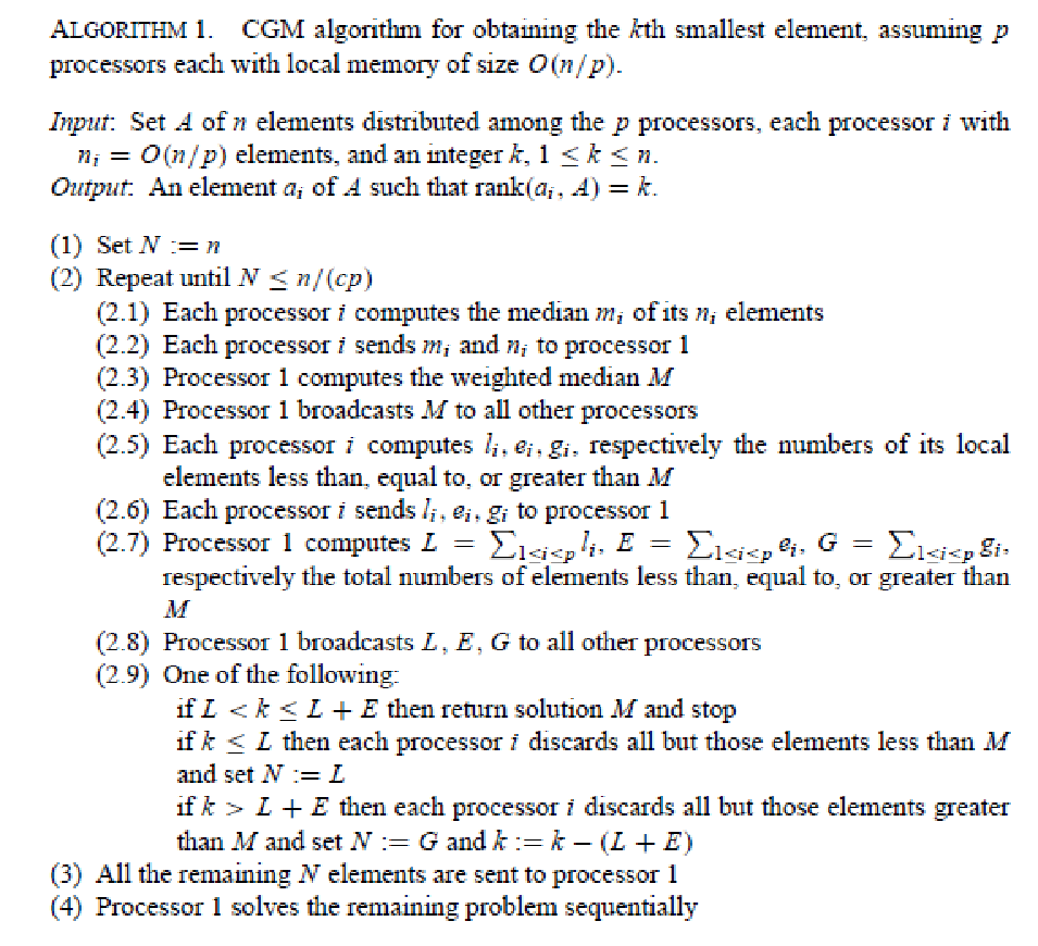
The algorithm of [13] is given in Figure 1. Note it is assumed in [13] that $n>p^{2}\log p$ . We will refer to the steps of the algorithm as labeled in this figure. For convenience, we will take $c=1$ in step (2).

Refer to caption — Figure 1: The Saukas-Song algorithm of [13]

Theorem 3.1.

[13] After each performance of the body of the loop in step (2), the number of elements remaining under consideration is reduced by at least one quarter. $\Box$

Corollary 3.2.

The number of performances of the body of the loop in step (2) is $O(\log p)$ .

Proof.

It follows from Theorem 3.1 that after $k$ performances of the body of the loop, the number of elements remaining under consideration is at most $(3/4)^{k}n$ . Since step (2) terminates in the worst case when the number of elements remaining under consideration is at most $n/p$ , termination requires, in the worst case, $(3/4)^{k}n\leq n/p$ , or $p\leq(4/3)^{k}$ . The smallest integer $k$ satisfying this inequality must therefore satisfy $k=\Theta(\log p)$ . Since the loop could terminate after as little as 1 performance of its body, the assertion follows. ∎

Theorem 3.3.

Assume $n>p^{2}\log_{2}p$ . The Saukas-Song algorithm for the Selection Problem runs in $\Theta(\frac{n\log p}{p})$ time on a $CGM(n,p)$ in the worst case. In the best case, the running time is $\Theta(n/p)$ . We may assume that at the end of the algorithm, every processor has the solution to the Selection Problem.

Proof.

We give the following argument.

•

Clearly, step (1) executes in $\Theta(1)$ time.
•
We analyze step (2) as follows.
1. 1.
  
  Step (2.1) is executed by a linear-time sequential algorithm [3, 10]. As Saukas and Song observed, our algorithm does not guarantee that the data being considered are evenly distributed among the processors throughout the repetitions of the loop body. In the worst case, some processor could have $\Theta(n/p)$ data in each iteration of the loop body. Therefore, this step executes in worst case $\Theta(n/p)$ time.
2. 2.
  
  Step (2.2) is performed by a gather operation. By Theorem 2.3, this can be done in $\Theta(p)$ time.
3. 3.
  
  Step (2.3) is performed in $\Theta(p)$ time by a linear-time sequential algorithm.
4. 4.
  
  Step (2.4) is performed by a broadcast operation. By Theorem 2.2, this requires $O(p)$ time.
5. 5.
  
  Step (2.5) is performed by sequential semigroup (counting) operations performed by all processors in parallel, in linear time [10]. As noted above, in the worst case a processor could have $\Theta(n/p)$ data in each iteration of the loop body. Therefore, this step executes in $O(n/p)$ time.
6. 6.
  
  Step (2.6) is performed by a gather operation. As above, this can be done in $O(p)$ time.
7. 7.
  
  Step (2.7) is executed by semigroup operations in $\Theta(p)$ time.
8. 8.
  
  Step (2.8) is performed by a broadcast operation in $O(p)$ time.
9. 9.
  
  In the worst case, Step (2.9) requires each processor $P_{i}$ to discard $O(n/p)$ data items. This can be done as follows. In parallel, each processor $P_{i}$ rearranges its share of the data so that the undiscarded items are at the beginning of the segment of (a copy of) $list$ stored in $P_{i}$ , using a sequential prefix operation in $O(n/p)$ time.
Thus, the worst case time required for one performance of the body of the loop of step (2) is $\Theta(n/p+p)=\Theta(n/p)$ . By Corollary 3.2, the loop executes its body $\Theta(\log p)$ times in the worst case. Thus, the loop executes all performances of its body in worst case $\Theta(\frac{n\log p}{p})$ time.
•

Step (3) is performed by a gather operation. Since we now have $N\leq n/p$ , Theorem 2.3 implies this is done in $O(n/p)$ time.
•

Step (4) uses a linear time sequential algorithm to solve the problem in $\Theta(N)=O(n/p)$ time.
•

Additionally, processor 1 can broadcast its solution to all other processors. By Theorem 2.2, this requires $O(p)$ time.

Thus, the algorithm uses worst case $\Theta(\frac{n\log p}{p})$ time.

In the best case, the loop of step (2) executes its body once, when in step (2.9) it is found that $L<k\leq L+E$ . In this case, step (2) executes in $\Theta(n/p)$ time, and the algorithm executes in $\Theta(n/p)$ time. ∎

4 Expected-optimal selection algorithms

In this section, we consider modification of algorithms for the selection problem on coarse grained multicomputers, based on the familiar idea that if we know the distribution of data values, then, with high probability, we can estimate the desired value to within a small interval and, in so doing, eliminate (with high probability) most of the data values from consideration as possible solutions. In the following, we assume the data values are uniformly distributed over some interval.

4.1 Useful formulas from probability and statistics

We use the notation $Pr[H]$ for the probability of the event $H$ , and $Pr[D|C]$ for the conditional probability of the event $D$ given that $C$ occurs. We use the notation $\overline{H}$ for “not $H$ ”.

Let $X_{(k)}$ be a random variable for the $k^{th}$ smallest member of a set $\{x_{i}\}_{i=1}^{n}$ of data points uniformly distributed over the interval $[0,1]$ . Then the expected value $E(X_{(k)})$ and variance $V(X_{(k)})$ of $X_{(k)}$ are given [12] by the following.

E(X_{(k)})=k/(n+1)

(1)

V(X_{(k)})=\frac{k(n+1-k)}{(n+1)^{2}(n+2)}

(2)

We recall also Chebyshev’s Inequality:

Theorem 4.1.

[12] Let $y$ be a random variable with expected value $E(y)=\mu$ and variance $V(y)=v$ . Then, for any $t>0$ ,

Pr\left[|y-\mu|>t\right]\leq\frac{v}{t^{2}}.

(3)

4.2 Algorithm

The solution to the Selection Problem proposed below assumes an existing solution $F$ , such as the Saukas-Song algorithm, and therefore must satisfy the same or a stronger restriction on the number of processors as the solution $F$ . We assume there is a function $B_{F}(p)$ associated with $F$ such that $p^{2}\leq B_{F}(p)\leq n$ . E.g., for the Saukas-Song algorithm we take $B_{F}(p)=p^{2}\log_{2}p$ . We will use a slightly stricter limitation,

\mbox{For some }w>2,~B_{F}(p)=p^{w}\leq n;\mbox{ equivalently, }n/p\geq n^{1-1/w}.

(4)

The latter inequality derives from the former, since

p^{w}\leq n\Leftrightarrow p\leq n^{1/w}\Leftrightarrow n/p\geq\frac{n}{n^{1/w}}=n^{1-1/w}.

Note this also implies

p\leq n^{1/w}\leq\mbox{ ~~~(since }w>2)~~~~n^{1-1/w}\leq n/p.

(5)

We use the fact that the real function $G(x)=x(n-x)$ is maximized at $x=n/2$ , from which it follows that

x(n-x)\leq G(n/2)=n^{2}/4.

(6)

Our algorithm has an asymptotically optimal expected running time, $\Theta(n/p)$ , and its worst case running time is that of $F$ .

Theorem 4.2.

Let $F$ be an algorithm to solve the Selection Problem on a $CGM(n,p)$ , where $p$ is restricted by (4). Suppose $F$ has running time $R_{F}(n,p)=O(\frac{n\log p}{p})$ (e.g., the Saukus-Song algorithm). Suppose we are given a set $A$ of $n$ elements distributed $\Theta(n/p)$ per processor among the processors of a $CGM(n,p)$ and an integer $k$ such that $1\leq k\leq n$ . Assume the key values of the elements of $A$ are uniformly distributed over an interval $[u,v]$ . Then the $k^{th}$ smallest member of $A$ can be found in expected $\Theta(n/p)$ time. The worst case running time is $\Theta(R_{F}(n,p))$ .

Proof.

Without loss of generality, $[u,v]=[0,1]$ .

If the values of $n$ and $p$ are not known, they can be computed and made know to all processors via semigroup (counting) operations. By Theorem 2.1, this can be done in $\Theta(n/p)$ time.

Let $c$ be a small positive integer.

If $k\leq c$ then we can find the desired result by $k$ performances of a minimum computation. I.e., we do the following.

For	$i=1$ to $k$
	Find an element $a_{j}\in A$ such that $a_{j}=\min\{a\in A\}$ .
	If $i=k$	then the desired result is $a_{j}$ ; else set $A=A\setminus\{a_{j}\}$ .
End For

By Theorem 2.1 and (5), the For loop executes in $\Theta(n/p)$ time, and by Theorem 2.2, the result can be distributed to all processors in $O(p)$ time. By (5), the case $k\leq c$ is solved in $\Theta(n/p)$ time.

If $k\geq n-c$ , then we do the following.

For	$i=n$ to $k$ step $-1$
	Find an element $a_{j}\in A$ such that $a_{j}=\max\{a\in A\}$ .
	If $i=k$ then the desired result is $a_{j}$ ; else set $A=A\setminus\{a_{j}\}$ .
End For

By Theorem 2.1 and (5), the For loop executes in $\Theta(n/p)$ time, and by Theorem 2.2, the result can be distributed to all processors in $O(p)$ time. By (5), the case $k\geq n-c$ is solved in $\Theta(n/p)$ time.

The remaining case is $c<k<n-c$ . Let

\varepsilon=n^{-1/3}.

(7)

Proceed as follows.

•

In $\Theta(1)$ time, each processor computes

$U=\max\{0,\frac{k}{n+1}-\varepsilon\}$ (8)

and

$V=\min\{1,\frac{k}{n+1}+\varepsilon\}.$ (9)
•
In parallel, each processor $P_{j}$ scans its portion of the data set $A=\{x_{i}\}_{i=1}^{n}$ to determine
- –
  
  $S_{j}$ , the number of elements of $A$ in $P_{j}$ that are less than U; and
- –
  
  $M_{j}$ , the number of elements of $A$ in $P_{j}$ that are in $[U,V]$ .
This can be done in $\Theta(n/p)$ time.
•

Gather the $S_{j}$ values to one processor and compute their sum, $S=\sum_{j=1}^{p}S_{j}$ . Similarly, gather the $M_{j}$ values to one processor and compute their sum, $M=\sum_{j=1}^{p}M_{j}$ . Broadcast the values $S,M$ to all processors. From Theorems 2.3 and 2.2, we conclude that all this can be done in $\Theta(p)$ time.
•

If $S<k\leq S+M$ , then we have $X_{(k)}\in[U,V]$ ; and if further we have $M\leq n/p$ then the $k^{th}$ smallest member of $A$ is the $(k-S)^{th}$ smallest member of the subset $M^{\prime}$ of $A$ consisting of members of $A\cap[U,V]$ . Since $\#M^{\prime}=M$ , we can gather the elements of $M^{\prime}$ to one processor in $\Theta(M)=O(n/p)$ time according to Theorem 2.3, and have that processor sequentially find the $(k-S)^{th}$ smallest member of $M^{\prime}$ in $\Theta(M)=O(n/p)$ time, and broadcast the result to all processors in $O(p)$ time.

Thus, if this case is realized, the running time of the algorithm is $\Theta(n/p)$ , which is asymptotically optimal, since the optimal sequential running time for solving the Selection Problem is $\Theta(n)$ .
This leaves the following cases to be considered.
- –
  
  If $S<k\leq S+M$ and $M>n/p$ , then apply the algorithm $F$ to finding the $(k-S)^{th}$ smallest member of $T_{1}=\{x\in A\,|\,S<x<S+M\}$ . In the worst case, $\#T_{1}=\Theta(n)$ and the asymptotic running time of this step is $R_{F}(n,p)$ .
- –
  
  If $k\leq S$ then apply the algorithm $F$ to finding the $k^{th}$ smallest member of $T_{2}=\{x\in A\,|\,x<U\}$ . In the worst case, $\#T_{2}=\Theta(n)$ and the asymptotic running time of this step is $R_{F}(n,p)$ .
- –
  
  Otherwise, $k>S+M$ and the desired value is the $(k-(S+M))^{th}$ smallest member of $T_{3}=\{x\in A\,|\,x>V\}$ . Use the algorithm $F$ to find the $(k-(S+M))^{th}$ smallest member of $T_{3}$ . In the worst case, $\#T_{3}=\Theta(n)$ and the asymptotic running time is $R_{F}(n,p)$ .

It remains for us to show that $\Theta(n/p)$ is the expected running time of the algorithm.

Let $C$ be the event

C=[U\leq X_{(k)}\leq V].

The event complementary to $C$ is

\overline{C}=\left[X_{(k)}<U\right]\cup\left[V<X_{(k)}\right].

By (8) and (9), $\overline{C}\subset\left[|X_{(k)}-E(X_{(k)})|>\varepsilon\right]$ , so by (1), (2), Theorem 4.1, (6), and (7),

Pr[\overline{C}]\leq\frac{\frac{k(n+1-k)}{(n+1)^{2}(n+2)}}{\varepsilon^{2}}\leq\frac{(n+1)^{2}}{4\varepsilon^{2}(n+1)^{2}(n+2)}=O(n^{-1/3}).

(10)

Therefore,

\lim_{n\to\infty}Pr[C]=1.

(11)

Let

D=\left[\#\{x\in A\,|\,U\leq x\leq v\}\leq\frac{n}{2p}\right].

Notice

C\cap D\mbox{ is a subset of the set of occurrences for which we do not run }F.

(12)

We have

\overline{D}=\left[\#\{x\in A\,|\,U\leq x\leq V\}>\frac{n}{2p}\right].

We consider the following cases.

•

Suppose $0<U$ and $V<1$ . Then

[\overline{D}|C]\subset[X_{(k-\frac{n}{4p})}>U]\,\cup\,[X_{(k+\frac{n}{4p})}<V]=

\left[X_{(k-\frac{n}{4p})}-E(X_{(k-\frac{n}{4p})})>U-E(X_{(k-\frac{n}{4p})})\right]\,\cup\,\left[E(X_{(k+\frac{n}{4p})})-V<E(X_{(k+\frac{n}{4p})})-X_{(k+\frac{n}{4p})}\right]

\subset\left[|X_{(k-\frac{n}{4p})}-E(X_{(k-\frac{n}{4p})})|>U-\frac{k-\frac{n}{4p}}{n+1}\right]\,\cup\,\left[\frac{k+\frac{n}{4p}}{n+1}-V<|X_{(k+\frac{n}{4p})}-E(X_{(k+\frac{n}{4p})})|\right].

For large $n$ , it follows from (4), (7), (8) and (9) that

U-\frac{k-\frac{n}{4p}}{n+1}=\frac{n}{4p(n+1)}-\ n^{-1/3}=\frac{k+\frac{n}{4p}}{n+1}-V>0,

Therefore, Theorem 4.1 yields

Pr[\overline{D}|C]\leq\frac{(k-\frac{n}{4p})(n+1-(k-\frac{n}{4p}))}{(n+1)^{2}(n+2)(U-\frac{k-\frac{n}{4p}}{n+1})^{2}}+\frac{(k+\frac{n}{4p})(n+1-(k+\frac{n}{4p}))}{(n+1)^{2}(n+2)(\frac{k+\frac{n}{4p}}{n+1}-V)^{2}}\leq

(by (6))

\frac{(n+1)^{2}}{4(n+1)^{2}(n+2)\left(\frac{n}{4p(n+1)}-\ n^{-1/3}\right)^{2}}+\frac{(n+1)^{2}}{4(n+1)^{2}(n+2)\left(\frac{n}{4p(n+1)}-n^{-1/3}\right)^{2}}

=\frac{2}{4(n+2)\left(\frac{n}{4p(n+1)}-n^{-1/3}\right)^{2}}<~~~\mbox{ (by (\ref{processorRestriction})) }~~~\frac{1}{2(n+2)\left(\frac{n^{1-1/w}}{4(n+1)}-n^{-1/3}\right)^{2}}

=O\left(n^{-(1-2/w)}\right).

•

If $U=0$ , then by (8), $\frac{k}{n+1}\leq\varepsilon$ , so by (7) and (9), $V\leq 2\varepsilon$ .

\overline{D}=\left[\#\{x\in A\,|\,x\leq V\}>\frac{n}{2p}\right]=\left[X_{(\frac{n}{2p}+1)}\leq V\right]\subset\left[X_{(\frac{n}{2p}+1)}\leq 2\varepsilon\right]=

\left[E(X_{(\frac{n}{2p}+1)})-2\varepsilon\leq E(X_{(\frac{n}{2p}+1)})-X_{(\frac{n}{2p}+1)}\right]\subset

\left[E(X_{(\frac{n}{2p}+1)})-2\varepsilon\leq|E(X_{(\frac{n}{2p}+1)})-X_{(\frac{n}{2p}+1)}|\right].

Since we have

E(X_{(\frac{n}{2p}+1)})-2\varepsilon=\frac{(\frac{n}{2p}+1)}{n+1}-2n^{-1/3}\geq\mbox{~~~(by (\ref{processorRestriction}))}

\frac{(\frac{n^{1/2}}{2}+1)}{n+1}-2n^{-1/3}=\Theta(n^{-1/2}),

therefore, for large $n$ , $E(X_{(\frac{n}{2p}+1)})-2\varepsilon>0$ , so by Theorem 4.1 we have

Pr[\overline{D}]\leq Pr\left[E(X_{(\frac{n}{2p}+1)})-2\varepsilon\leq|E(X_{(\frac{n}{2p}+1)})-X_{(\frac{n}{2p}+1)}|\right]\leq

\frac{(\frac{\frac{n}{2p}+1}{n+1})(n+1-(\frac{\frac{n}{2p}+1}{n+1}))}{(n+1)^{2}(n+2)\left(\frac{(\frac{n}{2p}+1)}{n+1}-2n^{-1/3}\right)^{2}}.

By (6), the numerator is at most $(n+1)^{2}/4$ , so

Pr[\overline{D}]\leq\frac{1}{4(n+2)\left(\frac{(\frac{n}{2p}+1)}{n+1}-2n^{-1/3}\right)^{2}}

\mbox{ (by (\ref{processorRestriction})) }~~~\frac{1}{4(n+2)\left(\frac{(\frac{n^{1-1/w}}{2}+1)}{n+1}-2n^{-1/3}\right)^{2}}=O\left(n^{-(1-2/w)}\right).

Hence

Pr[\overline{D}|C]=Pr[C\cap\overline{D}]/Pr[C]\leq Pr[\overline{D}]/Pr[C]=O\left(\frac{n^{-(1-2/w)}}{1}\right)=

O\left(n^{-(1-2/w)}\right).

•

The case $V=1$ is symmetric with the case $U=0$ and similarly produces the result $Pr[\overline{D}|C]=O\left(n^{-(1-2/w)}\right)$ .

Thus, in all cases,

Pr[\overline{D}|C]=O\left(n^{-(1-2/w)}\right).

(13)

Therefore,

Pr[D|C]=1-Pr[\overline{D}|C]\to_{n\to\infty}1.

(14)

From (11) and (14),

Pr[C\cap D]=Pr[C]\,Pr[D|C]\to_{n\to\infty}1.

Let $R(A)$ denote the running time of this algorithm for the event A. By (12), $R(C\cap D)=\Theta(n/p)=O(R_{F}(n,p))$ , and the expected running time $T(n,p)$ of the algorithm is

E(T(n,p))=R(C\cap D)Pr[C\cap D]+R(\overline{C\cap D})Pr[\overline{C\cap D}]=

O\left(\frac{n}{p}\times 1+R_{F}(n,p)\times Pr[\overline{C}\cup\overline{D}]\right)=O\left(\frac{n}{p}+\frac{n\log p}{p}\times(Pr[\overline{C}]+Pr[\overline{D}])\right)=

\mbox{(by~(\ref{Cbar}))~~~ }O\left(\frac{n}{p}+\frac{n\log p}{p}\times(n^{-1/3}+Pr[\overline{D}])\right).

(15)

But

Pr[\overline{D}]=Pr[\overline{D}\cap C]+Pr[\overline{D}\cap\overline{C}]\leq\frac{Pr[\overline{D}\cap C]}{Pr[C]}+Pr[\overline{C}]=

Pr[\overline{D}|C]+Pr[\overline{C}]=\mbox{~~~(by (\ref{DbarGivenC}) and (\ref{Cbar}))~~~}O\left(n^{-(1-2/w)}+n^{-1/3}\right).

It follows from (15) that $E(T(n,p))=O(n/p)$ , and since $\Theta(n/p)$ is asymptotically optimal, $E(T(n,p))=\Theta(n/p)$ . ∎

5 Further remarks

We have given an asymptotic analysis of the running time of the Saukas-Song selection algorithm for coarse grained parallel computers, showing that this algorithm is efficient but not asymptotically optimal. We have given another algorithm for the selection problem on coarse grained parallel computers with an asymptotically optimal expected running time.

Suggestions and corrections offered by the anonymous reviewers are gratefully acknowledged.

References

[1] I. Al-Furiah, S. Aluru, S. Goil, and S. Ranka, Practical algorithms for selection on coarse-grained parallel computers. IEEE Transactions on Parallel and Distributed Systems 8 (8) (1997), $813\rightharpoonup 824$ .
[2] D.A. Bader, An improved, randomized algorithm for parallel selection with an experimental study, Journal of Parallel and Distributed Computing 64 (9) (2004), $1051\rightharpoonup 1059$ .
[3] M. Blum, R.W. Floyd, V. Pratt, R. L. Rivest, and R. E. Tarjan, Bounds for selection, Journal of Computer and System Sciences 7 (1973), $448\rightharpoonup 461$ .
[4] L. Boxer and R. Miller, Coarse grained gather and scatter operations with applications, Journal of Parallel and Distributed Computing 64 (11) (2004), $1297\rightharpoonup 1310$ .
[5] L. Boxer, R. Miller, and A. Rau-Chaplin, Scalable parallel algorithms for geometric pattern recognition, Journal of Parallel and Distributed Computing 58 (1999), $466\rightharpoonup 486$ .
[6] F. Dehne, A. Fabri, and A. Rau-Chaplin, Scalable parallel geometric algorithms for multicomputers, Int. Journal of Computational Geometry and Applications 6 (1996), $379\rightharpoonup 400$ .
[7] A. Fujiwara, M. Inoue, and T. Masuzawa, Parallel selection algorithms for CGM and BSP models with application to sorting, Information Processing Society of Japan Journal 41 (5) (2000), $1500\rightharpoonup 1508$ .
[8] A.V. Gerbessiotis and C.J. Siniolakis, Architecture independent parallel selection with applications to parallel priority queues, Theoretical Computer Science 301 (2003), $119\rightharpoonup 142$ .
[9] T. Ishimizu, A. Fujiwara, M. Inoue, T. Masuzawa, and H. Fujiwara, Parallel algorithms for selection on the BSP and BSP^∗ models, Systems and Computers in Japan 33 (12) (2002), $97\rightharpoonup 107$ .
[10] R. Miller and L. Boxer, Algorithms Sequential and Parallel, A Unified Approach, 3rd ed., Cengage Learning, Boston, 2013.
[11] R. Miller and Q.F. Stout, Parallel Algorithms for Regular Architectures: Meshes and Pyramids, The MIT Press, Cambridge, MA, 1996.
[12] J.A. Rice, Mathematical Statistics and Data Analysis, 2nd ed., International Thomson Publishing, Belmont, CA, 1995.
[13] E.L.G. Saukas and S.W. Song, A note on parallel selection on coarse-grained multicomputers, Algorithmica 24 (1999), $371\rightharpoonup 380$ .
[14] A. Tiskin, Parallel selection by regular sampling, Euro-Par 2010, Part II, P. D^.Ambra, M. Guarracino, and D. Talia (eds.), LNCS 6272, pp. $393\rightharpoonup 399$ , Springer-Verlag, Berlin/Heidelberg, 2010.