WiSpeed: A Statistical Electromagnetic Approach for Device-Free Indoor Speed Estimation

As people are spending more and more their time indoors nowadays, understanding their daily indoor activities will become a necessity for future life. Since the speed of the human body is one of the key physical parameters that can characterize the types of human activities, speed estimation of human motions is a critical module in human activity monitoring systems. Compared with traditional wearable sensor-based approaches, device-free speed estimation is more promising due to its better user experience, which can be applied in a wide variety of applications, such as smart homes [1], health care [2], fitness tracking [3], and entertainment.

Nevertheless, indoor device-free speed estimation is very challenging mainly due to the severe multipath propagations of signals and the blockage between the monitoring devices and the objects under monitoring. Conventional approaches of motion sensing require specialized devices, ranging from RADAR, SONAR, laser, to camera. Among them, the vision-based schemes [4] can only perform motion monitoring in their fields of vision with performance degradation in dim light conditions. Also, they introduce privacy issues. Meanwhile, the speed estimation produced by RADAR or SONAR [5] varies for different moving directions, mainly because of the fact that the speed estimation is derived from the Doppler shift which is relevant to the moving direction of an object. Also, the multipath propagations of indoor spaces further undermine the efficacy of RADAR and SONAR.

More recently, WiGait [6] and WiDar [7] are proposed to measure gait velocity and stride length in indoor environments using radio signals. However, WiGait uses specialized hardware to send Frequency Modulated Carrier Wave (FMCW) probing signals, and it requires a bandwidth as large as $1.69\,$GHz to resolve the multipath components. On the other hand, WiDar can only work well under a strong line-of-sight (LOS) condition and a dense deployment of WiFi devices since its performance relies heavily on the accuracy of ray tracing/geometry techniques.

In this paper, we present WiSpeed, a robust universal speed estimator for human motions in a rich-scattering indoor environment, which can estimate the speed of a moving object under either the device-free or device-based condition. WiSpeed is actually a fundamental principle which requires no specific hardware as it can simply utilize only a single pair of commercial off-the-shelf WiFi devices. First, we characterize the impact of motions on the autocorrelation function (ACF) of the received electric field of electromagnetic (EM) waves using the statistical theory of EM waves. However, the received electric field is a vector and it cannot be easily measured. Therefore, we further derive the relation between the ACF of the power of the received electric field and the speed of motions, since the electric field power is directly measurable on commercial WiFi devices [8]. By analyzing different components of the ACF, we find that the first local peak of the ACF differential contains the crucial information of speed of motions, and we propose a novel peak identification algorithm to extract the speed. Furthermore, the number of steps and the stride length can be estimated as a byproduct of the speed estimation. In addition, fall can be detected from the patterns of the speed estimation.

To assess the performance of WiSpeed, we conduct extensive experiments in two scenarios, namely, human walking monitoring and human fall detection. For human walking monitoring, the accuracy of WiSpeed is evaluated by comparing the estimated walking distances with the ground-truths. Experimental results show that WiSpeed achieves a mean absolute percentage error (MAPE) of $4.85\%$ for the case when the human does not carry the device and a MAPE of $4.62\%$ for the case when the subject carries the device. In addition, WiSpeed can extract the stride lengths and estimates the number of steps from the pattern of the speed estimation under the device-free setting. In terms of human fall detection, WiSpeed is able to differentiate falls from other normal activities, such as sitting down, standing up, picking up items, and walking. The average detection rate is $95\%$ with no false alarms. To the best of our knowledge, WiSpeed is the first device-free/device-based wireless speed estimator for motions that achieves high estimation accuracy, high detection rate, low deployment cost, large coverage, low computational complexity, and privacy preserving at the same time.

Since WiFi infrastructure is readily available for most indoor spaces, WiSpeed is a low-cost solution that can be deployed widely. WiSpeed would enable a large number of important indoor applications such as

1. 1.

   Indoor fitness tracking: More and more people become aware of their physical conditions and are thus interested in acknowledging their amount of exercise on a daily basis. WiSpeed can assess a person’s exercise amount by the estimation of the number of steps through the patterns of the speed estimation. With the assistance of WiSpeed, people can obtain their exercise amount and evaluate their personal fitness conditions without any wearable sensors attached to their bodies.

2. 2.

   Indoor navigation: Although outdoor real-time tracking has been successfully solved by GPS, indoor tracking still leaves an open problem up to now. Dead reckoning based approach is among the existing popular techniques for indoor navigation, which is based upon measurements of speed and direction of movement to compute the position starting from a reference point. However, the accuracy is mainly limited by the inertial measurement unit (IMU) based moving distance estimation. Since WiSpeed can also measure the speed of a moving WiFi device, the accuracy of distance estimation module in dead reckoning-based systems can be improved dramatically by incorporating WiSpeed.

3. 3.

   Fall detection: Real-time speed monitoring for human motions is important to the seniors who live alone in their homes, as the system can detect falls which impose major threats to their lives.

4. 4.

   Home surveillance: WiSpeed can play a vital role in the home security system since WiSpeed can distinguish between an intruder and the owner’s pet through their different patterns of moving speed and inform the owner as well as the law enforcement immediately.

The rest of the paper is organized as follows. Section II summarizes the related works about human activity recognition using WiFi signals. Section III introduces the statistical theory of EM waves in cavities and its extensions for wireless motion sensing. Section IV presents the basic principles of WiSpeed and Section V shows the detailed designs of WiSpeed. Experimental evaluation is shown in Section VI. Section VII discusses the parameter selections and the computational complexity of WiSpeed and Section VIII concludes the paper.

Existing works on device-free motion sensing techniques using commercial WiFi include gesture recognition [9, 10, 11, 12, 13], human activity recognition [14, 15, 16], motion tracing [17, 18], passive localization [7, 19], vital signal estimation [20], indoor event detection [21] and so on. These approaches are built upon the phenomenon that human motions inevitably distort the WiFi signal and can be recorded by WiFi receivers for further analysis. In terms of the principles, these works can be divided into two categories: learning based and ray-tracing based. Details of the two categories are elaborated below.

Learning-based: These schemes consist of two phases, namely, an offline phase, and an online phase. During the offline phase, features associated with different human activities are extracted from the WiFi signals and stored in a database; in the online phase, the same set of features are extracted from the instantaneous WiFi signals and compared with the stored features so as to classify the human activities. The features can be obtained either from CSI or the Received Signal Strength Indicator (RSSI), a readily available but low granularity information encapsulating the received power of WiFi signals. For example, E-eyes [14] utilizes histograms of the amplitudes of CSI to recognize daily activities such as washing dishes and brushing teeth. CARM [15] exploits features from the spectral components of CSI dynamics to differentiate human activities. WiGest [9] exploits the features of RSSI variations for gesture recognition.

A major drawback of the learning-based approach lies in that these works utilize the speed of motion to identify different activities, but they only obtain features related to speed instead of directly measuring the speed. One example is the Doppler shift, as it is determined by not only the speed of motion but also the reflection angle from the object as well. These features are thus susceptible to the external factors, such as the changes in the environment, the heterogeneity in human subjects, the changes of device locations, etc., which might violate their underlying assumption of the reproducibility of the features in the offline and online phases.

Ray-tracing based: Based on the adopted techniques, they can be classified into multipath-avoidance and multipath-attenuation. The multipath-avoidance schemes track the multipath components only reflected by a human body and avoid the other multipath components. Either a high temporal resolution [22] or a “virtual” phased antenna array is used [18], such that the multipath components relevant to motions can be discerned in the time domain or in the spatial domain from those irrelevant to motions. The drawback of these approaches is the requirement of dedicated hardware, such as USRP, WARP [23], etc., to achieve a fine-grained temporal and spatial resolution, which is unavailable on WiFi devices ¹¹ 1 On commercial main-stream 802.11ac WiFi devices, the maximum bandwidth is $160\,$MHz, much smaller than the $1.69\,$GHz bandwidth in WiTrack. Meanwhile, commercial WiFi devices with multiple antennas cannot work as a (virtual) phased antenna array out-of-box before carefully tuning the phase differences among the RF front-ends..

In the multipath-attenuation schemes, the impact of multipath components is attenuated by placing the WiFi devices in the close vicinity of the monitored subjects, so that the majority of the multipath components are affected by the subject [7, 10, 17]. The drawback is the requirement of a very strong LOS working condition, which limits their deployment in practice.

WiSpeed differs from the state-of-the-arts in literature in the following ways:

• •

  WiSpeed embraces multipath propagations indoors and can survive and thrive under severe non-line-of-sight (NLOS) conditions, instead of getting rid of the multipath effect [7, 10, 18, 22].

• •

  WiSpeed exploits the physical features of EM waves associated with the speed of motion and estimates the speed of motion without detouring. As the physical features hold for different indoor environments and human subjects, WiSpeed can perform well disregarding the changes of environment and subjects and it is free from any kind of training or calibration.

• •

  WiSpeed enjoys its advantage in a lower computational complexity in comparison with other approaches since costly operations such as principal component analysis (PCA), discrete wavelet transform (DWT), and short-time Fourier transform (STFT) [7, 11, 15] are not required.

• •

  WiSpeed is a low-cost solution since it only deploys a single pair of commercial WiFi devices, while [6, 7, 12, 17, 22] need either specialized hardware or multiple pairs of WiFi devices.

In this section, we first decompose the received electric field at the Rx into different components and then, the statistical behavior of each component is analyzed under certain statistical assumptions.

In Section III, we have derived the ACF of the received electric field at the Rx, which depends on the speed of the dynamic scatterers. If all or most of the dynamic scatterers move at the same speed $v$, then the right-hand side of (7) would degenerate to $\rho_{\vec{E}_{Rx}}(\tau,f)=\frac{\sin(kv\tau)}{kv\tau}$, and it becomes very simple to estimate the common speed from the ACF. However, it is not easy to directly measure the electric field at the Rx and analyze its ACF. Instead, the power of the electric field can be viewed equivalent to the power of the channel response that can be measured by commercial WiFi devices. In this section, we will discuss the principle of WiSpeed that utilizes the ACF of the CSI power response for speed estimation.

Without loss of generality, we use the channel response of OFDM-based WiFi systems as an example. Let $X(t,f)$ and $Y(t,f)$ be the transmitted and received signals over a subcarrier with frequency $f$ at time $t$. Then, the least-square estimator of the CSI for the subcarrier with frequency $f$ measured at time $t$ is $H(t,f)=\frac{Y(t,f)}{X(t,f)}$ [28]. We define the power response $G(t,f)$ as the square of the magnitude of CSI, which takes the form

where $\|\vec{E}\|^{2}$ denotes the total power of $\vec{E}$, and $\varepsilon(t,f)$ is assumed to be an additive noise due to the imperfect measurement of CSI.

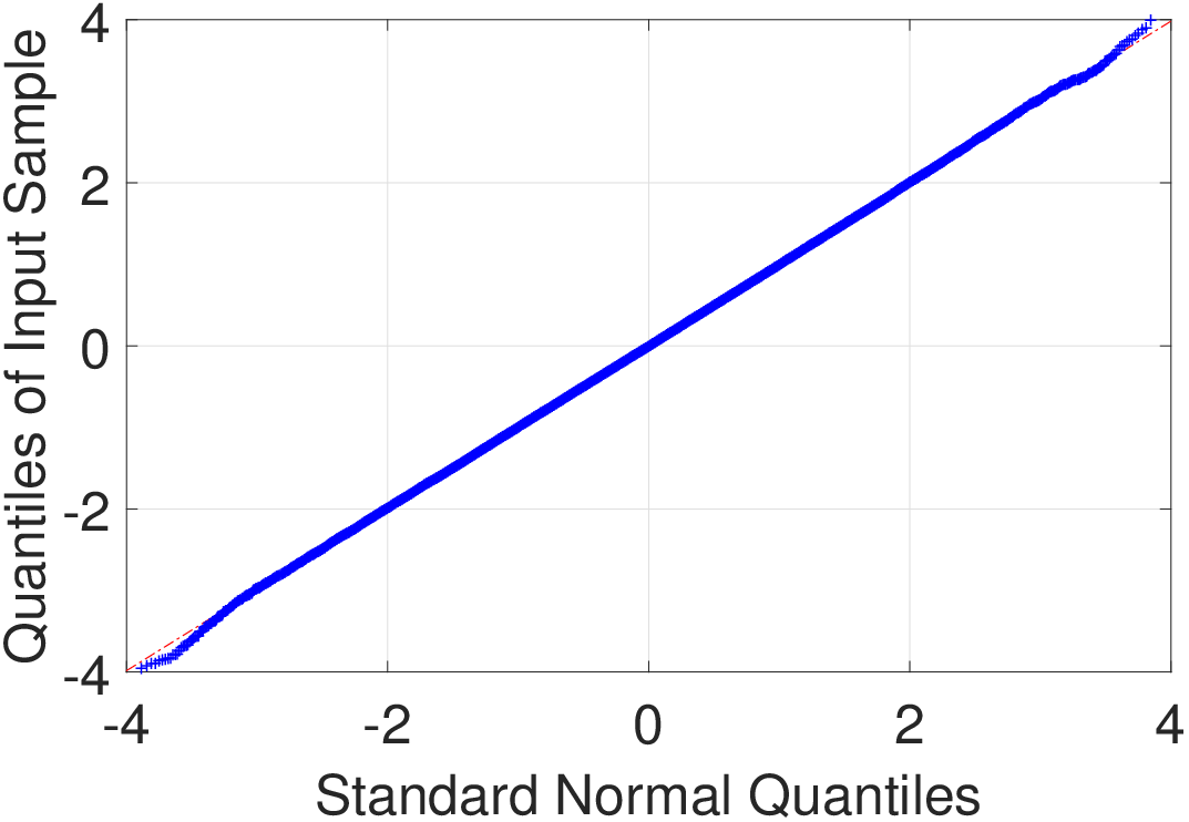
The noise $\varepsilon(t,f)$ can be assumed to follow a normal distribution. To prove this, we collect a set of one-hour CSI data in a static indoor environment with the channel sampling rate $F_{s}=30\,$Hz. The Q-Q plot of the normalized $G(t,f)$ and standard normal distribution for a given subcarrier is shown in Fig. 3(a), which shows that the distribution of the noise is very close to a normal distribution. To verify the whiteness of the noise, we also study the ACF of $G(t,f)$ that can be defined as [29] $\rho_{G}(\tau,f)=\frac{\gamma_{G}(\tau,f)}{\gamma_{G}(0,f)}$, where $\gamma_{G}(\tau,f)$ denotes the auto-covariance function, i.e., $\gamma_{G}(\tau,f)\triangleq\mathrm{cov}(G(t,f),G(t-\tau,f))$. In practice, sample auto-covariance function $\hat{\gamma}_{G}(\tau,f)$ is used instead. If $\varepsilon(t,f)$ is white noise, the sample ACF $\hat{\rho}_{G}(\tau,f)$, for $\forall\tau\neq 0$, can be approximated by a normal random variable with zero mean and standard deviation $\sigma_{\hat{\rho_{G}}(\tau,f)}=\frac{1}{\sqrt{T}}$. Fig. 3(b) shows the sample ACF of $G(t,f)$ when $2000$ samples on the first subcarrier are used. As we can see from the figure, all the taps of the sample ACF are within the interval of $\pm 2\sigma_{\hat{\rho_{G}}(\tau,f)}$, and thus, it can be assumed that $\varepsilon(t,f)$ is an additive white Gaussian noise, i.e., $\varepsilon(t,f)\sim\mathcal{N}(0,\sigma^{2}(f))$.

In the previous analysis in Section III, we assume that the Tx transmits continuous EM waves, but in practice the transmission time is limited. For example, in IEEE 802.11n WiFi systems operated in $5\,$GHz frequency band with $40\,$MHz bandwidth channels, a standard WiFi symbol is $4\,\mu\mathrm{s}$, composed of a $3.2\,\mu\mathrm{s}$ useful symbol duration and a $0.8\,\mu\mathrm{s}$ guard interval. According to [30], for most office buildings, the delay spread is within the range of $40$ to $70\,$ns, which is much smaller than the duration of a standard WiFi symbol. Therefore, we can assume continuous waves are transmitted in WiFi systems.

Based on the above assumptions and (2), (8) can be approximated as

where $\hat{x}$, $\hat{y}$ and $\hat{z}$ are unit vectors orthogonal to each other as shown in Fig. 2, $\mathrm{Re}\{\cdot\}$ denotes the operation of taking the real part of a complex number, and $E_{iu}$ denotes the component of $\vec{E}_{i}$ in the $u$-axis direction, for $\forall u\in\{x,y,z\}$. Then, the auto-covariance function of $G(t,f)$ can be derived as

where Assumptions 1-3 and (3) are applied to simplify the expression and the detailed derivations can be found in Appendix VIII-A.

According to the relation between the auto-covariance and autocorrelation, $\gamma_{G}(\tau,f)$ can be rewritten in the forms of ACFs of each scatterer as

where the right-hand side is obtained by using the relation $E^{2}_{iu}(f)=\frac{E^{2}_{i}(f)}{3}$, $\forall u\in\{x,y,z\}$, $\forall i\in\Omega_{d}$ [24]. The corresponding ACF $\rho_{G}(\tau,f)$ of $G(t,f)$ is thus obtained by $\rho_{G}(\tau,f)=\frac{\gamma_{G}(\tau,f)}{\gamma_{G}(0,f)}$, where $\gamma_{G}(\tau,0)$ can be obtained by plugging $\rho_{E_{iu}}(0,f)=1$ into (11). When the moving directions of all the dynamic scatterers are approximately the same, then we can choose $z$-axis aligned with the common moving direction. Then, the closed forms of $\rho_{E_{iu}}(\tau,f)$, $\forall u\in\{x,y,z\}$, are derived under Assumptions 1-2 [24], i.e., for $\forall i\in\Omega_{d}$,

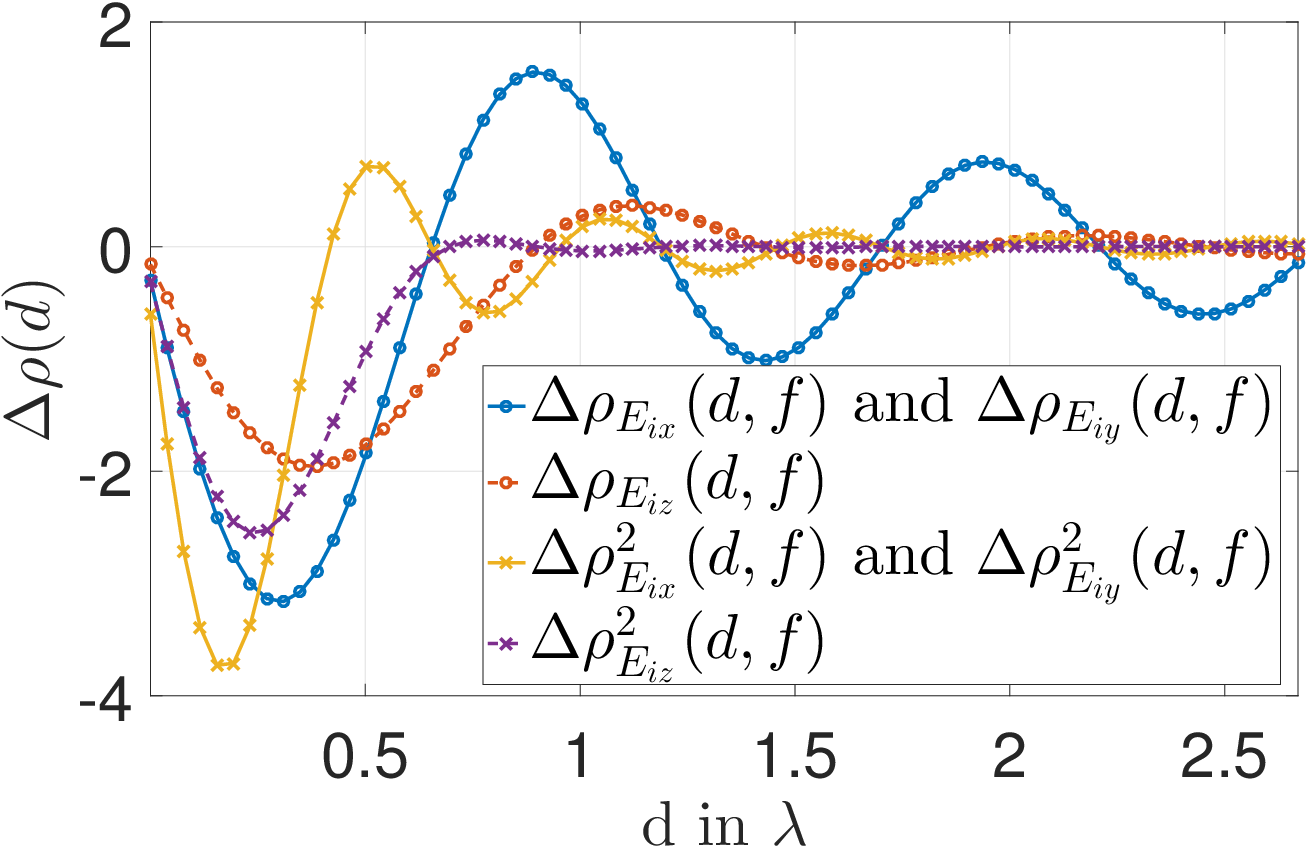
The theoretical spatial ACFs are shown in Fig. 4(a) where $d\triangleq v_{i}\tau$. As we can see from Fig. 4(a), the magnitudes of all the ACFs decay with oscillations as the distance $d$ increases.

For a WiFi system with a bandwidth of $40\,$MHz and a carrier frequency of $5.805\,$GHz, the difference in the wavenumber $k$ of each subcarrier can be neglected, e.g., $k_{\mathrm{max}}=122.00$ and $k_{\mathrm{min}}=121.16$. Then, we can assume $\rho(\tau,f)\approx\rho(\tau)$, $\forall f$. Thus, we can improve the sample ACF by averaging across all subcarriers, i.e., $\hat{\rho}_{G}(\tau)\triangleq\frac{1}{F}\sum_{f\in\mathcal{F}}\hat{\rho}_{G}(\tau,f)$, where $\mathcal{F}$ denotes the set of all the available subcarriers and $F$ is the total number of subcarriers. When all the dynamic scatterers have the same speed, i.e., $v_{i}=v$ for $\forall i\in\Omega_{d}$, which is the case for monitoring the motion for a single human subject, by defining the substitutions $E^{2}_{su}\triangleq\frac{2}{F}\sum_{f\in\mathcal{F}}|E_{su}(f)|^{2}$, $E^{2}_{d}\triangleq\frac{1}{3F}\sum_{i\in\Omega_{d}}\sum_{f\in\mathcal{F}}E^{2}_{i}(f)$, $\hat{\rho}_{G}(\tau)$ can be further approximated as (for $\tau\neq 0$)

where $C$ is a scaling factor and the variance of each subcarrier is assumed to be close to each other.

From (14), we observe that $\rho_{G}(\tau)$ is a weighted combination of $\rho_{E_{iu}}(\tau)$ and $\rho^{2}_{E_{iu}}(\tau)$, $\forall u\in\{x,y,z\}$. The left-hand side of (14) can be estimated from CSI and the speed is embedded in each term on the right-hand side. If we can separate one term from the others on the right-hand side of (14), then the speed can be estimated.

Taking the differential of all the theoretical spatial ACFs as shown in Fig. 4(b) where we use the notation $\Delta\rho(\tau)$ to denote $\frac{\mathrm{d}\rho(\tau)}{\mathrm{d}\tau}$, we find that although the ACFs of different components of the received EM waves are superimposed, the first local peak of $\Delta\rho^{2}_{E_{iu}}(\tau)$, $\forall u\in\{x,y\}$, happens to be the first local peak of $\Delta\rho_{G}(\tau)$ as well. Therefore, the component $\rho^{2}_{E_{iu}}(\tau)$ can be recognized from $\rho_{G}(\tau)$, and the speed information can thus be obtained by localizing the first local peak of $\Delta\hat{\rho}_{G}(\tau)$, which is the most important feature that WiSpeed extracts from the noisy CSI measurements.

To verify (14), we build a prototype of WiSpeed with commercial WiFi devices. The configurations of the prototype are summarized as follows: both WiFi devices operate on WLAN channel $161$ with a center frequency of $f_{c}=5.805\,$GHz, and the bandwidth is $40\,$MHz; the Tx is equipped with a commercial WiFi chip and two omnidirectional antennas, while the Rx is equipped with three omnidirectional antennas and uses Intel Ultimate N WiFi Link 5300 with modified firmware and driver [8]. The Tx sends sounding frames with a channel sampling rate $F_{s}$ of $1500\,$Hz, and CSI is obtained at the Rx. The transmission power is configured as $20\,$dBm.

All experiments in this paper are conducted in a typical indoor office environment as shown in Fig. 5. In each experiment, the LOS path between the Tx and the Rx is blocked by at least one wall, resulting in a severe NLOS condition. More specifically, we investigate two cases:

1. 1.

   The Tx is in motion and the Rx remains static: The Tx is attached to a cart and the Rx is placed at Location Rx #$1$ as shown in Fig. 5. The cart is pushed forward at an almost constant speed along Route #$1$ marked in Fig. 5 from $t=3.7\,$s to $t=14.3\,$s.

2. 2.

   Both the Tx and the Rx remain static and a person passes by: the Tx and Rx are placed at Location Tx #$1$ and Rx #$1$ respectively. A person walks along Route #$1$ at a speed similar to Case (1) from $t=4.9\,$s to $t=16.2\,$s.

Since the theoretical approximations are only valid under the short duration assumption, we set the maximum time lag $\tau$ as $0.2\,$s. In both cases, we compute the sample ACF $\hat{\rho}_{G}(\tau)$ every $0.05\,$s.

Fig. 6 demonstrates the sample ACFs for the two cases. In particular, Fig. 6(a) visualizes the sample ACF corresponding to a snapshot of Fig. 6(e) for different subcarriers given a fixed time $t$ with the time lag $\tau\in[0,0.2s]$, and Fig. 6(c) shows the average ACF $\hat{\rho}_{G}(\tau)$, which is much less noisy compared with individual $\hat{\rho}_{G}(\tau,f)$. In this case, the Tx can be regarded as a moving scatterer with a dominant radiation power compared with the other scatterers, giving rise to the dominance of $E^{2}_{d}\rho^{2}_{E_{iu}}(\tau)$, $u\in\{x,y,z\}$ over the other components in (14). Additionally, $\rho^{2}_{E_{iz}}(\tau)$ decays much faster than $\rho^{2}_{E_{ix}}(\tau)$ and $\rho^{2}_{E_{iy}}(\tau)$, and $\rho^{2}_{E_{ix}}(\tau)=\rho^{2}_{E_{iy}}(\tau)$. Thus, a similar pattern between $\hat{\rho}_{G}(\tau)$ and $\rho^{2}_{E_{ix}}(\tau)$ ($\rho^{2}_{E_{iy}}(\tau)$) can be observed with a common and dominant component $\frac{\sin^{2}(kv\tau)}{(kv\tau)^{2}}$, where $v$ is the speed of the cart and the person. The experimental result illustrated in Fig. 6(c) matches well with the theoretical analysis.

Similarly, for Case (2), Fig. 6(b) shows the sample ACF $\hat{\rho}_{G}(\tau,f)$ for different subcarriers and Fig. 6(d) shows the average sample ACF $\hat{\rho}_{G}(\tau)$, which is a snapshot of Fig. 6(f) given a fixed time $t$ with the time lag $\tau=[0,0.2s]$. Clearly, the pattern of the component $\rho^{2}_{E_{iu}}(\tau)$, $u\in\{x,y\}$, in the sample ACF is much less pronounced than Case (1) shown in Fig. 6(c) and Fig. 6(e). This can be justified by the fact that the radiation power $E^{2}_{d}$ is much smaller than that in Case (1), as the set of dynamic scatterers only consists of different parts of a human body in mobility. Consequently, the shape of $\hat{\rho}_{G}(\tau)$ resembles more closely to $\rho_{E_{iu}}(\tau)$, $\forall u\in\{x,y,z\}$ with a dominant component $\frac{\sin(kv\tau)}{kv\tau}$. Moreover, from Fig. 6(d), we can observe a superposition of $\frac{\sin(kv\tau)}{kv\tau}$ and $\frac{\sin^{2}(kv\tau)}{(kv\tau)^{2}}$ and the weight of $\frac{\sin(kv\tau)}{kv\tau}$ is larger than that of $\frac{\sin^{2}(kv\tau)}{(kv\tau)^{2}}$. We also observe that the embedded component $\frac{\sin^{2}(kv\tau)}{(kv\tau)^{2}}$ has a similar pattern compared with Case (1) since the moving speeds in the two experiments are similar to each other.

Based on the theoretical results derived in Section IV, we propose WiSpeed, which integrates three modules: moving speed estimator, acceleration estimator, and gait cycle estimator. The moving speed estimator is the core module of WiSpeed, while the other two extract useful features from the moving speed estimator to detect falling down and to estimate the gait cycle of a walking person.

In this section, we first introduce the indoor environment and system setups of the experiments. Then, the performance of WiSpeed is evaluated in two applications: human walking monitoring and human fall detection.

In this section, we discuss the system parameter selections for different applications and their impact on the computational complexity of WiSpeed.

In this work, we propose WiSpeed, a universal indoor speed estimation system for human motions leveraging commercial WiFi, which can estimate the speed of a moving object under either device-free or device-based condition. WiSpeed is built upon the statistical theory of EM waves which quantifies the impact of human motions on EM waves for indoor environments. We conduct extensive experiments in a typical indoor environment which demonstrates that WiSpeed can achieve a MAPE of $4.85\%$ for device-free human walking speed monitoring and a MAPE of $4.62\%$ for device-based speed estimation. Meanwhile, it achieves an average detection rate of $95\%$ with no false alarms for human fall detection. Due to its large coverage, robustness, low cost, and low computational complexity, WiSpeed is a very promising candidate for indoor passive human activity monitoring systems.

References

- [1] M. Khan, B. N. Silva, and K. Han, “Internet of things based energy aware smart home control system,” IEEE Access, vol. 4, pp. 7556–7566, 2016.
- [2] S. Pinto, J. Cabral, and T. Gomes, “We-care: An IoT-based health care system for elderly people,” in IEEE International Conference on Industrial Technology (ICIT), pp. 1378–1383, March 2017.
- [3] S. E. Schaefer, C. C. Ching, H. Breen, and J. B. German, “Wearing, thinking, and moving: testing the feasibility of fitness tracking with urban youth,” American Journal of Health Education, vol. 47, no. 1, pp. 8–16, 2016.
- [4] L. Wang, G. Zhao, L. Cheng, and M. Pietikäinen, Machine learning for vision-based motion analysis: Theory and techniques. Springer, 2010.
- [5] S. Z. Gurbuz, C. Clemente, A. Balleri, and J. J. Soraghan, “Micro-Doppler-based in-home aided and unaided walking recognition with multiple radar and sonar systems,” IET Radar, Sonar Navigation, vol. 11, no. 1, pp. 107–115, 2017.
- [6] C.-Y. Hsu, Y. Liu, Z. Kabelac, R. Hristov, D. Katabi, and C. Liu, “Extracting gait velocity and stride length from surrounding radio signals,” in Proc. of CHI Conference on Human Factors in Computing Systems, pp. 2116–2126, ACM, 2017.
- [7] K. Qian, C. Wu, Z. Yang, Y. Liu, and K. Jamieson, “Widar: Decimeter-level passive tracking via velocity monitoring with commodity wi-fi,” in Proc. of the 18th ACM International Symposium on Mobile Ad Hoc Networking and Computing, p. 6, ACM, 2017.
- [8] D. Halperin, W. Hu, A. Sheth, and D. Wetherall, “Tool release: Gathering 802.11n traces with channel state information,” SIGCOMM Comput. Commun. Rev., vol. 41, pp. 53–53, Jan. 2011.
- [9] H. Abdelnasser, M. Youssef, and K. A. Harras, “WiGest: A ubiquitous WiFi-based gesture recognition system,” in Proc. of IEEE INFOCOM, pp. 1472–1480, April 2015.
- [10] K. Qian, C. Wu, Z. Zhou, Y. Zheng, Z. Yang, and Y. Liu, “Inferring motion direction using commodity wi-fi for interactive exergames,” in Proc. of CHI Conference on Human Factors in Computing Systems, pp. 1961–1972, ACM, 2017.
- [11] K. Ali, A. X. Liu, W. Wang, and M. Shahzad, “Keystroke recognition using WiFi signals,” in Proc. of the 21st Annual International Conference on Mobile Computing & Networking, pp. 90–102, ACM, 2015.
- [12] Q. Pu, S. Gupta, S. Gollakota, and S. Patel, “Whole-home gesture recognition using wireless signals,” in Proc. of the 19th Annual International Conference on Mobile Computing & Networking, pp. 27–38, ACM, 2013.
- [13] G. Wang, Y. Zou, Z. Zhou, K. Wu, and L. M. Ni, “We can hear you with Wi-Fi!,” IEEE Transactions on Mobile Computing, vol. 15, pp. 2907–2920, Nov 2016.
- [14] Y. Wang, J. Liu, Y. Chen, M. Gruteser, J. Yang, and H. Liu, “E-eyes: Device-free location-oriented activity identification using fine-grained wifi signatures,” in Proc. of the 20th Annual International Conference on Mobile Computing & Networking, pp. 617–628, ACM, 2014.
- [15] W. Wang, A. X. Liu, M. Shahzad, K. Ling, and S. Lu, “Understanding and modeling of WiFi signal based human activity recognition,” in Proc. of the 21st Annual International Conference on Mobile Computing & Networking, pp. 65–76, ACM, 2015.
- [16] Y. Wang, K. Wu, and L. M. Ni, “WiFall: Device-free fall detection by wireless networks,” IEEE Transactions on Mobile Computing, vol. 16, pp. 581–594, Feb 2017.
- [17] L. Sun, S. Sen, D. Koutsonikolas, and K.-H. Kim, “WiDraw: Enabling hands-free drawing in the air on commodity WiFi devices,” in Proc. of the 21st Annual International Conference on Mobile Computing & Networking, pp. 77–89, ACM, 2015.
- [18] F. Adib and D. Katabi, “See through walls with WiFi!,” SIGCOMM Comput. Commun. Rev., vol. 43, pp. 75–86, Aug. 2013.
- [19] M. Seifeldin, A. Saeed, A. E. Kosba, A. El-Keyi, and M. Youssef, “Nuzzer: A large-scale device-free passive localization system for wireless environments,” IEEE Transactions on Mobile Computing, vol. 12, pp. 1321–1334, July 2013.
- [20] C. Chen, Y. Han, Y. Chen, H. Q. Lai, F. Zhang, B. Wang, and K. J. R. Liu, “TR-BREATH: Time-reversal breathing rate estimation and detection,” IEEE Transactions on Biomedical Engineering, vol. PP, no. 99, pp. 1–14, 2017.
- [21] Q. Xu, Y. Chen, B. Wang, and K. J. R. Liu, “TRIEDS: Wireless events detection through the wall,” IEEE Internet of Things Journal, vol. 4, pp. 723–735, June 2017.
- [22] F. Adib, Z. Kabelac, D. Katabi, and R. C. Miller, “3D tracking via body radio reflections,” in 11th USENIX Symposium on Networked Systems Design and Implementation, pp. 317–329, USENIX Association, 2014.
- [23] P. Murphy, A. Sabharwal, and B. Aazhang, “Design of warp: A flexible wireless open-access research platform,” in Proc. EUSIPCO, pp. 53–54, 2006.
- [24] D. A. Hill, Electromagnetic fields in cavities: deterministic and statistical theories, vol. 35. John Wiley & Sons, 2009.
- [25] D. Tse and P. Viswanath, Fundamentals of wireless communication. Cambridge university press, 2005.
- [26] C. Chen, Y. Chen, Y. Han, H. Q. Lai, F. Zhang, and K. J. R. Liu, “Achieving centimeter-accuracy indoor localization on WiFi platforms: A multi-antenna approach,” IEEE Internet of Things Journal, vol. 4, pp. 122–134, Feb 2017.
- [27] F. Zhang, C. Chen, B. Wang, H. Q. Lai, and K. J. R. Liu, “A time-reversal spatial hardening effect for indoor speed estimation,” in Proc. of IEEE ICASSP, pp. 5955–5959, March 2017.
- [28] T.-D. Chiueh, P.-Y. Tsai, and I.-W. Lai, Baseband receiver design for wireless MIMO-OFDM communications. John Wiley & Sons, 2012.
- [29] R. H. Shumway and D. S. Stoffer, “Time series analysis and its applications with r examples,” Time series analysis and its applications with R examples, 2006.
- [30] R. Van Nee, “Delay spread requirements for wireless networks in the 2.4 GHz and 5 GHzi bands,” IEEE, vol. 802, pp. 802–22, 1997.
- [31] W. S. Cleveland, “Robust locally weighted regression and smoothing scatterplots,” Journal of the American statistical association, vol. 74, no. 368, pp. 829–836, 1979.
- [32] H. Scheffe, The analysis of variance, vol. 72. John Wiley & Sons, 1999.
- [33] S.-J. Kim, K. Koh, S. Boyd, and D. Gorinevsky, “l1 trend filtering,” SIAM review, vol. 51, no. 2, pp. 339–360, 2009.
- [34] Y. Kozlov and T. Weinkauf, “Persistence1D: Extracting and filtering minima and maxima of 1d functions,” http://people.mpi-inf.mpg.de/weinkauf/notes/persistence1d.html, pp. 11–01, 2015.
- [35] F. Bagalà, C. Becker, A. Cappello, L. Chiari, K. Aminian, J. M. Hausdorff, W. Zijlstra, and J. Klenk, “Evaluation of accelerometer-based fall detection algorithms on real-world falls,” PloS one, vol. 7, no. 5, p. e37062, 2012.
- [36] A. Papoulis and U. Pillai, Probability, random variables, and stochastic processes. McGraw-Hill, 2002.