Inference of Dynamic Regimes
in the Microbiome
Abstract
Many studies have been performed to characterize the dynamics and stability of the microbiome across a range of environmental contexts (Costello et al., 2012; Stein et al., 2013; Faust et al., 2015). For example, it is often of interest to identify time intervals within which certain subsets of taxa have an interesting pattern of behavior. Viewed abstractly, these problems often have a flavor not just of time series modeling but also of regime detection, a problem with a rich history across a variety of applications, including speech recognition (Fox et al., 2011), finance (Lee, 2009), EEG analysis (Camilleri et al., 2014), and geophysics (Weatherley and Mora, 2002). However, in spite of the parallels, regime detection methods are rarely used in microbiome data analysis, most likely due to the fact that references for these methods are scattered across several literatures, descriptions are inaccessible outside limited research communities, and implementations are difficult to come across. Finally, the correspondence between regime detection for these applications and for the microbiome is not always obvious.
We distill the core ideas of different regime detection methods, provide example applications, and share reproducible code, making these techniques more accessible to microbiome researchers. Specifically, we reanalyze the data of Dethlefsen and Relman (2011), a study of the effects of antibiotics on the microbiome, using Classification and Regression Trees (CART) (Breiman et al., 1984), Hidden Markov Models (HMMs) (Rabiner and Juang, 1986), Bayesian nonparametric HMMs (Teh and Jordan, 2010; Fox et al., 2008), mixtures of Gaussian Processes (GPs) (Rasmussen and Ghahramani, 2002), switching dynamical systems (Linderman et al., 2016), and multiple changepoint detection (Fan and Mackey, 2015). Along the way, we summarize each method, their relevance to the microbiome, and the tradeoffs associated with using them. Ultimately, our goal is to describe types of temporal or regime switching structure that can be incorporated into studies of microbiome dynamics.
1 Introduction
Microbiome data describe the abundances of bacterial species across multiple samples. In previous chapters, we have studied latent structure across species and samples separately. For example, we have developed interactive visualization techniques to compare subsets of species, and we have applied mixed-membership models to characterize variation in samples. In contrast, our goal here is to study latent structure across species and samples simultaneously. This difference is analogous to the change in perspective obtained by studying a coclustering rather than two separate clusterings, or an ordination biplot instead of simply the scores or loadings. We will focus on the case where samples are collected over time, so that this problem can be understood as one of detecting dynamic regimes, as explained in Section 2
The primary contributions of this chapter are,
- •
The relation of the regime detection problem to several statistical frameworks, and a comparison of the types of interpretation facilitated by each.
- •
The development of experiments to evaluate the practical utility of these different formulations.
- •
A catalog of algorithm pseudocode and complete implementations, to serve as a reference for researchers interested in regime detection.
- •
The design of and code for static visualizations that can be used to evaluate the results of various methods.
In Section 2, we describe the scientific problem of interest in more detail and provide a high-level statistical formulation. In Section 3, we describe approaches which are easy to implement, but that fail to incorporate temporal structure – these serve as reference points for evaluating more complex models. Sections 4 and 5 review and apply smoothing and mixture modeling techniques to this problem.
2 Problem description
In latent variable modeling, our ultimate goal is a succinct representation of complex data. In a way, we can think of the reduced representations as a type of data compression for human interpretation, and as in any (lossy) compression, there is a choice of what structure to preserve. Different reduced representations facilitate different comparisons – for example, clustering bacteria allows easy comparison of taxonomic categories, while clustering samples allows a comparison of full community states.
In the regime detection problem, the comparisons we would like to support are
- •
For each species, should different time intervals be assigned to different dynamic regimes?
- •
Should we distinguish subsets of species as having similar patterns of behavior, with respect to these regimes?
Conceretely, we may expect that over the time course of a study, individual species may switch between stable or unstable, increasing or decreasing, and present or absent regimes, either due to natural ecological dynamics or experimentally induced perturbations. We would like to detect these alternative regimes automatically.
Further, as we often work with hundreds or thousands of bacterial species at a time, we would like to group or relate species according to these regimes, so that (1) we do not need to inspect regime switching behavior for individual species one by one and (2) we can achieve gains in power by pooling across species. The resulting subsets of species can be related to available taxonomic information to draw scientific conclusions about the behavior of different taxa during different sampling periods. For example, for the data of Dethlefsen and Relman (2011), we might be interested in conclusions like “% of species exhibited stability during the first half of the antibiotic time course, while the rest showed decreasing abundances.”
We can frame this analysis problem using the language of latent variables. Let be the sampling timepoints, and index species by . Our goal is to infer a function mapping time by species pairs to an associated latent state, which can be discrete, continuous, or a mixed membership.
We expect the function to be reasonably well-behaved over time. Further, by comparing across different species , we can group or sort species according to their regime membership behavior.
3 Methods baseline
3.1 Hierarchical clustering
As a baseline, Figure 1 provides a heatmap where species are ordered according to a hierarchical clustering tree. Note that clustering trees are invariant under left-right swaps of node children; to fix a unique tree, we order branches so that the average abundance of the left subtree is larger. The resulting ordered heatmap could potentially resolve partitions in the species by time space. A limitation of this approach is that it does not provide any clustering for the timepoints, even if blocks across timepoints seem to appear in the resulting heatmap. Coclustering species and timepoints is not a sufficient alternative, because the blocking across timepoints must respect the known temporal order. On the other hand, advantages of this approach are that it is simple to implement and interpret.
The figure generated by hierarchical clustering is sensitive to several choices,
- •
Transformations: Different transformations might be more effective representations of the underlying data.
- •
Distance: Different distances accentuate different types of variation.
For example, some natural transformations are
- •
: Raw count data in microbiome data sets tend to be heavy tailed, but with a large spike at 0. An transformation behaves like a -transformation for large counts, but goes through the origin – this downweights coordinates with large counts. This can be seen from the representation .
- •
Innovations: Rather than clustering the raw series, we can cluster the first differenced series. This will cluster series that have similar changes between neighboring timepoints, even when their overall values are quite different. This can highlight bacterial series with similar dynamics, at the cost of ignoring differences in overall abundances.
- •
Binarized: We can transform the series into . This loses substantial information, but measuring differences in presence-absence patterns in microbiome studies can be scientifically meaningful.
On these transformed data, we now need to compute pairwise distances between series. Three choices that we consider are,
- •
Euclidean: This distance is ideal when clusters have a spherical shape.
- •
Jaccard: This is a distance between pairs of length binary sequences and defined as
or one minus the fraction of coordinates that are both 1. The motivation for this distance is that coordinates that are both 0 should not contribute to similarity between sequences, especially series that are dominated by 0s. We apply this distance to the binarized version of the species counts.
- •
Mixture: Since any convex combination of distances is still a distance, we can define mixtures of distances that reflect several characteristics of the data.
In general, we have no quantitative approach for comparing the clusterings obtained by different distances. Instead, we compare the resulting heatmaps, noting how different patterns are identified by different approaches.
3.1.1 Example
Now we use hierarchical clustering the data of Dethlefsen and Relman (2011). The heatmaps in Figures 1 through 2 describe which species have similar behaviors according to Euclidean and Jaccard distances, respectively. See Supplementary Figures 20 through 22 for variations on the distance and transformation. The most important takeaways from these figures are that some groups of bacteria are more strongly affected by the antibiotic treatment, and there is variation in the time it takes to recover.


As expected, different distances group series according to the features that define the distance. For example, the Jaccard distance, used in Figure 2, groups series with similar zero patterns, even if their associated abundances are very different. On the other hand, the Euclidean distance tends to group series with similar averages, and there is less blocking by presence-absence structure. Note that patterns of response to antibiotics form subclusters within taxonomic families. This suggests that while phylogeny certainly relates to patterns of abundance, variation occurs at levels of granularity more subtle than family level.
To summarize behavior within clusters, we display the centroids in Figures 3 4. Evidently, some of the clustering structure is due to the presence of species within only some of the subjects. Further, differential responses can be seen within some of the panels. For example, cluster 17 in Figure 3 includes bacteria that are affected by the first antibiotics time course, but only for subjects D and F, and which are only affected in subject D during the second time course.


The fact that the data include many zeros makes the mean a somewhat misleading cluster summary. Instead, we can decompose the summary into a presence-absence component and a conditional-on-presence component. The presence-absence component computes the proportion of bacteria that are present at any given timepoint, while the conditional-on-presence component computes the time averages among bacteria with strictly positive abundance.
3.2 CART
While placing similar time series near to one another suggests time windows where the series behave similarly to one another, the hierarchical clustering approach presented above does not explicitly partition timepoints into windows with distinct behaviors. In this section, we consider an alternative that provides such a partitioning.
The main idea is that a regression tree that uses to predict provides a partition of the space in which lives, where has lower variation within than between partitions (Breiman et al., 1984). We apply the hierarchical clustering approach from the previous section to obtain an ordering across species. We write the timepoint for the sample as Then, we model the count for the species in the sample as where , the space of decision trees. The output of interest is the fitted partition on .
For completeness, we review the CART algorithm. Following (Friedman, 2017), we can describe it in terms of (1) the structural model, (2) the score criterion for choosing between models, and (3) the search strategy used to produce the final fit.
The structural model is the class of functions that can be expressed as
where is a partition of the covariate space and are constants associated with each partition element.
For regression, the criterion is the expected generalization squared-error between and the associated with the partition element in which lies – we will denote this by . In classification, the corresponding criterion is the expected missclassification error. More precisely, we calculate empirical risks,
for regression and
for classification, where is the loss induced by missclassifying as . Since the empirical risk on the training data underestimates generalization error, these estimates are constructed on test sets.
To obtain a fitted , the algorithm must identify a partition and constants that (approximately) minimize the score criterion. Given a fixed , fitting is straightforwards, since the score decouples across partition elements – in regression the minimizers are averages of the within partition elements, while in classification they are majority votes. On the other hand, finding the optimal is an intractable combinatorial optimization problem, and the search strategy resorts to a greedy approach in hope of a reasonable local minimizer.
More precisely, the final partition is found by recursively splitting the input space and then pruning away splits that seem less relevant. At the first step, the partition consists of a single , equal to the entire covariate space, and it is split on covariate at position , chosen to solve the optimization
where and (for “left” and “right”) are a splitting of along feature feature at position .
This procedure is iterated recursively. That is, at the iteration, the next split solves nearly the same optimization,
where the main difference is that we must now choose which of the previously defined partition elements to split.
This is done for some prespecified number of splits, . This partition is often unecessarily highly resolved, and it can improve generalization performance to introduce a pruning step. Let denote the “cost” of a (potentially intermediate) partition element , defined by
where . can be interpreted as the amount of improvement to the score criterion that the split must provide in order to be accepted, and it is fixed in advance. The final partitioning is obtained by choosing to split or merge each intermediate partition element so that is minimized. Specifically, if , then all descendant nodes (subpartition elements) are merged into . Otherwise, the left and right splits are accepted. These choices are made sequentially, from the bottom up.
3.2.1 Example
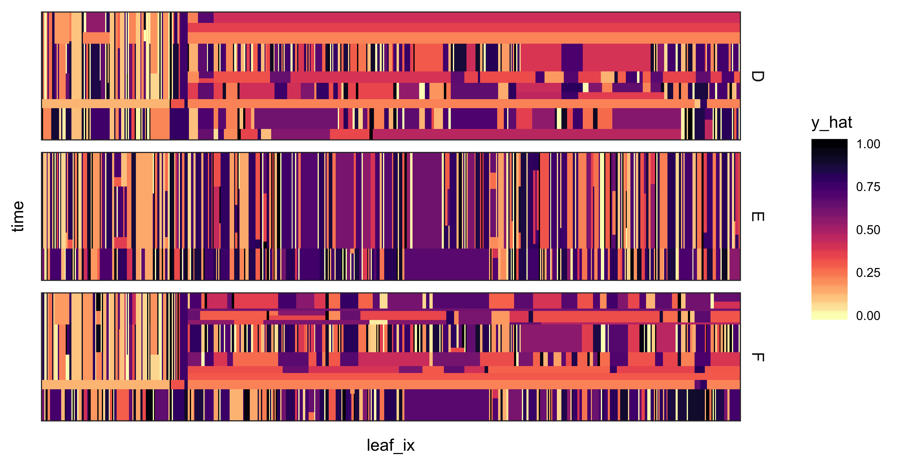
Example output from this approach is provided in Figure 5. Note the presence of two light vertical stripes in subjects D and F – these correspond to the two antibiotic treatment regimes. In general, “tall” blocks are more common than “wide” ones. This reflects the fact that timepoints within bacteria tend to have more similar abundances, compared to multiple bacteria at a single timepoint, even when those bacteria have been ordered by a hierarchical clustering.
One interesting detail is the delayed, or sometimes nonexistent, recovery after the first antibiotic time course among a cluster of bacteria near the bottom-left of the panel for subject F. This long-term impact of antibiotics on bacterial populations, at least in one subject, was a central finding in Dethlefsen and Relman (2011). Observe that a similar pattern is visible after the second antibiotic time course among subject D, also for species near the bottom-left of the panel.
Related views are given in Supplemental Figures 23 through 26. Supplemental Figures 25 and 26 decompose the CART prediction problem into a binary part and a conditional-on-present component, using the hurdle heuristic.
Two limitations become clear in this example application. First, partitioning across species seems hard to obtain simultaneously across all subjects – in Figure 5, there seem to be no “wide” blocks for Subject E. This is a consequence of first ordering all species according to a hierarchical clustering based on all subjects. A potential solution would be to cluster the species separately across subjects, trading off the ability to match the same species across several panels in order to better study species blocking within subjects.
Second, these global views of the data make it difficult to inspect individual species and sample identities. Potential solutions are (1) link necessary supplemental (e.g., taxonomic) information within the static view, through a shaded taxonomic-family stripe, as in Figure 1 (2) construct an interactive version of these plots, where hovering over a partition element provides focused information about that element (e.g., the species identities it contains), in the spirit of our centroidview package11 1 https://github.com/krisrs1128/centroidview.

4 Smooth temporal models
In Section 3, we described distance and regression-based techniques to approaching the questions outlined in Section 2 of identifying which subsets of species have similar abundance profiles during which windows of time. In particular, we have avoided direct modeling of abundances across species or over time. In this section, we adopt this alternative direct modeling approach, using the distance and regression-based methods of Section 3 as a reference for what analysis is possible with minimal effort.
We first review two fundamental approaches to probabilistic temporal modeling which are used as building blocks for the more advanced methods in Section 5: Linear Dynamical Systems in Section 4.2) and we consider Gaussian Processes in Section 4.1). These approaches are designed for single time series, or collections of independent ones. However, models that consider collections of related time series can be constructed from these, by introducing latent variables.
4.1 Gaussian Processes
Gaussian Processes (GPs) provide a prior over classes of stationary, smoothly varying functions. Their appeal as a building block for probabilistic models lies in the fact that they are nonparametric – they can adapt to more complex functions as more data arrives – while still admitting tractable inference. One of the simplest GPs models observations as
where , meaning that for any collections of covariates , we have
and are called the mean and covariance functions, respectively. We will denote the covariance matrix of applied to pairs of by . A plate diagram representing this model is provided in Figure 6.
It is common to initially center the data before analysis, in which case we can assume . Further, any positive-definite covariance function can be used – a common choice is the Gaussian covariance,
where can be , which assumes similar degrees of smoothness across all coordinates, , which allows different smoothness along different axes, or , which allows variation along directions that are not axis-aligned. While the Gaussian covariance provides a reasonable default, it is good practice to adapt the covariance function to the data problem at hand, accounting for seasonality, multiple scales of variation, or the presence of outliers, see Section 5.4.3 of (Rasmussen and Williams, 2006) for an in depth example. Note that the covariance function is responsible for the GPs poor ability to model transient events, compared to smooth trajectories. However, multiscale behavior can be modeled by introducing mixtures, as we will see in Section 5.
In this model, the posterior of is available analytically, by virtue of Gaussian-Gaussian conjugacy. Consider evaluating the function at new points , denoted by . The joint of and is
which yields the posterior,
where
Note the matrix inversion in the covariance calculation. This is the source of the complexity of using standard GPs, though a variety of fast approximations have been proposed, exploiting the sparse, banded, or block structure often present in covariance matrices (Quinonero-Candela et al., 2007).
In this computation, we have assumed the the kernel hyperparameters are known22 2 For example, in the Gaussian covariance case, this has the form . In reality, these must be inferred from the data. Two standard approaches are based on maximizing (1) the marginal likelihood of and (2) the cross-validated predictive likelihood. The first approach leverages the fact that the marginal likelihood,
and its gradients over have a closed form, and so can be optimized.
The cross-validation approach instead maximizes the average predicted log probability,
which can also be found analytically, by conditioning the marginal for .
4.2 Linear Dynamical Systems
Linear Dynamical System models (LDSs) treat an observed time series as a transformation of temporally evolving latent states. There have been many proposals that allow general transformation and state evolution behavior (Hostetler and Andreas, 1983; Wan and Van Der Merwe, 2000), but a fundamental starting point is the Linear-Gaussian dynamical system,
The ’s are a Markov chain of latent states, while the ’s represent the observed emissions from it. and govern the dynamics of the underlying process, while and describe the emission structure. The associated graphical model is provided in Figure 7.
There are two conceptual components to fitting this model,
- •
Inference: Even if were known, there is often value in estimating the latent .
- •
Learning: Typically, the parameters are unknown, and must themselves be learned from the data.
Further, inference can be approached in several different ways, depending on problem context and constraints. Among the most common approaches are
- •
Filtering: Update beliefs of the current latent state in an online fashion. Quantitatively, the goal is to estimate the distribution .
- •
Smoothing: Use the full history to estimate beliefs of latent states at each time. This means to compute for each .
- •
Forecasting: Predict the next few latent states given all observations so far. For example, we might be interested in .
We first describe inference in detail, before explaining how inference and learning can be alternated to fit models on real data. Due to the Linear-Gaussian assumption, the conditionals required by filtering and smoothing are still Gaussian; however, their means and covariances are not immediately apparent. It turns out that, for both filtering and smoothing, they can be efficiently computed via dynamic programming recursions. In the literature, these are referred to as the Kalman Filtering and Rauch-Tung-Striebel (RTS) smoothing recursions.
Consider the filter, where the goal is calculation of . We will assume . We could alternatively fix it to a constant – the point is that the distribution for must be known.
For , define the one-step-ahead and updated means and covariances by
The means and covariances are the main quantities of interest in filtering. The filtering algorithm is detailed in in Algorithm 1. It can be thought of as a forwards pass through the observed sequence, updating means and covariances along the way.
The derivation is as follows. For the predict step, use the tower property and the law of total variance,
For the update step, use Gaussian conjugacy to obtain the required means and covariances and the matrix inversion lemma to express them more concisely. More precisely,
and both densities on the right are Gaussian – the first is the likelihood of the observed while the second is the predict-step density derived above. By Bayes’ rule, the posterior is Gaussian with increased precision,
| (1) |
and shrunken mean,
| (2) |
Recall the matrix inversion lemma,
and apply it to equation 1 to find
according to the definition of in Algorithm 1.
Substituting this expression, we can simplify equation 2,
where for the simplification on the second half of the second line,
we again used the matrix inversion lemma.
While the Kalman filter makes a forwards pass over the observations to estimate the latent state means and covariances as data are made available, the RTS smoother can be understood as a pair of forwards-backwards sweeps that propogate information from all observations to the latent state estimates obtained by filtering. Define the quantities,
which completely determine the smoothed distributions of interest. The forwards pass in RTS smoothing is identical to the Kalman filter, and pseudocode for the backwards pass is provided in Algorithm 2.
To see why this update works, first consider the joint behavior of neighboring times,
because
Conditioning, we obtain
Since is independent of conditional on , this is enough to compute the full smoothed means and covariances. By the tower property,
and similarly by the law of total covariance,
4.2.1 Zero-inflation in dynamical systems
After transformations, many microbiome data sets can be viewed as a mixture between a continuous, nonnegative component and a spike at 0. Such data has a rich history in statistics, and has been approached using hurdle and tobit modeling ideas (Min and Agresti, 2002). In this section, we take a detour from our review of standard temporal modeling methods, to describe a variation of the standard LDS, called the dynamic tobit model (DTM), that is designed for the zero-spiked density situation.
The basic idea of the DTM is to truncate an LDS below some threshold, so that the continuous positive data correspond to excursions of the LDS above some threshold, while the zeros correspond to parts of the path below the threshold. That is, the observed data are modeled according to
Note that last two equations are exactly those defining an LDS, but that , and are all unobserved data in this setting. As before, are model parameters to be learned.
There are several approaches to inference in this model, including particle filtering (Doucet et al., 2000), Monte Carlo EM (Manrique and Shephard, 1998), and Gibbs sampling (De Jong, 1997; Wei, 1999). In many of these approaches, recursions like those used in the Kalman filter can be used to perform efficient sampling and estimation.
To give an exaple, we review one method here, the scan sampler of De Jong (1997). For simplicity, we will assume that is known and equal to zero. The scan sampler iterates filter and smoother-type calculations for , at each step sampling from a distribution with mean and variance . In the Gaussian case presented above, this provides the exact posterior, though De Jong (1997) describe its utility for general exponential families.
To initialize the scan sampler for the DTM, first set for all , then perform a Kalman filter and smoother step. This gives estimates of the following quantities, using notation analogous to that in the previous section,
The idea of the scan sampler is to iteratively compute and such that
so that sampling can cycle forwards and backwards through coordinates of , drawing . Details of the derivation can be found in (De Jong, 1997), we simply describe the updates necessary to compute and , along with an example application. In an initial backwards pass through the data, we compute
where is the Kalman gain matrix at time and
The remain fixed after this initial scan, and only sampling proceeds only by cycling through the . During the forwards scan, is updated according to
where , while for backwards scans, the analogous updates are
Each time a is computed, it is used to update the unobserved by sampling from .
Code implementing these updates is available at https://github.com/krisrs1128/tsc_microbiome/tree/master/src/scan. We have also provided an example application to a real microbial abundance time series, whose results are provided in Figure 8.

5 Temporal mixture models
In the models considered in Section 4, all time windows exhibit comparable behavior. From the problem description of Section 2 however, we would expect changes in the behavior of the system during different temporal regimes. In this section, we describe probabilistic models that generate this sort of behavior. The unifying probabilistic “trick” that helps accomplish this goal is the introduction of latent variables specying which regime the system is in at any given timepoint.
5.1 Hidden Markov Models
The idea behind Hidden Markov Models (HMMs) is similar to that of LDSs, with the exception that the are no longer thought of as continuous latent variables. Instead, each is assigned one of a few discrete states, which switch between one another according to a Markov chain.
An informal analogy is how I choose to listen to different music tracks. For a few days, I might be mostly listening to sonatas by Beethoven and Schubert, because I’m in a latent state that prefers German piano sonatas. I might be more likely to transition from here to French chamber music than, say, LA punk. So, my underlying style preferences evolve according to a Markov chain , which is in turn reflected by the actual tracks that I listen to.
More formally, we suppose comes from some initial distribution and has some transition probability matrix whose rows lie in , the dimensional simplex. Conditional on , is emitted according to the density , one of emission densities . Concisely,
As in LDSs, fitting this model can be broken into inference and learning steps, which estimate the distributions of the conditional on observed data and which fit the model parameters , respectively. Alternating these two steps optimizes the expected complete data loglikelihood in an EM algorithm.
The -step, which infers latent states, is referred to as the forwards-backwards algorithm. This procedure parallels the Kalman filter (forwards) and smoother (backwards) algorithm for inference in LDSs. First, we find a simple expression for the analog of the filtered densities, based on the Markov property for the ’s,
The first term is known by assumption, while the second can be computed from the previous filtered probabilities,
The forwards pass of the Forwards-Backwards algorithm alternates these two steps (“update” and “predict”), after initializing , as described in Algorithm 4.
The backwards pass computes the analog of the smoothed densities, based on the observation33 3 This is the same observation used in the derivation of the Kalman smoother. that is independent of the future conditional on ,
The second term on the right hand side is available from the forwards pass. The first term is computed during the backwards pass, which initializes and then accumulates the “future observation” densities from right to left,
The backwards pass is summarized in Algorithm 5.
In the M-step, the parameters , and must be learned. Estimation of the per-regime parameters can be done separately for each . For example, if HMM has Gaussian emissions, , then
while, regardless of the emission structure, the Markov chain parameters can be estimated via
5.1.1 Example
In the context of regime detection in the microbiome, we imagine a few underlying states shared across all bacteria, with means ranging from high abundance to complete absence. Within each species, states evolve independently according to a Markov chain. Note that, while we do share across species when estimating underlying parameters , we do not tie together latent indicators across species. Specifically, we use a DAG that factors across all species – given , all species abundances follow independent HMMs.
Therefore, in the -step (the forwards-backwards algorithm) the can be estimated in parallel across all species. The -step is modified so that mixture component parameters and transition probabilities are estimated simultaneously across all species, for example, the new mean update for cluster in an HMM with Gaussian emissions becomes
We employ this approach on the antibiotics data described in Section 3.2.1. The results are summarized in Figure 9 and Supplementary Figure 27, which display the modes and raw probabilities of the smoothed probabilities after applying EM. As in Figure 3 and its counterparts made through hierarchical clustering, rows correspond to individual species, while columns are samples sorted by time. The three main panels are the three subjects in the study. Rows are ordered according to a hierarchical clustering on Euclidean distances between sequences , where . The intensity of the shading of each cell corresponds to the average value for that mode.
We can think of Figure 9 as a smoothed version of the raw heatmaps made through hierarchical clustering. By coarsening the raw values into cluster centers, certain patterns are more easily visible. For example, in addition to effect of the two antibiotics time courses across all subjects, we note that
- •
The effect of the first antibiotic time courses is more prolonged in subject F, and in some cases species disappear for most of the remainder of the experiment. Some of these species seem to have also disappeared from subject D, but most others recovered in both subjects D and E.
- •
The phenomenon in which some species become more abundant during the time courses – presumably filling in newly emptied niches – is stronger in subject E than the others. Further, some species that exhibit this behavior in subject E respond differently within subjects D and F, becoming less abundant rather than more.
Note that, while smoothing makes the antibiotic effect clearer among moderately and highly abundant species, variation among rarer species, to which all timepoints are assigned to the rare abundance state, is obscured. This could be remedied by increasing , at the cost of increasing the complexity of interpretation for abundant species.
Instead of displaying the sequence of modes , Supplemental Figure 27 provides the individual probabilities across . The vertical panels distinguish between different , while transparency represents the size of the probability – smaller probabilities are more transparent. The colors are associated with centroid means, as before. In this application, most probabilities seem near one, so this view adds little to that in Figure 9. However, this does suggest the possibility of overfitting, which we address by introducing priors on in Section 5.1.2.
The estimated transition probabilities between states, ordered in terms of increasing , are displayed below.
      1     2     3     4
1 0.810 0.159 0.028 0.003
2 0.389 0.527 0.083 0.002
3 0.077 0.094 0.810 0.019
4 0.027 0.007 0.056 0.910
Unsurprisingly, most transitions remain in the same state, and any departures are generally restricted to states with similar s. Generally, there appear to be more transitions downwards than upwards, and the sum of transitions into state 1 is higher than the sums for the rest. This can likely be attributed to the antibiotic effect, which reduces abundances of species that recover at differential rates.
As in Figure 3, the primary drawback of this display is the difficulty in linking observed species trajectories to species or taxonomic detail. To easily link the smoothed HMM estimates to raw time series values and species descriptions would require either splitting the view across taxonomies or introducing interactivity.

5.1.2 Sticky HMMs
Sticky HMMs are an extension of ordinary HMMs designed to induce additional “stickiness” in state transitions – states should be encouraged to remain unchanged over longer stretches of time. To practically implement this basic idea, a Bayesian view is useful, and we describe inference in detail. An application to the antibiotics data follows this explanation.
Consider the standard Bayesian HMM, which places priors on the rows of the transition probability matrix and conjugate priors on . The main idea of the sticky HMM is to introduce a “stickiness” parameter to the Dirichlet prior44 4 Here, is the vector with a in the coordinate and zeros everywhere else.: . This means that draws from the prior on will have larger weight along the diagonal, depending on the size of , and since diagonal elements correspond to self-transitions, chains drawn from the prior will be “sticky.”
To draw samples from , we consider a block Gibbs sampler that parallels EM (Frühwirth-Schnatter, 2006). In place of the -step, we draw from the conditional using a variation of the forwards-backwards algorithm, and in place of the -step, we draw from and . We detail this below, following the derivation of (Fox, 2009).
First consider sampling . Since each sequence is independent of all others, given , we can sample the separately across each , so for the explanation below, we drop this subscript. By the DAG structure of the HMM, the probability a single sequence can be decomposed according to
| (3) |
If we could calculate each of these individual probabilities, then one mechanism for sampling the entire sequence would be to first sample , then sample given , etc. Note that the first term has a different structure than the rest (it doesn’t depend on any previous ), so we analyze it first,
where we used the fact that . The first two terms are easy to sample, and we will show below that terms of the form can be calculated efficiently using a backwards-pass type recursion.
Consider now the terms in the product of equation 3. By Bayes rule,
The second term is a likelihood, and the third will be calculated by the backwards-pass. Note that the first term can be further reduced to
since we care only about the terms involving , as we are sampling .
We next describe how to compute the terms efficiently, as promised above. Consider storing these terms in a matrix, whose element is . The bottom row is initialized according to
Then the recursion computes the row from the according to
Next consider sampling from the conditional of transition probabilities between the states. The main observation is that we can use Dirichlet-Multinomial conjugacy jointly across all sequences. That is, defining
we have
and therefore
| (4) |
Since given , is independent of all other parameters and data, this completely specifies this Gibbs sampling step.
To sample , we use assumed conjugacy separately across each class . For example, if and
and if
then the usual Normal-Inverse Gamma posterior can be used, after subsetting to those samples with ,
An implementation of this sampler is available at https://github.com/krisrs1128/tsc_microbiome/blob/master/src/hmm/bayes_hmm.R.
5.1.3 Example
An application of the sticky HMM to antibiotics data is provided in Figure 10. As in Section 5.1.1, we choose and a Gaussian emission model. After manual experimentation, we set . We have reordered species according to a hierarchical clustering on the new estimated means. The interpretation suggested by this figure is generally quite similar to those for the nonsticky HMM. As before, the antibiotic treatments are visible across all subjects, especially D and F, with differential recovery rates among certain species, and some species in subject D that seem to increase in abundance during the first antibiotic time course and one timepoint during the interim. In contrast to the HMM fitted with EM, it is easier to pick out a block of species among the Ruminoccocus that are strongly affected by the first, but not second, antibiotics time courses, especially in subject F. On the other hand, species that increase in subject D during the first time course are now split across a few blocks, when they had been all grouped together in Figure 9. Overall, the clustering seems somewhat more interpretable in the sticky HMM, though we have not quantitatively compared different metrics for two clustering approaches.

As before, we can study the estimated transition matrices between pairs of states. These are printed below, with states sorted from lowest to highest emission means.
       3     4     1     2
3  0.775 0.113 0.044 0.068
4  0.160 0.414 0.170 0.256
1  0.073 0.300 0.196 0.431
2  0.025 0.083 0.083 0.809
Unlike EM, Gibbs sampling can provide a sense of the uncertainty of these parameter estimates. The standard errors of the cells for these transition probabilities are printed below.
       3     4     2     1
3  0.005 0.007 0.002 0.004
4  0.010 0.017 0.011 0.017
1  0.009 0.014 0.031 0.011
2  0.002 0.006 0.006 0.004
Counterintuitively, while the sticky HMM was proposed to model state persistence, the probabilities of self-transitions estimated here are lower than those estimated for the ordinary HMM. One explanation is that the Dirichlet priors placed on the rows of the transition matrix in the sticky HMM serve as regularizers. Decreasing the Dirichlet concentration parameter would likely return us to more extreme self-transition estimates from EM. However, these regularized transition probabilities are perhaps more believable – simply because certain transitions have not been previously observed doesn’t mean they should be given probability 0.
5.1.4 Sticky HDP-HMMs
Next we describe a Bayesian nonparametric variation of sticky HMMs first proposed in (Fox et al., 2008). There are two sources of motivation for such a model,
- •
It is appealing to allow the complexity of the fitted model to increase as more data becomes available. This drove the original HDP-HMM proposal of (Teh, 2006).
- •
State persistence – i.e., stickiness – can yield better fitting and more interpretable HMMs. This turns out to be especially relevant in the nonparametric setting, where there is a danger of overfitting by introducing many short-lived states.
The proposal of (Teh, 2006) replaces the usual sticky-HMM on rows of with an prior55 5 This refers to a Hierarchical Dirichlet Process prior with component concentration , shared concentration , and baes measure , explained in more detail below.. Note that a prior on its own would not be sufficient, since two separate draws from a prior with a continuous base measure would have distinct atoms almost surely. Hence, it would be impossible to align the rows of the transition matrix according to a set of common states. By using a base measure instead, the prior allows sharing of states across .
More formally, an HDP-HMM models a sequence , emitted from a latent Markov chain ,
with a prior on the rows of the transition matrix given by
Since each of the transition matrix rows are centered around the base measure , the rows are i.i.d., and there is no stickiness.
To induce state persistence, first consider a stick breaking representation DP base measure where the sequence is drawn from a distribution66 6 The GEM distribution (Gnedin and Kerov, 2001) can be described by a stick breaking constrution. Specifically, can be constructed by taking , where independently. . Cosider a modified base measure, , which places additional mass on the atom for the latent state. Using as a base measure for encourages the state to return to itself. For completeness, the prior for rows of the transition matrix now has the form,
Fox (2009) describes two inferential approaches for this model: an exact one that extends Chinese Restaurant Franchise analogy developed by (Teh, 2006) and an approximate blocked Gibbs sampler. Here, we describe the blocked Gibbs sampler, since while it is only approximate, it mixes more rapidly77 7 Implementations of both approaches are available at https://github.com/krisrs1128/tsc_microbiome/tree/master/src/hmm. This is because the exact sampler can only swap cluster labels one at a time, which means it must pass through low probability valleys in the posterior where a cluster is awkwardly split in half before reaching a potentially higher mode.
The idea of the blocked Gibbs sampler is to sample all the assignments simultaneously using the same forwards-backwards variant used for inference of the sticky HMM in Section 5.1.2. A difficulty in directly applying this strategy is that we no longer have a finite number of states from which to sample. To get around this issue, Fox et al. (2008) employs Ishwaran and Zarepour (2002)’s “weak-limit” approximation,
where is truncation level chosen large enough so that the number of clusters visible in the observed data modeled by an exact DP would usually be smaller than . Note that there is a tradeoff here between statistical and computational efficiency – larger brings us closer to the exact model but requires more involved computation.
With this approximation in hand, we can now describe a tractable sampler. The full parameter set consists of . To facilitate sampling, three sets of auxiliary variables , and are introduced. Each term is sampled one at a time, from its full conditional.
Some mnemonics can help with tracking notation,
- •
track the number of transitions from states to if there had been no stickiness.
- •
counts the number of times stickiness is invoked in state .
- •
counts the number of transitions from to after accounting for state persistence.
We simply state the conditionals required in each step of the Gibbs sampler. A detailed derivation is provided in (Fox, 2009). The conditional for is
where . The updates for and are the same as those for the (finite) sticky HMM, described in Section 5.1.2. Next consider sampling the auxiliary variables. To sample , draw
where counts the number of observed transitions from states to among the , which we have conditioned upon. The distribution of is sometimes called a Chinese Restaurant Table distribution, because it counts the total number of tables that have been occupied in a CRP after a certain number of customers have arrived (Zhou and Carin, 2012), which is a sum of Bernoulli decisions to join an old table or occupy a new one.
For , the conditional can be shown to be
where . is set deterministically, according to
Cycling these updates provides a blocked Gibbs sampler for the sticky HDP-HMM.
5.1.5 Example
An application of the HDP-HMM to the antibiotics data is summarized in Figure 11. We ran a Normal-Inverse Gamma emissions version of the sampler for 2000 iterations, initializing the model using the model using means and covariances from clusters found with -means. We set , , , and .
As in the original parametric HMM displayed in Figure 9, Figure 11 clearly highlights the antibiotic regimes across subjects D and F, as well as the differential recovery rates among some species in subject F. However, with our choice of , there tend to be many transient states, represented by the increased number of intermediate colors between light yellow and dark purple. We can understand this figure as a kind of smoothing using a low bandwidth. Decreasing and increasing leads to a higher concentration in few states, and a more strongly smoothed representation of the data.

Estimated transition probabilities are printed below. While in theory the transition matrix is infinite dimensional, the weak limit approximation provides clusters plus one additional category containing the rest of the mass from the DP for that row. States are ordered from lowest to highest emission mean.
       9     6     8     5     3     4    10     2     1     7
 9 0.016 0.008 0.007 0.003 0.002 0.002 0.003 0.006 0.004 0.007
 6 0.011 0.014 0.027 0.013 0.006 0.009 0.010 0.002 0.017 0.018
 8 0.012 0.019 0.035 0.029 0.015 0.010 0.017 0.000 0.027 0.034
 5 0.011 0.036 0.023 0.030 0.025 0.011 0.026 0.000 0.023 0.034
 3 0.009 0.037 0.010 0.019 0.027 0.020 0.041 0.000 0.021 0.037
 4 0.007 0.030 0.008 0.008 0.016 0.022 0.057 0.000 0.014 0.040
10 0.001 0.008 0.006 0.016 0.020 0.037 0.284 0.000 0.059 0.176
 2 0.010 0.011 0.007 0.002 0.005 0.022 0.081 0.020 0.035 0.088
 1 0.005 0.021 0.011 0.009 0.011 0.014 0.051 0.000 0.020 0.008
 7 0.002 0.005 0.002 0.002 0.003 0.005 0.014 0.000 0.005 0.004
As in the other HMM-based methods, the sticky HDP-HMM places most mass in the transition matrix along the diagonal, corresponding to self-transitions. As in the sticky HMM, self-transitions are somewhat more regularized than in the HMM estimated through EM. Transitions from the highest to the lowest states are more common than transitions in the opposite directions. This corresponds to the fact that rapid drops after antibiotic time courses are somewhat more common than rapid recoveries.
In addition to summaries of the model results, it is informative to investigate properties of the sampling routine, to diagnose potential defects or limitations. Supplemental Figure 29 displays the evolution of state assignments over iterations. The variation in state colors at the bottom of the figure represents the initial burn-in period. Most states, especially those corresponding to low abundance states, seem relatively fixed across Gibbs sampling iterations. In some situations, this would be a marker of poor mixing of the block sampler, in spite of its performing full forwards and backwards sweeps during every sampling iteration. However, a more likely explanation in this situation is that the abundances across species can vary quite dramatically, so that the likelihood of alternative states is very low. This also suggests that an alternative likelihood model may provide both better mixing and fits than the Normal Inverse-Gamma likelihood applied here.
HMMs suppose that the observed system switches between a few regimes, but that within regimes observations are i.i.d.. In certain situations, this is not quite plausible, and in the next few sections we describe alternatives that mix non-i.i.d. processes. In particular, we focus on several efforts to merge the switching idea of HMMs with LDSs and GPs, proposed in (Ghahramani and Hinton, 1998; Rasmussen and Ghahramani, 2002; Fox and Dunson, 2012; Linderman et al., 2016).
5.2 Infinite Mixtures of Gaussian Process Experts
GPs, as described in Section 4.1, provide an alternative to LDS and HMM models for analyzing temporal data. However, in their original form, they are of only limited utility for the regime detection problem, because they assume a type of homogeneity in dynamics. In particular, once the kernel bandwidth for a GP is specified, it will tend to have fluctuations on the order of that bandwidth throughout its entire domain, see Figure 12. This makes it difficult to model differential dynamics -- e.g., gradual evolution in some domains and rapid changes in others88 8 The need to specified a unified bandwidth is analogous to the situation in spline smoothing, which motivated the development of wavelet methods (Donoho and Johnstone, 1995). That there is such a connection is not surprising, considering the parallel nature of GPs and splines (Kimeldorf and Wahba, 1970) which is characteristic of longitudinal microbiome data sets.

To adapt GPs to settings with more heterogeneous dynamics, a variety of mixture (Tresp, 2001; Rasmussen and Ghahramani, 2002), multiscale (Fox and Dunson, 2012; Samo and Roberts, ), and time-varying (Paciorek, 2003; Heinonen et al., 2016) approaches have been proposed. Here, we describe the implementation and application of the Infinite Mixture of Gaussian Process Experts (IMGPE) (Rasmussen and Ghahramani, 2002). Code is available at https://github.com/krisrs1128/tsc_microbiome/tree/master/src/igp.
In this approach, timepoints are assigned to distinct GPs, each with their own kernel parameters. Let be a single observed time series, with measured at time . We partition timepoints into (latent) distinct classes, with the class indicator for denoted by . The set of associated with a particular are assumed to have been drawn from a GP with a class specific kernel . We will apply a one-dimensional Gaussian covariance kernel with ,
The associated complete data likelihood is
where denotes the covariance matrix obtained by evaluating the kernel at the timepoints for which ,
To complete specification of the model, priors must be placed on the and . Rasmussen and Ghahramani (2002) propose placing a Chinese Restaurant Process (CRP) prior on the class indicators, separate wide Gaussian priors on the logged kernel parameters, and a gamma hyperprior on the CRP diversity parameter ,
The use of a prior explains the name infinite mixture of GP experts. In our experiments, we find it sufficient to fix and treat it as a tuning parameter. Further, we find that Logistic, instead of Gaussian, priors on allow improved detection of different regime dynamics, likely due to its heavier tails. Inference with this alternative prior can be done similarly to the Gaussian case.
We next describe an algorithm for fitting this model. There are two main parts, inference of the latent classes and learning of the class kernel parameters . For inference of the , a collapsed Gibbs sampler can be applied, in the spirit of Neal (2000)’s Algorithm 3. In particular, the conditionals are of the form
| (5) |
which is tractable because the likelihood decouples across classes while the CRP predictive has a simple form, according to the Polya-Urn sampling scheme,
where counts the number of equal to , excluding and corresponds to the case of introducing a previously unobserved class. Note that we have conditioned on the infinite number of ’s, though only at most need to be tracked at any moment during the computation.
For learning the kernel hyperparameters , a separate Hamiltonian Monte Carlo (HMC) sampler is used for each of the observed GPs, using the same setup as Rasmussen and Williams (2006) for individual GPs. In particular, for the timepoints associated with a single class, the unnormalized posterior over can be evaluated,
along with its gradients with respect to , and . This can be input to the generic HMC sampler in order to propogate forwards from the current state in a way that samples from the posterior of these parameters.
Finally, inference and learning are combined in every iteration of the mixture of GPs algorithm. That is, in each iteration
- •
Perform a full Gibbs sampling sweep of using the conditionals in equation 5, with fixed . If new classes are drawn, sample an associated from its prior.
- •
For a given configuration of , propogate the current values of forwards according to HMC dynamics for some number of leapfrog iterations (we use in our experiments below, each with stepsize ).
While (Rasmussen and Williams, 2006) sample and introduce some refinements to the Gibbs sampling update, we find this setup sufficient for our application, it also yields a cleaner implementation.
Stepping back from this model description, we note that this method was proposed in the context of a single time series with several regimes. An extension to collections of related time series, as in the microbiome context, seems natural but as yet unstudied.
5.2.1 Example
We now apply this method to a single species abundance time series from the antibiotics data set (Dethlefsen and Relman, 2011). We apply it to an Enterobacteria species, labeled in this data by Unc09aa7, which was chosen because it includes two differently structured spikes, along with long stretches of zeros during the antibiotics time courses. The sampler was run for 1000 iterations, which takes about 30 minutes on a relatively standard machine99 9 1.4GhZ, 4GB RAM.. We manually set after comparing the number of clusters identified with different levels of . The sampler was initialized by assigning all timepoints to a single class and by drawing a random from the prior.

In Figure 13, we display draws from the posterior over and for a subset of iterations. There tends to be some redundancy in the estimated mixture components, but there is almost always at least one processes that fits the zero and nonzero intervals, respectively. There is some differentiation of the very high points in the second peak from other points, including those in the earlier peak.
Interestingly, in light of our original motivation for fitting this model, the differentiation between regimes can occur due to variations in noise levels in addition to bandwidth. For example, the process that is nearly always zero (the blue process) seems to have been identified because it has low variance, while spike after the first regime seems (the red process) to be distinguished by having a small bandwidth. The green process includes those nonzero points that are lower than the spike.
Somewhat unsatisfyingly, the zeros that occur early in the zeros are grouped along with the zeros during the antibiotic regime, though informally we think of these points as “pre-antibiotic.” In fact, the timepoints seem to be clustered based mostly on their -axis values, rather than requiring any sense of temporal continuity. However, this is not surprising in light of the model’s search criterion, since there is no sense in which the labels are required to be close to one another when their associated are close – the choice is made entirely on the basis of cluster sizes and process likelihood. This is well-suited to the situation where there are several processes in different -axis scales and overlapping , but when regime assignments should be more contiguous, the fit appears artificial.

In Figure 14, we display the class assignments over iterations of the sampler. This provides a more concise view of the estimated regime assignments. The antibiotic regimes and the peaks seem to have been distinguished from one another. This figure also illustrates some properties of the CRP prior – some states are introduced briefly and then deleted forever, others may last some time before being swept out by classes with similar parameters . When computing summary statistics over multiple iterations, this figure can be used to ensure averages are only computed over iterations where no label-switching has occured. Alternatively, it could be used to align similar clusters.

Figure 15 provides an even more succinct representation of the different regimes. The number of times two points are assigned to the same state gives a measure of regime similarity, and block structure is evidence of distinct temporal regimes.
5.3 Switching Linear Dynamical Systems
Switching Linear Dynamical Systems (SDLSs) are a blend of HMMs (Section 5.1 and LDSs (Section 4.2) (Ghahramani and Hinton, 1998; Fox et al., 2009; Linderman et al., 2016). The motivation for such a model is that there may be good reason to believe that the system exhibits regime switching behavior, but that the HMM’s assumption that samples are drawn i.i.d. conditional on latent regimes may be naive. A more plausible assumption may be that, within a regime, observations follow homogeneous dynamics, but that neighboring timepoints may be dependent on one another. Consider an imaginative example from (Linderman et al., 2016): when a mouse is foraging for food, it searches slowly through a garden, but when it notices a predator, it suddenly begins to move rapidly to evade any threat. The dynamics of the mouse’s movements are stable within each of the two regimes, even though its average position is not1010 10 More traditional examples include the trajectories of fighter aircraft executing different types of maneuvers, the prices of stocks in response to world events, or patterns of EEG waveforms during different activities. We will of course be interested in trajectories of bacterial abundances across environmental shifts..
To encode this intuition in a mathematical model, suppose a time series evolves according to different LDSs during different time intervals. Following the formulation of (Linderman et al., 2016),
describes what regime the series is in at time while describes underlying state dynamics. The collections and correspond to sets of emission and state evolution parameters, respectively. We will think of and as latent data, while are parameters that must be learned. Conjugate priors are placed on – each row of is given a prior, while each and pair is given a MNIW prior.
Inference can be done by blocked Gibbs sampling. The conditional for can be decomposed across each of the sets of parameters, and is tractable due to conjugacy. Conditionals for and can be derived using elementary calculations analogous to those for blocked sampling of the sticky HMM, as detailed in Section 5.1.2. However, a more enlightened approach to the same updates makes use of message passing, so will briefly review the basics of message passing.
Message passing basics
Message passing is a device for efficiently organizing high-dimensional integrals. It is particularly useful in probabilistic modeling settings, where we our goal may be to evaluate the marginal of a large joint density, which can be be decomposed into many conditionally independent components. As a concrete example, following Fox (2009), suppose we can write
and that we would like a closed-form expression for the marginal . Note that we can order the necessary integrals according to
which avoids redundant computation.
To suggest a more general lesson, define a set of messages , going from to . These integrate over the variable and are functions of the ,
Observe then that the marginal of interest can be concisely written as
| (6) |
Next consider arbitrary distributions that can be decomposed as
where the are fixed in advanced (typically this is data upon which we condition). Each is a clique in the undirected conditional independence graph linking the . Define messages according to
where denotes the neighbors of node .
One interesting application of this technique is a quick derivation of the forwards-backwards algorithm for HMMs. Denote observations by and latent states by . Note that we can write the joint as a product of cliques made from latent states and their associated emission,
where we defined and so that the last two equations match. By definition, the messages have the form
for those going left-to-right and
for those going right-to-left.
Message passing for SLDS
As demonstrated in the HMM forwards-backwards calculation, the message passing abstraction can be used to compute complex marginals in a way that avoids what can otherwise become tedious calculation. Consider again inference for the SLDS. We claimed that we block sample both and . The idea for both steps is to perform a forwards message passing sweep followed by backwards sampling1111 11 This method is sometimes called Forwards-Filtering Backwards-Sampling (Carter and Kohn, 1994)..
We provide details for block sampling conditional on , and . The key identity for backwards sampling is
and the idea is to sample given all the and ’s, and then proceed forwards, sampling given in addition all the later . In the following, we suppress notation for dependence on . A single message passing forwards pass is sufficient for sampling each of these densities. To see this, note that jointly
and that the associated messages have the form
which can be computed in closed-form, by Gaussian marginalization.
Once these messages have been computed in a forwards filtering pass, the densities required for backwards sampling can be found as
using the messages computed in the forwards pass.
A similar calculation provides the block-sampling update for given all other variables (in a way it is simpler, since it is a discrete sum rather than an integral). The updates for are available by conjugacy. Together, these three updates allow efficient block Gibbs sampling of the SLDS.
5.3.1 Example
We next provide an example application of SLDS to the antibiotics data. We use an implementation provided by the pyslds package, available at https://github.com/mattjj/pyslds. The purpose of this analysis is to determine both a regime segmentation of timepoints for each series, along with a characterization of the dynamics within individual regimes. Our code is available at https://github.com/krisrs1128/tsc_microbiome/tree/master/src/slds.
It is necessary to decide whether to share the parameters across all species or not. There is a tradeoff between the two alternatives,
- •
If we share regime parameters across all species, then information can be shared across species with similar dynamics.
- •
If we estimate parameters for each species separately, we do not need to be concerned that some species have very different overall abundances or dynamics.
Ideally, it would be possible to limit the sets of parameters that are available to each species, so that only similar species shared information. This type of partial sharing was proposed in (Fox et al., 2009) for a similar multiple time series model, for example.
In this example, we fit species specific models, however. In addition to the tradeoff above, our decision is based on (1) the fact that we have already seen the second approach in Section 5.1.1 and (2) the practical limitation that the pyslds package only provides state estimation for individual sequences.
Note that the state identities will no longer be aligned across sequences , since estimation is performed across each species separately. Instead of attempting to align the estimated state sequences, which is complicated even in the (rare) case that states are actually shared across all species, we cluster the estimated parameter sequences.
In more detail, we study the parameters associated with the dynamic state of species at time , where . Not only does this allow us to avoid the label-switching problem, it provides a way of inspecting gradients of variation in dynamic regimes, according to smooth variation in the associated parameters.
Before applying this model, we transform the raw count data, as in our other applications. We further center each species’ series, since the marginal mean for each species must always be zero.
After fitting an SLDS model, we have clustered species according the posterior mean of the parameters after laying them out across timepoints. In more detail, we represent species by the vector , hierarchically cluster them using a Euclidean distance, and then arrange species according to the order of leaves on the resulting tree.
The resulting estimates are displayed in Figure 16. and describe the autocorrelation and noise of underlying state dynamics. The noise generally seems about the same size as the autocorrelation. The autocorrelations seem to increase after the antibiotics time courses, which corresponds to the decrease in overall abundance during those time intervals, but the noise levels seem generally stable across timepoints.

The emissions parameters are somewhat more complex. Within each taxa, about a third of species have negative, approximately zero, and positive emission matrices each. Species that have positive (negative) emissions tend to have positive (negative) emissions across all timepoints. During the antibiotics time courses, the emissions matrices shrink towards zero, which fits zero counts during this regime. Similarly, when the abundance decreases, the noise levels shrink.
Now that these parameters have been estimated, it would be possible to simulate series according to different regimes. This could be an alternative device for interpreting fitted parameters.
5.4 BASIC changepoint detection
The methods considered so far have always made two modeling choices,
- •
There can be no partial sharing in regime switching behavior over series. That is, either series are modeled independently, in which case there is no sharing of regime changes, or, at the opposite extreme, all series must change simultaneously, with no exceptions for any less typical series.
- •
Parameters associated with switches are modeled explicitly, and it is possible to generatively simulate according to different regimes, once the overall model is fit.
However, neither choice is necessary, and Fan and Mackey (2015) describe an algorithm, Bayesian Analysis of Simultaneous Changepoints (BASIC), that discards them, with the goal of improving interpretability and model estimation properties. Indeed, allowing shared changepoints for some, but not all, time series can improve model fit and interpretability. Further, collapsing regime-specific parameters can facilitate estimation, according to certain theoretical studies (Liu, 1994). In addition to detailing the model and inference, Fan and Mackey (2015) also describe an Empirical Bayesian mechanism for prior elicitation.
We summarize the BASIC model and the key observations used for inference, before discussing an application to the antibiotics data in Section 5.4.3.
5.4.1 Model
Let denote the abundance of species at time . We imagine species ’s abundances are drawn i.i.d. from a likelihood model with fixed parameters until the next changepoint. Certain timepoints are thought to have higher propensity for containing changepoints, across all species. More formally, the assumed model has the form,
Here, means a changepoint occurs in species at time . The inference algorithm proposed for this model is general enough to accomodate arbitrary conjugate likelihood-prior pairs, only requiring closed-form expressions for the marginal likelihoods of time segments for individual species,
For example, in our applications, we will consider Gaussian-Gaussian and Beta-Bernoulli pairs, to model abundance and presence-absence data, respectively.
5.4.2 Inference
Fan and Mackey (2015) propose sampler with block Gibbs and Metrpolis-Hastings elements to sample from , the posterior after having marginalized out all the and . Then, an empirical bayes approach for selecting hyperparameters in the priors and is described.
The sampler iterates row and column block Gibbs sampling followed by a Metropolis-Hastings corrected jittering step to refine changepoint positions. For rowwise block Gibbs, the goal is to sample each row according to
For notational convenience, we will write for the row of s and for the matrix made up of all but the row. In a similar spirit, we write and for the full matrix of s and s, instead of the more cumbersome and . Further, define variables representing the probability of a changepoint occurring at time in sequence , after having observed all other sequences,
| (8) |
as well as the likelihood of sequence from time to the end, after having observed a changepoint at time and changepoints for all other sequences,
Then the posterior probability of no changepoints in sequence exactly until time can be expressed as
| (9) |
using Bayes’ rule.
For subsequent segments between changepoints, similar reasoning yields
| (10) |
Hence, if , and are available, then for all , then the row can be sampled by identifying the first changepoint according to equation 9 and the remaining ones using equation 10.
To find , observe that
where we set .
To compute efficiently, we can use a dynamic programming routine. Starting from , we can make a forwards pass through the sequence, according to the recursion,
The first term corresponds to the case that there is an intermediate changepoint at time , for some , and the second is the case that is the last changepoint in sequence .
This completes specification of the rowwise-sampling step. For columnwise sampling, similar dynamic programming ideas apply. We denote the conditional probability that a certain entry , after having observed at all other timepoints,
which is the column analog of equation 8. For the likelihood of the sequence over the interval containing , take to be either a changepoint or not,
where and denote the times for the changepoints immediately preceding and following , in the sequence.
With this notation, it then follows that
which can be used to sample the column of , from the top down. Since and can both be computed from the marginal likelihoods , which are assumed available analytically, for sampling columns , it is sufficient to have an efficient way of computing the . However, using Bayes’ rule and the fact that a changepoint either does or doesn’t occur in sequence at time , it can be shown that , where
is the unnormalized likelihood times prior. Note the coefficients in the product can be computed efficiently by starting with and then updating the coefficients in front of each term as is decremented to 1.
Next, consider the choice of priors and , for the changepoint probabilities and likelihood parameters, respectively. In practice, it can be hard to elicit these priors, and a common strategy is to define parameterized families of prior and . Inference can then proceed by placing an additional layer at the top of the hierarchical model (the fully Bayesian approach), or alternatively choosing the members of these families that maximize the marginal likelihood (the Empirical Bayesian approach). Fan and Mackey (2015) describe an interesting Empirical Bayesian (EB) approach that uses rich families of priors and ,
In more detail, that the marginal likelihood has the form
| (11) | ||||
| (12) |
In a typical EB analysis, we might consider a Beta family for , since . That is, we would suppose and choose and to maximize the marginal likelihood in equation 11. However, since the marginal likelihood is not directly available, this maximization would be done iteratively, replacing intractable expectations with Monte Carlo samples of the drawn from a current EB estimate of the prior, then redrawing , and so on until convergence.
A nonparametric alternative, proposed by (Fan and Mackey, 2015), considers , for some weights and predefined basis functions . For example, defines a grid of point masses over the interval . Then, the EB approach optimizes the marginal likelihood over . This problem does not have an analytical solution, but it is convex, so can be input to generic convex optimization software. This provides another example for how increased computational resources have made certain modeling restrictions, like requiring a Beta hyperprior for , unecessary.
5.4.3 Example
We now apply the BASIC algorithm to the antibiotics data set, since we imagine many species may respond to the introduction and removal antibiotics in similar ways and in sync with one another. We use an implementation available from https://web.stanford.edu/~zhoufan/software.html, and all code for this example is available at https://github.com/krisrs1128/tsc_microbiome/tree/master/src/changepoint.
We first filter down to samples that are present in at least 20% of samples, and then we perform an transformation. We decompose our analysis into two parts – an abundance and a presence-absence component. In the continuous abundance analysis, we use a Normal model with changing means and variances. This allows us to model changes in mean and variance of abundance series over time, and is useful in situations where antibiotics might decrease abundances without completely wiping out a species. In the second component, we consider whether the probability of a species being present in a sample changes across antibiotics time courses. This is accomplished by using a Beta-Bernoulli prior-likelihood pair in the BASIC model.
Figure 17 displays the samples from the posterior for within the abundance model. A very clear horizontal band marks the start of the first antibiotic time course, while other antibiotic events seem to have less association with estimated changepoints. There is little differentiation between different taxonomic families. One exception is that some of the more abundant Ruminococcus appear to be more strongly affected by the second antibiotic time course than the more abundant Lachnospiraceae.
Note that the number of tiles estimated to be changepoints increases near the right of each panel, meaning that rarer species are estimated to have a large number of changepoints. It is not entirely clear why this would arise, though we suspect it is an artifact of model misspecification, and the fact that even after -transforming the raw species abundances are quite right-skewed (not to mention nonnegative). Developing an alternative likelihood model that may be more suitable for jointly studying abundances of both rare and common species is beyond the scope of this work, however.

In Figure 18 we display the estimated changepoints the Beta-Bernoulli BASIC model applied to the binarized presence-absence version of the abundance data. Evidently, the changepoint behavior between high and low abundance species is similar when viewed through this transformation. This is somewhat surprising, because it suggests that even the high overall abundance species can drop down to zero during the antibiotics time courses.
The many horizontal bands above the main first time course band suggests that there is some ambiguity in recovery times. Further, there does not appear to be evidence for any differential recovery across species, which had been visible in our complementary analysis. Finally, as in Figure 17, the effect from the second antibiotic time course is much less pronounced than that from the first.

Figure 19 displays the EB optimized weights for the prior , when using . On the one hand, it is nice that this approach learns a flexible prior. However, it seems unusual that this prior exhibits such strong discontinuity, placing all its mass in a few clumps. It would be interesting to see what happens when using smooth bump functions for the instead of these discrete s.

6 Conclusion
This ends our tour of techniques for modeling dynamic regimes. We have seen a variety of methods, from classical to modern, standard to exotic, and have provided both methodological summaries and practical applications to a real microbiome study. We have found the regime detection problem to be one with rich and interesting structure, which is reflected in the diversity of approaches that have been proposed historically. Bridging our theoretical and applied discussions, we have made implementations for all examples – including data preparation, model fitting, and figure generation – easily accessible through our repository, https://github.com/krisrs1128/tsc_microbiome. We hope that this review of the literature on regime detection will increase awareness about connections between communities working on the various instances of this problem, facilitate flexible and informed microbiome data analysis, and inspire the development of improved methods that can identify regime structure in real scientific problems.
References
- Breiman et al. [1984] Leo Breiman, Jerome Friedman, Charles J Stone, and Richard A Olshen. Classification and regression trees. CRC press, 1984.
- Camilleri et al. [2014] Tracey A Camilleri, Kenneth P Camilleri, and Simon G Fabri. Automatic detection of spindles and k-complexes in sleep eeg using switching multiple models. Biomedical Signal Processing and Control, 10:117–127, 2014.
- Carter and Kohn [1994] Chris K Carter and Robert Kohn. On gibbs sampling for state space models. Biometrika, 81(3):541–553, 1994.
- Costello et al. [2012] Elizabeth K Costello, Keaton Stagaman, Les Dethlefsen, Brendan JM Bohannan, and David A Relman. The application of ecological theory toward an understanding of the human microbiome. Science, 336(6086):1255–1262, 2012.
- De Jong [1997] Piet De Jong. The scan sampler for time series models. Biometrika, 84(4):929–937, 1997.
- Dethlefsen and Relman [2011] Les Dethlefsen and David A Relman. Incomplete recovery and individualized responses of the human distal gut microbiota to repeated antibiotic perturbation. Proceedings of the National Academy of Sciences, 108(Supplement 1):4554–4561, 2011.
- Donoho and Johnstone [1995] David L Donoho and Iain M Johnstone. Adapting to unknown smoothness via wavelet shrinkage. Journal of the american statistical association, 90(432):1200–1224, 1995.
- Doucet et al. [2000] Arnaud Doucet, Nando De Freitas, Kevin Murphy, and Stuart Russell. Rao-blackwellised particle filtering for dynamic bayesian networks. In Proceedings of the Sixteenth conference on Uncertainty in artificial intelligence, pages 176–183. Morgan Kaufmann Publishers Inc., 2000.
- Fan and Mackey [2015] Zhou Fan and Lester Mackey. Empirical bayesian analysis of simultaneous changepoints in multiple data sequences. arXiv preprint arXiv:1508.01280, 2015.
- Faust et al. [2015] Karoline Faust, Leo Lahti, Didier Gonze, Willem M de Vos, and Jeroen Raes. Metagenomics meets time series analysis: unraveling microbial community dynamics. Current opinion in microbiology, 25:56–66, 2015.
- Fox and Dunson [2012] Emily Fox and David B Dunson. Multiresolution gaussian processes. pages 737–745, 2012.
- Fox et al. [2009] Emily Fox, Michael I Jordan, Erik B Sudderth, and Alan S Willsky. Sharing features among dynamical systems with beta processes. In Advances in Neural Information Processing Systems, pages 549–557, 2009.
- Fox et al. [2008] Emily B Fox, Erik B Sudderth, Michael I Jordan, and Alan S Willsky. An hdp-hmm for systems with state persistence. pages 312–319, 2008.
- Fox et al. [2011] Emily B Fox, Erik B Sudderth, Michael I Jordan, and Alan S Willsky. A sticky hdp-hmm with application to speaker diarization. The Annals of Applied Statistics, pages 1020–1056, 2011.
- Fox [2009] Emily Beth Fox. Bayesian nonparametric learning of complex dynamical phenomena. PhD thesis, Massachusetts Institute of Technology, 2009.
- Friedman [2017] Jerome Friedman. Statistics 315B Lecture Notes. 2017.
- Frühwirth-Schnatter [2006] Sylvia Frühwirth-Schnatter. Finite mixture and Markov switching models. Springer Science & Business Media, 2006.
- Ghahramani and Hinton [1998] Zoubin Ghahramani and Geoffrey E Hinton. Variational learning for switching state-space models. 1998.
- Gnedin and Kerov [2001] Alexander Gnedin and Sergei Kerov. A characterization of gem distributions. Combinatorics, Probability and Computing, 10(3):213–217, 2001.
- Heinonen et al. [2016] Markus Heinonen, Henrik Mannerström, Juho Rousu, Samuel Kaski, and Harri Lähdesmäki. Non-stationary gaussian process regression with hamiltonian monte carlo. In Artificial Intelligence and Statistics, pages 732–740, 2016.
- Hostetler and Andreas [1983] Larry Hostetler and Ronald Andreas. Nonlinear kalman filtering techniques for terrain-aided navigation. IEEE Transactions on Automatic Control, 28(3):315–323, 1983.
- Ishwaran and Zarepour [2002] Hemant Ishwaran and Mahmoud Zarepour. Exact and approximate sum representations for the dirichlet process. Canadian Journal of Statistics, 30(2):269–283, 2002.
- Kimeldorf and Wahba [1970] George S Kimeldorf and Grace Wahba. A correspondence between bayesian estimation on stochastic processes and smoothing by splines. The Annals of Mathematical Statistics, 41(2):495–502, 1970.
- Lee [2009] Hsiang-Tai Lee. Optimal futures hedging under jump switching dynamics. Journal of Empirical Finance, 16(3):446–456, 2009.
- Linderman et al. [2016] Scott W Linderman, Andrew C Miller, Ryan P Adams, David M Blei, Liam Paninski, and Matthew J Johnson. Recurrent switching linear dynamical systems. arXiv preprint arXiv:1610.08466, 2016.
- Liu [1994] Jun S Liu. The collapsed gibbs sampler in bayesian computations with applications to a gene regulation problem. Journal of the American Statistical Association, 89(427):958–966, 1994.
- Manrique and Shephard [1998] Aurora Manrique and Neil Shephard. Simulation-based likelihood inference for limited dependent processes. The Econometrics Journal, 1(1):174–202, 1998.
- Min and Agresti [2002] Yongyi Min and Alan Agresti. Modeling nonnegative data with clumping at zero: a survey. Journal of the Iranian Statistical Society, 1(1):7–33, 2002.
- Neal [2000] Radford M Neal. Markov chain sampling methods for dirichlet process mixture models. Journal of computational and graphical statistics, 9(2):249–265, 2000.
- Paciorek [2003] Christopher Joseph Paciorek. Nonstationary Gaussian processes for regression and spatial modelling. PhD thesis, PhD thesis, Carnegie Mellon University, Pittsburgh, Pennsylvania, 2003.
- Quinonero-Candela et al. [2007] Joaquin Quinonero-Candela, Carl Edward Rasmussen, and Christopher KI Williams. Approximation methods for gaussian process regression. Large-scale kernel machines, pages 203–224, 2007.
- Rabiner and Juang [1986] Lawrence Rabiner and B Juang. An introduction to hidden markov models. ieee assp magazine, 3(1):4–16, 1986.
- Rasmussen and Ghahramani [2002] Carl E Rasmussen and Zoubin Ghahramani. Infinite mixtures of gaussian process experts. pages 881–888, 2002.
- Rasmussen and Williams [2006] Carl Edward Rasmussen and Christopher KI Williams. Gaussian processes for machine learning, volume 1. MIT press Cambridge, 2006.
- [35] Yves-Laurent Kom Samo and Stephen J Roberts. String gaussian processes.
- Stein et al. [2013] Richard R Stein, Vanni Bucci, Nora C Toussaint, Charlie G Buffie, Gunnar Rätsch, Eric G Pamer, Chris Sander, and João B Xavier. Ecological modeling from time-series inference: insight into dynamics and stability of intestinal microbiota. PLoS computational biology, 9(12):e1003388, 2013.
- Teh [2006] Yee Whye Teh. A hierarchical bayesian language model based on pitman-yor processes. In Proceedings of the 21st International Conference on Computational Linguistics and the 44th annual meeting of the Association for Computational Linguistics, pages 985–992. Association for Computational Linguistics, 2006.
- Teh and Jordan [2010] Yee Whye Teh and Michael I Jordan. Hierarchical bayesian nonparametric models with applications. Bayesian nonparametrics, 1, 2010.
- Tresp [2001] Volker Tresp. Mixtures of gaussian processes. In Advances in neural information processing systems, pages 654–660, 2001.
- Wan and Van Der Merwe [2000] Eric A Wan and Rudolph Van Der Merwe. The unscented kalman filter for nonlinear estimation. In Adaptive Systems for Signal Processing, Communications, and Control Symposium 2000. AS-SPCC. The IEEE 2000, pages 153–158. Ieee, 2000.
- Weatherley and Mora [2002] D Weatherley and P Mora. Relationship between stress heterogeneity and mode-switching dynamics of earthquake analogue automata. In AGU Fall Meeting Abstracts, 2002.
- Wei [1999] Steven X Wei. A bayesian approach to dynamic tobit models. Econometric Reviews, 18(4):417–439, 1999.
- Zhou and Carin [2012] Mingyuan Zhou and Lawrence Carin. Augment-and-conquer negative binomial processes. In Advances in Neural Information Processing Systems, pages 2546–2554, 2012.
7 Appendix
7.1 Supplemental Figures