跳到论文正文
W Papers独立论文阅读器 arXiv:1711.10936 论文正文 计算阅读时间 · 0%
引用这篇论文根据当前论文元数据生成,正式投稿前建议核对。


License: arXiv.org perpetual non-exclusive license
arXiv:1711.10936v1 [hep-ph] 29 Nov 2017

Three-body decays B→ϕ⁡(ρ)​K​γB\to\phi(\rho)K\gamma in perturbative QCD approach

Chao Wang Email: wangchao88@ihep.ac.cn Affiliation: Institute of High Energy Physics, CAS, P.O. Box 918, Beijing 100049, China
University of Chinese Academy of Sciences, Beijing 100049, China
   Jing-Bin Liu Email: liujb@ihep.ac.cn Affiliation: Institute of High Energy Physics, CAS, P.O. Box 918, Beijing 100049, China
University of Chinese Academy of Sciences, Beijing 100049, China
   Hsiang-nan Li Email: hnli@phys.sinica.edu.tw Affiliation: Institute of Physics, Academia Sinica, Taipei, Taiwan 115, Republic of China    Cai-Dian Lü Email: lucd@ihep.ac.cn Affiliation: Institute of High Energy Physics, CAS, P.O. Box 918, Beijing 100049, China
University of Chinese Academy of Sciences, Beijing 100049, China
August 24, 2026
Abstract

We study the three-body radiative decays B→ϕ⁡(ρ)​K​γB\to\phi(\rho)K\gamma induced by a flavor-changing neutral current in the perturbative QCD approach. Pseudoscalar-vector (P​VPV) distribution amplitudes (DAs) are introduced for the final-state ϕ​K\phi K (ρ​K\rho K) pair to capture important infrared dynamics in the region with a small P​VPV-pair invariant mass. The dependence of these P​VPV DAs on the parton momentum fraction is parametrized in terms of the Gegenbauer polynomials, and the dependence on the meson momentum fraction is derived through their normalizations to time-like P​VPV form factors. In addition to the dominant electromagnetic penguin, the subleading chromomagnetic penguin, quark-loop and annihilation diagrams are also calculated. After determining the P​VPV DAs from relevant branching-ratio data, the direct C​PCP asymmetries and decay spectra in the P​VPV-pair invariant mass are predicted for each B→ϕ⁡(ρ)​K​γB\to\phi(\rho)K\gamma mode.

I Introduction

A large number of experimental investigations on three-body hadronic BB meson decays have been carried out by the BABAR [1, 2, 3, 4, 5, 6], Belle [7, 8, 9, 10] and LHCb [11, 12, 13] Collaborations in recent decades. The forthcoming Belle-II experiments will further improve the accuracy of their measurements by means of Dalitz analyses [14]. These decays, involving QCD dynamics much more complicated than in two-body cases, impose a severe challenge to the development of corresponding theoretical frameworks. The currently available frameworks based on the factorization theorem for three-body hadronic BB meson decays include the perturbative QCD (PQCD) approach [15, 16, 17, 18] and the QCD-improved factorization approach [19, 20, 21]. Though the factorization theorem is not yet proved rigorously, phenomenological applications have been attempted, and abundant predictions have been made. There exist other approaches, such as final state interactions [22] and heavy meson chiral perturbation theory [23, 24]. The stringent confrontation of theoretical predictions with data in the whole final state phase space is likely to reveal new dynamics, signifying the importance of three-body hadronic BB meson decays.

Most of PQCD studies of the above decays focus on the kinematic configuration corresponding to edges of Dalitz plots, whose formalism can be simplified by the introduction of two-hadron distribution amplitudes (DAs) [15]. In these regions two of the three final state hadrons collimate with each other in the rest frame of the BB meson. At the quark level this configuration involves the hadronization of two energetic collinear quarks, produced from the bb quark decay, into the two collimated hadrons. The hadron-pair system, dominated by infrared QCD dynamics, can then be factorized out of the whole process, and defines the two-hadron DA Φh1​h2\Phi_{h_{1}h_{2}} [25, 26, 27, 28]. The factorization formula for the B→h1​h2​h3B\to h_{1}h_{2}h_{3} decay is then expressed as

ℳ=ΦB⊗H⊗Φh1​h2⊗Φh3,\displaystyle\mathcal{M}=\Phi_{B}\otimes H\otimes\Phi_{h_{1}h_{2}}\otimes\Phi_{h_{3}},~ (1)

where ΦB\Phi_{B} (Φh3\Phi_{h_{3}}) denotes the BB meson (h3h_{3} hadron) DA, and ⊗\otimes means the convolution in parton momenta. The hard kernel HH for the bb quark decay, similar to the two-body case, starts with the diagrams of single hard gluon exchange. An advantage of the above formalism is that both resonant and nonresonant contributions to the hadron-pair system can be included into the two-hadron DA through appropriate parametrization. Although Eq. (1) has been applied to the whole three-body phase space, it should be understood that it is precise only in the region with a small hadron-pair invariant mass. A two-hadron DA loses its accuracy in the central region of a Dalitz plot, where the major contribution to three-body decays arises from two hard gluon exchanges [15]. Nevertheless, it is also the region, where a two-hadron DA decreases with certain power law of the invariant mass, and gives a minor contribution.

In this paper we will extend the PQCD approach to the three-body radiative decays B→P​V​γB\to PV\gamma with PP (VV) representing a pseudoscalar (vector) meson. The significance of these decays has been well recognized: the involved flavor-changing neutral current b→s​γb\to s\gamma, occurring only at loop level in the Standard Model, is sensitive to new physics effects. Following the similar reasoning, the two-hadron DAs ΦP​V\Phi_{PV} can be introduced to collect the dominant contribution from the region with a small P​VPV-pair invariant mass mP​Vm_{PV}. For instance, nearly 72%72\% of the signal events appear in the low mass region with mϕ​K∈[1.5,2.0]m_{\phi K}\in[1.5,2.0] GeV [29]. Besides, the emitted photons from the leading electromagnetic O7​γO_{7\gamma} transition are mainly left-handed (right-handed) in B−B^{-} and B¯0\bar{B}^{0} (B+B^{+} and B0B^{0}) meson decays. A chirality flip may be induced by local four-quark operators and the chromomagnetic penguin operator O8​gO_{8g} from QCD corrections, as well as by final state interactions among various resonant channels [30]. We will address the above subjects, taking the B→ϕ⁡(ρ)​K​γB\to\phi(\rho)K\gamma decays as examples. The resonant contribution to the ϕ​K\phi K system is negligible [29, 31], so the parametrization for the DAs Φϕ​K\Phi_{\phi K} in Ref. [32], which contain time-like form factors with certain power-law behavior, is adopted. The resonant contributions from the states K1​(1270)K_{1}(1270) and K∗​(1680)K^{*}(1680) to the ρ​K\rho K system dominate [33, 34]. Therefore, the parametrization of the DAs Φρ​K\Phi_{\rho K} follows that for quasi-two-body BB meson decays [17, 18, 35, 36], namely, the Breit-Wigner model.

In Sec. II we construct the P​VPV DAs according to the procedure proposed in [32]: the dependence on the parton momentum fraction is parametrized in terms of the Gegenbauer polynomials, and the dependence on the meson momentum fraction is derived through the normalizations to time-like P​VPV form factors. In Sec. III we analyze the three-body radiative decays B→ϕ⁡(ρ)​K​γB\to\phi(\rho)K\gamma, determine the P​VPV DAs from relevant branching-ratio data, and then predict their direct C​PCP asymmetries, photon polarization asymmetries, and decay spectra in the P​VPV-pair invariant mass. Our work is more complete than [32], because the contributions from the operators O7​γO_{7\gamma}, O8​gO_{8g}, and O2O_{2} are all considered, and the annihilation diagrams are calculated. The summary is given in the last Section, and the factorization formulas for the B→ϕ⁡(ρ)​K​γB\to\phi(\rho)K\gamma decay amplitudes are collected in the Appendix.

II Pseudoscalar-Vector distribution amplitudes

We choose the BB meson momentum PBP_{B}, the P​VPV-pair momentum PP, and the photon momentum PγP_{\gamma} in the light-cone coordinates as

PB=mB2​(1,1,𝟎T),P=mB2​(1,η,𝟎T),Pγ=mB2​(0,1−η,𝟎T),\displaystyle P_{B}=\frac{m_{B}}{\sqrt{2}}(1,1,\bm{0}_{T}),\qquad P=\frac{m_{B}}{\sqrt{2}}(1,\eta,\bm{0}_{T}),\quad P_{\gamma}=\frac{m_{B}}{\sqrt{2}}(0,1-\eta,\bm{0}_{T}), (2)

with the BB meson mass mBm_{B} and the variable η=P2/mB2≡ω2/mB2\eta=P^{2}/m_{B}^{2}\equiv\omega^{2}/m_{B}^{2}, ω\omega being the invariant mass of the P​VPV pair. Define the momenta of the vector and pseudoscalar mesons by

P1=\displaystyle P_{1}= (ζ​P+,[(1−ζ)​η+rV2]​P+,(ζ​ω2−mV2)​(1−ζ),0),\displaystyle(\zeta P^{+},[(1-\zeta)\eta+r_{V}^{2}]P^{+},\sqrt{(\zeta\omega^{2}-m_{V}^{2})(1-\zeta)},0),
P2=\displaystyle P_{2}= ((1−ζ)​P+,(ζ​η−rV2)​P+,−(ζ​ω2−mV2)​(1−ζ),0),\displaystyle((1-\zeta)P^{+},(\zeta\eta-r_{V}^{2})P^{+},-\sqrt{(\zeta\omega^{2}-m_{V}^{2})(1-\zeta)},0), (3)

respectively, which obey P=P1+P2P=P_{1}+P_{2}, with the vector meson momentum fraction ζ\zeta and the mass ratio rV=mV/mBr_{V}=m_{V}/m_{B}. The smaller pseudoscalar mass has been neglected. Write the spectator momenta in the BB meson and in the P​VPV pair as

k1=(0,mB2​x1,𝒌1​T),k2=(mB2​z,0,𝒌2​T),\displaystyle k_{1}=(0,\frac{m_{B}}{\sqrt{2}}x_{1},\bm{k}_{1T}),\quad k_{2}=(\frac{m_{B}}{\sqrt{2}}z,0,\bm{k}_{2T}), (4)

respectively, x1x_{1} and zz being the momentum fractions. We also define the polarization vectors ϵ\epsilon of the P​VPV system by

ϵ∗​(±)=12​(0,0,∓1,−i),ϵL∗=12​η​(1,−η,𝟎T).\displaystyle\epsilon^{*}(\pm)=\frac{1}{\sqrt{2}}(0,0,\mp 1,-i),\quad\epsilon_{L}^{*}=\frac{1}{\sqrt{2\eta}}(1,-\eta,\bm{0}_{T}). (5)

A two-meson DA ϕ⁡(z,ζ,ω)\phi(z,\zeta,\omega) describes the hadronization of two collinear quarks, together with other quarks popped out of the vacuum and playing no role in a hard decay process, into two collimated mesons. It can be decomposed in terms of the eigenfunctions of the ERBL evolution equation [37, 38], i.e., the Gegenbauer polynomials Cn3/2​(2​z−1)C_{n}^{3/2}(2z-1), and the partial waves, i.e., the Legendre polynomials Pl​(2​ζ−1)P_{l}(2\zeta-1) [26, 28]. However, for the P​VPV system, the different spins of the pseudosalar and the vector render the Legendre polynomial expansion not applicable. Hence, we extract the ζ\zeta dependence from the normalizations of the P​VPV DAs to the associated time-like form factors [32], which depend on the P​VPV-pair invariant mass ω\omega, a procedure similar to deriving the two-pion DAs via the process γ​γ∗→π+​π−\gamma\gamma^{*}\to\pi^{+}\pi^{-} [39]. To be explicit, we evaluate perturbatively the matrix elements of local currents

⟨V⁡(P1,ϵ∗​(V))​P​(P2)|q¯′​(0)​Γ​q​(0)|0⟩,\displaystyle\langle V(P_{1},\epsilon^{*}(V))P(P_{2})|\bar{q}^{\prime}(0)\Gamma q(0)|0\rangle, (6)

using the vector and pseudoscalar DAs up to twist 3, where the polarization vectors of the vector meson satisfy ϵ∗​(V)⋅P1=0\epsilon^{*}(V)\cdot P_{1}=0 and ϵ∗​(V)2=−1\epsilon^{*}(V)^{2}=-1, and Γ\Gamma represents the possible spin projectors II, γ5\gamma_{5}, γμ\gamma_{\mu}, γμ​γ5\gamma_{\mu}\gamma_{5}, and σμ​ν​γ5\sigma_{\mu\nu}\gamma_{5}. The above matrix element is precisely the normalization of the P​VPV DA associated with the spin projector Γ\Gamma, and also the P​VPV time-like form factor associated with the local current q¯′​Γ​q\bar{q}^{\prime}\Gamma q. The goal of the perturbative calculation is to reveal the kinematic structure of the matrix element in terms of P1P_{1}, ϵ⁡(V)\epsilon(V), and P2P_{2} for each Γ\Gamma, which are then approximated by the momentum PP and the polarization vectors ϵ\epsilon of the P​VPV system according to the power counting rules in the heavy quark limit [32]. In this way we obtain the ζ\zeta dependence of the P​VPV DAs up to twist 3, i.e., 𝒪⁡(ω/mB)\mathcal{O}(\omega/m_{B}).

The expansions of the nonlocal matrix elements for various spin projectors Γ\Gamma up to twist 3 are listed below:

⟨P​V​|q¯′​(y−)​γμ​γ5​q​(0)|​0⟩\displaystyle\langle PV|\bar{q}^{\prime}(y^{-})\gamma_{\mu}\gamma_{5}q(0)|0\rangle =\displaystyle= Pμ​∫01d​z​ei​z​P⋅y​ϕ∥​(z,ζ,ω)+ω​ϵT​μ∗​∫01d​z​ei​z​P⋅y​ϕa​(z,ζ,ω),\displaystyle P_{\mu}\int_{0}^{1}dze^{izP\cdot y}\phi_{\parallel}(z,\zeta,\omega)+\omega\epsilon^{*}_{T\mu}\int_{0}^{1}dze^{izP\cdot y}\phi_{a}(z,\zeta,\omega), (7)
⟨P​V​|q¯′​(y−)​σμ​ν​γ5​q​(0)|​0⟩\displaystyle\langle PV|\bar{q}^{\prime}(y^{-})\sigma_{\mu\nu}\gamma_{5}q(0)|0\rangle =\displaystyle= −i{(ϵT​μ∗Pν−ϵT​ν∗Pμ)∫01dzei​z​P⋅yϕT(z,ζ,ω)\displaystyle-i\big\{(\epsilon^{*}_{T\mu}P_{\nu}-\epsilon^{*}_{T\nu}P_{\mu})\int_{0}^{1}dze^{izP\cdot y}\phi_{T}(z,\zeta,\omega) (8)
+(ϵL​μ∗Pν−ϵL​ν∗Pμ)∫01dzei​z​P⋅yϕ3(z,ζ,ω)},\displaystyle+(\epsilon^{*}_{L\mu}P_{\nu}-\epsilon^{*}_{L\nu}P_{\mu})\int_{0}^{1}dze^{izP\cdot y}\phi_{3}(z,\zeta,\omega)\big\},
⟨P​V​|q¯′​(y−)​γ5​q​(0)|​0⟩\displaystyle\langle PV|\bar{q}^{\prime}(y^{-})\gamma_{5}q(0)|0\rangle =\displaystyle= ω​∫01ei​z​P⋅y​ϕp​(z,ζ,ω),\displaystyle\omega\int_{0}^{1}e^{izP\cdot y}\phi_{p}(z,\zeta,\omega), (9)
⟨P​V​|q¯′​(y−)​γμ​q​(0)|​0⟩\displaystyle\langle PV|\bar{q}^{\prime}(y^{-})\gamma_{\mu}q(0)|0\rangle =\displaystyle= i​ωP⋅n−​ϵμ​ν​ρ​σ​ϵT∗ν​Pρ​n−σ​∫01ei​z​P⋅y​ϕv​(z,ζ,ω),\displaystyle i\frac{\omega}{P\cdot n_{-}}\epsilon_{\mu\nu\rho\sigma}\epsilon_{T}^{*\nu}P^{\rho}n_{-}^{\sigma}\int_{0}^{1}e^{izP\cdot y}\phi_{v}(z,\zeta,\omega), (10)
⟨P​V​|q¯′​(y−)​I​s​(0)|​0⟩=\displaystyle\langle PV|\bar{q}^{\prime}(y^{-})Is(0)|0\rangle= 0,\displaystyle 0, (11)

where n−=(0,1,𝟎T)n_{-}=(0,1,\bm{0}_{T}) is a light-like vector, and the convention ϵ0123=−1\epsilon_{0123}=-1 has been employed. To get the first term in Eq. (7), we have applied

(P1−P2)μ≃(2​ζ−1)​Pμ,\displaystyle(P_{1}-P_{2})_{\mu}\simeq(2\zeta-1)P_{\mu}, (12)

where the coefficient 2​ζ−12\zeta-1 is absorbed into the DA ϕ∥\phi_{\parallel}, giving rise to its ζ\zeta dependence. We have also made the approximation

ϵT​μ∗​(V)​P1​ν−ϵT​ν∗​(V)​P1​μ\displaystyle\epsilon^{*}_{T\mu}(V)P_{1\nu}-\epsilon^{*}_{T\nu}(V)P_{1\mu} ≃\displaystyle\simeq ζ⁡(ϵT​μ∗​Pν−ϵT​ν∗​Pμ),\displaystyle\zeta(\epsilon^{*}_{T\mu}P_{\nu}-\epsilon^{*}_{T\nu}P_{\mu}), (13)
2ω​(P1​μ​P2​ν−P1​ν​P2​μ)\displaystyle\frac{2}{\omega}(P_{1\mu}P_{2\nu}-P_{1\nu}P_{2\mu}) ≃\displaystyle\simeq (2​ζ−1)​(ϵL​μ∗​Pν−ϵL​ν∗​Pμ),\displaystyle(2\zeta-1)(\epsilon^{*}_{L\mu}P_{\nu}-\epsilon^{*}_{L\nu}P_{\mu}), (14)

as arriving at Eq. (8). It is found, compared to [32], that the term (P1​μ​P2​ν−P1​ν​P2​μ)(P_{1\mu}P_{2\nu}-P_{1\nu}P_{2\mu}) does not generate the twist-2 contribution (ϵT​μ​Pν−ϵT​ν​Pμ)(\epsilon_{T\mu}P_{\nu}-\epsilon_{T\nu}P_{\mu}), since a transverse momentum and a transverse polarization have different physical meanings. Equation (10) comes from the approximation of the kinematic factor

2ω​ϵμ​ν​ρ​σ​ϵT∗ν​(V)​p1ρ​p2σ≃ωP⋅n−​(2​ζ−1)​ϵμ​ν​ρ​σ​ϵT∗ν​Pρ​n−σ.\displaystyle\frac{2}{\omega}\epsilon_{\mu\nu\rho\sigma}\epsilon_{T}^{*\nu}(V)p_{1}^{\rho}p_{2}^{\sigma}\simeq\frac{\omega}{P\cdot n_{-}}(2\zeta-1)\epsilon_{\mu\nu\rho\sigma}\epsilon_{T}^{*\nu}P^{\rho}n_{-}^{\sigma}. (15)

We summarize the P​VPV DAs for the longitudinal and transverse polarizations from Eq. (7)-Eq. (11) as

⟨P​V​(P,ϵL∗)|q¯′​(y−)j​q​(0)l|0⟩\displaystyle\langle PV(P,\epsilon^{*}_{L})|\bar{q}^{\prime}(y^{-})_{j}q(0)_{l}|0\rangle =\displaystyle= 12​Nc∫01dzei​z​P⋅y{(γ5P̸)l​jϕ∥(z,ζ,ω)+(γ5)l​jωϕp(z,ζ,ω)\displaystyle\frac{1}{\sqrt{2N_{c}}}\int_{0}^{1}dze^{izP\cdot y}\Big\{(\gamma_{5}\not{P})_{lj}\phi_{\parallel}(z,\zeta,\omega)+(\gamma_{5})_{lj}\omega\phi_{p}(z,\zeta,\omega)
+(γ5ϵ̸L∗P̸)l​jϕ3(z,ζ,ω)},\displaystyle+(\gamma_{5}\not{\epsilon}^{*}_{L}\not{P})_{lj}\phi_{3}(z,\zeta,\omega)\Big\},
⟨P​V​(P,ϵT∗)|q¯′​(y−)j​q​(0)l|0⟩\displaystyle\langle PV(P,\epsilon^{*}_{T})|\bar{q}^{\prime}(y^{-})_{j}q(0)_{l}|0\rangle =\displaystyle= 12​Nc∫01dzei​z​P⋅y{(γ5ϵ̸T∗P̸)l​jϕt(z,ζ,ω)+(γ5ϵ̸T​μ∗)l​jωϕa(z,ζ,ω)\displaystyle\frac{1}{\sqrt{2N_{c}}}\int_{0}^{1}dze^{izP\cdot y}\Big\{(\gamma_{5}\not{\epsilon}^{*}_{T}\not{P})_{lj}\phi_{t}(z,\zeta,\omega)+(\gamma_{5}\not{\epsilon}^{*}_{T\mu})_{lj}\omega\phi_{a}(z,\zeta,\omega) (16)
+iωP⋅n−ϵμ​ν​ρ​σ(γμ)l​jϵT∗νPρn−σϕv(z,ζ,ω)},\displaystyle+i\frac{\omega}{P\cdot n_{-}}\epsilon_{\mu\nu\rho\sigma}(\gamma^{\mu})_{lj}\epsilon_{T}^{*\nu}P^{\rho}n_{-}^{\sigma}\phi_{v}(z,\zeta,\omega)\Big\},

where ϕ∥,t\phi_{\parallel,t} are of twist 2, and ϕp,3,a,v\phi_{p,3,a,v} are of twist 3. The above P​VPV DAs contain the products of the time-like form factors F⁡(ω)F(\omega), which define the normalizations of the DAs, and the zz-dependent and ζ\zeta-dependent functions:

ϕ∥​(z,ζ,ω)\displaystyle\phi_{\parallel}(z,\zeta,\omega) =\displaystyle= 3​F∥​(ω)2​Nc​f∥​(z)​(2​ζ−1),\displaystyle\frac{3F_{\parallel}(\omega)}{\sqrt{2N_{c}}}f_{\parallel}(z)(2\zeta-1),
ϕp​(z,ζ,ω)\displaystyle\phi_{p}(z,\zeta,\omega) =\displaystyle= 3​Fp​(ω)2​Nc​fp​(z),\displaystyle\frac{3F_{p}(\omega)}{\sqrt{2N_{c}}}f_{p}(z),
ϕ3​(z,ζ,ω)\displaystyle\phi_{3}(z,\zeta,\omega) =\displaystyle= 3​F3​(ω)2​Nc​f3​(z)​(2​ζ−1),\displaystyle\frac{3F_{3}(\omega)}{\sqrt{2N_{c}}}f_{3}(z)(2\zeta-1),
ϕt​(z,ζ,ω)\displaystyle\phi_{t}(z,\zeta,\omega) =\displaystyle= 3​FT​(ω)2​Nc​ft​(z)​ζ,\displaystyle\frac{3F_{T}(\omega)}{\sqrt{2N_{c}}}f_{t}(z)\zeta,
ϕa​(z,ζ,ω)\displaystyle\phi_{a}(z,\zeta,\omega) =\displaystyle= 3​Fa​(ω)2​Nc​fa​(z),\displaystyle\frac{3F_{a}(\omega)}{\sqrt{2N_{c}}}f_{a}(z),
ϕv​(z,ζ,ω)\displaystyle\phi_{v}(z,\zeta,\omega) =\displaystyle= 3​Fv​(ω)2​Nc​fv​(z)​(2​ζ−1).\displaystyle\frac{3F_{v}(\omega)}{\sqrt{2N_{c}}}f_{v}(z)(2\zeta-1). (17)

Different from Ref. [32], the DA ϕa\phi_{a} in the above expressions does not depend on the meson momentum fraction ζ\zeta. Note that only the DAs for the transversely polarized P​VPV pair are relevant to the three-body radiative decays B→P​V​γB\to PV\gamma considered here.

We include the first Gegenbauer moment for the function fa​(z)f_{a}(z), making the ϕ​K\phi K DA ϕa\phi_{a} a bit asymmetric in the parton momentum distribution, and assume the asymptotic form z⁡(1−z)z(1-z) for the functions ft,v​(z)f_{t,v}(z) for simplicity,

ϕt​(z,ζ,ω)\displaystyle\phi_{t}(z,\zeta,\omega) =\displaystyle= 3​FTϕ​K​(ω)2​Nc​z​(1−z)​ζ,\displaystyle\frac{3F_{T}^{\phi K}(\omega)}{\sqrt{2N_{c}}}z(1-z)\zeta,
ϕa​(z,ζ,ω)\displaystyle\phi_{a}(z,\zeta,\omega) =\displaystyle= 3​Faϕ​K​(ω)2​Nc​z​(1−z)​[1+a1​C13/2​(2​z−1)],\displaystyle\frac{3F_{a}^{\phi K}(\omega)}{\sqrt{2N_{c}}}z(1-z)\left[1+a_{1}C_{1}^{3/2}(2z-1)\right],
ϕv​(z,ζ,ω)\displaystyle\phi_{v}(z,\zeta,\omega) =\displaystyle= 3​Fvϕ​K​(ω)2​Nc​z​(1−z)​(2​ζ−1).\displaystyle\frac{3F_{v}^{\phi K}(\omega)}{\sqrt{2N_{c}}}z(1-z)(2\zeta-1). (18)

The ϕ​K\phi K time-like form factors, dominated by nonresonant contributions, are parametrized as [32]

FTϕ​K​(ω)\displaystyle F_{T}^{\phi K}(\omega) =\displaystyle= mT2(ω−ml)2+mT2,\displaystyle\frac{m_{T}^{2}}{(\omega-m_{l})^{2}+m_{T}^{2}},
Faϕ​K​(ω)\displaystyle F_{a}^{\phi K}(\omega) =\displaystyle= Fvϕ​K​(ω)=m0​m∥2(ω−ml)3+m0​m∥2,\displaystyle F_{v}^{\phi K}(\omega)=\frac{m_{0}m_{\parallel}^{2}}{(\omega-m_{l})^{3}+m_{0}m_{\parallel}^{2}}, (19)

with the chiral scale m0≃1.7m_{0}\simeq 1.7 GeV [40] and the threshold invariant mass ml=mϕ+mKm_{l}=m_{\phi}+m_{K}. That is, we keep the pseudoscalar mass only in the phase space allowed for the time-like form factors. The tunable parameters a1a_{1} and mT≃m∥m_{T}\simeq m_{\parallel}, expected to be few GeV, will be determined from the fit to the data of the B→ϕ​K​γB\to\phi K\gamma branching ratios. Since ϕa\phi_{a} gives a larger contribution, as verified numerically in the next section, the data lead stronger constraint to its first Gegenbauer moment. This explains why we introduce a1a_{1} only into ϕa\phi_{a}.

The amplitude analysis on the resonant structure of the final state in the B+→K+​π−​π+​γB^{+}\to K^{+}\pi^{-}\pi^{+}\gamma decay [34] provides a useful guideline for parametrizing the resonant contribution to the B→ρ​K​γB\to\rho K\gamma mode, for which K1​(1270)K_{1}(1270) and K∗​(1680)K^{*}(1680) are the major intermediate resonances. The resonance K1​(1270)K_{1}(1270) is a mixture of the K1​A​(13​P1)K_{1A}(1^{3}P_{1}) and K1​B​(11​P1)K_{1B}(1^{1}P_{1}) states,

K1​(1270)\displaystyle K_{1}(1270) =\displaystyle= sin⁡θK​K1​A+cos⁡θK​K1​B,\displaystyle\sin\theta_{K}K_{1A}+\cos\theta_{K}K_{1B},
K1​(1400)\displaystyle K_{1}(1400) =\displaystyle= cos⁡θK​K1​A−sin⁡θK​K1​B,\displaystyle\cos\theta_{K}K_{1A}-\sin\theta_{K}K_{1B}, (20)

θK\theta_{K} being the mixing angle. With the insertion of Eq. (20), the quasi-two-body B→K1(1270)(→ρK)γB\to K_{1}(1270)(\to\rho K)\gamma decay amplitude can be expressed as the combination of the B→K1​A(→ρK)γB\to K_{1A}(\to\rho K)\gamma amplitude and the B→K1​B(→ρK)γB\to K_{1B}(\to\rho K)\gamma amplitude, such that the K1​AK_{1A} and K1​BK_{1B} meson DAs with the specific symmetry in the zz dependence can be employed. The ρ​K\rho K DAs for the B→K1(1270)(→ρK)γB\to K_{1}(1270)(\to\rho K)\gamma modes are then parametrized as

ϕt​(z,ζ,ω)\displaystyle\phi_{t}(z,\zeta,\omega) =\displaystyle= 3​F1ρ​K​(ω)2​Nc​cK​z​(1−z)​[a0⟂+3​a1⟂​(2​z−1)+a2⟂​32​(5​(2​z−1)2−1)]​ζ,\displaystyle\frac{3F_{1}^{\rho K}(\omega)}{\sqrt{2N_{c}}}c_{K}z(1-z)\left[a_{0}^{\perp}+3a_{1}^{\perp}(2z-1)+a_{2}^{\perp}\frac{3}{2}(5(2z-1)^{2}-1)\right]\zeta,
ϕa​(z,ζ,ω)\displaystyle\phi_{a}(z,\zeta,\omega) =\displaystyle= F1ρ​K​(ω)2​2​Nc​cK​[34​a0∥​(1+(2​z−1)2)+32​a1∥​(2​z−1)3],\displaystyle\frac{F_{1}^{\rho K}(\omega)}{2\sqrt{2N_{c}}}c_{K}\left[\frac{3}{4}a_{0}^{\parallel}(1+(2z-1)^{2})+\frac{3}{2}a_{1}^{\parallel}(2z-1)^{3}\right],
ϕv​(z,ζ,ω)\displaystyle\phi_{v}(z,\zeta,\omega) =\displaystyle= 3​F1ρ​K​(ω)4​2​Nc​cK​[a0∥​(1−2​z)+a1∥​(6​z−6​z2−1)]​(2​ζ−1),\displaystyle\frac{3F_{1}^{\rho K}(\omega)}{4\sqrt{2N_{c}}}c_{K}\left[a_{0}^{\parallel}(1-2z)+a_{1}^{\parallel}(6z-6z^{2}-1)\right](2\zeta-1), (21)

where the mixing factor cKc_{K} and the Gegenbauer moments associated with the K1​A​(K1​B)K_{1A}(K_{1B}) state take the values

cK\displaystyle c_{K} =\displaystyle= sin⁡θK​(cos⁡θK),a0∥=1​(−0.15±0.15),a1∥=−0.30−0.00+0.26​(−1.95+0.45),\displaystyle\sin\theta_{K}\;(\cos\theta_{K}),a_{0}^{\parallel}=1(-0.15\pm 0.15),a_{1}^{\parallel}=-0.30_{-0.00}^{+0.26}(-1.95+0.45),
a0⟂\displaystyle a_{0}^{\perp} =\displaystyle= 0.26−0.22+0.03​(1),a1⟂=−1.08±0.48​(0.30−0.31+0.00),a2⟂=0.02±0.21​(−0.02±0.22).\displaystyle 0.26_{-0.22}^{+0.03}(1),a_{1}^{\perp}=-1.08\pm 0.48(0.30_{-0.31}^{+0.00}),a_{2}^{\perp}=0.02\pm 0.21(-0.02\pm 0.22). (22)

In principle, the Gegenbauer moments for the ρ​K\rho K DAs are free parameters. Here we adopt those for the K1​AK_{1A} and K1​BK_{1B} DAs [41, 42] as their typical values in the numerical study below. The form factor F1ρ​KF_{1}^{\rho K} picks up the standard Breit-Winger model,

F1ρ​K​(ω)\displaystyle F_{1}^{\rho K}(\omega) =\displaystyle= mK1​(1270)2mK1​(1270)2−ω2−i​mK1​(1270)​ΓK1​(1270),\displaystyle\frac{m_{K_{1}(1270)}^{2}}{m^{2}_{K_{1}(1270)}-\omega^{2}-im_{K_{1}(1270)}\Gamma_{K_{1}(1270)}}, (23)

mK1​(1270)m_{K_{1}(1270)} (ΓK1​(1270)\Gamma_{K_{1}(1270)}) being the mass (decay width) of the K1​(1270)K_{1}(1270) meson.

In this paper we have proposed different parametrizations of the nonresonant and resonant contributions: for the former, the final state interaction is ignored, and their form factors are real and normalized to F⁡(ml)=1F(m_{l})=1. Because it arises from a wider range of the invariant mass, the different power-law behaviors of the form factors, FTϕ​K∼1/ω2F_{T}^{\phi K}\sim 1/\omega^{2} and Fa,vϕ​K​(ω)∼m0/ω3F_{a,v}^{\phi K}(\omega)\sim m_{0}/\omega^{3} at large ω\omega [43, 44, 45], have been taken into account. For the latter, the major piece comes from the region around the resonance mass, so it is reasonable not to differentiate the power-law behaviors of the form factors in ϕt,a,v\phi_{t,a,v}, but parametrize them in terms of the same Breit-Wigner model.

Another resonance K∗​(1680)K^{*}(1680) contributes via the B→K∗(1680)(→ρK)γB\to K^{*}(1680)(\to\rho K)\gamma channel [33, 34]. Since the Gegenbauer moments of the K∗​(1680)K^{*}(1680) DAs are unknown, we simply assume the asymptotic form z⁡(1−z)z(1-z) for the zz dependence of the corresponding ρ​K\rho K DAs. The standard Breit-Wigner model is aslo used for the associated form factor

F2ρ​K​(ω)=c​mK∗​(1680)2mK∗​(1680)2−ω2−i​mK∗​(1680)​ΓK∗​(1680),\displaystyle F_{2}^{\rho K}(\omega)=\frac{cm_{K^{*}(1680)}^{2}}{m^{2}_{K^{*}(1680)}-\omega^{2}-im_{K^{*}(1680)}\Gamma_{K^{*}(1680)}}, (24)

where the parameter cc, characterizing the strength relative to the amplitude from the resonance K1​(1270)K_{1}(1270), will be determined from the fit to the data of the B→ρ​K​γB\to\rho K\gamma branching ratios. There is no interference between the K1K_{1} and K∗K^{*} states due to different quantum numbers. Denoting the amplitude from the K1​(1270)K_{1}(1270) (K∗​(1680)K^{*}(1680)) channel by 𝒜1\mathcal{A}_{1} (𝒜2\mathcal{A}_{2}), we compute the total amplitude squared for the B→ρ​K​γB\to\rho K\gamma decays by [34]

|𝒜|2=11+c2​[|𝒜1|2+|𝒜2|2],\displaystyle|\mathcal{A}|^{2}=\frac{1}{1+c^{2}}[|\mathcal{A}_{1}|^{2}+|\mathcal{A}_{2}|^{2}], (25)

in which the factor 1/(1+c2)1/(1+c^{2}) plays the role of an overall normalization.

III Numerical results

As stated before, the evaluation of the three-body radiative BB meson decay amplitudes reduces to that of two-body ones [46, 47, 48] with the introduction of the P​VPV DAs. We consider the O7​γO_{7\gamma}, O8​gO_{8g}, and O2O_{2} operators, and the annihilation contributions, performing an analysis more complete than in [32], where only the emission diagrams from O7​γO_{7\gamma} were taken into account. The explicit factorization formulas for various contributions are collected in the Appendix. The B→P​V​γB\to PV\gamma differential decay rate, i.e. the decay spectrum in the P​VPV invariant mass, is then derived from

d​Γd​ω=1128​π3​η​(1−η)​∫ml2/ω21d​ζ​(|𝒜R|2+|𝒜L|2),\displaystyle\frac{d\Gamma}{d\omega}=\frac{1}{128\pi^{3}}\sqrt{\eta}(1-\eta)\int_{m_{l}^{2}/\omega^{2}}^{1}d\zeta(|\mathcal{A}^{R}|^{2}+|\mathcal{A}^{L}|^{2}), (26)

where the vector meson momentum fraction ζ\zeta is bounded by ml2/ω2≤ζ≤1m_{l}^{2}/\omega^{2}\leq\zeta\leq 1, and 𝒜R⁡(L)\mathcal{A}^{R(L)} denotes the amplitude for the right-handed (left-handed) photon emission.

The inputs for the masses (in units of GeV) [49], the widths of the K1K_{1} and K∗K^{*} mesons (in units of GeV) [34], and the mean lifetimes of the BB mesons (in units of ps) are listed below:

mB±,0=5.280,mϕ=1.019,mK±=0.494,mK0=0.498,mρ=0.775,\displaystyle m_{B^{\pm,0}}=5.280,\quad m_{\phi}=1.019,\quad m_{K^{\pm}}=0.494,\quad m_{K^{0}}=0.498,\quad m_{\rho}=0.775,
mK1​(1270)=1.272,mK∗​(1680)=1.717,ΓK1​(1270)=0.098ΓK∗​(1680)=0.377,\displaystyle m_{K_{1}(1270)}=1.272,\quad m_{K^{*}(1680)}=1.717,\quad\Gamma_{K_{1}(1270)}=0.098\quad\Gamma_{K^{*}(1680)}=0.377,
τB±=1.638,τB0=1.519.\displaystyle\tau_{B^{\pm}}=1.638,\quad\tau_{B^{0}}=1.519. (27)

Phenomenological investigations in the literature and experimental data have indicated that the mixing angle θK\theta_{K} for the K1​AK_{1A} and K1​BK_{1B} mesons is around either 33∘33^{\circ} or 58∘58^{\circ} [50, 51, 52, 53, 54, 55, 56]. As to the Cabibbo-Kobayashi-Maskawa (CKM) matrix elements, we employ the Wolfenstein parametrization with the inputs [49],

λ\displaystyle\lambda =\displaystyle= 0.222506±0.00050,A=0.811±0.026,ρ¯=0.124−0.018+0.019,η¯=0.356±0.011.\displaystyle 0.222506\pm 0.00050,\quad A=0.811\pm 0.026,\quad\bar{\rho}=0.124_{-0.018}^{+0.019},\quad\bar{\eta}=0.356\pm 0.011.

In addition, we take the BB meson decay constant fB=0.190f_{B}=0.190 GeV, which is in agreement with the lattice results fB=0.186±0.004f_{B}=0.186\pm 0.004 GeV [57] and fB=0.186±0.013f_{B}=0.186\pm 0.013 GeV [58], and with those from the recent theoretical studies [59, 60].

We consider the following theoretical errors. The first source of errors originates from the hadronic parameters, specifically the shape parameter of the BB meson DA, ωB=0.40±0.04\omega_{B}=0.40\pm 0.04 GeV. For the B→ρ​K​γB\to\rho K\gamma decays, this source of errors also includes the variation of the Gegenbauer moments in the ρ​K\rho K DAs. The second source characterizes the next-to-leading-order effects in the PQCD approach: we vary the hard scale tt from 0.80​t0.80t to 1.2​t1.2t (without changing 1/bi1/b_{i}) and the QCD scale ΛQCD=0.25±0.05\Lambda_{\rm QCD}=0.25\pm 0.05 GeV. The CKM matrix elements Vt​bV_{tb} and Vt​sV_{ts} involved in the dominant operator O7​γO_{7\gamma} have small uncertainties, whose errors are ignored in our numerical analysis.

The Gegenbauer moment a1a_{1} in Eq. (18) and the free parameters mT,∥m_{T,\parallel} in Eq. (19) can be extracted from the branching-ratio data [49]

ℬexp​(B+→ϕ​K+​γ)\displaystyle\mathcal{B}_{\rm exp}(B^{+}\to\phi K^{+}\gamma) =\displaystyle= (2.7±0.4)×10−6,\displaystyle(2.7\pm 0.4)\times 10^{-6},
ℬexp​(B0→ϕ​K0​γ)\displaystyle\mathcal{B}_{\rm exp}(B^{0}\to\phi K^{0}\gamma) =\displaystyle= (2.7±0.7)×10−6.\displaystyle(2.7\pm 0.7)\times 10^{-6}. (28)

We obtain for a1=−0.3a_{1}=-0.3 and mT,∥=3.0m_{T,\parallel}=3.0 GeV,

ℬ⁡(B+→ϕ​K+​γ)\displaystyle\mathcal{B}(B^{+}\to\phi K^{+}\gamma) =\displaystyle= (2.69−0.18−0.36+0.18+0.43)×10−6,\displaystyle(2.69_{-0.18-0.36}^{+0.18+0.43})\times 10^{-6},
ℬ⁡(B0→ϕ​K0​γ)\displaystyle\mathcal{B}(B^{0}\to\phi K^{0}\gamma) =\displaystyle= (2.41−0.18−0.35+0.14+0.37)×10−6,\displaystyle(2.41_{-0.18-0.35}^{+0.14+0.37})\times 10^{-6}, (29)

which match the observed values well. The negative a1a_{1} implies that the light spectator quark intends to carry, as expected, a smaller fraction of the ϕ​K\phi K pair momentum. It has been examined that the above results are stable against the variation of mT,∥m_{T,\parallel} around few GeV. The central value of ℬ⁡(B+→ϕ​K+​γ)\mathcal{B}(B^{+}\to\phi K^{+}\gamma) in Eq. (29) is lower than the prediction (2.9−0.5+0.7)×10−6(2.9^{+0.7}_{-0.5})\times 10^{-6} in [32] because of the combined effects of the following changes: retaining the kaon mass here suppresses the phase space, and the inclusion of the parton kTk_{T} renders hard propagators more off-shell, but the asymmetric DA ϕa\phi_{a} compensates the above reduction a bit.

The exclusive BB meson decays into the resonances K1​(1270)K_{1}(1270) and K∗​(1680)K^{*}(1680) have been reported by BaBar with the branching ratios [34],

ℬe​x​p​(B+→K1​(1270)+​γ)\displaystyle\mathcal{B}_{exp}(B^{+}\to K_{1}(1270)^{+}\gamma) =\displaystyle= (44.1−7.3+8.6)×10−6,\displaystyle(44.1_{-7.3}^{+8.6})\times 10^{-6},
ℬe​x​p​(B+→K∗​(1680)+​γ)\displaystyle\mathcal{B}_{exp}(B^{+}\to K^{*}(1680)^{+}\gamma) =\displaystyle= (66.7−13.8+17.1)×10−6.\displaystyle(66.7_{-13.8}^{+17.1})\times 10^{-6}. (30)

The branching factions of the K1​(1270)K_{1}(1270) and K∗​(1680)K^{*}(1680) transitions into the ρ​K\rho K final state [49]

ℬexp​(K1​(1270)→ρ​K)\displaystyle\mathcal{B}_{\rm exp}(K_{1}(1270)\to\rho K) =\displaystyle= (42±6)%,\displaystyle(42\pm 6)\%,
ℬexp​(K∗​(1680)→ρ​K)\displaystyle\mathcal{B}_{\rm exp}(K^{*}(1680)\to\rho K) =\displaystyle= (31.4−2.1+5.0)%,\displaystyle(31.4_{-2.1}^{+5.0})\%, (31)

then lead to

ℬexp(B+→K1(1270)+(→ρ0K+)γ)\displaystyle\mathcal{B}_{\rm exp}(B^{+}\to K_{1}(1270)^{+}(\to\rho^{0}K^{+})\gamma) =\displaystyle= (6.2−1.3+1.5)×10−6,\displaystyle(6.2_{-1.3}^{+1.5})\times 10^{-6}, (32)
ℬexp(B+→K∗(1680)+(→ρ0K+)γ)\displaystyle\mathcal{B}_{\rm exp}(B^{+}\to K^{*}(1680)^{+}(\to\rho^{0}K^{+})\gamma) =\displaystyle= (7.0−1.5+2.1)×10−6.\displaystyle(7.0_{-1.5}^{+2.1})\times 10^{-6}. (33)

Note that the total branching ratio [34]

ℬexp​(B+→ρ0​K+​γ)=(8.2±0.9)×10−6,\displaystyle\mathcal{B}_{\rm exp}(B^{+}\to\rho^{0}K^{+}\gamma)=(8.2\pm 0.9)\times 10^{-6}, (34)

deviates from the sum of Eqs. (32) and (33), since the nonresonant contribution and the other minor K1​(1400)K_{1}(1400), K∗​(1410)K^{*}(1410), and K2∗​(1430)K^{*}_{2}(1430) resonant contributions, which may cause destructive interference, have been neglected. The free parameter cc in Eq. (24), characterizing the magnitude of the K∗​(1680)K^{*}(1680) resonant contribution relative to the K1​(1270)K_{1}(1270) one, will be determined by the fit to Eqs. (32) and (33). Note that the parameter cc has reflected the strength of the K∗​(1680)→ρ​KK^{*}(1680)\to\rho K transition.

For θK=33∘\theta_{K}=33^{\circ}, the best fit value c=2.0c=2.0 yields the results

ℬ(B+→K1(1270+)(→ρ0K+)γ)\displaystyle\mathcal{B}(B^{+}\to K_{1}(1270^{+})(\to\rho^{0}K^{+})\gamma) =\displaystyle= 6.11−1.44−1.40+1.94+0.83×10⁻⁶,\displaystyle 6.11_{-1.44-1.40}^{+1.94+0.83}\times 10^{-6},
ℬ(B+→K∗(1680+)(→ρ0K+)γ)\displaystyle\mathcal{B}(B^{+}\to K^{*}(1680^{+})(\to\rho^{0}K^{+})\gamma) =\displaystyle= 6.72−1.63−1.41+2.12+1.03×10⁻⁶,\displaystyle 6.72_{-1.63-1.41}^{+2.12+1.03}\times 10^{-6}, (35)

and the branching ratios of the B0B^{0} meson decays are predicted to be

ℬ(B0→K1(12700)(→ρ0K0)γ)\displaystyle\mathcal{B}(B^{0}\to K_{1}(1270^{0})(\to\rho^{0}K^{0})\gamma) =\displaystyle= 5.00−1.27−1.21+1.71+0.73×10⁻⁶,\displaystyle 5.00_{-1.27-1.21}^{+1.71+0.73}\times 10^{-6},
ℬ(B0→K∗(16800)(→ρ0K0)γ)\displaystyle\mathcal{B}(B^{0}\to K^{*}(1680^{0})(\to\rho^{0}K^{0})\gamma) =\displaystyle= 6.13−1.53−1.32+1.96+0.99×10⁻⁶.\displaystyle 6.13_{-1.53-1.32}^{+1.96+0.99}\times 10^{-6}. (36)

For θK=58∘\theta_{K}=58^{\circ}, we choose the best fit value c=1.8c=1.8, obtaining

ℬ(B+→K1(1270+)(→ρ0K+)γ)\displaystyle\mathcal{B}(B^{+}\to K_{1}(1270^{+})(\to\rho^{0}K^{+})\gamma) =\displaystyle= 5.95−1.43−1.26+1.92+0.75×10⁻⁶,\displaystyle 5.95_{-1.43-1.26}^{+1.92+0.75}\times 10^{-6},
ℬ(B+→K∗(1680+)(→ρ0K+)γ)\displaystyle\mathcal{B}(B^{+}\to K^{*}(1680^{+})(\to\rho^{0}K^{+})\gamma) =\displaystyle= 6.48−1.55−1.34+1.98+1.03×10⁻⁶,\displaystyle 6.48_{-1.55-1.34}^{+1.98+1.03}\times 10^{-6}, (37)

and predicting

ℬ(B0→K1(12700)(→ρ0K0)γ)\displaystyle\mathcal{B}(B^{0}\to K_{1}(1270^{0})(\to\rho^{0}K^{0})\gamma) =\displaystyle= 4.92−1.24−1.09+1.68+0.64×10⁻⁶,\displaystyle 4.92_{-1.24-1.09}^{+1.68+0.64}\times 10^{-6},
ℬ(B0→K∗(16800)(→ρ0K0)γ)\displaystyle\mathcal{B}(B^{0}\to K^{*}(1680^{0})(\to\rho^{0}K^{0})\gamma) =\displaystyle= 5.84−1.45−1.27+1.86+0.96×10⁻⁶.\displaystyle 5.84_{-1.45-1.27}^{+1.86+0.96}\times 10^{-6}. (38)

We mention that an upper bound ω≤1.8\omega\leq 1.8 GeV for the ρ​K\rho K invariant mass, the same as the experimental cutoff [34], has been applied to the calculation. To test the sensitivity of the branching ratios to the mixing angle θK\theta_{K}, we fix c=2.0c=2.0, and display the θK\theta_{K} dependence of the B+→K1(1270+)(→ρ0K+)γB^{+}\to K_{1}(1270^{+})(\to\rho^{0}K^{+})\gamma branching ratio in Fig. 1.

Refer to caption
Figure 1: θK\theta_{K} dependence of the B+→K1(1270)(→ρ0K+)γB^{+}\to K_{1}(1270)(\to\rho^{0}K^{+})\gamma branching ratio.

The coordinates θK∼33∘\theta_{K}\sim 33^{\circ} and 58∘58^{\circ} happen to locate on the two sides of a peak, explaining why the results in Eqs. (35) and (37) are close to each other.

Summing the contributions from the two quasi-two-body modes according to Eq. (25), we get

ℬ⁡(B+→ρ0​K+​γ)\displaystyle\mathcal{B}(B^{+}\to\rho^{0}K^{+}\gamma) =\displaystyle= {12.8−2.9+1.8×10⁻⁶,for​θK=33∘,12.4−2.8+3.0×10⁻⁶,for​θK=58∘,\displaystyle\left\{\begin{array}[]{l}12.8_{-2.9}^{+1.8}\times 10^{-6},~\text{for}~\theta_{K}=33^{\circ},\\ 12.4_{-2.8}^{+3.0}\times 10^{-6},~\text{for}~\theta_{K}=58^{\circ},\end{array}\right.
ℬ⁡(B0→ρ0​K0​γ)\displaystyle\mathcal{B}(B^{0}\to\rho^{0}K^{0}\gamma) =\displaystyle= {11.1−2.7+2.9×10⁻⁶,for​θK=33∘,10.8−2.5+2.8×10⁻⁶,for​θK=58∘,\displaystyle\left\{\begin{array}[]{l}11.1_{-2.7}^{+2.9}\times 10^{-6},~\text{for}~\theta_{K}=33^{\circ},\\ 10.8_{-2.5}^{+2.8}\times 10^{-6},~\text{for}~\theta_{K}=58^{\circ},\end{array}\right.

whose theoretical uncertainties contain only those associated with the considered resonances. The isospin symmetry then yields the estimate

ℬ⁡(B+→ρ+​K0​γ)\displaystyle\mathcal{B}(B^{+}\to\rho^{+}K^{0}\gamma) =\displaystyle= 2​ℬ​(B+→ρ0​K+​γ),\displaystyle 2\mathcal{B}(B^{+}\to\rho^{0}K^{+}\gamma),
ℬ⁡(B0→ρ−​K+​γ)\displaystyle\mathcal{B}(B^{0}\to\rho^{-}K^{+}\gamma) =\displaystyle= 2​ℬ​(B0→ρ0​K0​γ).\displaystyle 2\mathcal{B}(B^{0}\to\rho^{0}K^{0}\gamma). (45)

The direct C​PCP asymmetry in the B→P​V​γB\to PV\gamma decay is define by

AC​P=ℬ⁡(B¯→P¯​V¯​γ)−ℬ⁡(B→P​V​γ)ℬ⁡(B¯→P¯​V¯​γ)+ℬ⁡(B→P​V​γ).\displaystyle A_{CP}=\frac{\mathcal{B}(\bar{B}\to\bar{P}\bar{V}\gamma)-\mathcal{B}(B\to PV\gamma)}{\mathcal{B}(\bar{B}\to\bar{P}\bar{V}\gamma)+\mathcal{B}(B\to PV\gamma)}. (46)

Since the difference of the weak phases between Vt​b∗​Vt​sV_{tb}^{*}V_{ts} and Vc​b∗​Vc​sV_{cb}^{*}V_{cs} is negligible, the dominant O7​γO_{7\gamma} contribution can induce an appreciable C​PCP asymmetry only through its interference with the amplitudes proportional to Vu​b∗​Vu​sV_{ub}^{*}V_{us}. We predict the direct C​PCP asymmetries (in units of percentage)

AC​P​(B+→ϕ​K+​γ)\displaystyle A_{CP}(B^{+}\to\phi K^{+}\gamma) =\displaystyle= −3.78−0.1−0.3+0.2+0.7,\displaystyle-3.78_{-0.1-0.3}^{+0.2+0.7}, (47)
AC​P​(B0→ϕ​K0​γ)\displaystyle A_{CP}(B^{0}\to\phi K^{0}\gamma) =\displaystyle= −0.13−0.01−0.03+0.01+0.02,\displaystyle-0.13_{-0.01-0.03}^{+0.01+0.02}, (48)
AC​P​(B+→ρ0​K+​γ)\displaystyle A_{CP}(B^{+}\to\rho^{0}K^{+}\gamma) =\displaystyle= {−2.6−0.1−0.2+0.1+0.2,for​θK=33∘,−2.7−0.1−0.2+0.1+0.2,for​θK=58∘,\displaystyle\left\{\begin{array}[]{l}-2.6_{-0.1-0.2}^{+0.1+0.2},~\text{for}~\theta_{K}=33^{\circ},\\ -2.7_{-0.1-0.2}^{+0.1+0.2},~\text{for}~\theta_{K}=58^{\circ},\end{array}\right.
AC​P​(B0→ρ0​K0​γ)\displaystyle A_{CP}(B^{0}\to\rho^{0}K^{0}\gamma) =\displaystyle= {−0.16−0.00−0.05+0.00+0.04,for​θK=33∘,−0.14−0.00−0.05+0.00+0.04,for​θK=58∘,\displaystyle\left\{\begin{array}[]{l}-0.16_{-0.00-0.05}^{+0.00+0.04},~\text{for}~\theta_{K}=33^{\circ},\\ -0.14_{-0.00-0.05}^{+0.00+0.04},~\text{for}~\theta_{K}=58^{\circ},\end{array}\right.

whose errors are smaller than those of the branching fractions, due to the cancellation of partial theoretical uncertainties in the ratio in Eq. (46). Both the Belle and BaBar Collaborations have measured the direct C​PCP asymmetries (in units of perventage) [29, 31]

AC​P​(B+→ϕ​K+​γ)={−3±11±8,(Belle),−26±14±5,(BaBar),\displaystyle A_{CP}(B^{+}\to\phi K^{+}\gamma)=\left\{\begin{array}[]{l}-3\pm 11\pm 8,\text{(Belle)},\\ -26\pm 14\pm 5,\text{(BaBar)},\end{array}\right.

which are consistent with our prediction in Eq. (47).

The photon polarization parameter is defined by [61],

λγ=|𝒜⁡(B→P​V​γR)|2−|𝒜⁡(B→P​V​γL)|2|𝒜⁡(B→P​V​γR)|2+|𝒜⁡(B→P​V​γL)|2,\displaystyle\lambda_{\gamma}=\frac{|\mathcal{A}(B\to PV\gamma_{R})|^{2}-|\mathcal{A}(B\to PV\gamma_{L})|^{2}}{|\mathcal{A}(B\to PV\gamma_{R})|^{2}+|\mathcal{A}(B\to PV\gamma_{L})|^{2}}, (58)

whose measurements provide a crucial test for the Standard Model [62, 63]. We find λγ≃1\lambda_{\gamma}\simeq 1 in our framework, implying that the left-handed contribution is tiny in both the B→ϕ​K​γB\to\phi K\gamma and B→ρ​K​γB\to\rho K\gamma modes. This result is equivalent to the dominance of the O7​γO_{7\gamma} operator in both the nonresonant and resonant channels. The smallness of the O8​gO_{8g}, O2O_{2} and annihilation contributions agrees with the observation made in Ref. [64].

Refer to caption
(a) B+→ϕ​K+​γB^{+}\to\phi K^{+}\gamma
Refer to caption
(b) B0→ϕ​K0​γB^{0}\to\phi K^{0}\gamma
Figure 2: Predicted B→ϕ​K​γB\to\phi K\gamma decay spectra (curves) and the Belle data (points with error bars) in the ϕ​K\phi K invariant mass.
Refer to caption
(a) B+→ρ+​K0​γB^{+}\to\rho^{+}K^{0}\gamma
Refer to caption
(b) B0→ρ−​K+​γB^{0}\to\rho^{-}K^{+}\gamma
Figure 3: Predicted B→ρ​K​γB\to\rho K\gamma decay spectra in the ρ​K\rho K invariant masses with the K1K_{1} mixing angle θK=33∘​(c=2.0)\theta_{K}=33^{\circ}(c=2.0) and 58∘​(c=1.8)58^{\circ}(c=1.8), respectively.

At last, Fig. 2 shows our predictions for the ϕ​K\phi K mass distributions in the B→ϕ​K​γB\to\phi K\gamma decays, in which the points with error bars represent the Belle data [29] normalized to the central values ℬ⁡(B+→ϕ​K+​γ)=2.48×10⁻⁶\mathcal{B}(B^{+}\to\phi K^{+}\gamma)=2.48\times 10^{-6} and ℬ⁡(B0→ϕ​K0​γ)=2.74×10⁻⁶\mathcal{B}(B^{0}\to\phi K^{0}\gamma)=2.74\times 10^{-6}. The comparison indicates the consistency with the Belle measurements: both the predicted and observed B+→ϕ​K+​γB^{+}\to\phi K^{+}\gamma spectra reach the maximum at around mϕ​K∼1.8m_{\phi K}\sim 1.8 GeV after a leap from the threshold. The peak position accords the qualitative argument in the PQCD approach [15] that the dominant nonresonant contributions to three-body BB meson decays arise from the region with the invariant mass about O⁡(Λ¯​mB)O(\bar{\Lambda}m_{B}), Λ¯=mB−mb\bar{\Lambda}=m_{B}-m_{b} being the BB meson and bb quark mass difference. The predicted B→ρ​K​γB\to\rho K\gamma decay spectra, presented in Fig. 3, exhibit two peaks around the K1​(1270)K_{1}(1270) and K∗​(1680)K^{*}(1680) masses as expected. Our predictions for the above decay spectra can be confronted with future data.

IV summary

In this paper we have explored the three-body radiative decays B→P​V​γB\to PV\gamma in the PQCD framework, concentrating on the B→ϕ⁡(ρ)​K​γB\to\phi(\rho)K\gamma modes. The dominant contributions to three-body BB meson decays originate from the regions corresponding to edges of Dalitz plots, where two final state mesons are nearly collimated with each other. The P​VPV DAs have been introduced to absorb the infrared dynamics in the meson pair, so that a three-body decay amplitude can be factorized, similar to the two-body case, into the convolution of the P​VPV DAs and hard kernels. We have extracted the dependence of the P​VPV DAs on the meson momentum fraction through their normalizations to the time-like form factors, and proposed appropriate parametrizations for the nonsonant and resonant contributions. For the B→ϕ​K​γB\to\phi K\gamma decays, the nonresonant contributions dominate, and the prominent feature of the decay spectra is the enhancement near the threshold. For the B→ρ​K​γB\to\rho K\gamma decays, we have adopted the Breit-Wigner model with a tunable parameter to characterize the relative strength between the K1​(1270)K_{1}(1270) and K∗​(1680)K^{*}(1680) states.

Fitting the PQCD factorization formulas to the branching-ratio data, we have fixed the free parameters in the P​VPV DAs, which were then employed to predict the direct C​PCP asymmetries, the decay spectra and the photon polarization parameter of the B→ϕ⁡(ρ)​K​γB\to\phi(\rho)K\gamma modes. The O7​γO_{7\gamma}, O8​gO_{8g}, and O2O_{2} operators, and the annihilation contributions have been taken into account, so this work is more complete than in the literature [32], where only the emission diagrams from O7​γO_{7\gamma} were considered. It has been shown that our results are in good agreement with all the existing data. More precise data from future experiments will help testing our predictions, including other minor resonant contributions which have been ignored here, and improving the application of the PQCD formalism to more three-body BB meson decays.

The analysis of the B→K∗​π​γB\to K^{*}\pi\gamma decays is similar, but requires the inclusion of all the K1​(1270)K_{1}(1270), K1​(1400)K_{1}(1400), K∗​(1410)K^{*}(1410), and K∗​(1680)K^{*}(1680) intermediate resonances [34]. Five parameters are then needed to describe the interference among the resonances with the same spin parity, three of them accounting for the magnitudes and two for the phases. The present data are not sufficient to determine these parameters, so we will leave the B→K∗​π​γB\to K^{*}\pi\gamma modes to a future investigation.

Acknowledgements.
We thank W.-F. Wang and W. Wang for useful discussions. This work was supported in part by the Ministry of Science and Technology of R.O.C. under Grant No. MOST-104-2112-M-001-037-MY3, and by National Natural Science Foundation of China under Grants No. 11575151, No. 11375208, No. 11521505, No. 11621131001, and No. 11235005.

Appendix A The factorization formalism

The effective Hamiltonian relevant to the b→sb\to s transition is given by [65]

He​f​f\displaystyle H_{eff} =\displaystyle= GF2[∑q=u,cVq​bVq​s∗{C1(μ)O1(q)(μ)+C2(μ)O2(q)(μ)}\displaystyle\frac{G_{F}}{\sqrt{2}}\big[\sum_{q=u,c}V_{qb}V_{qs}^{*}\{C_{1}(\mu)O_{1}^{(q)}(\mu)+C_{2}(\mu)O_{2}^{(q)}(\mu)\} (59)
−Vt​bVt​s∗∑i=3∼8​gCi(μ)Oi(μ)]+H.c.,\displaystyle-V_{tb}V_{ts}^{*}\sum_{i=3\sim 8g}C_{i}(\mu)O_{i}(\mu)\big]+\text{H.c.},

with the Wilson coefficients CC and the local operators

O1(q)\displaystyle O_{1}^{(q)} =\displaystyle= (s¯i​qj)V−A​(q¯j​bi)V−A,O2(q)=(s¯i​qi)V−A​(q¯j​bj)V−A,O3=(s¯i​bi)V−A​∑q(q¯j​qj)V−A,\displaystyle(\bar{s}_{i}q_{j})_{V-A}(\bar{q}_{j}b_{i})_{V-A},\quad O_{2}^{(q)}=(\bar{s}_{i}q_{i})_{V-A}(\bar{q}_{j}b_{j})_{V-A},\quad O_{3}=(\bar{s}_{i}b_{i})_{V-A}\sum_{q}(\bar{q}_{j}q_{j})_{V-A},
O4\displaystyle O_{4} =\displaystyle= (s¯i​bj)V−A​∑q(q¯j​qi)V−A,O5=(s¯i​bi)V−A​∑q(q¯j​qj)V+A,O6=(s¯i​bj)V−A​∑q(q¯j​qi)V+A,\displaystyle(\bar{s}_{i}b_{j})_{V-A}\sum_{q}(\bar{q}_{j}q_{i})_{V-A},\quad O_{5}=(\bar{s}_{i}b_{i})_{V-A}\sum_{q}(\bar{q}_{j}q_{j})_{V+A},\quad O_{6}=(\bar{s}_{i}b_{j})_{V-A}\sum_{q}(\bar{q}_{j}q_{i})_{V+A},
O7​γ\displaystyle O_{7\gamma} =\displaystyle= e8​π2​mb​s¯i​σμ​ν​(1+γ5)​bi​Fμ​ν,O8​g=g8​π2​mb​s¯i​σμ​ν​(1+γ5)​Ti​ja​bj​Gμ​νa,\displaystyle\frac{e}{8\pi^{2}}m_{b}\bar{s}_{i}\sigma^{\mu\nu}(1+\gamma_{5})b_{i}F_{\mu\nu},\quad O_{8g}=\frac{g}{8\pi^{2}}m_{b}\bar{s}_{i}\sigma^{\mu\nu}(1+\gamma_{5})T_{ij}^{a}b_{j}G_{\mu\nu}^{a}, (60)

where the terms associated with the strange quark mass in the O7​γO_{7\gamma} and O8​gO_{8g} operators have been dropped.

Refer to caption Refer to caption
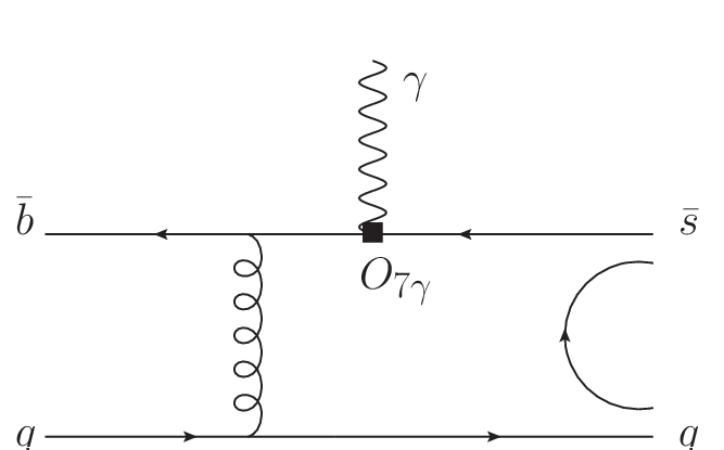
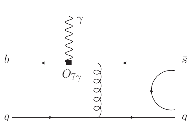
Figure 4: Feynman diagrams from the operator O7​γO_{7\gamma}.

The dominant contributions to the three-body radiative decays B→P​V​γB\to PV\gamma comes from O7​γO_{7\gamma}, whose diagrams are displayed in Fig. 4 with the photon being emitted from the operator. The factorization formulas for the emissions of the right-handed and left-handed photons are written as

ℳ7​γR\displaystyle\mathcal{M}_{7\gamma}^{R} =\displaystyle= −4CFeπmbmB4∫01dx1dz∫0∞b1db1b2db2ϕB(x1,b1)(1−η){[(1+z)ϕt\displaystyle-4C_{F}\frac{e}{\pi}m_{b}m_{B}^{4}\int_{0}^{1}dx_{1}dz\int_{0}^{\infty}b_{1}db_{1}b_{2}db_{2}\phi_{B}(x_{1},b_{1})(1-\eta)\Big\{[(1+z)\phi_{t} (61)
+η(1−2z)(ϕv+ϕa)]Ee(ta)ha(x1,z,b1,b2)+η(ϕv+ϕa)Ee(ta′)ha′(x1,z,b1,b2)},\displaystyle+\sqrt{\eta}(1-2z)(\phi_{v}+\phi_{a})]E_{e}(t_{a})h_{a}(x_{1},z,b_{1},b_{2})+\sqrt{\eta}(\phi_{v}+\phi_{a})E_{e}(t_{a}^{\prime})h_{a}^{\prime}(x_{1},z,b_{1},b_{2})\Big\},
ℳ7​γL\displaystyle\mathcal{M}_{7\gamma}^{L} =\displaystyle= 0,\displaystyle 0, (62)

respectively, where the left-helicity amplitude ℳ7​γL\mathcal{M}_{7\gamma}^{L} vanishes because of the neglect of the strange quark mass.

Refer to caption Refer to caption
Figure 5: Feynman diagrams from the operator O8​gO_{8g}.

The diagrams associated with the operator O8​gO_{8g} are depicted in Fig. 5, where the hard gluon from the operator O8​gO_{8g} kicks the soft spectator, making it an energetic collinear quark, and the photon is emitted via the bremsstrahlung. The amplitudes are written as

ℳ8​gR⁡(a)\displaystyle\mathcal{M}_{8g}^{R(a)} =\displaystyle= 2​CFπmbmB4e∫01dx1dz∫0∞b1db1b2db2ϕB(x1,b1){[(x1−2z)ϕt+3ηz(ϕv+ϕa)]QsEe(tb)\displaystyle\frac{2C_{F}}{\pi}m_{b}m_{B}^{4}e\int_{0}^{1}dx_{1}dz\int_{0}^{\infty}b_{1}db_{1}b_{2}db_{2}\phi_{B}(x_{1},b_{1})\Big\{[(x_{1}-2z)\phi_{t}+3\sqrt{\eta}z(\phi_{v}+\phi_{a})]Q_{s}E_{e}(t_{b}) (63)
×hb(x1,z,b1,b2)−[(1−η+x1)(x1ϕt+ηz(ϕv+ϕa))]QbEe(tb′)hb′(x1,z,b1,b2)},\displaystyle\times h_{b}(x_{1},z,b_{1},b_{2})-[(1-\eta+x_{1})(x_{1}\phi_{t}+\sqrt{\eta}z(\phi_{v}+\phi_{a}))]Q_{b}E_{e}(t_{b}^{\prime})h_{b}^{\prime}(x_{1},z,b_{1},b_{2})\Big\},
ℳ8​gL⁡(a)\displaystyle\mathcal{M}_{8g}^{L(a)} =\displaystyle= 2​CFπmbmB4Qse∫01dx1dz∫0∞b1db1b2db2ϕB(x1,b1){(1−z)(η(2x1−z)ϕt\displaystyle\frac{2C_{F}}{\pi}m_{b}m_{B}^{4}Q_{s}e\int_{0}^{1}dx_{1}dz\int_{0}^{\infty}b_{1}db_{1}b_{2}db_{2}\phi_{B}(x_{1},b_{1})\Big\{(1-z)(\eta(2x_{1}-z)\phi_{t} (64)
+3x1η(ϕv−ϕa))}Ee(tb)hb(x1,z,b1,b2),\displaystyle+3x_{1}\sqrt{\eta}(\phi_{v}-\phi_{a}))\Big\}E_{e}(t_{b})h_{b}(x_{1},z,b_{1},b_{2}),

for the first two diagrams, where Qb⁡(s)Q_{b(s)} labels the charge of the bb (ss) quark in units of the electron charge ee, and as

ℳ8​gR⁡(b)​(Qq)\displaystyle\mathcal{M}_{8g}^{R(b)}(Q_{q}) =\displaystyle= 2​CFπmbmB4Qqe∫01dx1dz∫0∞b1db1b2db2ϕB(x1,b1){−(1−η)[(2+z−2η−x1)ϕt\displaystyle\frac{2C_{F}}{\pi}m_{b}m_{B}^{4}Q_{q}e\int_{0}^{1}dx_{1}dz\int_{0}^{\infty}b_{1}db_{1}b_{2}db_{2}\phi_{B}(x_{1},b_{1})\Big\{-(1-\eta)[(2+z-2\eta-x_{1})\phi_{t} (65)
+3ηz(ϕv+ϕa)]Ee(tc)hc(x1,z,b1,b2)+[(1−η)(x1ϕt+η(x1−z)(ϕv+ϕa))]\displaystyle+3\sqrt{\eta}z(\phi_{v}+\phi_{a})]E_{e}(t_{c})h_{c}(x_{1},z,b_{1},b_{2})+[(1-\eta)(x_{1}\phi_{t}+\sqrt{\eta}(x_{1}-z)(\phi_{v}+\phi_{a}))]
×Ee(tc′)hc′(x1,z,b1,b2)},\displaystyle\times E_{e}(t_{c}^{\prime})h_{c}^{\prime}(x_{1},z,b_{1},b_{2})\Big\},
ℳ8​gL⁡(b)​(Qq)\displaystyle\mathcal{M}_{8g}^{L(b)}(Q_{q}) =\displaystyle= 2​CFπmbmB4Qqe∫01dx1dz∫0∞b1db1b2db2ϕB(x1,b1){[−zη(1+2z−2x1−η)ϕt\displaystyle\frac{2C_{F}}{\pi}m_{b}m_{B}^{4}Q_{q}e\int_{0}^{1}dx_{1}dz\int_{0}^{\infty}b_{1}db_{1}b_{2}db_{2}\phi_{B}(x_{1},b_{1})\Big\{[-z\eta(1+2z-2x_{1}-\eta)\phi_{t} (66)
+3η(1−η)(z−x1)(ϕv−ϕa)]Ee(tc)hc(x1,z,b1,b2)+[(1−η)(η(x1−z)ϕt\displaystyle+3\sqrt{\eta}(1-\eta)(z-x_{1})(\phi_{v}-\phi_{a})]E_{e}(t_{c})h_{c}(x_{1},z,b_{1},b_{2})+[(1-\eta)(\eta(x_{1}-z)\phi_{t}
−ηx1(ϕv−ϕa))]Ee(tc′)hc′(x1,z,b1,b2)},\displaystyle-\sqrt{\eta}x_{1}(\phi_{v}-\phi_{a}))]E_{e}(t_{c}^{\prime})h_{c}^{\prime}(x_{1},z,b_{1},b_{2})\Big\},

for the last two diagrams.

Next we consider the quark loop corrections from the operators OiO_{i}. The operator O1O_{1} does not contribute due to the color mismatch, and the O3∼6O_{3\sim 6} insertions are small compared to the O2O_{2} insertion. Hence, we consider only the O2O_{2} contributions, in which the photon is emitted either by an external quark or from the quark loop.

Refer to caption Refer to caption
Figure 6: Quark-loop diagrams from the operator O2O_{2} with a photon being emitted by an external quark.

The diagrams with the photon being emitted by an external quark are shown in Fig. 6. The effective vertex b¯→s¯​g\bar{b}\to\bar{s}g resulting from the loop integration in the M​S¯\overline{MS} scheme is given by [66]

Iν\displaystyle I^{\nu} =\displaystyle= −g8​π2​[G⁡(mi2,k2,μ)−23]​b¯​Ta​(k2​γν−kν​k̸)​(1−γ5)​s,\displaystyle-\frac{g}{8\pi^{2}}\left[G(m_{i}^{2},k^{2},\mu)-\frac{2}{3}\right]\bar{b}T^{a}(k^{2}\gamma^{\nu}-k^{\nu}\not{k})(1-\gamma_{5})s,
G⁡(mi2,k2,μ)\displaystyle G(m_{i}^{2},k^{2},\mu) =\displaystyle= −∫01dx4x(1−x)log[mi2−x⁡(1−x)​k2−i​ϵμ2],\displaystyle-\int_{0}^{1}dx4x(1-x)\text{log}\left[\frac{m_{i}^{2}-x(1-x)k^{2}-i\epsilon}{\mu^{2}}\right], (67)

where kk is the virtual gluon momentum and mim_{i}, i=u,ci=u,c, are the masses of the quarks in the loop. The amplitudes are written as

ℳ1​iR⁡(a)\displaystyle\mathcal{M}_{1i}^{R(a)} =\displaystyle= CFπ​mB5​Qs​e​∫01d​x1​𝑑z​∫0∞b1​d​b1​b2​d​b2​ϕB​(x1,b1)​[G⁡(mi2,−x1​z​mB2,tb)−23]\displaystyle\frac{C_{F}}{\pi}m_{B}^{5}Q_{s}e\int_{0}^{1}dx_{1}dz\int_{0}^{\infty}b_{1}db_{1}b_{2}db_{2}\phi_{B}(x_{1},b_{1})[G(m_{i}^{2},-x_{1}zm_{B}^{2},t_{b})-\frac{2}{3}] (68)
×z⁡(3​x1​ϕt+η​(z−2​x1)​(ϕv+ϕa))​Ee​(tb)​hb​(x1,z,b1,b2),\displaystyle\times z(3x_{1}\phi_{t}+\sqrt{\eta}(z-2x_{1})(\phi_{v}+\phi_{a}))E_{e}(t_{b})h_{b}(x_{1},z,b_{1},b_{2}),
ℳ1​iL⁡(a)\displaystyle\mathcal{M}_{1i}^{L(a)} =\displaystyle= CFπmB5e∫01dx1dz∫0∞b1db1b2db2ϕB(x1,b1){[G(mi2,−x1zmB2,tb)−23]x1(1−z)\displaystyle\frac{C_{F}}{\pi}m_{B}^{5}e\int_{0}^{1}dx_{1}dz\int_{0}^{\infty}b_{1}db_{1}b_{2}db_{2}\phi_{B}(x_{1},b_{1})\Big\{[G(m_{i}^{2},-x_{1}zm_{B}^{2},t_{b})-\frac{2}{3}]x_{1}(1-z) (69)
×(3ηzϕt+η(2z−x1)(ϕv−ϕa))QsEe(tb)hb(x1,z,b1,b2)−[G(mi2,−x1zmB2,tb′)\displaystyle\times(3\eta z\phi_{t}+\sqrt{\eta}(2z-x_{1})(\phi_{v}-\phi_{a}))Q_{s}E_{e}(t_{b})h_{b}(x_{1},z,b_{1},b_{2})-[G(m_{i}^{2},-x_{1}zm_{B}^{2},t_{b}^{\prime})
−23](z(1−η+x1)(ηzϕt−x1η(ϕv−ϕa)))QbEe(tb′)hb′(x1,z,b1,b2)},\displaystyle-\frac{2}{3}](z(1-\eta+x_{1})(\eta z\phi_{t}-x_{1}\sqrt{\eta}(\phi_{v}-\phi_{a})))Q_{b}E_{e}(t_{b}^{\prime})h_{b}^{\prime}(x_{1},z,b_{1},b_{2})\Big\},

for the first two diagrams, and as

ℳ1​iR⁡(b)​(Qq)\displaystyle\mathcal{M}_{1i}^{R(b)}(Q_{q}) =\displaystyle= −CFπmB5Qqe∫01dx1dz∫0∞b1db1b2db2ϕB(x1,b1){[G(mi2,(z−x1)(1−η)mB2,tc)\displaystyle-\frac{C_{F}}{\pi}m_{B}^{5}Q_{q}e\int_{0}^{1}dx_{1}dz\int_{0}^{\infty}b_{1}db_{1}b_{2}db_{2}\phi_{B}(x_{1},b_{1})\Big\{[G(m_{i}^{2},(z-x_{1})(1-\eta)m_{B}^{2},t_{c}) (70)
−23](1−η)[3(z−x1)(1−η)ϕt+zη(1+2z−η−2x1)(ϕv+ϕa)]Ee(tc)hc(x1,z,b1,b2)\displaystyle-\frac{2}{3}](1-\eta)[3(z-x_{1})(1-\eta)\phi_{t}+z\sqrt{\eta}(1+2z-\eta-2x_{1})(\phi_{v}+\phi_{a})]E_{e}(t_{c})h_{c}(x_{1},z,b_{1},b_{2})
−[G⁡(mi2,(z−x1)​(1−η)​mB2,tc′)−23]​((1−η)2​(x1​ϕt+η​(x1−z)​(ϕv+ϕa)))\displaystyle-[G(m_{i}^{2},(z-x_{1})(1-\eta)m_{B}^{2},t_{c}^{\prime})-\frac{2}{3}]((1-\eta)^{2}(x_{1}\phi_{t}+\sqrt{\eta}(x_{1}-z)(\phi_{v}+\phi_{a})))
×Ee(tc′)hc′(x1,z,b1,b2)},\displaystyle\times E_{e}(t_{c}^{\prime})h_{c}^{\prime}(x_{1},z,b_{1},b_{2})\Big\},
ℳ1​iL⁡(b)​(Qq)\displaystyle\mathcal{M}_{1i}^{L(b)}(Q_{q}) =\displaystyle= −CFπmB5Qqe∫01dx1dz∫0∞b1db1b2db2ϕB(x1,b1){[G(mi2,(z−x1)(1−η)mB2,tc)\displaystyle-\frac{C_{F}}{\pi}m_{B}^{5}Q_{q}e\int_{0}^{1}dx_{1}dz\int_{0}^{\infty}b_{1}db_{1}b_{2}db_{2}\phi_{B}(x_{1},b_{1})\Big\{[G(m_{i}^{2},(z-x_{1})(1-\eta)m_{B}^{2},t_{c}) (71)
−23](1−η)(z−x1)[3ηzϕt−η(2+z−2η−x1)(ϕv−ϕa)]Ee(tc)hc(x1,z,b1,b2)\displaystyle-\frac{2}{3}](1-\eta)(z-x_{1})[3\eta z\phi_{t}-\sqrt{\eta}(2+z-2\eta-x_{1})(\phi_{v}-\phi_{a})]E_{e}(t_{c})h_{c}(x_{1},z,b_{1},b_{2})
+[G⁡(mi2,(z−x1)​(1−η)​mB2,tc′)−23]​[(1−η)​(x1−z)​(η⁡(x1−z)​ϕt−η​x1​(ϕv−ϕa))]\displaystyle+[G(m_{i}^{2},(z-x_{1})(1-\eta)m_{B}^{2},t_{c}^{\prime})-\frac{2}{3}][(1-\eta)(x_{1}-z)(\eta(x_{1}-z)\phi_{t}-\sqrt{\eta}x_{1}(\phi_{v}-\phi_{a}))]
×Ee(tc′)hc′(x1,z,b1,b2)},\displaystyle\times E_{e}(t_{c}^{\prime})h_{c}^{\prime}(x_{1},z,b_{1},b_{2})\Big\},

for the last two diagrams.

Refer to caption Refer to caption
Figure 7: Quark-loop diagrams from the operator O2O_{2} with the photon being emitted from the quark loop.

In the case where the photon is emitted from the quark loop, as displayed in Fig. 7, the sum of the effective vertex b¯→s¯​γ​g∗\bar{b}\to\bar{s}\gamma g^{*} produces [67, 68]

I=b¯​γρ​(1−γ5)2​Ta​s​Iμ​ν​ρ​Aμ​Aa​ν,\displaystyle I=\bar{b}\gamma^{\rho}\frac{(1-\gamma_{5})}{2}T^{a}sI_{\mu\nu\rho}A^{\mu}A^{a\nu}, (72)

where

Iμ​ν​ρ\displaystyle I_{\mu\nu\rho} =\displaystyle= A4​[(q⋅k)​ϵμ​ν​ρ​σ​(q−k)σ+ϵν​ρ​σ​τ​qσ​kτ​kμ−ϵμ​ν​σ​τ​qσ​kτ​qν]\displaystyle A_{4}[(q\cdot k)\epsilon_{\mu\nu\rho\sigma}(q-k)^{\sigma}+\epsilon_{\nu\rho\sigma\tau}q^{\sigma}k^{\tau}k_{\mu}-\epsilon_{\mu\nu\sigma\tau}q^{\sigma}k^{\tau}q_{\nu}] (73)
+A5​[ϵμ​ρ​σ​τ​qσ​kτ​kν−k2​ϵμ​ν​ρ​σ​qτ],\displaystyle+A_{5}[\epsilon_{\mu\rho\sigma\tau}q^{\sigma}k^{\tau}k_{\nu}-k^{2}\epsilon_{\mu\nu\rho\sigma}q^{\tau}],

with

A4\displaystyle A_{4} =\displaystyle= −4​i​e​g3​π2∫01dx∫01−xdyx​yx⁡(1−x)​k2+2​x​y​q⋅k−mi2,\displaystyle-\frac{4ieg}{3\pi^{2}}\int_{0}^{1}dx\int_{0}^{1-x}dy\frac{xy}{x(1-x)k^{2}+2xyq\cdot k-m_{i}^{2}}, (74)
A5\displaystyle A_{5} =\displaystyle= 4​i​e​g3​π2​∫01d​x​∫01−xd​y​x⁡(1−x)x⁡(1−x)​k2+2​x​y​q⋅k−mi2,\displaystyle\frac{4ieg}{3\pi^{2}}\int_{0}^{1}dx\int_{0}^{1-x}dy\frac{x(1-x)}{x(1-x)k^{2}+2xyq\cdot k-m_{i}^{2}}, (75)

qq (kk) being the photon (gluon) momentum. The amplitudes for the two diagrams are expressed as

ℳ2​iR\displaystyle\mathcal{M}_{2i}^{R} =\displaystyle= −83CFπmB5e∫01dx∫01−xdy∫01dx1dz∫0∞b1db1ϕB(x1,b1)αs(td)e−SB​(td)\displaystyle-\frac{8}{3}\frac{C_{F}}{\pi}m_{B}^{5}e\int_{0}^{1}dx\int_{0}^{1-x}dy\int_{0}^{1}dx_{1}dz\int_{0}^{\infty}b_{1}db_{1}\phi_{B}(x_{1},b_{1})\alpha_{s}(t_{d})e^{-S_{B}(t_{d})} (76)
×he′x​y​z​(1−η)​mB2−mi2×(1−η)z{xy[(1−η+2x1)ϕt−η(1−η−z+x1)(ϕv+ϕa)]\displaystyle\times\frac{h_{e}^{\prime}}{xyz(1-\eta)m_{B}^{2}-m_{i}^{2}}\times(1-\eta)z\Big\{xy[(1-\eta+2x_{1})\phi_{t}-\sqrt{\eta}(1-\eta-z+x_{1})(\phi_{v}+\phi_{a})]
−x(1−x)[3x1ϕt+η(z−2x1)(ϕv+ϕa)]},\displaystyle-x(1-x)[3x_{1}\phi_{t}+\sqrt{\eta}(z-2x_{1})(\phi_{v}+\phi_{a})]\Big\},
ℳ2​iL\displaystyle\mathcal{M}_{2i}^{L} =\displaystyle= 83​CFπ​mB5​e​∫01d​x​∫01−xd​y​∫01d​x1​𝑑z​∫0∞b1​d​b1​ϕB​(x1,b1)​αs​(td)​e−SB​(td)\displaystyle\frac{8}{3}\frac{C_{F}}{\pi}m_{B}^{5}e\int_{0}^{1}dx\int_{0}^{1-x}dy\int_{0}^{1}dx_{1}dz\int_{0}^{\infty}b_{1}db_{1}\phi_{B}(x_{1},b_{1})\alpha_{s}(t_{d})e^{-S_{B}(t_{d})} (77)
×he′x​y​z​(1−η)​mB2−mi2×(1−η)z{xy[2ηzϕt+(z−x1)η(ϕv−ϕa)]−x(1−x)\displaystyle\times\frac{h_{e}^{\prime}}{xyz(1-\eta)m_{B}^{2}-m_{i}^{2}}\times(1-\eta)z\Big\{xy[2\eta z\phi_{t}+(z-x_{1})\sqrt{\eta}(\phi_{v}-\phi_{a})]-x(1-x)
×[ηzϕt−x1η(ϕv−ϕa)]},\displaystyle\times[\eta z\phi_{t}-x_{1}\sqrt{\eta}(\phi_{v}-\phi_{a})]\Big\},

in which the function he′h_{e}^{\prime} is defined by

he′=K0​(x1​z​mB​b1)−[θ⁡(B2)​K0​(b1​B2)+θ⁡(−B2)​i​π2​H0(1)​(b1​|B2|)],\displaystyle h_{e}^{\prime}=K_{0}(\sqrt{x_{1}z}m_{B}b_{1})-[\theta(B^{2})K_{0}(b_{1}\sqrt{B^{2}})+\theta(-B^{2})\frac{i\pi}{2}H_{0}^{(1)}(b_{1}\sqrt{|B^{2}|})], (78)

with

B2=x1​z​mB2−y​z​(1−η)1−x​mB2+mi2x⁡(1−x).\displaystyle B^{2}=x_{1}zm_{B}^{2}-\frac{yz(1-\eta)}{1-x}m_{B}^{2}+\frac{m_{i}^{2}}{x(1-x)}. (79)
Refer to caption Refer to caption
Figure 8: Annihilation diagrams.

The annihilation diagrams are exhibited in Fig. 8, to which three types of operators contribute, the left-handed current between b¯\bar{b} and qq quark and the left-handed current between the final state quarks (L​LLL); the left-handed current between b¯\bar{b} and qq quark and the right-handed current between the final state quarks (L​RLR); the (S−P)​(S+P)(S-P)(S+P) current from the Fierz transformation of the (V−A)​(V+A)(V-A)(V+A) operators (SP). Here we define the combinations of the Wilson coefficients:

a1\displaystyle a_{1} =\displaystyle= C2+C1/3,a4=C4+C3/3,a6=C6+C5/3,\displaystyle C_{2}+C_{1}/3,~a_{4}=C_{4}+C_{3}/3,~a_{6}=C_{6}+C_{5}/3,
a8\displaystyle a_{8} =\displaystyle= C8+C7/3,a10=C10+C9/3.\displaystyle C_{8}+C_{7}/3,~a_{10}=C_{10}+C_{9}/3. (80)

The factorization formulas for the annihilation contributions are given by

ℳa​n​nR⁡(a,L​L)​(Qq)\displaystyle\mathcal{M}_{ann}^{R(a,LL)}(Q_{q}) =\displaystyle= 2​6​η​mB3​Qq​e​[(2​ζ−1)​Fv+Fa]​∫01d​x​∫0∞b1​d​b1​ϕB​(x1,b1)\displaystyle 2\sqrt{6\eta}m_{B}^{3}Q_{q}e[(2\zeta-1)F_{v}+F_{a}]\int_{0}^{1}dx\int_{0}^{\infty}b_{1}db_{1}\phi_{B}(x_{1},b_{1}) (81)
×Ea​(te′)​K0​(x1​(1−η)​mB​b1)​(1−η),\displaystyle\times E_{a}(t_{e}^{\prime})K_{0}(\sqrt{x_{1}(1-\eta)}m_{B}b_{1})(1-\eta),
ℳa​n​nL⁡(a,L​L)​(Qq)\displaystyle\mathcal{M}_{ann}^{L(a,LL)}(Q_{q}) =\displaystyle= 26​ηmB3Qbe[(2ζ−1)Fv−Fa)∫01dx∫0∞b1db1ϕB(x1,b1)\displaystyle 2\sqrt{6\eta}m_{B}^{3}Q_{b}e[(2\zeta-1)F_{v}-F_{a})\int_{0}^{1}dx\int_{0}^{\infty}b_{1}db_{1}\phi_{B}(x_{1},b_{1}) (82)
×{Ea​(te)​K0​(1−η+x1​mB​b1)​(1−η+x1)+Ea​(te′)​K0​(x1​(1−η)​mB​b1)​x1},\displaystyle\times\Big\{E_{a}(t_{e})K_{0}(\sqrt{1-\eta+x_{1}}m_{B}b_{1})(1-\eta+x_{1})+E_{a}(t_{e}^{\prime})K_{0}(\sqrt{x_{1}(1-\eta)}m_{B}b_{1})x_{1}\Big\},
ℳa​n​nR⁡(a,L​R)​(Qq)\displaystyle\mathcal{M}_{ann}^{R(a,LR)}(Q_{q}) =\displaystyle= 2​6​η​mB3​Qq​e​[(2​ζ−1)​Fv−Fa]​∫01d​x​∫0∞b1​d​b1​ϕB​(x1,b1)\displaystyle 2\sqrt{6\eta}m_{B}^{3}Q_{q}e[(2\zeta-1)F_{v}-F_{a}]\int_{0}^{1}dx\int_{0}^{\infty}b_{1}db_{1}\phi_{B}(x_{1},b_{1}) (83)
×Ea​(te′)​K0​(x1​(1−η)​mB​b1)​(1−η),\displaystyle\times E_{a}(t_{e}^{\prime})K_{0}(\sqrt{x_{1}(1-\eta)}m_{B}b_{1})(1-\eta),
ℳa​n​nL⁡(a,L​R)​(Qq)\displaystyle\mathcal{M}_{ann}^{L(a,LR)}(Q_{q}) =\displaystyle= 26​ηmB3Qbe[(2ζ−1)Fv+Fa)∫01dx∫0∞b1db1ϕB(x1,b1)\displaystyle 2\sqrt{6\eta}m_{B}^{3}Q_{b}e[(2\zeta-1)F_{v}+F_{a})\int_{0}^{1}dx\int_{0}^{\infty}b_{1}db_{1}\phi_{B}(x_{1},b_{1}) (84)
×{Ea​(te)​K0​(1−η+x1​mB​b1)​(1−η+x1)+Ea​(te′)​K0​(x1​(1−η)​mB​b1)​x1},\displaystyle\times\Big\{E_{a}(t_{e})K_{0}(\sqrt{1-\eta+x_{1}}m_{B}b_{1})(1-\eta+x_{1})+E_{a}(t_{e}^{\prime})K_{0}(\sqrt{x_{1}(1-\eta)}m_{B}b_{1})x_{1}\Big\},
ℳa​n​nR⁡(b,L​L)​(Qq)\displaystyle\mathcal{M}_{ann}^{R(b,LL)}(Q_{q}) =\displaystyle= −ℳa​n​nR,(b,L​R)​(Qq)\displaystyle-\mathcal{M}_{ann}^{R,(b,LR)}(Q_{q}) (85)
=\displaystyle= −26​ηefBmB3∫01dz∫0∞b2db2{Qs(ϕv+ϕa)Ea′(tf)i​π2H0(1)(1−zmBb2)\displaystyle-2\sqrt{6\eta}ef_{B}m_{B}^{3}\int_{0}^{1}dz\int_{0}^{\infty}b_{2}db_{2}\Big\{Q_{s}(\phi_{v}+\phi_{a})E_{a}^{\prime}(t_{f})\frac{i\pi}{2}H_{0}^{(1)}(\sqrt{1-z}m_{B}b_{2})
−Qqz(ϕv+ϕa)Ea′(tf′)i​π2H0(1)(z⁡(1−η)mBb2)},\displaystyle-Q_{q}z(\phi_{v}+\phi_{a})E_{a}^{\prime}(t_{f}^{\prime})\frac{i\pi}{2}H_{0}^{(1)}(\sqrt{z(1-\eta)}m_{B}b_{2})\Big\},
ℳa​n​nL⁡(b,L​L)​(Qq)\displaystyle\mathcal{M}_{ann}^{L(b,LL)}(Q_{q}) =\displaystyle= −ℳa​n​nL,(b,L​R)​(Qq)\displaystyle-\mathcal{M}_{ann}^{L,(b,LR)}(Q_{q}) (86)
=\displaystyle= 26​ηefBmB3∫01dz∫0∞b2db2{Qs(1−z)(ϕv−ϕa)Ea′(tf)i​π2H0(1)(1−zmBb2)\displaystyle 2\sqrt{6\eta}ef_{B}m_{B}^{3}\int_{0}^{1}dz\int_{0}^{\infty}b_{2}db_{2}\Big\{Q_{s}(1-z)(\phi_{v}-\phi_{a})E_{a}^{\prime}(t_{f})\frac{i\pi}{2}H_{0}^{(1)}(\sqrt{1-z}m_{B}b_{2})
−(1−η)Qq(ϕv−ϕa)Ea′(tf′)i​π2H0(1)(z⁡(1−η)mBb2)},\displaystyle-(1-\eta)Q_{q}(\phi_{v}-\phi_{a})E_{a}^{\prime}(t_{f}^{\prime})\frac{i\pi}{2}H_{0}^{(1)}(\sqrt{z(1-\eta)}m_{B}b_{2})\Big\},
ℳa​n​nR⁡(S​P)​(Qq)\displaystyle\mathcal{M}_{ann}^{R(SP)}(Q_{q}) =\displaystyle= 46efBmB3∫01dz∫0∞b2db2{QsϕtEa′(tf)i​π2H0(1)(1−zmBb2)\displaystyle 4\sqrt{6}ef_{B}m_{B}^{3}\int_{0}^{1}dz\int_{0}^{\infty}b_{2}db_{2}\Big\{Q_{s}\phi_{t}E_{a}^{\prime}(t_{f})\frac{i\pi}{2}H_{0}^{(1)}(\sqrt{1-z}m_{B}b_{2}) (87)
+Qq(1−η)ϕtEa′(tf′)i​π2H0(1)(z⁡(1−η)mBb2)},\displaystyle+Q_{q}(1-\eta)\phi_{t}E_{a}^{\prime}(t_{f}^{\prime})\frac{i\pi}{2}H_{0}^{(1)}(\sqrt{z(1-\eta)}m_{B}b_{2})\Big\},
ℳa​n​nL⁡(S​P)​(Qq)\displaystyle\mathcal{M}_{ann}^{L(SP)}(Q_{q}) =\displaystyle= 46efBmB3∫01dz∫0∞b2db2{Qsη(1−z)ϕtEa′(tf)i​π2H0(1)(1−zmBb2)\displaystyle 4\sqrt{6}ef_{B}m_{B}^{3}\int_{0}^{1}dz\int_{0}^{\infty}b_{2}db_{2}\Big\{Q_{s}\eta(1-z)\phi_{t}E_{a}^{\prime}(t_{f})\frac{i\pi}{2}H_{0}^{(1)}(\sqrt{1-z}m_{B}b_{2}) (88)
+QqηzϕtEa′(tf′)i​π2H0(1)(z⁡(1−η)mBb2)}.\displaystyle+Q_{q}\eta z\phi_{t}E_{a}^{\prime}(t_{f}^{\prime})\frac{i\pi}{2}H_{0}^{(1)}(\sqrt{z(1-\eta)}m_{B}b_{2})\Big\}.

Finally, we sum the squared amplitudes for the B+B^{+} meson decays in the helicity basis, |𝒜⁡(B+)|2=∑i=R,L|𝒜i​(B+)|2|\mathcal{A}(B^{+})|^{2}=\sum_{i=R,L}|\mathcal{A}^{i}(B^{+})|^{2}, deriving

𝒜i​(B+)\displaystyle\mathcal{A}^{i}(B^{+}) =\displaystyle= GF2​Vu​b∗​Vu​s​{C2​(ℳ1​ui⁡(a)+ℳ1​ui⁡(b)​(Qu)+ℳ2​ui)+a1​(ℳa​n​ni⁡(a,L​L)​(Qu)+ℳa​n​ni⁡(b,L​L)​(Qu))}\displaystyle\frac{G_{F}}{\sqrt{2}}V_{ub}^{*}V_{us}\Big\{C_{2}\left(\mathcal{M}_{1u}^{i(a)}+\mathcal{M}_{1u}^{i(b)}(Q_{u})+\mathcal{M}_{2u}^{i}\right)+a_{1}\left(\mathcal{M}_{ann}^{i(a,LL)}(Q_{u})+\mathcal{M}_{ann}^{i(b,LL)}(Q_{u})\right)\Big\} (89)
+\displaystyle+ GF2​Vc​b∗​Vc​s​{C2​(ℳ1​ci⁡(a)+ℳ1​ci⁡(b)​(Qu)+ℳ2​ci)}\displaystyle\frac{G_{F}}{\sqrt{2}}V_{cb}^{*}V_{cs}\Big\{C_{2}\left(\mathcal{M}_{1c}^{i(a)}+\mathcal{M}_{1c}^{i(b)}(Q_{u})+\mathcal{M}_{2c}^{i}\right)\Big\}
−\displaystyle- GF2Vt​b∗Vt​s{C7​γℳ7​γi+C8​g(ℳ8​gi⁡(a)+ℳ8​gi⁡(b)(Qu))\displaystyle\frac{G_{F}}{\sqrt{2}}V_{tb}^{*}V_{ts}\Big\{C_{7\gamma}\mathcal{M}_{7\gamma}^{i}+C_{8g}\left(\mathcal{M}_{8g}^{i(a)}+\mathcal{M}_{8g}^{i(b)}(Q_{u})\right)
+\displaystyle+ (a4+a10)(ℳa​n​ni⁡(a,L​L)(Qu)+ℳa​n​ni⁡(b,L​L)(Qu))+(a6+a8)ℳa​n​ni⁡(S​P)(Qu)}.\displaystyle(a_{4}+a_{10})\left(\mathcal{M}_{ann}^{i(a,LL)}(Q_{u})+\mathcal{M}_{ann}^{i(b,LL)}(Q_{u})\right)+(a_{6}+a_{8})\mathcal{M}_{ann}^{i(SP)}(Q_{u})\Big\}.

We have the similar sum for the B0B^{0} meson decay amplitudes with

𝒜i​(B0)\displaystyle\mathcal{A}^{i}(B^{0}) =\displaystyle= GF2​Vu​b∗​Vu​s​{C2​(ℳ1​ui⁡(a)+ℳ1​ui⁡(b)​(Qd)+ℳ2​ui)}\displaystyle\frac{G_{F}}{\sqrt{2}}V_{ub}^{*}V_{us}\Big\{C_{2}\left(\mathcal{M}_{1u}^{i(a)}+\mathcal{M}_{1u}^{i(b)}(Q_{d})+\mathcal{M}_{2u}^{i}\right)\Big\} (90)
+\displaystyle+ GF2​Vc​b∗​Vc​s​{C2​(ℳ1​ci⁡(a)+ℳ1​ci⁡(b)​(Qd)+ℳ2​ci)}\displaystyle\frac{G_{F}}{\sqrt{2}}V_{cb}^{*}V_{cs}\Big\{C_{2}\left(\mathcal{M}_{1c}^{i(a)}+\mathcal{M}_{1c}^{i(b)}(Q_{d})+\mathcal{M}_{2c}^{i}\right)\Big\}
−\displaystyle- GF2Vt​b∗Vt​s{C7​γℳ7​γi+C8​g(ℳ8​gi⁡(a)+ℳ8​gi⁡(b)(Qd))\displaystyle\frac{G_{F}}{\sqrt{2}}V_{tb}^{*}V_{ts}\Big\{C_{7\gamma}\mathcal{M}_{7\gamma}^{i}+C_{8g}\left(\mathcal{M}_{8g}^{i(a)}+\mathcal{M}_{8g}^{i(b)}(Q_{d})\right)
+\displaystyle+ (a4−12a10)(ℳa​n​ni⁡(a,L​L)(Qd)+ℳa​n​ni⁡(b,L​L)(Qd))+(a6−12a8)ℳa​n​ni⁡(S​P)(Qd)}.\displaystyle(a_{4}-\frac{1}{2}a_{10})\left(\mathcal{M}_{ann}^{i(a,LL)}(Q_{d})+\mathcal{M}_{ann}^{i(b,LL)}(Q_{d})\right)+(a_{6}-\frac{1}{2}a_{8})\mathcal{M}_{ann}^{i(SP)}(Q_{d})\Big\}.

It is seen that the O7​γO_{7\gamma} contributions to the B+B^{+} and B0B^{0} meson decays are identical.

The explicit expressions for some functions appearing in the above factorization formulas are presented below. We adopt the model

ϕB​(x,b)=NB​x2​(1−x)2​exp​[−12​(x​mBωB)2−12​(ωB​b)2],\displaystyle\phi_{B}(x,b)=N_{B}x^{2}(1-x)^{2}\text{exp}\left[-\frac{1}{2}(\frac{xm_{B}}{\omega_{B}})^{2}-\frac{1}{2}(\omega_{B}b)^{2}\right], (91)

for the BB meson DA, where bb is the impact parameter conjugate to the spectator transverse momentum kTk_{T}, NBN_{B} is the normalization constant, and the shape parameter ωB=0.40±0.04\omega_{B}=0.40\pm 0.04 GeV has been determined through the study of the BB meson transition form factors [43, 44].

The hard scales are chosen as

ta\displaystyle t_{a} =\displaystyle= max⁡{z​mB,1/b1,1/b2},\displaystyle{\rm max}\{\sqrt{z}m_{B},1/b_{1},1/b_{2}\},
ta′\displaystyle t_{a}^{\prime} =\displaystyle= max⁡{|x1−η|​mB,z​x1​mB,1/b1,1/b2},\displaystyle{\rm max}\{\sqrt{|x_{1}-\eta|}m_{B},\sqrt{zx_{1}}m_{B},1/b_{1},1/b_{2}\},
tb\displaystyle t_{b} =\displaystyle= max⁡{1−z​mB,z​x1​mB,1/b1,1/b2},\displaystyle{\rm max}\{\sqrt{1-z}m_{B},\sqrt{zx_{1}}m_{B},1/b_{1},1/b_{2}\},
tb′\displaystyle t_{b}^{\prime} =\displaystyle= max⁡{1+x1−η​mB,z​x1​mB,1/b1,1/b2},\displaystyle{\rm max}\{\sqrt{1+x_{1}-\eta}m_{B},\sqrt{zx_{1}}m_{B},1/b_{1},1/b_{2}\},
tc\displaystyle t_{c} =\displaystyle= max⁡{z⁡(1−η)​mB,|(x1−z)​(1−η)|​mB,1/b1,1/b2},\displaystyle{\rm max}\{\sqrt{z(1-\eta)}m_{B},\sqrt{|(x_{1}-z)(1-\eta)|}m_{B},1/b_{1},1/b_{2}\},
tc′\displaystyle t_{c}^{\prime} =\displaystyle= max⁡{x1​(1−η)​mB,|(x1−z)​(1−η)|​mB,1/b1,1/b2},\displaystyle{\rm max}\{\sqrt{x_{1}(1-\eta)}m_{B},\sqrt{|(x_{1}-z)(1-\eta)|}m_{B},1/b_{1},1/b_{2}\},
td\displaystyle t_{d} =\displaystyle= max⁡{x1​z​mB,|B2|,1/b1},\displaystyle{\rm max}\{\sqrt{x_{1}z}m_{B},\sqrt{|B^{2}|},1/b_{1}\},
te\displaystyle t_{e} =\displaystyle= max⁡{1−η+x1​mB,1/b1},te′=max⁡{x1​(1−η)​mB,1/b1},\displaystyle{\rm max}\{\sqrt{1-\eta+x_{1}}m_{B},1/b_{1}\},\quad t_{e}^{\prime}={\rm max}\{\sqrt{x_{1}(1-\eta)}m_{B},1/b_{1}\},
tf\displaystyle t_{f} =\displaystyle= max⁡{1−z​mB,1/b2},tf′=max⁡{z⁡(1−η)​mB,1/b2}.\displaystyle{\rm max}\{\sqrt{1-z}m_{B},1/b_{2}\},\quad t_{f}^{\prime}={\rm max}\{\sqrt{z(1-\eta)}m_{B},1/b_{2}\}. (92)

The hard functions are written as

ha​(x1,z,b1,b2)\displaystyle h_{a}(x_{1},z,b_{1},b_{2}) =\displaystyle= K0​(z​x1​mB​b1)​[θ⁡(b1−b2)​K0​(z​mB​b1)​I0​(z​mB​b2)+(b1↔b2)]​St​(z),\displaystyle K_{0}(\sqrt{zx_{1}}m_{B}b_{1})[\theta(b_{1}-b_{2})K_{0}(\sqrt{z}m_{B}b_{1})I_{0}(\sqrt{z}m_{B}b_{2})+(b_{1}\leftrightarrow b_{2})]S_{t}(z),
ha′​(x1,z,b1,b2)\displaystyle h_{a}^{\prime}(x_{1},z,b_{1},b_{2}) =\displaystyle= K0​(z​x1​mB​b2)​St​(x1)\displaystyle K_{0}(\sqrt{zx_{1}}m_{B}b_{2})S_{t}(x_{1})
×{i​π2​[θ⁡(b2−b1)​H0(1)​(|x1−η|​mB​b2)​J0​(|x1−η|​mB​b1)+(b2↔b1)],x1<η,θ⁡(b2−b1)​K0​(x1−η​mB​b2)​I0​(x1−η​mB​b1)+(b2↔b1),x1>η,\displaystyle\times\{\begin{array}[]{ll}\frac{i\pi}{2}[\theta(b_{2}-b_{1})H_{0}^{(1)}(\sqrt{|x_{1}-\eta|}m_{B}b_{2})J_{0}(\sqrt{|x_{1}-\eta|}m_{B}b_{1})+(b_{2}\leftrightarrow b_{1})],&x_{1}<\eta,\\ \theta(b_{2}-b_{1})K_{0}(\sqrt{x_{1}-\eta}m_{B}b_{2})I_{0}(\sqrt{x_{1}-\eta}m_{B}b_{1})+(b_{2}\leftrightarrow b_{1}),&x_{1}>\eta,\end{array}
hb​(x1,z,b1,b2)\displaystyle h_{b}(x_{1},z,b_{1},b_{2}) =\displaystyle= K0​(x1​z​mB​b1)​i​π2​[θ⁡(b1−b2)​H0(1)​(1−z​mB​b1)​J0​(1−z​mB​b2)+(b2↔b1)]​St​(z),\displaystyle K_{0}(\sqrt{x_{1}z}m_{B}b_{1})\frac{i\pi}{2}[\theta(b_{1}-b_{2})H_{0}^{(1)}(\sqrt{1-z}m_{B}b_{1})J_{0}(\sqrt{1-z}m_{B}b_{2})+(b_{2}\leftrightarrow b_{1})]S_{t}(z),
hb′​(x1,z,b1,b2)\displaystyle h_{b}^{\prime}(x_{1},z,b_{1},b_{2}) =\displaystyle= K0(x1​zmBb2)St(x1)[θ(b2−b1)K0(1+x1−ηmBb2)I0(1+x1−ηmBb1)\displaystyle K_{0}(\sqrt{x_{1}z}m_{B}b_{2})S_{t}(x_{1})[\theta(b_{2}-b_{1})K_{0}(\sqrt{1+x_{1}-\eta}m_{B}b_{2})I_{0}(\sqrt{1+x_{1}-\eta}m_{B}b_{1})
+(b2↔b1)],\displaystyle+(b_{2}\leftrightarrow b_{1})],
hc​(x1,z,b1,b2)\displaystyle h_{c}(x_{1},z,b_{1},b_{2}) =\displaystyle= i​π2​[θ⁡(b1−b2)​H0(1)​(z⁡(1−η)​mB​b1)​J0​(z⁡(1−η)​mB​b2)+(b2↔b1)]​St​(z)\displaystyle\frac{i\pi}{2}[\theta(b_{1}-b_{2})H_{0}^{(1)}(\sqrt{z(1-\eta)}m_{B}b_{1})J_{0}(\sqrt{z(1-\eta)}m_{B}b_{2})+(b_{2}\leftrightarrow b_{1})]S_{t}(z)
×{i​π2​H0(1)​(|(x1−z)​(1−η)|​mB​b1),x1<z,K0​((x1−z)​(1−η)​mB​b1),x1>z,\displaystyle\times\{\begin{array}[]{ll}\frac{i\pi}{2}H_{0}^{(1)}(\sqrt{|(x_{1}-z)(1-\eta)|}m_{B}b_{1}),&x_{1}<z,\\ K_{0}(\sqrt{(x_{1}-z)(1-\eta)}m_{B}b_{1}),&x_{1}>z,\end{array}
hc′​(x1,z,b1,b2)\displaystyle h_{c}^{\prime}(x_{1},z,b_{1},b_{2}) =\displaystyle= [θ⁡(b2−b1)​K0​(x1​(1−η)​mB​b2)​I0​(x1​(1−η)​mB​b1)+(b2↔b1)]​St​(x1)\displaystyle[\theta(b_{2}-b_{1})K_{0}(\sqrt{x_{1}(1-\eta)}m_{B}b_{2})I_{0}(\sqrt{x_{1}(1-\eta)}m_{B}b_{1})+(b_{2}\leftrightarrow b_{1})]S_{t}(x_{1})
×{i​π2​H0(1)​(|(x1−z)​(1−η)|​mB​b2),x1<η,K0​((x1−z)​(1−η)​mB​b2),x1>z.\displaystyle\times\{\begin{array}[]{ll}\frac{i\pi}{2}H_{0}^{(1)}(\sqrt{|(x_{1}-z)(1-\eta)|}m_{B}b_{2}),&x_{1}<\eta,\\ K_{0}(\sqrt{(x_{1}-z)(1-\eta)}m_{B}b_{2}),&x_{1}>z.\end{array}

The Sudakov factor St​(x)S_{t}(x) from the threshold resummation follows the parametrization in [69]

St​(x)=21+2​a​Γ​(3/2+a)π​Γ​(1+a)​[x⁡(1−x)]a,\displaystyle S_{t}(x)=\frac{2^{1+2a}\Gamma(3/2+a)}{\sqrt{\pi}\Gamma(1+a)}[x(1-x)]^{a}, (99)

with the parameter a=0.4a=0.4. The evolution factors are given by

Ee​(t)\displaystyle E_{e}(t) =\displaystyle= αs​(t)​exp​[−SB​(t)−S2​(t)],\displaystyle\alpha_{s}(t){\rm exp}[-S_{B}(t)-S_{2}(t)],
Ea​(t)\displaystyle E_{a}(t) =\displaystyle= St​(x1)​exp​[−SB​(t)],Ea′​(t)=St​(z)​exp​[−S2​(t)],\displaystyle S_{t}(x_{1}){\rm exp}[-S_{B}(t)],\quad E_{a}^{\prime}(t)=S_{t}(z){\rm exp}[-S_{2}(t)], (100)

with the Sudakov exponents

SB​(t)\displaystyle S_{B}(t) =\displaystyle= s⁡(x1​mB2,b1)+53​∫1/b1td​μ¯μ¯​γq​(αs​(μ¯)),\displaystyle s(x_{1}\frac{m_{B}}{\sqrt{2}},b_{1})+\frac{5}{3}\int_{1/b_{1}}^{t}\frac{d\bar{\mu}}{\bar{\mu}}\gamma_{q}(\alpha_{s}(\bar{\mu})),
S2​(t)\displaystyle S_{2}(t) =\displaystyle= s⁡(z​mB2,b2)+s⁡((1−z)​mB2,b2)+2​∫1/b2td​μ¯μ¯​γq​(αs​(μ¯)),\displaystyle s(z\frac{m_{B}}{\sqrt{2}},b_{2})+s((1-z)\frac{m_{B}}{\sqrt{2}},b_{2})+2\int_{1/b_{2}}^{t}\frac{d\bar{\mu}}{\bar{\mu}}\gamma_{q}(\alpha_{s}(\bar{\mu})), (101)

γq=−αs/π\gamma_{q}=-\alpha_{s}/\pi being the quark anomalous dimension. The function s⁡(Q,b)s(Q,b) is expressed as

s⁡(Q,b)\displaystyle s(Q,b) =\displaystyle= A(1)2​β1​q^​ln​(q^b^)−A(1)2​β1​(q^−b^)+A(2)4​β12​q^​ln​(q^b^−1)\displaystyle\frac{A^{(1)}}{2\beta_{1}}\hat{q}\text{ln}\big(\frac{\hat{q}}{\hat{b}}\big)-\frac{A^{(1)}}{2\beta_{1}}(\hat{q}-\hat{b})+\frac{A^{(2)}}{4\beta_{1}^{2}}\hat{q}\text{ln}\big(\frac{\hat{q}}{\hat{b}}-1\big) (102)
−\displaystyle- [A(2)4​β12−A(1)4​β1​ln​(e2​γE−12)]​ln​(q^b^),\displaystyle\big[\frac{A^{(2)}}{4\beta_{1}^{2}}-\frac{A^{(1)}}{4\beta_{1}}\text{ln}\big(\frac{e^{2\gamma_{E}-1}}{2}\big)\big]\text{ln}\big(\frac{\hat{q}}{\hat{b}}\big),

where

q^\displaystyle\hat{q} =\displaystyle= ln​Q2​ΛQCD,b^=ln​1b​ΛQCD,\displaystyle\text{ln}\frac{Q}{\sqrt{2}\Lambda_{\rm QCD}},\quad\hat{b}=\text{ln}\frac{1}{b\Lambda_{\rm QCD}},
β1\displaystyle\beta_{1} =\displaystyle= 33−2​nf12,β2=153−19​nf24,\displaystyle\frac{33-2n_{f}}{12},\quad\beta_{2}=\frac{153-19n_{f}}{24},
A(1)\displaystyle A^{(1)} =\displaystyle= 43,A(2)=679−π23−1027​nf+83​β1​ln​(12​eγE),\displaystyle\frac{4}{3},\quad A^{(2)}=\frac{67}{9}-\frac{\pi^{2}}{3}-\frac{10}{27}n_{f}+\frac{8}{3}\beta_{1}\text{ln}\big(\frac{1}{2}e^{\gamma_{E}}\big), (103)

nfn_{f} being the number of the quark flavor, and γE\gamma_{E} the Eular constant.

References

  • [1] J. P. Lees et al. [BaBar Collaboration], Phys. Rev. D 85, 112010 (2012) [arXiv:1201.5897 [hep-ex]].
  • [2] J. P. Lees et al. [BaBar Collaboration], Phys. Rev. D 85, 054023 (2012) [arXiv:1111.3636 [hep-ex]].
  • [3] B. Aubert et al. [BaBar Collaboration], Phys. Rev. D 80, 112001 (2009) [arXiv:0905.3615 [hep-ex]].
  • [4] J. P. Lees et al. [BaBar Collaboration], Phys. Rev. D 83, 112010 (2011) [arXiv:1105.0125 [hep-ex]].
  • [5] B. Aubert et al. [BaBar Collaboration], Phys. Rev. D 79, 072006 (2009) [arXiv:0902.2051 [hep-ex]].
  • [6] B. Aubert et al. [BaBar Collaboration], Phys. Rev. D 78, 012004 (2008) [arXiv:0803.4451 [hep-ex]].
  • [7] A. Garmash et al. [Belle Collaboration], Phys. Rev. D 71, 092003 (2005) [hep-ex/0412066].
  • [8] A. Garmash et al. [Belle Collaboration], Phys. Rev. D 75, 012006 (2007) [hep-ex/0610081].
  • [9] P. Chang et al. [Belle Collaboration], Phys. Lett. B 599, 148 (2004) [hep-ex/0406075].
  • [10] A. Garmash et al. [Belle Collaboration], Phys. Rev. Lett. 96, 251803 (2006) [hep-ex/0512066].
  • [11] R. Aaij et al. [LHCb Collaboration], Phys. Rev. Lett. 111, 101801 (2013) [arXiv:1306.1246 [hep-ex]].
  • [12] R. Aaij et al. [LHCb Collaboration], Phys. Rev. Lett. 112, no. 1, 011801 (2014) [arXiv:1310.4740 [hep-ex]].
  • [13] R. Aaij et al. [LHCb Collaboration], Phys. Rev. D 90, no. 11, 112004 (2014) [arXiv:1408.5373 [hep-ex]].
  • [14] T. Aushev et al., arXiv:1002.5012 [hep-ex].
  • [15] C. H. Chen and H. n. Li, Phys. Lett. B 561, 258 (2003) [hep-ph/0209043].
  • [16] W. F. Wang, H. C. Hu, H. n. Li and C. D. L¨¹, Phys. Rev. D 89, no. 7, 074031 (2014) [arXiv:1402.5280 [hep-ph]].
  • [17] W. F. Wang, H. n. Li, W. Wang and C. D. L¨¹, Phys. Rev. D 91, no. 9, 094024 (2015) [arXiv:1502.05483 [hep-ph]].
  • [18] W. F. Wang and H. n. Li, Phys. Lett. B 763, 29 (2016) [arXiv:1609.04614 [hep-ph]].
  • [19] Z. T. Wei, hep-ph/0301174.
  • [20] B. El-Bennich, A. Furman, R. Kaminski, L. Lesniak, B. Loiseau and B. Moussallam, Phys. Rev. D 79, 094005 (2009) Erratum: [Phys. Rev. D 83, 039903 (2011)] [arXiv:0902.3645 [hep-ph]].
  • [21] S. Krnkl, T. Mannel and J. Virto, Nucl. Phys. B 899, 247 (2015) [arXiv:1505.04111 [hep-ph]].
  • [22] A. Furman, R. Kaminski, L. Lesniak and B. Loiseau, Phys. Lett. B 622, 207 (2005) [hep-ph/0504116].
  • [23] H. Y. Cheng and K. C. Yang, Phys. Rev. D 66, 054015 (2002) [hep-ph/0205133].
  • [24] H. Y. Cheng, C. K. Chua and A. Soni, Phys. Rev. D 76, 094006 (2007) [arXiv:0704.1049 [hep-ph]].
  • [25] M. Diehl, T. Gousset, B. Pire and O. Teryaev, Phys. Rev. Lett. 81, 1782 (1998) [hep-ph/9805380].
  • [26] M. V. Polyakov, Nucl. Phys. B 555, 231 (1999) [hep-ph/9809483].
  • [27] D. M¨¹ller, D. Robaschik, B. Geyer, F.-M. Dittes, J. Horejsi, Fortsch. Phys. 42, 101 (1994) [hep-ph/9812448].
  • [28] M. Diehl, T. Gousset and B. Pire, Phys. Rev. D 62, 073014 (2000) [hep-ph/0003233].
  • [29] H. Sahoo et al. [Belle Collaboration], Phys. Rev. D 84, 071101 (2011) [arXiv:1104.5590 [hep-ex]].
  • [30] M. Gronau and D. Pirjol, Phys. Rev. D 96, no. 1, 013002 (2017) [arXiv:1704.05280 [hep-ph]].
  • [31] B. Aubert et al. [BaBar Collaboration], Phys. Rev. D 75, 051102 (2007) [hep-ex/0611037].
  • [32] C. H. Chen and H. n. Li, Phys. Rev. D 70, 054006 (2004) [hep-ph/0404097].
  • [33] S. Nishida et al. [Belle Collaboration], Phys. Rev. Lett. 89, 231801 (2002) [hep-ex/0205025].
  • [34] P. del Amo Sanchez et al. [BaBar Collaboration], Phys. Rev. D 93, no. 5, 052013 (2016) [arXiv:1512.03579 [hep-ex]].
  • [35] Y. Li, A. J. Ma, W. F. Wang and Z. J. Xiao, Phys. Rev. D 95, no. 5, 056008 (2017) [arXiv:1612.05934 [hep-ph]].
  • [36] A. J. Ma, Y. Li, W. F. Wang and Z. J. Xiao, arXiv:1701.01844 [hep-ph].
  • [37] G. P. Lepage and S. J. Brodsky, Phys. Lett. 87B, 359 (1979).
  • [38] A. V. Efremov and A. V. Radyushkin, Phys. Lett. 94B, 245 (1980).
  • [39] M. Diehl, T. Feldmann, P. Kroll and C. Vogt, Phys. Rev. D 61, 074029 (2000) [hep-ph/9912364].
  • [40] T. Huang, X. H. Wu and M. Z. Zhou, Phys. Rev. D 70, 014013 (2004) [hep-ph/0402100].
  • [41] K. C. Yang, Nucl. Phys. B 776, 187 (2007) [arXiv:0705.0692 [hep-ph]].
  • [42] H. Y. Cheng and K. C. Yang, Phys. Rev. D 78, 094001 (2008) Erratum: [Phys. Rev. D 79, 039903 (2009)] [arXiv:0805.0329 [hep-ph]].
  • [43] Y. Y. Keum, H. n. Li and A. I. Sanda, Phys. Lett. B 504, 6 (2001) [hep-ph/0004004].
  • [44] Y. Y. Keum, H. N. Li and A. I. Sanda, Phys. Rev. D 63, 054008 (2001) [hep-ph/0004173].
  • [45] Y. Y. Keum and H. n. Li, Phys. Rev. D 63, 074006 (2001) [hep-ph/0006001].
  • [46] Y. Y. Keum, M. Matsumori and A. I. Sanda, Phys. Rev. D 72, 014013 (2005) [hep-ph/0406055].
  • [47] C. D. Lu, M. Matsumori, A. I. Sanda and M. Z. Yang, Phys. Rev. D 72, 094005 (2005) Erratum: [Phys. Rev. D 73, 039902 (2006)] [hep-ph/0508300].
  • [48] W. Wang, R. H. Li and C. D. Lu, arXiv:0711.0432 [hep-ph].
  • [49] C. Patrignani et al. [Particle Data Group], Chin. Phys. C 40, no. 10, 100001 (2016).
  • [50] M. Suzuki, Phys. Rev. D 47, 1252 (1993).
  • [51] L. Burakovsky and J. T. Goldman, Phys. Rev. D 56, R1368 (1997) [hep-ph/9703274].
  • [52] H. Y. Cheng, Phys. Rev. D 67, 094007 (2003) [hep-ph/0301198].
  • [53] K. C. Yang, Phys. Rev. D 84, 034035 (2011) [arXiv:1011.6113 [hep-ph]].
  • [54] H. Hatanaka and K. C. Yang, Phys. Rev. D 77, 094023 (2008) Erratum: [Phys. Rev. D 78, 059902 (2008)] [arXiv:0804.3198 [hep-ph]].
  • [55] A. Tayduganov, E. Kou and A. Le Yaouanc, Phys. Rev. D 85, 074011 (2012) [arXiv:1111.6307 [hep-ph]].
  • [56] F. Divotgey, L. Olbrich and F. Giacosa, Eur. Phys. J. A 49, 135 (2013) [arXiv:1306.1193 [hep-ph]].
  • [57] R. J. Dowdall, C. T. H. Davies, R. R. Horgan, C. J. Monahan and J. Shigemitsu Phys. Rev. Lett. 110, no.22, 222003 (2013).
  • [58] F. Bernardoni et al. [ALPHA Collaboration], Phys. Lett. B 735, 349 (2014)
  • [59] H. K. Sun and M. Z. Yang, Phys. Rev. D 95, no.11, 113001 (2017).
  • [60] M. J. Baker, J. Bordes, C. A. Dominguez, J. Penarrocha and K. Schilcher JHEP 1407, 032 (2014).
  • [61] D. Atwood, M. Gronau and A. Soni, Phys. Rev. Lett. 79, 185 (1997) [hep-ph/9704272].
  • [62] M. Gronau and D. Pirjol, Phys. Rev. D 66, 054008 (2002) [hep-ph/0205065].
  • [63] E. Kou, A. Le Yaouanc and A. Tayduganov, Phys. Rev. D 83, 094007 (2011) [arXiv:1011.6593 [hep-ph]].
  • [64] M. Matsumori and A. I. Sanda, Phys. Rev. D 73, 114022 (2006) [hep-ph/0512175].
  • [65] G. Buchalla, A. J. Buras and M. E. Lautenbacher, Rev. Mod. Phys. 68, 1125 (1996) [hep-ph/9512380].
  • [66] M. Bander, D. Silverman and A. Soni, Phys. Rev. Lett. 43, 242 (1979).
  • [67] J. Liu and Y. P. Yao, Phys. Rev. D 42, 1485 (1990).
  • [68] H. Simma and D. Wyler, Nucl. Phys. B 344, 283 (1990).
  • [69] H. n. Li and K. Ukai, Phys. Lett. B 555, 197 (2003) [hep-ph/0211272].