Haar wavelet quasilinearization technique for doubly singular boundary value problems

Randhir Singh, Himanshu Garg and Apoorv Garg ^* Department of Mathematics, Birla Institute of Technology Mesra, India. ^†^†thanks: Corresponding author. E-mail:˜randhir.math@gmail.com ^†^†thanks: E-mail:˜himanshugargcse@gmail.com ^†^†thanks: E-mail:˜apoorv.garg.cse15@gmail.com Affiliation: Department of Computer Science Engineering, Birla Institute of Technology Mesra, India.

Abstract

The Haar wavelet based quasilinearization technique for solving a general class of singular boundary value problems is proposed. Quasilinearization technique is used to linearize nonlinear singular problem. Second rate of convergence is obtained of a sequence of linear singular problems. Numerical solution of linear singular problems is obtained by Haar-wavelet method. In each iteration of quasilinearization technique, the numerical solution is updated by the Haar wavelet method. Convergence analysis of Haar wavelet method is discussed. The results are compared with the results obtained by the other technique and with exact solution. Eight singular problems are solved to show the applicability of the Haar wavelet quasilinearization technique.

Keyword: Doubly singular boundary value problem; Haar Wavelet; Quasilinearization; Lane-Emden equation; Convergence analysis; Green’s function

1 Introduction

In this paper, we consider the following class of nonlinear doubly singular boundary value problems (DSBVPs) [1, 2, 3]

\displaystyle(p(x)y^{\prime}(x))^{\prime}=q(x)f(x,y(x)),~~~~~~~~0<x<1,

(1.1)

with Dirichlet boundary conditions (BCs.)

\displaystyle y(0)=\alpha_{1},~~~y(1)=\beta_{1},

(1.2)

and Neumann-Robin BCs.

\displaystyle y^{\prime}(0)=0,~~~\alpha_{2}\;y(1)+\beta_{2}\;y^{\prime}(1)=\gamma_{2},

(1.3)

where $\alpha_{1}$ , $\beta_{1}$ , $\alpha_{2}$ , $\beta_{2}$ and $\gamma_{2}$ are any real constants. Here, $p(0)=0$ and $q(x)$ may be discontinuous at $x=0$ . Throughout this paper, the following conditions are assumed on $p(x)$ , $q(x)$ and $f(x,y)$ :

: $(C_{1})$ $p(x)\in C[0,1]\cap C^{1}(0,1]$ and $p(x)>0,~q(x)>0\in(0,1]$ .
: $(C_{2})$ $\displaystyle\frac{1}{p(x)}\in L^{1}(0,1]$ and $\displaystyle\int\limits_{0}^{1}\frac{1}{p(x)}\int\limits_{x}^{1}q(s)ds\;dx<\infty$ . (for boundary conditions (1.2))
: $(C_{3})$ $q(x)\in L^{1}(0,1]$ and $\displaystyle\int\limits_{0}^{1}\frac{1}{p(x)}\int\limits_{0}^{x}q(s)ds\;dx<\infty$ . (for boundary conditions (1.3))
: $(C_{4})$ $f(x,y),~f_{y}(x,y)\in C(\Omega)$ and $f_{y}(x,y)\geq 0$ on $\Omega$ , where $\Omega:=\{(0,1]\times\mathbb{R}\}$ .

The well known Thomas-Fermi equations [4, 5], is modeled by the problem (1.1), where $p(x)=1$ , $q(x)=x^{-\frac{1}{2}}$ and $f=y^{\frac{3}{2}}.$ The problem (1.1), where $p(x)=q(x)=x^{2}$ arises in oxygen diffusion in a spherical cell [6, 7] with $f$ of the form

f(x,y)=\frac{ny}{y+k},~~n>0,~~k>0,

and in modelling of heat conduction in human head [8, 9, 10] with $f$ of the form

f(x,y)=-\delta e^{-\theta y},~~~\theta>0,~~~\delta>0.

Existence and uniqueness of doubly singular boundary value problems (1.1) with BCs. (1.2) and (1.3) can be found in [11, 12, 1, 13]. In general, such singular problems are difficult to solve due its singular behavior at $x=0$ . There are several techniques to solve doubly singular boundary value problems (1.1) with BCs. (1.3) where $p(x)=q(x)=x^{\alpha}$ for $\alpha>0$ or $0<\alpha<1$ . The numerical study of doubly singular boundary value problems has been carried out for past couple of decades and still it is an active area of research to develop some better numerical schemes. So far various numerical methods such as the collocation methods [14, 15], tangent chord method [10], finite difference methods [16, 17, 18], spline finite difference methods [19], B-Spline method [20], spline method [21], Chebyshev economization method [22], Cubic spline method [23, 24, 25], Adomian decomposition method (ADM) and modified ADM [26, 27, 28, 29, 30], ADM with Green’s function [31, 32], variational iteration method (VIM) [33, 34, 35], the optimal modified VIM [36], homotopy analysis method [37, 38] and homotopy perturbation method [39] and the references cited therein.

In the recent years the Haar wavelet technique has been popular in the field of numerical approximations. The basic idea of the Haar wavelets and its applications can be found in [40, 41, 42, 43, 44, 45, 46, 47, 48]. The Haar wavelets have gained popularity among researchers for their useful properties such as simple applicability, orthogonality and compact support. Compact support of the Haar wavelet basis permits straight inclusion of the different types of boundary conditions in the numeric algorithms. Due to the linear and piecewise nature, the Haar wavelet basis lacks differentiability and hence the integration approach will be used instead of the differentiation for calculation of the coefficients. Boundary value problems are considerably more difficult to deal with than initial value problems (IVPs).

The Haar wavelet method for BVPs is more complicated than for IVPs. The quasilinearization approach was introduced by Bellman and Kalaba [49] to solve the individual or systems of nonlinear ordinary and partial differential equations. The application of Haar wavelet method quasilinearization technique for solving different models can be found in [50, 51, 52].

In this work, an efficient numerical method based on Haar wavelets quasilinearization technique is proposed for solving doubly singular boundary value problems (1.1) with BCs. (1.2) and (1.3). The main aim of the present paper is to obtain numerical solutions of nonlinear doubly singular boundary value problems over a uniform grids with a simple method based on the Haar wavelets and quasilinearization technique. The quasilinearization technique is used to linearize nonlinear singular problem. Second rate of convergence is obtained of a sequence of linear singular problems. Numerical solution of linear singular problems is obtained by Haar-wavelet method. In each iteration of quasilinearization technique, the numerical solution is updated by the Haar wavelet method. Convergence analysis of Haar wavelet method is discussed. The accuracy of the proposed scheme is demonstrated by eight singular problems contain various forms of nonlinearity. The numerical results are compared with existing numerical and exact solutions and it is found that the proposed scheme produce better results. The use of Haar wavelet, is found to be accurate, fast, flexible, convenient and has small computation costs.

2 Quasilinearization

In this section, the quasilinearization technique [49] is used to reduce nonlinear DSBVPs (1.1) to a sequence of linear problems as

\displaystyle(p(x)y_{n+1}^{\prime})^{\prime}=q(x)\left\{f(x,y_{n})+(y_{n+1}(x)-y_{n})f_{y}(x,y_{n})\right\}.

(2.1)

The sequence of linear problem (2.1) may be written as

\displaystyle p(x)y^{\prime\prime}_{n+1}+p^{\prime}(x)y^{\prime}_{n+1}+r(x)y_{n+1}=g(x),~~~~~n=0,1,2\ldots.

(2.2)

where $r(x)$ and $g(x)$ are given by

\displaystyle r(x)=-q(x)f_{y}(x,y_{n})~~~\hbox{and}~~~g(x)=q(x)(f(x,y_{n})-y_{n}f_{y}(x,y_{n})).

Boundary conditions (1.2) and (1.3) take the form

		$\displaystyle y_{n+1}(0)=\alpha_{1},~~~~y_{n+1}(1)=\beta_{1},$		(2.3)
		$\displaystyle y^{\prime}_{n+1}(0)=0,~~~~~\alpha_{2}\;y_{n+1}(1)+\beta_{2}\;y^{\prime}_{n+1}(1)=\gamma_{2}.$		(2.4)

Integral form of DSBVPs (2.1) with (2.3) and (2.4) is given by

\displaystyle y_{n+1}=v(x)+\int\limits_{0}^{1}G(x,t)q(t)\left\{f(t,y_{n})+(y_{n+1}-y_{n})f_{y}(t,y_{n})\right\}dt,

(2.5)

where $v(x)$ and $G(x,t)$ corresponding to boundary conditions (2.3), are given by

		$\displaystyle v(x)=\alpha_{1}+(\beta_{1}-\alpha_{1})\frac{b(x)}{b(1)},$
		$\displaystyle G(x,t)=\left\{\begin{array}[]{ll}\frac{b(x)}{b(1)}\big(b(1)-b(t)\big),&\hbox{$0<x\leq t$},\\ \frac{b(t)}{b(1)}\big(b(1)-b(x)\big),&\hbox{$t\leq x\leq 1$}\end{array}\right.$

and corresponding to boundary conditions (2.4), are given by

		$\displaystyle v(x)=\frac{\gamma_{2}}{\alpha_{2}},$
		$\displaystyle G(x,t)=\left\{\begin{array}[]{ll}b(1)-b(t)+\frac{\beta_{2}\;b^{\prime}(1)}{\alpha_{2}},&\hbox{$0<x\leq t$},\\ b(1)-b(x)+\frac{\beta_{2}\;b^{\prime}(1)}{\alpha_{2}},&\hbox{$t\leq x\leq 1$}\end{array}\right.$

where $b(x)=\displaystyle\int\limits_{0}^{x}\frac{dt}{p(t)}$ , $b(1)=\displaystyle\int\limits_{0}^{1}\frac{dt}{p(t)}$ and $b^{\prime}(1)=\displaystyle\frac{1}{p(1)}.$

3 Derivation of Haar wavelets

3.1 Haar wavelets

The basic idea of the Haar wavelets and its applications can be found in [40, 41, 42, 43, 44]. The Haar wavelet family defined on the interval $[0,1)$ consists of the following functions:

\displaystyle h_{1}(x)=\left\{\begin{array}[]{ll}1,&~~0\leq x<1,\\ 0,&\hbox{elsewhere},\end{array}\right.

and for $i=2,3,\ldots$

\displaystyle h_{i}(x)=\left\{\begin{array}[]{ll}1,&\xi_{1}\leq x<\xi_{2},\\ -1,&\xi_{2}\leq x<\xi_{3},\\ 0,&\hbox{elsewhere},\end{array}\right.

where

\displaystyle\xi_{1}=\frac{k}{m},~\xi_{2}=\frac{k+0.5}{m},~\xi_{3}=\frac{k+1}{m};~~m=2^{j},~~j=0,1,\ldots,~~k=0,1,\ldots,m-1.

Integer $j$ indicates the level of resolution the wavelet and $k$ is the translation parameter. The relation between $i,m$ and $k$ is given by $i=m+k+1$ . Note that the Haar functions may also be constructed from the following relations

		$\displaystyle h_{i}(x)=2^{\frac{j}{2}}H(2^{j}x-k),~~~k=0,1,\ldots,2^{j}-1,~j=0,1,\ldots\vskip 4.26773pt$		(3.6)
		$\displaystyle H(2^{j}x-k)=\left\{\begin{array}[]{ll}1,&\displaystyle\frac{k}{2^{j}}\leq x<\frac{k+\frac{1}{2}}{2^{j}}\\ -1,&\displaystyle\frac{k+\frac{1}{2}}{2^{j}}\leq x<\frac{k+1}{2^{j}}\\ 0,&\hbox{elsewhere}\end{array}\right.$

Any function $y(x)\in L^{2}[0,1]$ may be approximated by a finite sum of Haar wavelets as follows

\displaystyle y(x)=\sum_{i=1}^{2M}a_{i}h_{i}(x),

(3.10)

where $J$ is the maximum value of $j$ and $M=2^{J}$ . For simplicity, we introduce the following notation

\displaystyle p_{i,1}(x)=\int_{0}^{x}h_{i}(t)dt,~~p_{i,2}(x)=\int_{0}^{x}p_{i,1}(t)dt,~~C_{i,1}=\int_{0}^{1}p_{i,1}(t)dt.

(3.11)

Integrals (3.11) can be evaluated by using (3.1) and given by

\displaystyle p_{i,1}(x)=\left\{\begin{array}[]{ll}x-\xi_{1},&\xi_{1}\leq x<\xi_{2},\\ \xi_{3}-x,&\xi_{2}\leq x<\xi_{3},\\ 0,&\hbox{elsewhere},\end{array}\right.

and

\displaystyle p_{i,2}(x)=\left\{\begin{array}[]{ll}\displaystyle\frac{1}{2}(x-\xi_{1})^{2},&\xi_{1}\leq x<\xi_{2},\\ \displaystyle\frac{1}{4m^{2}}-\frac{1}{2}(\xi_{3}-x)^{2},&\xi_{2}\leq x<\xi_{3},\\ \displaystyle\frac{1}{4m^{2}},&\xi_{3}\leq x<1,\\ 0,&\hbox{elsewhere},\end{array}\right.

Haar wavelet functions satisfy the following properties

\displaystyle\int_{0}^{1}h_{i}(x)h_{l}(x)dx=\left\{\begin{array}[]{ll}2^{-j},&i=l=2^{j}+k,\\ 0,&i\neq l.\end{array}\right.

and

\displaystyle\int_{0}^{1}h_{i}(x)dx=\left\{\begin{array}[]{ll}1,&\hbox{if}~i=1,\\ 0,&\hbox{if}~~i=2,3,\ldots\end{array}\right.

3.2 Haar wavelet quasilinearization technique

The Haar wavelet quasilinearization technique will be discussed for (2.2) with BCs. (2.3) and (2.4).

3.2.1 The Dirichlet BCs. (2.3)

To apply the Haar wavelet to problem (2.2), we approximate the second order derivative term by the Haar wavelet series as

\displaystyle y^{\prime\prime}_{n+1}(x)=\sum_{i=1}^{2M}a_{i}h_{i}(x).

(3.23)

Let us define the collocation points as

\displaystyle x_{j}=\frac{j-0.5}{2M},~~~~~~j=1,2,\ldots,2M.

(3.24)

Integrating (3.23) twice from $0$ to $x$ and using BCs. (2.3), we get

	$\displaystyle y_{n+1}(x)$	$\displaystyle=\alpha_{1}+(\beta_{1}-\alpha_{1})x+\sum_{i=1}^{2M}a_{i}\bigg(p_{i,2}(x)-C_{i,1}\;x\bigg),$		(3.25)
	$\displaystyle y^{\prime}_{n+1}(x)$	$\displaystyle=\beta_{1}-\alpha_{1}+\sum_{i=1}^{2M}a_{i}\bigg(p_{i,1}(x)-C_{i,1}\bigg).$		(3.26)

Substituting (3.23), (3.25) and (3.26) into (2.2) and inserting collocation points (3.24), a linear system of algebraic equations is obtained as

\displaystyle p(x_{j})y^{\prime\prime}_{n+1}(x_{j})+p^{\prime}(x_{j})y^{\prime}_{n+1}(x_{j})+r(x_{j})y_{n+1}(x_{j})=g(x_{j}),

(3.27)

where $~n=0,1\ldots,~j=1,2\ldots,2M,$ and

$\displaystyle y^{\prime\prime}_{n+1}(x_{j})$	$\displaystyle=\sum_{i=1}^{2M}a_{i}h_{i}(x_{j}),$	(3.28)
$\displaystyle y^{\prime}_{n+1}(x_{j})$	$\displaystyle=\beta_{1}-\alpha_{1}+\sum_{i=1}^{2M}a_{i}\bigg(p_{i,1}(x_{j})-C_{i,1}\bigg),$	(3.29)
$\displaystyle y_{n+1}(x_{j})$	$\displaystyle=\alpha_{1}+(\beta_{1}-\alpha_{1})x_{j}+\sum_{i=1}^{2M}a_{i}\bigg(p_{i,2}(x_{j})-C_{i,1}x_{j}\bigg),$	(3.30)
$\displaystyle r(x_{j})$	$\displaystyle=-q(x_{j})f_{y}(x_{j},y_{n}(x_{j})),$	(3.31)
$\displaystyle g(x_{j})$	$\displaystyle=q(x_{j})\bigg(f(x_{j},y_{n}(x_{j}))-y_{n}(x_{j})f_{y}(x_{j},y_{n}(x_{j}))\bigg).$	(3.32)

Equation (3.27) gives a sequence of $2M\times 2M$ linear system of equations whose solution for the unknown coefficients $a_{1},a_{2},\ldots,a_{2M}$ can be calculated using the Gauss-elimination method. We start with an initial approximation $y_{0}$ to get solutions $y_{1},y_{2}\ldots$ .

3.2.2 The Neumann-Robin BCs. (2.4)

We integrate (3.23) twice from $0$ to $x$ and apply BCs. (2.4) to get

	$\displaystyle y_{n+1}(x)$	$\displaystyle=\frac{\gamma_{2}}{\alpha_{2}}-\frac{\beta_{2}}{\alpha_{2}}a_{1}+\sum_{i=1}^{2M}a_{i}\bigg(p_{i,2}(x)-C_{i,1}\bigg),$		(3.33)
	$\displaystyle y^{\prime}_{n+1}(x)$	$\displaystyle=\sum_{i=1}^{2M}a_{i}p_{i,1}(x).$		(3.34)

Substituting (3.23), (3.33) and (3.34) into (2.2) and inserting collocation points (3.24), a linear system of algebraic equations is obtained as

\displaystyle p(x_{j})y^{\prime\prime}_{n+1}(x_{j})+p^{\prime}(x_{j})y^{\prime}_{n+1}(x_{j})+r(x_{j})y_{n+1}(x_{j})=g(x_{j}),

(3.35)

where $n=0,1\ldots,~j=1,2\ldots,2M,$ and

$\displaystyle y^{\prime\prime}_{n+1}(x_{j})$	$\displaystyle=\sum_{i=1}^{2M}a_{i}h_{i}(x_{j}),$	(3.36)
$\displaystyle y^{\prime}_{n+1}(x_{j})$	$\displaystyle=\sum_{i=1}^{2M}a_{i}p_{i,1}(x_{j}),$	(3.37)
$\displaystyle y_{n+1}(x_{j})$	$\displaystyle=\frac{\gamma_{2}}{\alpha_{2}}-\frac{\beta_{2}}{\alpha_{2}}a_{1}+\sum_{i=1}^{2M}a_{i}\bigg(p_{i,2}(x_{j})-C_{i,1}\bigg),$	(3.38)
$\displaystyle r(x_{j})$	$\displaystyle=-q(x_{j})f_{y}((x_{j}),y_{n}(x_{j})),$	(3.39)
$\displaystyle g(x_{j})$	$\displaystyle=q(x_{j})\bigg(f(x_{j},y_{n}(x_{j}))-y_{n}(x_{j})f_{y}(x_{j},y_{n}(x_{j}))\bigg).$	(3.40)

Equation (3.35) gives a sequence of $2M\times 2M$ linear system of equations whose solution for the unknown coefficients $a_{1},a_{2},\ldots,a_{2M}$ can be calculated using Gauss-elimination method. We start with an initial approximation $y_{0}$ to get solutions $y_{1},y_{2}\ldots$ .

4 Convergence

The present work is based on quasilinearization technique and Haar wavelet method, so we discuss the convergence of both the schemes.

4.1 Convergence of quasilinearization technique

Theorem 4.1.

The sequence $\{y_{n}\}$ of solutions defined in (2.5) converges uniformly with quadratic rate of convergence.

Proof.

From (2.5), we have

\displaystyle\Delta y_{n+1}=\int\limits_{0}^{1}G(x,t)q(t)\left\{\Delta f_{n}+\Delta y_{n+1}f_{y}(t,y_{n})-\Delta y_{n}f_{y}(t,y_{n-1})\right\}dt,

(4.1)

where $\Delta y_{n}=y_{n}-y_{n-1}$ and $\Delta f_{n}=f_{n}(x,y_{n})-f_{n-1}(x,y_{n-1})$ .

From the mean-value theorem we know that

\displaystyle\Delta f_{n}=\Delta y_{n}f_{y}(x,y_{n-1})+\frac{(\Delta y_{n})^{2}}{2}f_{yy}(x,\theta),~~~~y_{n-1}<\theta<y_{n}.

(4.2)

Using (4.2), the (4.1) reduces to

\displaystyle\Delta y_{n+1}=\int\limits_{0}^{1}G(x,t)q(t)\left\{\frac{(\Delta y_{n})^{2}}{2}f_{yy}(t,\theta)+\Delta y_{n+1}f_{y}(t,y_{n})\right\}dt.

(4.3)

Equation (4.3) implies

\displaystyle|\Delta y_{n+1}|\leq\int\limits_{0}^{1}|G(x,t)q(t)|\left\{\frac{|\Delta y_{n}|^{2}}{2}|f_{yy}(t,\theta)|+|\Delta y_{n+1}||f_{y}(t,y_{n})|\right\}dt.

(4.4)

Hence, we have

	$\displaystyle\\|\Delta y_{n+1}\\|$	$\displaystyle\leq\max_{x\in[0,1]}\int\limits_{0}^{1}\|G(x,t)q(t)\|\left\{\frac{\|\Delta y_{n}\|^{2}}{2}\|f_{yy}(t,\theta)\|+\|\Delta y_{n+1}\|\|f_{y}(t,y_{n})\|\right\}dt$
		$\displaystyle\leq\frac{k_{1}\;g_{1}}{2}\\|\Delta y_{n}\\|^{2}+m_{1}g_{1}\\|\Delta y_{n+1}\\|,$

where

	$\displaystyle\\|y\\|$	$\displaystyle=\max_{x\in[0,1]}\|y(x)\|,~~~k_{1}=\max_{y}\|f_{yy}(y)\|,~~~m_{1}=\max_{y}\{\|f(y)\|,\|f_{y}(y)\|\}<\infty,$
	$\displaystyle g_{1}$	$\displaystyle=\max_{x\in[0,1]}\bigg\|\int\limits_{0}^{1}G(x,t)q(t)dt\bigg\|<\infty.$

Thus we have

\displaystyle\|\Delta y_{n+1}\|\leq\frac{k_{1}\;g_{1}}{2(1-m_{1}g_{1})}\|\Delta y_{n}\|^{2}.

(4.5)

This shows that there is quadratic convergence, if there is convergence at all. ∎

4.2 Convergence of Haar wavelet method

Theorem 4.2.

Suppose that $y(x)\in\mathcal{L}^{2}[0,1]$ and $y(x)$ satisfies Lipschitz’s condition $|y(x_{1})-y(x_{2})|\leq L|x_{1}-x_{2}|.$ Then Haar wavelet method will be convergent in the sense of $\|y-y_{k}\|_{2}\rightarrow 0$ as $k\rightarrow\infty$ and its order of convergence is

\displaystyle\|y-y_{k}\|_{2}=O\bigg(\frac{1}{k}\bigg),

(4.6)

where $k=2M=2^{J+1}$ , $J$ is the level of resolution the Haar wavelet.

Proof.

Consider

\displaystyle y(x)-y_{k}(x)=\sum_{i=k}^{\infty}a_{i}h_{i}(x)=\sum_{i=2^{J+1}}^{\infty}a_{i}h_{i}(x),

where, $y_{k}(x)=\displaystyle\sum_{i=0}^{k-1}a_{i}h_{i}(x)$ . Taking $\mathcal{L}_{2}$ norm, we obtain

	$\displaystyle\\|y-y_{k}\\|_{2}^{2}$	$\displaystyle=\int\limits_{0}^{1}\bigg(\sum_{i=2^{J+1}}^{\infty}a_{i}h_{i}(x),\sum_{l=2^{J+1}}^{\infty}a_{l}h_{l}(x)\bigg)dx=\sum_{i=2^{J+1}}^{\infty}\sum_{l=2^{J+1}}^{\infty}a_{i}a_{l}\int\limits_{0}^{1}h_{i}(x)h_{l}(x)dx$
		$\displaystyle=\sum_{i=2^{J+1}}^{\infty}a_{i}^{2},$		(4.7)

where $a_{i}$ is

\displaystyle a_{i}=\int\limits_{0}^{1}y(x)h_{i}(x)dx.

(4.8)

Using (3.6) and (3.1), the equation (4.8) can be written as

\displaystyle a_{i}=2^{\frac{j}{2}}\left(\int\limits_{\frac{k}{2^{j}}}^{\frac{k+\frac{1}{2}}{2^{j}}}y(x)dx-\int\limits_{\frac{k+\frac{1}{2}}{2^{j}}}^{\frac{k+1}{2^{j}}}y(x)dx\right).

(4.9)

Applying the mean value theorem and Lipschitz’s condition, the equation (4.9) becomes

	$\displaystyle a_{i}$	$\displaystyle=2^{\frac{j}{2}}\bigg[\bigg(\frac{k+\frac{1}{2}}{2^{j}}-\frac{k}{2^{j}}\bigg)y(x_{1})-\bigg(\frac{k+1}{2^{j}}-\frac{k+\frac{1}{2}}{2^{j}}\bigg)y(x_{2})\bigg]$
		$\displaystyle=2^{-\frac{j}{2}-1}[y(x_{1})-y(x_{2})]\leq 2^{-\frac{j}{2}-1}L(x_{1}-x_{2})=2^{-\frac{j}{2}-1}\;L\;2^{-j}=L2^{-\frac{3j}{2}-1}$

Thus, we obtain

\displaystyle a_{i}\leq L2^{-\frac{3j}{2}-1}.

(4.10)

Using (4.10) into (4.7), we get

	$\displaystyle\\|y-y_{k}\\|_{2}^{2}$	$\displaystyle=\sum_{i=2^{J+1}}^{\infty}a_{i}^{2}=\sum_{j=J+1}^{\infty}\bigg[\sum_{i=2^{j}}^{2^{j+1}-1}a_{i}^{2}\bigg]\leq\sum_{j=J+1}^{\infty}L^{2}\bigg[\sum_{i=2^{j}}^{2^{j+1}-1}2^{-3j-2}\bigg]$
		$\displaystyle=L^{2}\sum_{j=J+1}^{\infty}2^{-3j-2}[2^{j+1}-1-2^{j}+1]=\frac{L^{2}}{3}2^{-2-2J}=\frac{L^{2}}{3}\frac{1}{k^{2}}.$

Hence, we obtain

\displaystyle\|y-y_{k}\|_{2}=O\bigg(\frac{1}{k}\bigg).

(4.11)

Equation (4.11) ensures the convergence of Haar wavelet approximation at higher level of resolution $J$ is considered. ∎

Remark: Each iteration of quasilinearization technique gives linear singular equation in $y_{n+1}$ which is solved to obtain $y_{n+1}$ by Haar wavelet method. According to (4.11), $y_{n+1}$ converges to $y$ if the higher level of resolution $J$ is considered, and at the same time quasilinearization technique works that is for given $y_{0}$ , we obtain solution $y_{1}$ of linear problem (2.2) with BCs. (2.3) and (2.4) by Haar wavelet method, at next iteration we get $y_{2}$ by Haar wavelet method and so on. Since quasilinearization technique is second order accurate so it gives rapid convergence.

5 Numerical experiments and discussion

To check the accuracy and efficiency of Haar wavelet quasilinearization technique eight singular problems are considered. For the sake of comparison, the cubic spline interpolation is used to obtain the solution at any points in the interval $[0,1]$ . We define absolute error as

e_{a}=|y-y_{h}|

where $y$ is exact and $y_{h}$ Haar solutions. All computational work has been done with the help of MATLAB software.

Problem 5.1.

Consider the problem (1.1) with BCs. (1.2) where $p(x)=q(x)=x^{0.5}$ and $f(x,y)=0.5e^{y}-e^{2y}$ as in [53, 31]. Its exact solution is

y=\ln\bigg(\frac{2}{x^{2}+1}\bigg).

Here, $\alpha_{1}=\ln 2$ and $\beta_{1}=0$ . We have solved this problem by the Haar wavelet quasilinearization technique. By fixing $J=3$ with $n=8$ iterations, we obtain Haar solution $y_{h}$ . The numerical results of the Haar solution $y_{h}$ with those the exact $y$ and the ADM with Green’s (ADMG) [31] along with the maximum absolute error $e_{a}$ are reported in Table 1. The graphs of the exact $y$ and hwcm solutions are depicted Fig. 1.

Refer to caption — Figure 1: Plots of the Haar and the exact $y$ solutions of problem 5.1 for $J=3$

Table 1: Numerical solutions and the absolute error

e_{a}=|y-y_{h}|

of problem 5.1

$x$	$y_{h}$	$y$	ADMG [31]	$e_{a}$
0.1	0.68320	0.68330	0.68367	1.06E-04
0.3	0.60697	0.60715	0.60784	1.79E-04
0.5	0.47020	0.47020	0.47125	1.92E-04
0.7	0.29437	0.29452	0.29585	1.44E-04
0.9	0.09982	0.099875	0.10065	5.42E-05

Problem 5.2.

Consider the problem (1.1) with BCs. (1.2) where $p(x)=1$ , $q(x)=x^{-\frac{1}{2}}$ and $f(x,y)=y^{3/2}$ as in [4, 5] known as Thomas-Fermi equation. Here, $\alpha_{1}=1$ and $\beta_{1}=0$ . Similarly, we have solved this problem by the Haar wavelet quasilinearization technique. For $J=2,~3$ with $n=7$ iterations, we obtain Haar solution $y_{h}$ . The numerical results of the Haar solution $y_{h}$ at $J=2,3$ and the ADM [54] in Table 2. We also plot the graphs of the ADM solution and haar solution in Fig. 2.

Table 2: Numerical solutions and the absolute error

e_{a}=|y-y_{h}|

of problem 5.2

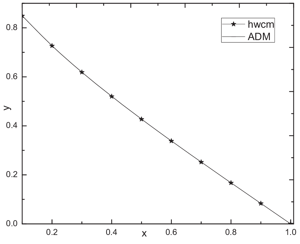
$x$	$y_{h}~(J=2)$	$y_{h}~(J=3)$	ADM [54]
0.1	0.84976	0.84909	0.84950
0.3	0.61829	0.61888	0.61937
0.5	0.42672	0.42723	0.42765
0.7	0.25187	0.25220	0.25249
0.9	0.08351	0.08361	0.08374

Problem 5.3.

Consider the problem (1.1) with BCs. (1.2) where $p(x)=q(x)=x^{0.5}$ and $f(x,y)=4x^{2}e^{y}\big(4x^{4}e^{y}-3.5\big)$ as in [55, 31, 56]. The exact solution is

y(x)=\ln\bigg(\frac{1}{4+x^{4}}\bigg).

Here, $\alpha_{1}=\ln\frac{1}{4}$ and $\beta_{1}=\ln\frac{1}{5}$ . By fixing $J=3$ with $n=7$ iterations, we obtain Haar solution $y_{h}$ . In Table 3, the numerical results of Haar solution $y_{h}$ with those the exact $y$ and ADMG solution [31] and the absolute error $e_{a}$ are shown. The graphs of the exact $y$ and hwcm solutions are plotted in Fig. 3.

Table 3: Numerical solutions and the absolute error

e_{a}

of problem 5.3

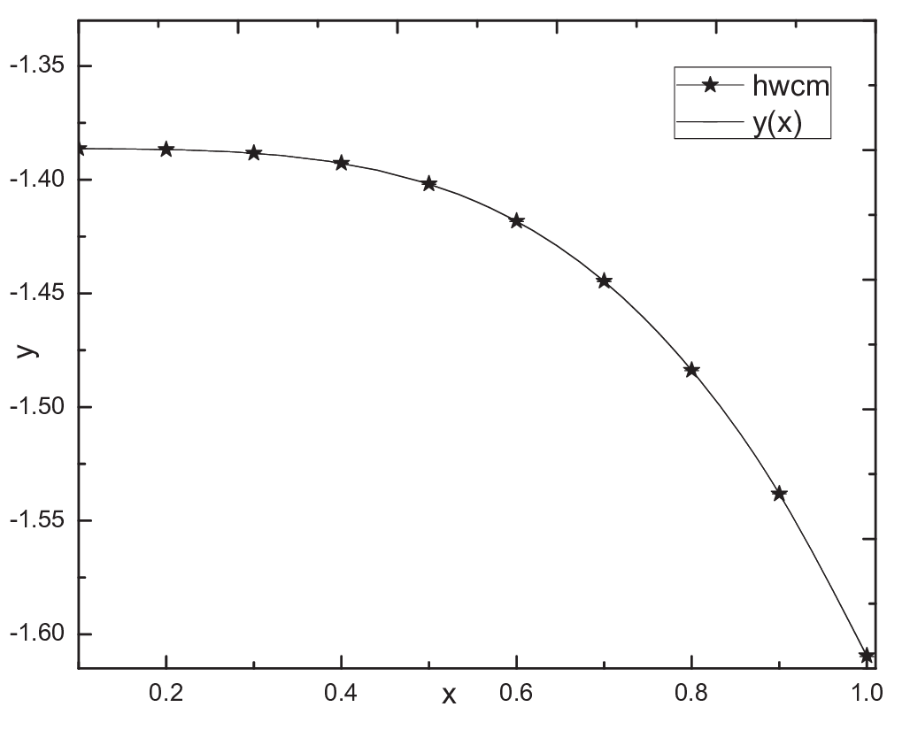
$x$	$y_{h}$	$y$	ADMG [31]	$e_{a}$
0.1	-1.38630	-1.38640	-1.38632	5.92E-05
0.3	-1.38830	-1.38840	-1.38832	6.90E-05
0.5	-1.40180	-1.40200	-1.40180	1.57E-04
0.7	-1.44460	-1.44480	-1.44459	2.22E-04
0.9	-1.53820	-1.53820	-1.53818	6.86E-05

Problem 5.4.

Consider the problem (1.1) with BCs. (1.3) where $p(x)=q(x)=x^{2}$ and $f(x,y)=y^{5}$ which describes the equilibrium of isothermal gas spheres [57]. Its exact solution is

y(x)=\bigg(1+\frac{x^{2}}{3}\bigg)^{-1/2}.

Here, $\alpha_{2}=1$ , $\beta_{2}=0$ and $\gamma_{2}=(3/4)^{1/2}$ . By fixing $J=3$ with $n=6$ iterations, we obtain Haar solution $y_{h}$ . The numerical results of Haar solution $y_{h}$ with those the exact $y$ and the ADMG [32] and the absolute error $e_{a}$ are reported in Table 4. The graphs of the exact $y$ and Haar solutions are depicted Fig. 4.

Table 4: Numerical solutions and the absolute error

e_{a}

of Problem 5.4

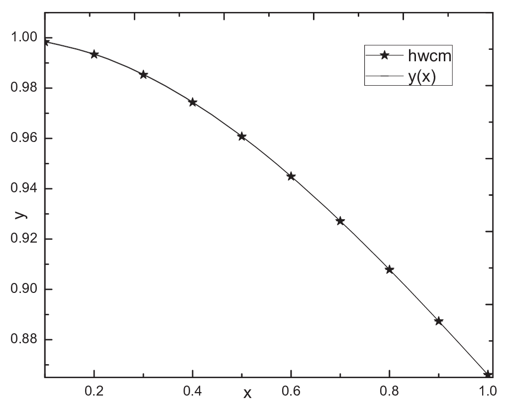
$x$	$y_{h}$	$y$	ADMG [32]	$e_{a}$
0.1	0.99834	0.99858	0.99795	2.41E-04
0.3	0.98533	0.98554	0.98501	2.11E-04
0.5	0.96077	0.96093	0.96055	1.65E-04
0.7	0.92715	0.92725	0.92703	1.04E-04
0.9	0.88736	0.88739	0.88732	3.27E-05

Problem 5.5.

Consider the problem (1.1) with BCs. (1.3) where $p(x)=q(x)=x$ and $f(x,y)=-e^{y}$ which arises an electro-hydrodynamics problem [58]. Its exact solution is

y(x)=2\ln\left(\frac{A+1}{Ax^{2}+1}\right),~A=3-2\sqrt{2}.

Here, $\alpha_{2}=1$ , $\beta_{2}=0$ and $\gamma_{2}=0$ . By fixing $J=3$ with $n=6$ iterations, we obtain Haar solution $y_{h}$ . Table 5 shows the comparison of Haar solution $y_{h}$ with those the exact $y$ and the ADMG solutions [32] and absolute error $e_{a}$ . The graphs of the exact $y$ and hwcm solutions are depicted Fig. 5.

Table 5: Numerical solutions and the absolute error

e_{a}

of Problem 5.5

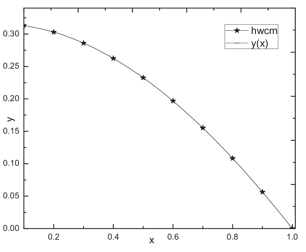
$x$	$y_{h}$	$y$	ADMG [32]	$e_{a}$
0.1	0.31327	0.31327	0.31326	8.34E-06
0.3	0.28605	0.28606	0.28604	8.08E-06
0.5	0.23270	0.23270	0.23269	7.22E-06
0.7	0.15525	0.15525	0.15525	5.41E-06
0.9	0.05643	0.05644	0.05644	2.21E-06

Problem 5.6.

Consider the problem (1.1) with BCs. (1.3) where $p(x)=q(x)=x^{2}$ and $f(x,y)=-e^{-y}$ which arises in the distribution of heat sources in the human head [10]. Here, $\alpha_{2}=2$ , $\beta_{2}=1$ and $\gamma_{2}=0$ . By fixing $J=3$ with $n=7$ iterations, we obtain Haar solution $y_{h}$ . The comparison of Haar solution $y_{h}$ with those obtained by the ADMG [32], finite difference method (FDM) [59] and the tangent chord method (TCM) [10] is presented in Table 6. The graphs of the ADMG and hwcm are depicted Fig. 6.

Table 6: Numerical solutions of Problem 5.6

$x$	$y_{h}$	ADMG [32]	TCM [10]	FDM [59]
0.1	0.26866	0.26862	0.26907	0.26875
0.3	0.25845	0.25841	0.25886	0.25853
0.5	0.23782	0.23781	0.23822	0.23791
0.7	0.20640	0.20641	0.20677	0.20649
0.9	0.16356	0.16359	0.16387	0.16365

Problem 5.7.

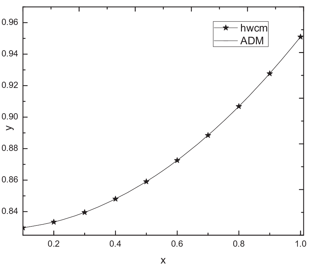
Consider the problem (1.1) with BCs. (1.3) where $p(x)=q(x)=x^{2}$ and $f(x,y)=\frac{0.76129y}{y+0.03119}$ which models a oxygen diffusion in a spherical cell with oxygen uptake kinetics [6]. Here, $\alpha_{2}=5$ , $\beta_{2}=1$ and $\gamma_{2}=5$ . By fixing $J=3$ with $n=7$ iterations, we obtain haar solution $y_{h}$ . Table 7 shows the comparison of Haar solutions $y_{h}$ with those obtained by the ADMG [32], the variational iteration method (VIM) [34] and the cubic spline method (CSM) [24]. The graphs of the ADM and hwcm solutions are depicted Fig. 7.

Table 7: Numerical results of solutions of Problem 5.7

$x$	$y_{h}$	ADMG [32]	VIM [34]	CSM [24]
0.1	0.82971	0.82970	0.82970	0.82970
0.3	0.83949	0.83949	0.83948	0.83948
0.5	0.85907	0.85906	0.85906	0.85906
0.7	0.88845	0.88844	0.88844	0.88844
0.9	0.92765	0.92765	0.92765	0.92765

Problem 5.8.

Consider the problem (1.1) with BCs. (1.3) where $p(x)=q(x)=x^{3}$ and $f(x,y)=\frac{1}{2}-\frac{1}{8y^{2}}$ which arises in the radial stress on a rotationally symmetric shallow membrane cap [60]. Here, $\alpha_{2}=1$ , $\beta_{2}=0$ and $\gamma_{2}=1$ . By fixing $J=3$ with $n=7$ iterations, we obtain haar solution $y_{h}$ . The comparison of Haar solution $y_{h}$ with those obtained by the ADMG [32] and VIM [35] are reported in Table 1. We plot the graphs of the ADM and hwcm solutions in Fig. 8.

Table 8: Numerical results of solutions of Problem 5.8

$x$	$y_{h}$	ADMG [32]	VIM [35]
0.1	0.95459	0.95458	0.95263
0.3	0.95822	0.95822	0.95649
0.5	0.96550	0.96550	0.96420
0.7	0.97648	0.97647	0.97571
0.9	0.99121	0.99120	0.99098

6 Conclusion

In this paper, the Haar wavelet quasilinearization technique has been proposed for nonlinear doubly singular boundary value problems arising in various physical models. It has been shown that Haar wavelet method with quasilinearization technique gives excellent results when applied to different physical models such as oxygen diffusion in a spherical cell [6], the heat sources in the human head [10], and shallow membrane cap [60]. The numerical results obtained by present method are better than the results obtained by other methods such as the Adomian decomposition method [31, 32], the variational iteration method [34, 35], the finite difference method [59], the cubic spline method[24] and the tangent chord method [10] and are in good agreement with exact solutions, as shown in tables 1-8 and figures 1-8 for the considered problems through 5.1-5.8. The proposed method provides a reliable technique which requires less work compared to other methods such as the finite difference and cubic spline methods. The convergence analysis of present methods have been discussed.

References

[1] L. Bobisud, Existence of solutions for nonlinear singular boundary value problems, Applicable Analysis 35 (1-4) (1990) 43–57.
[2] R. Singh, J. Kumar, G. Nelakanti, Approximate series solution of singular boundary value problems with derivative dependence using Green’s function technique, Computational and Applied Mathematics 33 (2) (2014) 451–467.
[3] R. Singh, J. Kumar, The Adomian decomposition method with Green’s function for solving nonlinear singular boundary value problems, Journal of Applied Mathematics and Computing 44 (1-2) (2014) 397–416.
[4] L. Thomas, The calculation of atomic fields, in: Mathematical Proceedings of the Cambridge Philosophical Society, Vol. 23, Cambridge Univ Press, 1927, pp. 542–548.
[5] E. Fermi, Un metodo statistico per la determinazione di alcune priorieta dell’atome, Rend. Accad. Naz. Lincei 6 (602-607) (1927) 32.
[6] S. Lin, Oxygen diffusion in a spherical cell with nonlinear oxygen uptake kinetics, Journal of Theoretical Biology 60 (2) (1976) 449–457.
[7] N. Anderson, A. Arthurs, Complementary variational principles for diffusion problems with Michaelis-Menten kinetics, Bulletin of Mathematical Biology 42 (1) (1980) 131–135.
[8] U. Flesch, The distribution of heat sources in the human head: a theoretical consideration, Journal of Theoretical Biology 54 (2) (1975) 285–287.
[9] B. Gray, The distribution of heat sources in the human head-theoretical considerations, Journal of Theoretical Biology 82 (3) (1980) 473–476.
[10] R. Duggan, A. Goodman, Pointwise bounds for a nonlinear heat conduction model of the human head, Bulletin of Mathematical Biology 48 (2) (1986) 229–236.
[11] M. Chawla, P. Shivakumar, On the existence of solutions of a class of singular nonlinear two-point boundary value problems, Journal of Computational and Applied Mathematics 19 (3) (1987) 379–388.
[12] D. Dunninger, J. Kurtz, Existence of solutions for some nonlinear singular boundary value problem, Journal of Mathematical Analysis and Applications 115 (2) (1986) 396–405.
[13] R.K. Pandey, A. K. Verma, A note on existence-uniqueness results for a class of doubly singular boundary value problems, Nonlinear Analysis: Theory, Methods & Applications 71 (7) (2009) 3477–3487.
[14] G. Reddien, Projection methods and singular two point boundary value problems, Numerische Mathematik 21 (3) (1973) 193–205.
[15] R. Russell, L. Shampine, Numerical methods for singular boundary value problems, SIAM Journal on Numerical Analysis 12 (1) (1975) 13–36.
[16] P. Jamet, On the convergence of finite-difference approximations to one-dimensional singular boundary-value problems, Numerische Mathematik 14 (4) (1970) 355–378.
[17] M. Chawla, C. Katti, Finite difference methods and their convergence for a class of singular two point boundary value problems, Numerische Mathematik 39 (3) (1982) 341–350.
[18] M. Chawla, C. Katti, A finite-difference method for a class of singular two-point boundary-value problems, IMA Journal of Numerical Analysis 4 (4) (1984) 457–466.
[19] S. Iyengar, P. Jain, Spline finite difference methods for singular two point boundary value problems, Numerische Mathematik 50 (3) (1986) 363–376.
[20] M. K. Kadalbajoo, V. Kumar, B-spline method for a class of singular two-point boundary value problems using optimal grid, Applied mathematics and computation 188 (2) (2007) 1856–1869.
[21] M. Kumar, Higher order method for singular boundary-value problems by using spline function, Applied Mathematics and Computation 192 (1) (2007) 175–179.
[22] A. R. Kanth, Y. Reddy, A numerical method for singular two point boundary value problems via chebyshev economizition, Applied Mathematics and Computation 146 (2) (2003) 691–700.
[23] A. R. Kanth, Y. Reddy, Cubic spline for a class of singular two-point boundary value problems, Applied Mathematics and Computation 170 (2) (2005) 733–740.
[24] A. Ravi Kanth, V. Bhattacharya, Cubic spline for a class of non-linear singular boundary value problems arising in physiology, Applied Mathematics and Computation 174 (1) (2006) 768–774.
[25] A. R. Kanth, Cubic spline polynomial for non-linear singular two-point boundary value problems, Applied mathematics and computation 189 (2) (2007) 2017–2022.
[26] M. Inc, M. Ergut, Y. Cherruault, A different approach for solving singular two-point boundary value problems, Kybernetes: The International Journal of Systems & Cybernetics 34 (7) (2005) 934–940.
[27] R. Mittal, R. Nigam, Solution of a class of singular boundary value problems, Numerical Algorithms 47 (2) (2008) 169–179.
[28] S. Khuri, A. Sayfy, A novel approach for the solution of a class of singular boundary value problems arising in physiology, Mathematical and Computer Modelling 52 (3) (2010) 626–636.
[29] A. Ebaid, A new analytical and numerical treatment for singular two-point boundary value problems via the Adomian decomposition method, Journal of Computational and Applied Mathematics 235 (8) (2011) 1914–1924.
[30] M. Kumar, N. Singh, Modified Adomian decomposition method and computer implementation for solving singular boundary value problems arising in various physical problems, Computers & Chemical Engineering 34 (11) (2010) 1750–1760.
[31] R. Singh, J. Kumar, G. Nelakanti, Numerical solution of singular boundary value problems using greens function and improved decomposition method, Journal of Applied Mathematics and Computing 43 (1-2) (2013) 409–425.
[32] R. Singh, J. Kumar, An efficient numerical technique for the solution of nonlinear singular boundary value problems, Computer Physics Communications 185 (4) (2014) 1282–1289.
[33] A. Wazwaz, R. Rach, Comparison of the Adomian decomposition method and the variational iteration method for solving the lane-emden equations of the first and second kinds, Kybernetes 40 (9/10) (2011) 1305–1318.
[34] A. Wazwaz, The variational iteration method for solving nonlinear singular boundary value problems arising in various physical models, Communications in Nonlinear Science and Numerical Simulation 16 (10) (2011) 3881–3886.
[35] A. Ravi Kanth, K. Aruna, He’s variational iteration method for treating nonlinear singular boundary value problems, Computers & Mathematics with Applications 60 (3) (2010) 821–829.
[36] R. Singh, N. Das, J. Kumar, The optimal modified variational iteration method for the lane-emden equations with neumann and robin boundary conditions, The European Physical Journal Plus 132 (6) (2017) 251.
[37] M. Danish, S. Kumar, S. Kumar, A note on the solution of singular boundary value problems arising in engineering and applied sciences: Use of OHAM, Computers & Chemical Engineering 36 (2012) 57–67.
[38] P. Roul, D. Biswal, A new numerical approach for solving a class of singular two-point boundary value problems, Numerical Algorithms 75 (3) (2017) 531–552.
[39] P. Roul, U. Warbhe, New approach for solving a class of singular boundary value problem arising in various physical models, Journal of Mathematical Chemistry 54 (6) (2016) 1255–1285.
[40] C.-H. Hsiao, W.-J. Wang, Haar wavelet approach to nonlinear stiff systems, Mathematics and Computers in Simulation 57 (6) (2001) 347–353.
[41] C. Hsiao, Haar wavelet approach to linear stiff systems, Mathematics and Computers in simulation 64 (5) (2004) 561–567.
[42] Ü. Lepik, Numerical solution of differential equations using Haar wavelets, Mathematics and computers in simulation 68 (2) (2005) 127–143.
[43] Ü. Lepik, Numerical solution of evolution equations by the Haar wavelet method, Applied Mathematics and Computation 185 (1) (2007) 695–704.
[44] M. ur Rehman, R. A. Khan, A numerical method for solving boundary value problems for fractional differential equations, Applied Mathematical Modelling 36 (3) (2012) 894–907.
[45] I. Singh, S. Kumar, Haar wavelet method for some nonlinear volterra integral equations of the first kind, Journal of Computational and Applied Mathematics 292 (2016) 541–552.
[46] A. Babaaghaie, K. Maleknejad, Numerical solutions of nonlinear two-dimensional partial volterra integro-differential equations by Haar wavelet, Journal of Computational and Applied Mathematics 317 (2017) 643–651.
[47] I. Aziz, B. Šarler, et al., The numerical solution of second-order boundary-value problems by collocation method with the Haar wavelets, Mathematical and Computer Modelling 52 (9) (2010) 1577–1590.
[48] I. Aziz, F. Khan, et al., A new method based on Haar wavelet for the numerical solution of two-dimensional nonlinear integral equations, Journal of Computational and Applied Mathematics 272 (2014) 70–80.
[49] R. E. Bellman, R. E. Kalaba, Quasilinearization and nonlinear boundary-value problems.
[50] R. Jiwari, A Haar wavelet quasilinearization approach for numerical simulation of burgers equation, Computer Physics Communications 183 (11) (2012) 2413–2423.
[51] H. Kaur, R. Mittal, V. Mishra, Haar wavelet approximate solutions for the generalized Lane-Emden equations arising in astrophysics, Computer Physics Communications 184 (9) (2013) 2169–2177.
[52] U. Saeed, M. ur Rehman, Haar wavelet-quasilinearization technique for fractional nonlinear differential equations, Applied Mathematics and Computation 220 (2013) 630–648.
[53] M. Inc, D. Evans, The decomposition method for solving of a class of singular two-point boundary value problems, International Journal of Computer Mathematics 80 (7) (2003) 869–882.
[54] R. Singh, J. Kumar, Solving a class of singular two-point boundary value problems using new modified decomposition method, ISRN Computational Mathematics 2013 (Article ID 262863,) (2013) 11–pages.
[55] T. Aziz, M. Kumar, A fourth-order finite-difference method based on non-uniform mesh for a class of singular two-point boundary value problems, Journal of Computational and Applied Mathematics 136 (1) (2001) 337–342.
[56] R. Singh, A.-M. Wazwaz, J. Kumar, An efficient semi-numerical technique for solving nonlinear singular boundary value problems arising in various physical models, International Journal of Computer Mathematics 93 (8) (2016) 1330–1346.
[57] M. Chawla, R. Subramanian, H. Sathi, A fourth order method for a singular two-point boundary value problem, BIT Numerical Mathematics 28 (1) (1988) 88–97.
[58] J. Keller, Electrohydrodynamics. i. the equilibrium of a charged gas in a container, Tech. rep., New York Univ., New York. Inst. of Mathematical Sciences (1955).
[59] R. Pandey, A finite difference method for a class of singular two point boundary value problems arising in physiology, International Journal of Computer Mathematics 65 (1-2) (1997) 131–140.
[60] R. Dickey, Rotationally symmetric solutions for shallow membrane caps, Quarterly of Applied Mathematics 47 (3) (1989) 571–581.

	$\displaystyle\\|y\\|$	$\displaystyle=\max_{x\in[0,1]}\|y(x)\|,~~~k_{1}=\max_{y}\|f_{yy}(y)\|,~~~m_{1}=\max_{y}\{\|f(y)\|,\|f_{y}(y)\|\}<\infty,$
	$\displaystyle g_{1}$	$\displaystyle=\max_{x\in[0,1]}\bigg\|\int\limits_{0}^{1}G(x,t)q(t)dt\bigg\|<\infty.$