TUM-HEP-1113/17
IPPP/17/87
FTUAM-17-27
IFT-UAM/CSIC-17-111
August 24, 2026
Non-resonant and electroweak NNLO correction
to the top anti-top threshold
M. Benekea, A. Maierb, T. Rauhb and P. Ruiz-Femeníac
a Physik Department T31,
James-Franck-Straße 1,
Technische Universität München,
85748 Garching, Germany
b IPPP, Department of Physics,
University of Durham,
DH1 3LE, United Kingdom
c Departamento de Física Teórica and Instituto de Física Teórica UAM-CSIC,
Universidad Autónoma de Madrid, E-28049 Madrid, Spain
Abstract
We determine the NNLO electroweak correction to the production cross section near the top-pair production threshold. The calculation includes non-resonant production of the final state as well as electroweak effects in resonant top anti-top pair production with non-relativistic resummation, and elevates the theoretical prediction to NNNLO QCD plus NNLO electroweak accuracy. We then study the impact of the new contributions on the top-pair threshold scan at a future lepton collider.
1 Introduction
The precision study of the top pair production threshold is among the main motivations for the construction of a high-energy collider [1]. About 100 fb-1 of integrated luminosity spread over ten center-of-mass energies distributed around can provide a measurement of the top-quark mass with an experimental uncertainty of about [2, 3, 4]. This must be compared to the ultimate precision possible at the LHC, which is constrained to due to the limited understanding of the relation between the mass and the mass parameter in the calculation and simulation of the final state from which the top mass is directly reconstructed. There has been some progress in the quantification of this relation when the mass is reconstructed from two-jettiness in collisions in the boosted top regime [5], but the extension of this approach to hadron collider processes requires the consideration of additional effects [6]. In addition, the top width, the strong coupling constant and the top Yukawa coupling can be extracted from the threshold scan to varying degree of accuracy.
The threshold region is defined as the kinematic regime where the top quarks have a small three-velocity of the order of the strong coupling constant . Thus, the top quarks are non-relativistic and are subject to the colour Coulomb interaction, that would facilitate the formation of toponium bound states if the top quarks were stable. The sizeable top decay width caused by the electroweak interaction also prevents hadronization. Therefore, the top threshold dynamics is governed by the colour Coulomb interaction, which must be treated non-perturbatively, while the strong coupling is still small. This interplay between the strong Coulomb attraction and the large top decay width has first been realized in [7, 8].
A significant effort has since been invested into providing high-precision predictions for top pair production near threshold. The major focus has naturally been the strong interaction effects, which have now been computed to next-to-next-to-next-to-leading order (NNNLO) accuracy [9] in an expansion where and , but . The effective field theory formalism and ingredients that underlie this calculation are summarized in [10], to which we refer for more details on the QCD aspects of the calculation.11 1 See [11, 12, 13, 14, 15, 16, 17, 18, 19, 20, 21, 22] for the computation of specific NNNLO ingredients. The NNNLO QCD result has finally settled the issue of the poor convergence of the perturbative expansion up to NNLO [23]. The NNNLO corrections are well behaved and the remaining scale uncertainty of the QCD result is at the level of . Similarly, it has been observed that the RG-improved prediction at the (almost) next-to-next-to-leading logarithmic order [24] stabilizes the scale uncertainty at the level of .
In the present work we are concerned with electroweak effects and non-resonant production of the observable final state of the decayed top anti-top pair. An analysis of various electroweak effects [25] has demonstrated that they are as large as . Thus, the full NNLO non-resonant and electroweak contributions must be included to salvage the precision of the prediction. Even more importantly, as will be discussed below, they are required to obtain a well-defined result, since the pure QCD cross section by itself contains divergences proportional to the top-quark decay width [15], which are cancelled only once the non-resonant production is included [26, 27].
The main result of this work is the NNLO calculation of all electroweak and non-resonant effects. We also provide an implementation of initial-state radiation in a scheme consistent with Coulomb resummation and the inclusion of electromagnetic corrections, following a similar treatment as for the threshold [28, 29]. To define the precise meaning of “NNLO” for electroweak effects, we note that they introduce the electromagnetic (), SU(2) electroweak () and top-quark Yukawa () coupling. For the purpose of power counting we do not distinguish between and and count
| (1.1) |
that is, an electroweak coupling counts as two powers of the strong coupling, which is consistent with counting , which is always adopted in the pure QCD calculation. The pure QCD calculation up to NNNLO then accounts for all terms in the total cross section of the form
| (1.2) |
where the global factor accounts for the phase-space suppression of the cross section near the threshold and the electroweak production in collisions. The electromagnetic, electroweak, Yukawa and non-resonant terms are of the parametric form
| (1.3) | |||||
where the first line refers to resonant and the second to non-resonant production. We note the absence of phase-space suppression and Coulomb resummation for the non-resonant part. The non-resonant contribution is known at NLO [26], but only partial results are available at NNLO [27, 30, 31]. On the resonant side, the terms arise from the QED Coulomb potential.22 2 We do not distinguish and in the other terms. These as well as all Yukawa coupling effects have already been included up to NNNLO in [25]. This result together with the NLO non-resonant and the NNNLO QCD calculation has been made available in the QQbar_threshold code [32]. The NNLO non-resonant and the remaining NNLO electroweak contributions are computed in this work, thus elevating the precision at the top-pair threshold to complete NNNLO QCD+Yukawa and NNLO EW+non-resonant. The ellipses in (1.3) denote third-order electroweak and non-resonant terms that remain unknown.
The outline of the paper is as follows. In Section 2 we describe how the calculation is split into resonant and non-resonant contributions, such that no double-counting occurs and the divergences are cancelled consistently. We also discuss the implementation of an invariant mass cut. For the practical calculation we split the total cross section into three separately finite parts, which are computed, each within its own computational scheme, in Sections 3, 4 and 5, respectively. Section 6 describes a consistency check we performed for our results and the comparison with some previous results. In Section 7 we analyze the importance of the various contributions for the threshold scan including initial-state radiation. We conclude in Section 8. Several appendices collect technical results, in particular the implementation of the new results into the QQbar_threshold code.
2 Setup of the computation
2.1 Resonant and non-resonant separation in unstable particle EFT
Precision calculations of top pair production near threshold are most conveniently done in potential non-relativistic effective field theory (PNREFT) [33, 34], which describes the dynamics of slowly moving particles with three-momentum coupled to ultrasoft radiation/massless particles with energy after hard and soft effects have been integrated out. The computation contains uncancelled divergences proportional to the top-quark width, which start at NNLO in dimensional regularization.
The top-pair production cross section is thus an ill-defined quantity. Instead one must consider the final state of the decay products . The narrow-width approximation is not applicable since the top width is not small compared to the top kinetic energy .33 3 We assume . Despite the -boson lifetime being of similar size as the top lifetime, the decay width can be dropped (expanded out) in the propagators, because the bosons are always hard. Thus, it is justified to treat the bosons as stable particles. The above final state can also be produced non-resonantly, i.e. without an intermediate non-relativistic top pair. The resonant and non-resonant production mechanisms cannot be distinguished physically and must be summed. Only the sum is well-defined and finite-width divergences must cancel [15]. This cancellation has already been demonstrated up to NNLO [27], and will be reproduced in the computation of the full NNLO correction in this paper.
To account for the non-resonant production mechanism, one must embed the effective theory framework for the QCD result [10] into Unstable Particle Effective Theory [35, 36]. The complete NNLO cross section can be written as the sum of a resonant and a non-resonant contribution
| (2.1) |
The resonant contribution has the form
| (2.2) |
It is understood that the imaginary part refers only to discontinuities of the forward amplitude that correspond to a final state.44 4 This includes cutting nearly on-shell top lines in the effective theory, since the effective top propagator contains the top width and the top is assumed to decay exclusively into . The production operators annihilate the incoming states and produce a nearly on-shell top and anti-top quark with small relative velocity. The matrix element is evaluated within PNREFT, appropriately generalized from QCD to account for electroweak effects and top decay. In addition one must consider the interactions of the energetic initial-state electrons. The are the hard matching coefficients of the production operators. They also receive electroweak corrections and furthermore acquire an imaginary part from diagrams involving cuts corresponding to and final states. The imaginary part arises, for example, from the interference of the process , where the off-shell decays to with the process , where the on-shell decays to . In unstable particle theory this contribution appears in the resonant term, since the separation into resonant and non-resonant is done strictly on the basis of the virtuality of the top propagators, which in this example is small for both and .
The non-resonant part takes the form
| (2.3) |
It originates from cuts over hard propagators that correspond to the physical final state . Hard cuts over the final state are not possible kinematically near threshold. Thus, the leading corrections are from and cuts and are of the order , which constitutes a NLO contribution to the cross section . The non-resonant term arises from expanding the full-theory diagrams in . Since both and count as two orders in the expansion, the NNLO contribution is given by the QCD corrections to the process , computed directly at the threshold , while actual cuts as well as electroweak and corrections are of the order and only contribute at NNNLO. The construction implies that the poles of internal top propagators in the non-resonant contribution are not regulated by a finite-width prescription, since any width terms would have to be expanded out. This leads to singularities at phase-space boundaries , which must be regulated dimensionally. The poles cancel exactly the finite-width divergences that appear in the resonant contribution. The computation of the QCD correction to the process with this specific prescription, required for consistency with the resonant PNREFT calculation in dimensional regularization, is the major result of the present work.
2.2 Organization of the computation
We now discuss the structure of the phase-space endpoint divergences in more detail. The clarification of their diagrammatic origin allows us to divide the sum of resonant and non-resonant NNLO contributions into several separately divergence-free parts, and this separation determines the organization of the actual calculation. The cross sections of the processes and are equal by CP symmetry, hence we shall only consider the final state below and multiply the result by two in the end.
In unitary gauge the NLO non-resonant contribution is given by the diagrams shown in Figure 1 [26]. At NNLO real and virtual gluon corrections must be considered. While this appears to be a standard NLO QCD correction computation to a process, existing automation tools can nevertheless not be employed due to the endpoint divergences, which are present in addition to the usual UV and IR singularities.
To illustrate this issue, we consider the phase-space integral of a virtual diagram such as below, where the integrand is a Lorentz scalar, i.e. it only depends on scalar products of its arguments. This allows us to define
| (2.4) | |||||
where
| (2.5) |
is the -dimensional Lorentz-invariant phase space for the process and . The Heaviside function accounts for the optional cut on the invariant mass of the top quark as will be discussed in Section 2.3. Since the bottom quark mass can be safely neglected for this calculation, for the total cross section . The real corrections can be brought into the same form as (2.4) with the variable instead of .
The endpoint divergences originate from the region , where the integrand becomes singular due to negative powers of , which stem from top-quark propagators becoming resonant. In [27] the leading terms in an expansion around of the integrands were obtained using the expansion by regions approach [37, 38]. The remaining -integration for the expanded result is trivial,
| (2.6) |
The divergent integrals with are regulated dimensionally by the in the exponent, which is inherited from the dimensional phase-space integral. At NNLO endpoint-divergent integrals with are present, but only those with manifest as poles. This is related to the well-known property of dimensional regularization, that it renders some power-like divergent integrals finite for .


It is obvious from (2.6) that the integrands must not be expanded in , because it would spoil the dimensional regularization of the endpoint divergences. This implies that the loop integrals in the virtual corrections cannot be expanded in , since even the tree-level phase-space integration is divergent. Expressions for scalar one-loop integrals in general dimensions with up to four external legs were obtained recently [39], but a simpler strategy is to take the results for the endpoint divergent terms from [27] as subtractions to the complete integrand. The integrals (2.4) are decomposed as follows:
| (2.7) |
where the required coefficients of the series expansion in are available up to order from [27]. This renders the -integration on the right-hand side finite and allows us to expand the subtracted expression in the square bracket in . Thus, the integral can be performed numerically. Additionally, we require the contributions to , because the coefficients with are multiplied with a pole in (2.7).
In total the NNLO non-resonant correction requires the evaluation of the order of 100 diagrams obtained by attaching one gluon to the diagrams in Figure 1 in all possible ways. Fortunately only about 15% of those contain endpoint divergences. They have been identified in [27] and are shown in Figures 2 and 3. They are computed manually by applying the subtractions (2.7). The remaining large number of finite diagrams is computed in an automated fashion using suitably edited MadGraph code. This latter contribution will be referred to as the automated part .


The endpoint divergent diagrams are divided into two parts. The first is given by the QCD corrections to the diagram , shown in Figure 2, and is denoted as the squared contribution . It is UV and IR finite, because it includes the complete virtual, real and counterterm contributions to . The remaining endpoint divergent diagrams, shown in Figure 3, are referred to as the interference contribution . In addition to the endpoint divergences, the interference part contains UV divergences, which are cancelled by endpoint-finite counterterm contributions contained in the automated part. We disentangle the two types of divergences by performing the subtraction (2.7) and obtain
| (2.8) |
where
| (2.9) |
is endpoint-divergent but UV-finite, and
| (2.10) |
is endpoint-finite but UV-divergent. In total, this allows us to split the non-resonant contribution into the following parts
| (2.11) |
Only the first two terms contain endpoint divergences. The third term, enclosed in square brackets, is finite. The endpoint divergences cancel with the resonant contribution. Specifically, the endpoint divergence of the interference contribution is compensated by from the bare absorptive parts of the hard matching coefficients appearing in (2.2). The are given by the diagrams in the upper and middle panel of Figure 4, which have a direct correspondence to the diagrams in Figure 3. Following this observation we split the resonant contribution into two parts,
| (2.12) |
where the remainder contains various contributions described in detail in Section 3. Here, we only point out that cancels the endpoint divergence of the squared contribution. Thus, we can now split the cross section into three separately finite parts
| (2.13) |
The finiteness allows us to evaluate each of the parts , and in a different computational scheme. They will be computed in Sections 3, 4 and 5, respectively. An overview over the divergences that appear in the individual parts , and is given in Table 1. The computations are performed in the top-quark mass pole scheme. The results are then converted to an IR renormalon-free mass scheme for the numerical evaluations performed in Section 7. The bottom-quark mass is neglected in all contributions except , where the default value GeV of MadGraph is used unless indicated otherwise.
| UV finite | IR finite | EP finite | |||
| (I) | ✓ | ✓ | ✓ | ||
| ✓ | ✓ | – | |||
| ✓ | – | – | |||
| ✓ | – | ||||
| ✓ | ✓ | – | |||
| ✓ | ✓ | – | |||
| ✓ | ✓ | – | |||
| ✓ | ✓ | ✓ | |||
| ✓ | ✓ | ✓ | |||
| ✓ | ✓ | – | |||
| ✓ | ✓ | ✓ | |||
| ✓ | ✓ | – | |||
| ✓ | ✓ | ✓ | |||
| (II) | ✓ | ✓ | ✓ | ||
| ✓ | ✓ | – | |||
| ✓ | ✓ | – | |||
| (III) | ✓ | ✓ | ✓ | ||
| – | ✓ | ✓ | |||
| – | ✓ | ✓ | |||
2.3 Implementation of a “top invariant mass cut”
The main result of this work is the non-resonant NNLO correction to the full cross section , but we also present results with loose cuts on the invariant mass of the top and anti-top quark
| (2.14) |
where () denotes the momentum of the (anti-) top quark. The implementation of cuts in the effective field theory framework has been discussed in [29] and depends on the scaling of the cut parameter with respect to the power counting parameters of the EFT. The cut is termed “loose” when . Thus, a loose cut never affects the resonant contribution to the cross section, where the off-shellness of the tops is parametrically of order .
Since the physical final state is without reference to whether it was produced through an intermediate top or anti-top, it is necessary to define what is meant by the (anti-) top momentum. An invariant mass cut of the form (2.14) was already implemented in the NLO non-resonant calculation [26], but since at this order the partonic final state is always , one simply defines , . At NNLO the final state may contain an additional gluon and a definition of the observable is required at the hadronic and the partonic level. Any sensible definition of an observable called “top momentum” should be equal up to an amount of order to the momentum of the top quark in the hypothetical limit that the top quark were a stable particle. It should also lend itself to simple, infrared-finite theoretical computations. On the other hand, the assignment of top momentum to the final state of a non-resonantly produced event is rather arbitrary and a matter of definition subject to the previous two requirements. Because non-resonant production is a sub-leading effect, different definitions differ only by small amounts.
In the following we describe an algorithm that satisfies these requirements. The algorithm is most likely not optimal and serves only as a proof of concept. In the first step we cluster any hadronic or partonic event into the objects , , -jet, -jet and other jets. For the purpose of this discussion energetic leptons and photons are also among the “other jets”. We require that the event contains exactly one , one and at least one - and one -jet.55 5 We assume here that the charges of the bosons and bottom jets have been reconstructed. In practice, this will be inefficient although a Monte Carlo study for the top forward-backward asymmetry at the ILC concluded that the discrimination between bottom and anti-bottom jets can be achieved with a purity of 80% at about 60% efficiency [40]. We also do not discuss the non-trivial combinatorial problem of reconstructing the bosons from their hadronic decay in the presence of additional jets, since in the logic of our discussion the bosons are considered as stable particles. Any jet algorithm can be used to define these objects. In a second step we group the above pre-defined objects into exactly two clusters. The momenta of these two clusters define the (anti-) top momentum. This fulfills the above-mentioned requirement, since close to threshold in an event with a resonant top and anti-top, the momentum of any other particle can be at most of order .
To implement the second step, assume that the event contains other jets and let be the set of jet momenta. A partitioning of consists of two disjoint sets , such that . The momentum of the “top cluster” and the “anti-top” cluster for a given partitioning are defined as
| (2.15) |
If there is more than one -jet (-jet) in the event, () refers to the most energetic -jet (-jet), and the remaining ones are considered to be part of the set . We then define and by the value of and , respectively, of the partitioning , which minimizes the product
| (2.16) |
An event passes the cut (2.14), if the so-defined top momenta satisfy the inequality (2.14).
We now apply this definition to the partonic NNLO calculation. The partonic final states are only at LO, and , at NLO, and at NNLO the previous and , . Here () means a final state that can originate from on-shell (anti-) top decay at the given order, with invariant mass within by an amount of order . Consider first the final state. One might think that the () decay products are automatically clustered into the correct parent () and hence the event always passes the loose cut as desired. However, this is not always true, since an energetic gluon from top decay may be radiated collinear to the from anti-top decay, in which case the jet algorithm merges it into the -jet rather than the -jet. In this case the loose-cut condition (2.14) might not be satisfied, and the event is missed even though both tops were produced resonantly.66 6 If the gluon is not energetic but ultrasoft with momentum of order , the misassignment is irrelevant and the loose-cut condition remains satisfied. Since our calculation does not include the kinematics of resonant top decay, we cannot correct it for this misassignment. However, the probability for such a misassignment is at most of order
| (2.17) |
where is the half-opening angle of the -jet. The first factor represents the suppression of energetic, large-angle gluon radiation and the second the jet area on the unit sphere. The numerical estimate is obtained for . We can therefore safely neglect this error.
Next we consider the non-resonant final state . (With obvious modifications the following discussion applies to the CP-conjugate final state.) To NNLO accuracy, on-shell top decay must be taken in NLO, and may contain an additional gluon. Whenever there is no gluon or the gluon is merged with the - or -jet, the set of partitionings is empty and the definition of and is the sum of the appropriate and -jet momenta. The loose cut is passed except when the gluon is misassigned to the -jet as above, but in this case the probability for this to occur is even further suppressed due to the suppression of non-resonant production in the first place. If, on the other hand, the jet algorithm returns an additional (gluon) jet, there are two partitionings, one where the gluon jet momentum is (correctly) added to the top decay, i.e. to , and the other, where it is not. The first, correct, possibility will almost always minimize in (2.16) and then satisfy the loose-cut condition, whenever the invariant mass of the non-resonant pair is larger than , where . Hence, imposing the cut yields a single Heaviside function in the phase-space integral, as in (2.4). The other partitioning where the additional gluon jet is incorrectly combined with the non-resonant to form the anti-top momentum can minimize only if the invariant mass of the , -jet and gluon jet accidentally adds up to within an amount . This possibility is suppressed by the NNLO probability for the process to happen in the first place times the small phase-space fraction where the kinematic requirements for misassignment are satisfied, and hence can be neglected at NNLO.
Finally we discuss the final state, which appears at NNLO in the non-resonant part. At NNLO, it is sufficient to consider the resonant top quark decay in the tree approximation. Hence, the discussion of the final state from above can be repeated, except that now the partitioning that minimizes with overwhelming probability is the correct combination of the gluon jet momentum with the non-resonant pair. Hence, up to a negligible error, the loose cut (2.14) is implemented in the real-emission phase-space of the NNLO non-resonant contribution as the Heaviside function .
We have not implemented other cuts, but it is in principle straightforward to do so as long as they are loose. A general cut is a function of the external momenta, which evaluates to one if the event passes the cut and to zero otherwise. We define the complementary cut as . Assuming that is loose, the complementary-cut cross section is purely non-resonant and free of endpoint divergences. It can therefore be computed with automated NLO parton level event generators such as MadGraph [41]. The non-resonant contribution with the original cut is then given by subtracting from the total cross section, where the cancellation of divergences between the resonant and non-resonant parts has already been taken care of. This approach will also be exploited in Section 6.1 to perform a powerful check of our computation.
A generalization to arbitrary cuts would affect the resonant contributions and is beyond the scope of this work. Recently, first results of an implementation of the fully differential cross section with NLL accuracy near threshold matched to the NLO fixed order result have been presented [42], but the generalization of this method to NNLO accuracy as discussed here is not straightforward.
3 Part (I)
The scheme for part (I) as defined in (2.13) is fixed by the existing QCD results for . The resonant QCD cross section factorizes into a leptonic tensor and the correlation function of two top-quark currents, . The former is evaluated in four dimensions; the latter completely in dimensions in the naive dimensional regularization scheme (NDR). The squared contribution contained in part (I) factorizes into the same leptonic tensor and a hadronic tensor , and the same conventions must be applied. We compute this part in Section 3.2. The electroweak NNLO corrections to the resonant part must also abide by this scheme (except for contained in part (II)), and we consider them first.
3.1 Resonant electroweak effects
Electroweak corrections to the resonant cross section are computed in the non-relativistic EFT framework extended from QCD to the full Standard Model. We consider them to NNLO in the counting scheme (1.1).
For ease of reference and to set up notation, we briefly recapitulate the well-known expressions for the LO cross section [32]
| (3.1) |
where is the high-energy limit of the photon-mediated muon pair production cross section at leading order, and is the on-shell top-quark width as defined below. At LO the top pair is produced via s-channel exchange of a photon or boson. The couplings of the fermions to the boson are given by
| (3.2) |
where is the third component of the weak isospin of fermion , is the fermion electric charge measured in units of the positron charge, and and are the sine and cosine of the Weinberg angle, respectively. The S- and P-wave production operators are given by77 7 Note and is summed from 1 to 3.
| (3.3) | |||||
| (3.4) | |||||
| (3.5) | |||||
| (3.6) |
with leading-order matching coefficients
| (3.7) | |||
| (3.8) |
Here is the non-relativistic top (anti-top) field and denotes the effective field (as defined in soft-collinear effective theory (SCET)) of an energetic electron moving in the light-like direction . In the present context, the directions and are set by the electron and positron beams, respectively. The collinear electromagnetic Wilson lines
| (3.9) |
have been introduced to make the operators invariant under collinear gauge transformations in SCET, as well as the light-like vectors with . The factor of has been absorbed into the operators to render the coefficients dimensionless and of order one. The P-wave production operators and their Wilson coefficients will be required below. Note that because the cross section is constructed as an expansion in , the energy-dependence of the -channel photon and boson propagators could be expanded around , in which case the short-distance matching coefficients would be truly energy-independent. However, we apply a convention where we keep the full -dependence in the -channel propagators, which therefore appears in (3.3) to (3.8).
The renormalization scheme for the electroweak parameters adopted here is the scheme. The Weinberg angle is then given by (). The electromagnetic coupling from now on is denoted by , where refers to the scale dependent electromagnetic coupling defined through the photon vacuum polarization, which interpolates between the fine-structure constant and the input parameter .
In (3.1) denotes the non-relativistic zero-distance Coulomb Green function in dimensional regularization [43, 44],
| (3.10) |
which describes the propagation of the top-anti-top pair at LO in the non-relativistic EFT. It is expressed through the variable
| (3.11) |
and , where is the logarithmic derivative of the gamma function. Furthermore, the logarithm appears.88 8 When the pole is related to a finite-width divergence, we set and write and to distinguish the finite-width scale-dependence of the resonant contribution from the scale-dependence due to the strong coupling, cf. [22, 14].
After separating from the NNLO resonant contributions as explained around (2.12), the remaining parts are
| (3.12) |
The pure QCD S-wave contribution has been obtained in the formalism employed here in [34]. Top-pair production in a P-wave state was computed in [22]. Higgs contributions that only involve the top Yukawa coupling have been computed already up to NNNLO [25, 45]; similarly the effect of the LO QED Coulomb potential [25]. At NNLO, top decay introduces additional contributions to the bilinear part of the PNREFT Lagrangian, which contribute to the resonant cross section (Section 3.1.1). While there are no electroweak contributions to the non-relativistic potential at NNLO (Section 3.1.2), there are electroweak corrections to the hard matching coefficients . The contribution from the real part of the hard matching coefficients is given in Section 3.1.4. Contrary to the QCD case the electroweak hard matching coefficients contain an imaginary part from cuts over all possible final states. The () cuts contribute to the cross section [46]. The imaginary part is split into a bare contribution (Section 4.1) and a contribution from field renormalization (Section 3.1.3), because the two parts are treated in different schemes. Partial results for the mixed-QCD-electroweak corrections to the hard matching coefficients are available [45, 47], but they only contribute at NNNLO and will not be considered here. Finally, we consider effects from initial-state radiation (ISR), (Section 3.1.5).
3.1.1 Finite-width corrections to the NNLO Green function,
Additional terms appear in the PNREFT Lagrangian due to the instability of the top quark and its coupling to photons. The coupling of the top quarks to ultrasoft photons must be multipole expanded in the spatial component, just like the interactions with the ultrasoft gluons. Only the leading term
| (3.13) |
is relevant at NNLO. However, its contribution vanishes, because the multipole-expanded field can only resolve the net electric charge of the top anti-top pair, which is zero. In analogy to QCD, the couplings in the Lagrangian (3.13) can be removed by a field transformation involving an ultrasoft Wilson line (cf. [48]). The generalization of the bilinear part of the PNREFT Lagrangian is [35, 36]
| (3.14) | |||||
where is the non-relativistic top (anti-top) field and is a hard matching coefficient. It can be determined by matching the top propagator in the effective theory to the full theory. In the pole mass scheme we obtain
| (3.15) |
where is the pole width of the top quark defined through the gauge-invariant position of the pole of the top propagator
| (3.16) |
in the complex plane. We note that with this convention (3.14) contains the term , which has the form of a mass shift. It can be absorbed into the definition of the pole scheme by adding to the right hand side of (3.16), which completes the square and defines a different convention used e.g. in [49]. Electroweak corrections to the top-pair production cross section near threshold have also been considered in [50]. The absence of the correction to the Green function in [50] implies that this different convention is also adopted there. Thus, one must be careful to account for this difference in the definition of the top pole mass when comparing their results to ours.
The term in (3.14) belongs to the LO Lagrangian and must be treated non-perturbatively. It leads to the replacement , which defines the QCD contribution, and makes the argument of the Green function in (3.1) complex. The two remaining terms in (3.14) that contain the width are of NNLO and can be treated perturbatively. Only two simple single insertions are required. We denote the correction to the Green function from the terms and by and , respectively. They are given by
| (3.17) | |||||
| (3.18) | |||||
where is the first derivative of the polygamma function. The corresponding NNLO contribution to the Green function is
| (3.19) |
In the implementation of the cross section in the QQbar_threshold code [32] the top width is treated as a parameter. This implies that higher-order corrections to the tree-level width are also treated non-perturbatively through the replacement . A subtlety arises at electroweak NNLO when this result is combined with the non-resonant contribution, which is computed in dimensional regularization. The pole part of the NNLO non-resonant contribution is proportional to with a finite part that follows from expanding diagrams up to . For consistency, the tree-level contribution to the width in (3.14) must be treated as a -dimensional hard matching coefficient. Hence the terms in the -dimensional tree-level expression of the top width contribute finite terms to the resonant part from their multiplication with the finite-width poles. These finite parts are not included when is treated as a four-dimensional numerical parameter, and must be added separately.99 9 QCD corrections to the width, however, are only needed in four dimensions where they are known up to NNLO [51, 52].
The LO pole width, which is required in dimensions, is given by
| (3.20) |
where and denotes the scale related to the finite-width divergences as discussed in [22, 14]. The contribution from the terms of (3.20), which multiply the finite-width divergence contained in (3.19) and the one in the pure QCD result, to be added to the cross section is
| (3.21) | |||||
where is the limit of (3.20). On the whole, we obtain
| (3.22) |
In the numerical evaluation we resum the perturbative corrections to the would-be toponium bound-state poles. Due to the instability of the top quarks, we are dealing with a non-Hermitian Lagrangian, cf. (3.14). The implications have been discussed in [53]. The positions of the would-be toponium poles are the complex eigenvalues
| (3.23) |
of the non-Hermitian Hamiltonian, where is the bound-state energy assuming stable top quarks and is the total inclusive width of the bound state. In accordance with the earlier discussion, the top-quark width is treated as a parameter. The corrections describe the effects of time dilatation on the top decays due to the residual movement of the top quarks and the annihilation of the would-be toponium state through strong (e.g. ) or electroweak (e.g. ) interactions.
The eigenstates of a non-Hermitian operator do not form an orthogonal basis of the Hilbert space [53]. This implies, that the completeness relation must be modified. We consider the sets of right and left eigenstates1010 10 We do not distinguish between bound states and continuum states, since this is irrelevant for the discussion.
| (3.24) |
with . Assuming that the Hamiltonian transforms as
| (3.25) |
under time reversal, and that the eigenvalues are non-degenerate, the eigenstates can be normalized such that they form a bi-orthogonal set [53]
| (3.26) |
which implies that the completeness relation takes the form
| (3.27) |
The property (3.25) implies that the state is exponentially growing at the same rate as is decaying, which facilitates the normalization (3.26). After applying (3.27) the Green function takes the following form near the poles
| (3.28) |
which generalizes the expression for the QCD result [14]. The pole position and residue of (3.28) have the following perturbative expansion
| (3.29) | |||||
| (3.30) |
with the LO expressions
| (3.31) | |||||
| (3.32) |
and . At LO we have made use of the relation . This holds, because the non-Hermitian part of the LO Hamiltonian
| (3.33) |
is proportional to the identity operator and thus only affects the eigenvalues but not the eigenstates .
The results for the non-relativistic Green function in perturbation theory do not take the form (3.28), but contain higher-order poles
| (3.34) | |||||
This allows us to read off the NNLO correction to the bound state parameters from the contribution (3.19) to the Green function
| (3.35) | |||||
| (3.36) | |||||
| (3.37) |
As discussed above, the term in (3.14) has the form of a mass shift and therefore leads to an -independent correction (3.35) to the position of the pole, while it does not affect the residue. The term in (3.14) accounts for time dilatation, which reduces the total width of the would-be toponium resonance by (3.36). Since it is non-Hermitian, it also makes the residues complex due to (3.37).
The corrections to the bound states from QCD effects as well as the QED Coulomb and Higgs potentials can be found in [14] and [25], respectively. Using this input we can resum the higher-order poles in the expanded Green function by the replacement
| (3.38) |
where the expanded term has the form (3.34). In the actual implementation [32] we apply the pole resummation procedure to alone in the electroweak contributions, but to the entire current correlation function of vector and axial vector currents in the pure QCD contributions.
3.1.2 Mixed QCD-electroweak NNLO corrections in PNREFT
In addition to the kinetic terms (3.14) the PNREFT Lagrangian contains potential interactions. We now show that there are no mixed QCD-electroweak corrections at NNLO. The construction of PNREFT proceeds by first integrating out fluctuations at the hard scale, which yields NREFT, and then integrating out fluctuations at the soft scale. In the first step, one must consider electroweak corrections to the hard matching coefficients of the QCD vertex, and vice versa. The relevant diagrams are shown in Figure 5. The loop momenta in Figure 5 are hard, while the momenta of the external particles can be either soft, potential or ultrasoft and must be expanded out of the loop integral. Therefore the vertices are effectively evaluated at zero external momentum, and the corresponding contribution is exactly cancelled by the on-shell external field renormalization factor.

The potentials are determined in the matching procedure between NREFT and PNREFT. The diagrams that contribute to the potential at order are shown in Figure 6, where the momenta of the external top quarks are potential and the loop momentum is soft. The contributions of the first and second diagram are identical, and are exactly opposite to those of the third and fourth diagram, which implies that the sum of the diagrams in Figure 6 vanishes. We have not drawn the four diagrams that involve soft vertex corrections to the tree-level potentials, because these corrections are scaleless and vanish in dimensional regularization. Last, but not least there are no contributions from insertions of the one-loop corrections to the hard matching coefficients in the tree-level potential, because these coefficients vanish as argued above. We conclude that no mixed QCD-electroweak potentials appear at NNLO.

Furthermore, we demonstrate that the potential does not receive any pure electroweak NNLO corrections from the exchange of Z bosons. We count the mass of the Z bosons as hard and therefore have to integrate out the Z boson in the hard matching to NREFT. This implies, that all interactions that are mediated by the Z boson in the full theory become local in PNREFT. The Z-boson exchange potential corresponds to the full-theory diagrams shown in Figure 7 and is proportional to in momentum space. Thus, it is suppressed by compared to the LO colour Coulomb potential and only contributes at NNNLO.

Finally, we comment on the so-called ‘jet-jet’ interactions that were considered in [54]. These are corrections involving gluon emission from the final-state bottom quarks and it was demonstrated in [54] that they vanish at NLO. In their calculation, the authors of [54] first consider the subgraph , which corresponds to the cut to the right of the gluon of the third diagram in Figure 5. Their result for scales as , where is the gluon three-momentum, which is either potential or ultrasoft in their case. They then show by explicit computation that all NLO corrections that involve the subgraph and/or its CP conjugate vanish. In our approach, where loop integrals are strictly expanded according to the scaling of the momentum regions, the only non-vanishing contribution to the subgraph comes from the region of hard loop momentum, where no inverse powers of can appear because the external momenta are expanded out. Therefore, the absence of any ‘jet-jet’ interactions at NLO is a matter of simple power counting, which implies that corrections can first appear at the relative order , i.e. at NNLO. We have already proven that there are also no ‘jet-jet’ interactions at NNLO by demonstrating that electroweak corrections to the QCD vertex in Figure 5 vanish.
3.1.3 Absorptive part from field renormalization,
The hard matching coefficients become complex at NNLO due to loop corrections. The imaginary part contributes to the finite-width divergence of the resonant cross section in (3.12) and, thus, it has to be determined in dimensions in accordance with the scheme used to evaluate the other components of part (I). The bare absorptive contribution to on the other hand, is contained in part (II) and therefore has to be computed in a different scheme. Since the two parts are treated using different conventions, we find it convenient to separate them in notation. The matching coefficients up to NNLO are expanded as
| (3.39) |
| (3.40) |
The real part of the electroweak corrections, , does not yield a finite-width divergence at NNLO. Thus, it is not necessary to split it as well. The absorptive part (3.40) of the hard matching coefficient is available in four dimensions [46]. We have repeated the calculation of the individual contributions in the schemes described above. In four dimensions we reproduce the result of [46],
| (3.41) |
where the normalization factor is necessary because the definition of the hard matching coefficients in [46] differs from (3.39).
The bare part will be given in Section 4.1. From the field renormalization, we obtain
| (3.42) | |||||
| (3.43) | |||||
The contribution to the NNLO cross section is given by
| (3.44) |
where the finite terms from the multiplication of the divergence in the real part of the Green function (3.10) with the parts of (3.42) and (3.43) are included.
3.1.4 Electroweak contributions to the hard matching coefficient,
The real part of the electroweak contributions to the NNLO matching coefficients has been computed in [55, 56, 57]. Pure QED corrections have been neglected there. Therefore, we split
| (3.45) |
The hard QED vertex correction to the and vertices contains divergences that cancel among initial-state radiation (ISR) contributions (see Section 3.1.5). We therefore assign it to to render both, and , separately finite. There is no contribution from the box diagram involving two photons, since only its interference with the production of the top pair through the vector component of the -channel or boson is of NNLO and the correlator of three vector currents vanishes [58]. The box diagram with a photon and boson is considered to be a non-QED correction to the photon-exchange contribution and is therefore already part of . Thus, the only pure QED effects are the hard photon vertex correction to the and currents and the photon self energy, which yield
| (3.46) |
As in [59], the renormalized photon self-energy is defined in the scheme of [60], and will be discussed below. The non-QED contributions are
| (3.47) |
where is given in [57], is the fine-structure constant and coincides with the expression for from [57]. The subtraction terms are present because Higgs effects which only involve the top Yukawa coupling have already been included separately as part of in [25] and the photon self-energy is contained in the QED contribution (3.46). Corrections that involve Higgs couplings to gauge bosons or Goldstone bosons remain in (3.47).
We note that the photon self-energy terms in (3.46) and (3.47) differ, because we use a renormalization scheme which is different from [55, 56, 57]. The matching coefficients given in [55, 56, 57] are expressed in terms of the fine-structure constant . This scheme suffers from a large spurious dependence on the light fermion masses, that cancels explicitly with the self-energy corrections to the matching coefficients when the fine-structure constant is expressed in terms of a less infrared-dependent definition of the electroweak coupling constant. Therefore, we write the cross section in terms of the running on-shell coupling from [60]. In this scheme the renormalized photon self-energy takes the form
| (3.48) |
where the bare self energy is taken from [55]. The explicit factor appears, because [55] defines the photon vacuum polarization as a dimensionful quantity and does not imply a power-dependence of the cross section on the scale . In the limits and the scheme of [60] converges to the scheme of [55, 56, 57], i.e. and , and the self-energy terms in (3.46) and (3.47) coincide with each other and with the respective expression in [57].
The cross section receives the contribution
| (3.49) |
from the electroweak corrections to the hard matching coefficients of the production operators.
3.1.5 Initial-state radiation,
In this section we take into account effects from QED initial-state radiation. As such we count all corrections that involve an additional photon attached only to the external states relative to the LO cross section. ISR was already considered in the 1980s [8] at the leading logarithmic order, i.e. summing corrections of the form to all orders, whereas later works concentrated on the ‘partonic’ cross section. We extend the treatment of ISR to NNLOLL accuracy below. The non-resonant part is only affected by QED radiation at NNNLO and will not be considered. With the exception of the effects from the hard momentum region, all contributions are universal and our treatment closely follows the one for pair production near threshold in [28, 29]. In fact, the equations in this section can often be obtained directly from those in [29] by substituting , and by adapting the different tree-level process.1111 11 Compared to our results the expressions in [28, 29] contain an extra factor from the -dimensional spin sum over the initial state which we treat in dimensions as described at the beginning of Section 3.
When the electron mass is neglected the ISR contribution involves the hard, , and ultrasoft, , momentum regions, and in addition two hard-collinear momentum regions, () familiar from SCET, where are pairs of light-like vectors with defined by the electron () and positron () momentum. Real collinear emission is kinematically forbidden in the resonant part, because it carries away a hard momentum fraction, which pushes the top pair off-shell. Virtual collinear corrections are scaleless. Hence, the hard-collinear regions vanish [28], and we are left with the hard and ultrasoft contributions. We evaluate these separately. A hard photon cannot be exchanged between the incoming and outgoing electrons, since this would also push the top pair off-shell. Thus the only correction from the hard region is the QED vertex correction which contributes to the hard matching coefficients . We find
| (3.50) | |||||
As it should be, this agrees with the QCD analogue of the hard matching coefficient of the vector current to SCET, first obtained in this context in [61] in DIS kinematics. We only kept the real part, because the imaginary part comes from cuts that do not correspond to the final state . The correction to the cross section from hard ISR is
| (3.51) |
The contributions from the ultrasoft momentum region are shown in Figure 8. Virtual ultrasoft corrections are scaleless. The diagram with the photon attached to incoming and outgoing electron vanishes, because it is proportional to the square of the light-like direction of the electron beam.

No ultrasoft corrections that couple to the collinear and non-relativistic sector occur at NNLO, because the leading ultrasoft photon coupling to the final state vanishes, as discussed in Section 3.1.1. Thus, the contribution to the cross section from the ultrasoft region is due to the right diagram in Figure 8 and reads
| (3.52) |
When the small electron mass is neglected, the photon radiation corrections are given by the sum of (3.51) and (3.52). We observe that the pole cancels, but a collinear divergence remains, because the cross section is not infrared safe for . Subtracting this divergence defines a scheme-dependent ‘partonic’ cross section.
The divergence is regularized by the non-zero electron mass, which in turn yields large logarithms . They can be resummed into an electron distribution function , which describes the probability of finding an electron with momentum in the “parent electron” with momentum . The cross section with resummed ISR from the electron and positron is given by
| (3.53) |
Expressions for the structure function at leading-logarithmic (LL) accuracy can be found in [62, 63, 64, 65], where LL implies that all terms of the form are summed to all orders. The resummation of the next-to-leading logarithms (NLL) is crucial for the precision program at a future lepton collider, but the structure functions are presently unknown at this order.
At LO, the ‘partonic’ cross section is given by (3.1). At higher orders it depends on the scheme used to regularize and subtract the collinear divergence. The scheme dependence cancels in the convolution with the structure functions. This implies that we have to adapt the results (3.51) and (3.52), which correspond to a minimal subtraction scheme, to the conventional scheme in which the structure functions are defined. This procedure has been described in detail in [28, 29]. First, we need to convert the dimensional regulator of the collinear divergences to a finite electron mass regulator. Then, the terms that appear in the convolution of the structure functions with the LO cross section have to be subtracted from the fixed order NNLO partonic cross section to avoid double counting.
The first point is accomplished by noting that the presence of the additional scale introduces the additional momentum regions
| (3.54) |
with and , respectively. The soft-collinear region contributes in the diagrams shown in Figure 8. As before, the left diagram vanishes, and one finds
| (3.55) |
The hard-collinear contribution comes from vertex correction diagram and gives
| (3.56) | |||||
The collinear poles cancel in the sum of the hard and hard-collinear, and ultrasoft and soft-collinear contributions, separately. The collinear sensitivity is instead expressed through the large logarithms . The remaining singularities cancel in the sum over all regions. To make the cancellation explicit, one can expand the factor in the distribution sense:
| (3.57) |
where is arbitrary and we have introduced the modified plus-distribution
| (3.58) |
We obtain
| (3.59) | |||||
which is finite, such that the four-dimensional expression (3.10) for the LO Green function can be used. The -dependence cancels.
We determine the subtraction terms by expanding the convolution of the LO cross section with the structure function in the coupling constant. We take the expression for the electron structure function from [65] with , given by
| (3.60) | |||||
The perturbative expansion of the structure function can be written as
| (3.61) |
For the determination of the subtraction term only the limit is important,
| (3.62) |
The term in the convolution of the leading order partonic cross section with the structure functions is
| (3.63) | |||||
where in the non-relativistic Green function was evaluated at and we have substituted . We also set and neglected the difference between and in the argument of the logarithm. The initial-state QED correction to the partonic cross section in the conventional scheme for the electron structure function is given by (3.59) with (3.63) subtracted, resulting in
| (3.64) | |||||
The imaginary part of the Green function is neglected for outside the non-relativistic regime. The photon radiation contribution (3.64) to the cross section in this scheme is finite and free of large logarithms of the electron mass.
3.2 The squared contribution
In this section we discuss the calculation of the squared contribution in (2.13), which is given by the diagrams in Figure 2. The computer programs Package-X [66], FeynCalc [67, 68] and LoopTools [69] have been employed for certain steps of the computation. The result for the scalar four-point integral in the diagram was taken from [70]. The individual diagram contributions to the hadronic tensor are evaluated in dimensions and written in the form (2.7). The numerical (or ) integral contains all terms with positive integer or half-integer powers of . With the exception of , the subtracted integrands were all obtained in analytical form. The integrand for contains an additional numerical angular integral. The expressions for the integrands are rather lengthy and will not be given explicitly. The numerical integrals are plagued by integrable singularities involving and terms, that cause numerical instabilities in the evaluation of some diagrams. As a remedy, we computed additional terms in the expansion in analytically and used them as further subtractions.
The contributions corresponding to the second term on the right-hand side of (2.7) are given by the sum of the respective expressions in [27] and terms from the contributions to . The latter encapsulate the dependence of the squared contribution on the computational scheme and are therefore specified below. In the notation of [27], we obtain1212 12 Note that in the expressions from [27] quoted below and in Section 4.2, in [27] must be interpreted as and in [27] must be identified with .
| (3.65) | |||||
where is the contribution from the first term on the right-hand side of (2.7). The prefactor is defined as
| (3.66) |
The other diagrams in Figure 2 do not contain poles from the endpoint divergence and, therefore, no terms of this type are present, i.e. .
The contribution of an individual diagram , to the non-resonant part is
| (3.67) |
where is a symmetry factor, that is either two for diagrams which are symmetric with respect to the cut, or four for diagrams which are not symmetric with respect to the cut. The photon couplings are and , where is the fermion charge measured in units of the positron charge, and couplings of the fermions to bosons are given by (3.2). The photon mass obviously vanishes, . In (3.67), terms in the leptonic tensor have been discarded, as discussed at the beginning of this section. We have checked explicitly that IR and UV divergences cancel in the sum over the diagrams in the squared contribution.
4 Part (II)
It would be a natural choice to use the same scheme for part (II), given by (see (2.13))
| (4.1) |
as for part (I). We can however simplify the computation of this part by performing the Dirac algebra and one of the loop integrations in four dimensions. The details of this scheme and the computation of and are shown in Section 4.1 and 4.2, respectively.
4.1 Absorptive contribution to the matching coefficient
The bare absorptive part of the matching coefficients is given by the diagrams shown in the second row of Figure 4. We define the scheme as follows: The coefficients are calculated in four dimensions, but the loop integrations in the third row of Figure 4, i.e. the ones related to the non-relativistic Green function, are performed in dimensions. The Dirac algebra is completely treated in four dimensions. We describe in Section 4.2 how the interference contribution must be treated to achieve consistency with this scheme.
Our results for in four dimensions are
| (4.2) | |||||
| (4.3) | |||||
The contribution to the cross section is given by
| (4.4) |
We recall that at LO the Dirac structure of the top anti-top pair becomes trivial in the non-relativistic regime and only yields a prefactor . By introducing the factor in front of the Green function in (4.4), we adapted the expression to the scheme described above, which involves four-dimensional Dirac algebra. The contribution (4.4) is not affected by loose cuts.
4.2 Endpoint divergence of the interference contribution
The endpoint-divergent part of the interference contribution has been computed in [27]. The expression (2.9) also contains an endpoint-finite term from the terms in multiplying the pole. This term carries the dependence on the computational scheme and must, therefore, be treated in the same scheme as the contribution (4.4). We evaluate it using the expansion by regions approach described in [27]. For each of the diagrams in Figure 3, we treat the loop contained in the corresponding diagram in Figure 4, i.e. the right loop in and the left loop in and , in four dimensions. The Dirac algebra is also done in four dimensions, but the remaining loop integrations are performed in dimensions. In the notation of [27] we obtain
| (4.5) | |||||
| (4.6) |
with for diagram with a photon attached to the vertex, and for the vertex. The endpoint divergent contributions of and follow from equation (3.67) with . The contribution of is given by
| (4.7) | |||||
with symmetry factor .
To verify that the treatment of the scheme is consistent we computed the finite sum of the contributions from the diagrams and and the contributions from the corresponding diagrams in also in the scheme of part (I) and found perfect agreement with the results presented above. Applying the scheme of part (II) simplifies the computation, especially for , since it avoids the more complicated integration of the left loop in in dimensions.
5 Part (III)
The part (III) contains the automated part , which is evaluated with MadGraph. The automated part is UV divergent and therefore scheme dependent. The divergence and the corresponding scheme dependence cancel with the endpoint-finite part of the interference contribution. We first describe the implementation of the automated part in MadGraph in Section 5.1. This fixes the scheme in which is computed in Section 5.2.
5.1 The automated part
We first recall some aspects of MadGraph, which are relevant to our definition of the computational scheme.
- 1.
The subtraction of IR singularities is performed automatically using the FKS method [71, 72]. The IR singularities in the real corrections are subtracted before the phase-space integration and the subtraction terms are then integrated over the phase space of the real emission and added to the virtual corrections, where they cancel the IR singularities that arise in the loop integrals. The phase-space integration is then always done in four dimensions.
- 2.
In the virtual corrections, MadGraph uses rational terms [73] to absorb the -dimensional parts of the numerators. For a given diagram with amplitude the decomposition takes the form
(5.1) where , quantities with a bar are -dimensional and quantities without are 4-dimensional. The non- term can be written as a sum over 4-dimensional coefficients multiplying -dimensional tensor integrals. The -dimensional parts related to the implementation of the ’t Hooft-Veltman scheme [74] in MadGraph are all contained in the terms.
- 3.
The amplitudes for the non- terms, the terms, the UV counterterms and the FKS subtraction terms are written as separate lists, each of them containing the coefficient of the pole, the pole and the finite part. Afterwards, only four-dimensional operations are performed, i.e. the multiplication with the conjugated four-dimensional born amplitude and the four-dimensional phase-space integration.
Given the way that is defined, we never have to modify the construction of an amplitude , but we have to remove certain contributions in the squared amplitude . All the contributions associated with the diagrams in Figure 2 have to be removed, i.e. also the parts, the UV counterterms and the FKS subtraction terms. There is however an ambiguity in the subtraction of the contributions in Figure 3, which determines the scheme in which must be computed. We choose to only subtract the non- terms of with . Following the discussion of the items 1 and 2 above, this implies that has to be computed by using dimensional regularization for the tensor integrals. All other steps in the computation of are then performed in four dimensions.
In the following, we describe the steps we performed in MadGraph to obtain the automated part in the scheme defined above. It is obvious that this cannot be achieved by modifying the process generation, because the automated part does not correspond to a squared amplitude. We therefore first generate the full process including QCD corrections. By not invoking the complex mass scheme, we make sure that the self-energy insertions are treated perturbatively. Hence, the cross section diverges rapidly for center-of-mass energies approaching from below. We remove the contribution from the endpoint divergent born diagram , the diagrams shown in Figures 2 and the non- terms from Figure 3 by editing the code generated by MadGraph.
Finally, we have to deactivate some checks inside the code, that are invalidated by the modifications. MadGraph checks if the and poles vanish for a number of phase space points. Here, this is not the case because the automated part is UV divergent. We have addressed this issue with in two ways – by deactivating the check or by performing a minimal subtraction of the UV divergence – and found agreement of both approaches. The minimal subtraction was also used to verify the cancellation of the UV divergence with the endpoint-finite part of the interference contribution . Furthermore, due to the subtractions, the tree-level cross section and the real corrections are no longer the squared absolute value of an amplitude and, thus, no longer positive for all phase-space points. The positivity of these expressions is not necessary to make the code run properly, but is only used as an internal check [75]. Therefore, we can safely switch it off. The code can now be evaluated directly at the threshold . The contribution is given by the difference of fixed-order runs at NLO and LO, multiplied by a factor two to account for the contributions. Further details on the implementation and modifications in MadGraph are provided in Appendix B. The evaluation of the automated part in the code QQbar_Threshold relies on a precomputed grid as described in Appendix A.5. Since the contribution is rather small, we do not aim for more precision than about 10% in the automated part. The resulting error of the cross section is less than one per mille. To reach this target precision we set up MadGraph to generate an integration grid from four iterations with 15000 points per integration channel and perform the actual integration using six iterations with 100000 points for each point of the QQbar_Threshold grid. More precise results are possible at the cost of a considerably increased computing time for the generation of the grid.
5.2 Endpoint-finite part of the interference contribution
We recall that the endpoint-finite part of the interference contribution has the form (2.10). As detailed in Section 5.1 it must be evaluated by taking only the tensor integrals of the virtual loop in dimensions and then performing all other steps in the computation strictly in four dimensions. Within this scheme, we have determined the endpoint subtracted integrands for the diagrams analytically and for as a one-dimensional angular integral. We refrain from giving the lengthy results for the integrands. As described in Section 3.2 we use additional terms in the expansion of the amplitudes in as subtractions to deal with integrable divergences that appear in the limit of the -integration. The result for is given by applying the same prefactors and symmetry factors as for the endpoint divergent part of the interference contribution in Section 4.2.
6 Checks and implementation
6.1 Consistency checks
Having performed the computation of the non-resonant part in the presence of the invariant mass cut (2.14), denoted by , allows us to perform a very powerful numerical consistency check. The non-resonant cross section in the presence of the complementary cut is finite. Therefore, we can evaluate it using unedited MadGraph code. On the other hand, it can be obtained from our result by taking the difference . The comparison for various values of the cut numerically tests the whole non-resonant result in (2.11), with the exception of the contributions from the parts of the terms in (2.7), which originate from the region and are independent of the value of the cut, i.e. are not present in .
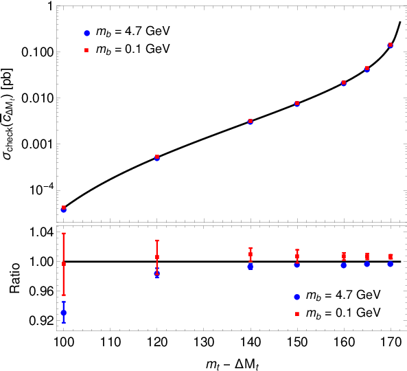
The result of our check is shown in Figure 9. Here, we have rearranged the contributions as follows,
| (6.1) | |||||
| (6.2) |
where is the contribution to the non-resonant part from the diagram at NLO (Figure 1) in the presence of the complementary cut. The line in Figure 9 shows our semi-analytical result for obtained by means of (6.1). The points show the same quantity determined by evaluating (6.2) using MadGraph. The contribution from diagram is included in , because our edited MadGraph code, described in Section 5.1, corresponds to the combination that appears in (6.2). We performed the same check for the individual contributions from the diagrams with . In particular, this provides very welcome reassurance that the scheme dependence within part (III) has been treated consistently. Within estimated numerical errors we find good agreement, if the bottom-quark mass is neglected, as is done in our calculation.
6.2 Implementation in QQbar_Threshold
All of the aforementioned NNLO corrections have been implemented in the new version 2 of the public code QQbar_threshold [32]. A summary of the code changes and some code examples for the new functions are provided in Appendix A. QQbar_threshold can be downloaded from https://www.hepforge.org/downloads/qqbarthreshold/. An updated online manual is available under https://qqbarthreshold.hepforge.org/.
6.3 Comparison to other approaches
While a complete calculation of NNLO electroweak and non-resonant contributions to the top-pair threshold as reported here has never been done before, NNLO non-resonant corrections have been evaluated in certain approximations in [50] and [31]. We briefly comment on these approximations and their limitations here.
6.3.1 Comparison to [50]
The leading NNLO non-resonant contributions for the case of “not-too-loose” cuts satisfying were determined in [50] within the so-called phase-space matching (PSM) approach. This result captures the first terms in the expansion in () of the full non-resonant result, namely the terms of order , and . The latter correspond to the endpoint-divergent terms computed in [27], which give the approximate result labelled “aNNLO” in Figure 14 below. Because of the “not-too-loose” cut condition, the PSM approach does not allow the calculation of the total cross section near the top anti-top threshold.
The agreement between the PSM result and the full non-resonant computation of the non-analytic terms in the expansion in the invariant-mass cut parameter can be understood as a consequence of the cancellation of singularities between adjacent regions of loop momentum [27]. The non-resonant terms are obtained in the PSM approach by computing the ultraviolet behaviour of the resonant amplitude where the cut on the invariant mass of the top and anti-top quark has been implemented. Therefore effectively acts as a regulator of the ultraviolet singular behaviour of the resonant part of the amplitude, that is obtained assuming on-shell top quarks, when the latter is further taken into the off-shell limit, i.e. for . On the other hand, the endpoint-divergent terms are obtained from the non-resonant part of the amplitude, that assumes off-shell tops with , upon going to the (infrared) on-shell limit within a distance regulated by . The fact that both expansions provide the same divergent terms in is thus a consequence of the cancellation of the dependence on the cut-off that separates the resonant and non-resonant regions. For the limitations on the PSM result to provide higher-order terms in the expansion we refer the reader to [27].
6.3.2 Comparison to [31]
Another approach, introduced in [31], aims at the computation of the non-resonant contribution to the total cross section in an expansion in , where is treated as a small parameter. Even though is not small in reality, one may hope that with sufficiently many terms in the expansion, a good approximation might be obtained. Indeed, the exact NLO non-resonant result from [26] was reproduced by combining a deep expansion with Padé approximants.
Our concern here is the computation of the first two terms in the expansion of the NNLO non-resonant contribution. In the present notation, the first term in the expansion given in [31] reads explicitly
| (6.3) |
It is immediately clear from this expression that the meaning of “non-resonant” is different from ours, in which case the non-resonant contribution is analytic in energy and has a pole. It appears that [31] does not distinguish between what we call non-resonant and absorptive matching coefficient contribution to the resonant part and directly constructs the expansion of the diagram in , such that (6.3) gives the sum of all contributions at order .
It is instructive to construct the terms from the results in [30] and in the present paper. We find that they arise only from
| (6.4) |
in part (I) and specifically from diagrams and in . Each of the two terms contains a pole, which cancels in the sum. This holds separately for the two diagrams and plus their corresponding resonant counterparts1313 13 The resonant counterparts of and correspond to the same diagrams but taking the loop momenta in the top anti-top loops in the potential region, and keeping only the NNLO term of the self-energy insertion in . that contribute to . We note that the leading term (6.3) from [31] originates only from diagram . Our result for this diagram including its resonant counterpart indeed agrees with the above except for the constant term (see (C.4), (C.5) in Appendix C). However, as was already mentioned in [27, 30], contrary to the statement made in [31] there is a non-vanishing contribution from at the same order. We computed the from this diagram explicitly, and find that the complete contribution to the total cross section reads
| (6.5) |
Note the absence of a logarithmic dependence on in the sum of all contributions (see (C.4)–(C.7) for the individual results). This can be traced to the cancellation of divergences and the scaling of the leading momentum regions that contribute to the enhanced term. Furthermore, the coefficient of differs by a factor of two, which is related to the contribution of the diagram as described in Appendix C. We therefore disagree with the NNLO non-resonant result given in [31] already from the leading term in the expansion.
The authors of [31] did not actually attempt the calculation of diagram but referred to [54] to claim that it must not contribute. However, as already discussed in Section 3.1.2, the purported vanishing of , called “jet-jet” contribution in [54], refers to a different order in the non-relativistic expansion, namely NLO, and is reflected in the present framework as the non-renormalization of the coupling of the top quark to a potential gluon and the Coulomb potential by electroweak effects. Moreover, when the expansion is constructed from momentum regions, the leading term arises from a momentum region that was missed in [31]. Further details on the comparison and diagram can be found in Appendix C.
7 Discussion of results
Recent experimental studies [2, 3] concluded that the statistical uncertainties of the top threshold scan at a future collider can be very small in realistic running scenarios. Thus, when discussing the impact of the electroweak and non-resonant corrections in this section, we focus on the theoretical uncertainties. An experimental analysis based on the theory prediction available in QQbar_threshold [32] is in progress [4] and will combine statistical and systematic experimental errors with theory uncertainties.
To avoid the IR renormalon ambiguities, we exclusively employ the PS shift (PSS) mass scheme defined in [14, 59, 32]. For the numerical evaluation we adopt the input values
| (7.1) |
where is the top-quark PS mass [76] and the running electroweak coupling is taken from [60], see the discussion in Section 3.1.4.
7.1 Size of the electroweak effects

We define a reference QCD prediction by adding the small P-wave contribution [22] to the S-wave result of [9]. The result is shown by the grey hatched band labelled “QCD” in Figure 10, which is spanned by variation of the renormalization scale between 50 GeV and 350 GeV. Figure 10 also shows the net effect of all the corrections discussed above, excluding ISR, which will be considered below. These non-QCD effects slightly increase the height of the peak and move it towards smaller center-of-mass energies. Above the peak the cross section is slightly decreased by about . Overall, the effect of the non-QCD corrections is to make the resonance more pronounced. The largest effect is observed below the peak, where the absorptive parts of the matching coefficients and the non-resonant contribution dominate the non-QCD corrections. Here, the bands cease to overlap at around GeV. The size of the uncertainty band is somewhat increased and now reaches up to directly below the peak, where the uncertainty estimate for the QCD result is . In the remaining regions it is about . The increase of the scale uncertainty is mainly due to the Higgs potential insertion as was already observed in [25].
The size of the individual contributions is shown in Figure 11. We have already discussed the Higgs, QED Coulomb and NLO non-resonant corrections in [25], but briefly recapitulate the results here to give a complete overview over the non-QCD correction up to NNLO. In the top-panel we show the relative effect of the Higgs contribution at NNLO and NNNLO. At NNLO there is an almost constant relative shift, because only the hard-matching coefficient is present. At NNNLO, there is also a contribution from the local Higgs potential, which modifies the position of the peak. Due to the attractive nature of the potential, the binding energy is increased and the peak is shifted to the left. At the same time the Higgs corrections increase the cross section by , depending on the value of , and make the peak more pronounced. The comparison of the dashed and solid curves demonstrates that the inclusion of the NNNLO corrections is important for correctly capturing the energy dependence of the Higgs effects, which is crucial for a reliable measurement of the top Yukawa coupling.
The remaining electroweak contributions to the ‘partonic’ resonant cross section, , , , , are shown in the middle panel. The dashed line corresponds to the correction from the QED Coulomb potential only. It is attractive and therefore leads to an increase of the cross section by and a shift of the peak towards smaller center-of-mass energy. The solid line shows the full correction. The width contribution decreases the cross section by depending on the energy. Including the real part of the electroweak matching coefficient leads to an almost constant relative shift of about . The absorptive part of the matching coefficient multiplies the real part of the non-relativistic Green function, which has a broad peak, roughly centered around the point where the imaginary part has its maximal slope, on top of a smooth background. Thus, the absolute contribution has only a mild energy dependence and is of the order of near and above the peak. However, it becomes even more important below the peak, where the cross section is small and modified by up to .
The lower panel illustrates the behaviour of the non-resonant contribution to the total cross section. Its absolute size is nearly energy-independent. Thus, the shape of the curves is given by the “inverse” of the resonant cross section. At NLO, the effect is of the order near and above the peak and reaches up to for low center-of-mass energies, where the resonant cross section becomes small. The NNLO corrections compensate about of the NLO result. This is in contrast to the findings of [27, 30], where an enhancement of the negative non-resonant correction from an approximate NNLO result was observed. The apparent discrepancy is entirely explained by the very different choice made in [27, 30] for the finite-width scale (GeV) compared to the present (GeV). The dependence of the full result on is very mild as discussed below and, thus, mainly the size of the individual contributions is affected – most notably the non-resonant correction and the one from the absorptive part of the hard matching coefficients.

We recall that the bands in Figure 10 only include the variation of the renormalization scale between 50 GeV and 350 GeV, while the scale GeV is kept fixed. The dependence on the scale cancels exactly between all contributions of a given order. We show the dependence of the resonant cross section and the full cross section in Figure 12. For the resonant-only cross section, it is mild near and above the peak, but is significantly larger than the renormalization scale dependence below the peak. The sensitivity to is greatly reduced for the full cross section, where the variation between 20 and 700 GeV considered in the plots only yields a effect near and above the peak and only a mild below the peak. The remaining dependence is of NNNLO, where the full QCD corrections, but only a few electroweak effects are included and therefore no full cancellation is achieved.
The central value for the finite-width scale is chosen near the hard scale to make the corresponding logarithms in the non-resonant part small. The logarithms of are introduced by the separation into different momentum regions and are therefore spurious in nature. Explicitly, some of the ‘large’ logarithms contained in the full cross section are split as follows
| (7.2) |
where the first logarithm to the right of the equality sign is part of the non-resonant contribution and the second one of the resonant. Choosing captures the ‘large’ logarithms present at NNNLO in the resonant part and renders the logarithms contained in the non-resonant part small. While the NNNLO resonant contributions are already partially known, the NNNLO non-resonant corrections are beyond the present computational limits. Thus our scale choice minimizes the uncertainty from the missing NNNLO contributions.1414 14 The same argument motivated the different choice made in [27, 30], since in these papers the NNLO resonant electroweak contribution was not available.
Variation of the scale can be used to estimate the size of the missing NNNLO non-resonant corrections. The corresponding bands for the resonant plus NLO non-resonant and full cross section are shown in Figure 13, where we have varied between 20 and 700 GeV. We observe that the inner (red) band is entirely contained in the outer (grey) one and much narrower. Thus, the chosen range of the finite-width scale variation provides a reasonable estimate of the NNLO non-resonant correction. However, an estimate of the missing NNNLO non-resonant correction based on the width of the “full” (red) band in Figure 13 is potentially less reliable, because the leading NNNLO terms might not cause any dependence. This would be similar to the situation at NLO, where the leading non-resonant effect arises, yet there is no dependence of the resonant contribution at this order at all, since the divergence from factorizing resonant and non-resonant contributions is purely linear.
We discussed the possibility of imposing loose cuts, which affect only the non-resonant part of the cross section, in Section 2.3. The dependence on the cut defined in (2.14) is shown in Figure 14, where the dotted and solid lines denote the NLO and NNLO non-resonant contribution. Very loose cuts with GeV have only a mild influence on the cross section. Tighter cuts GeV reduce the cross section by pb. We observe that for around 4 GeV the NNLO non-resonant contribution becomes as large as the NLO one. Here, the assumption that the cut is loose is no longer appropriate and our description breaks down. The dashed line in Figure 14 shows the approximate NNLO result [27], which includes only the endpoint-divergent terms as , for comparison. It describes the dependence on the cut very well, since the endpoint-divergent terms are most sensitive to it, but it is shifted by -0.004 pb for the full cross section and up to -0.013 pb including invariant mass cuts. In the absence of any cuts the exact result corresponds to a correction with respect to the approximate NNLO result. We note, however, that for the scale choice of [27] and in the range of loose, but not too loose cuts the approximation is much better.

We finally discuss the effects of initial-state QED radiation, which have so far only been taken into account in the experimental studies. Figure 15 shows the partonic cross section and its convolution with the electron structure functions. The QED contribution to the partonic cross section from (3.64) is a small effect of the order . The convolution, however, reduces the cross section by . The black band is spanned by four different implementations of the convolution (3.53) of the full NNNLO QCD plus NNLO EW cross section with the structure functions. This involves an extrapolation of the cross section for energy values outside of the range of the grids available in QQbar_Threshold[32]. We either use the shape of the LO cross section below GeV, rescaled to match the full result at GeV, or an alternative implementation that interpolates linearly between pb and our result at GeV. Numerically, we find a small difference of near and above the peak, which goes up to at GeV.1515 15 While the grid could technically be extended to smaller values of , the PNREFT and unstable-particle EFT breaks down far below the threshold. Improving the accuracy in this region would require matching the EFT description to the fixed-order calculation of the full non-resonant process as discussed for a single-particle resonance in [35, 36]. For both extrapolations we consider the convolution (3.53) with the structure functions as defined in (3.60) and a purely LL approximation where we set in the structure function and accordingly modify the non-logarithmic ISR contribution (3.64) for the different subtraction term (3.63). The difference is formally a NLL effect and provides a rough estimate of the overall size of NLL ISR corrections. It amounts to about % above the peak and reaches up to in the region where the slope is large.
For comparison we furthermore show as the dashed line the expression
| (7.3) |
where the ISR resummation is only applied to the LO cross section. Since the LL resummation modifies a NkLO correction by order one, the difference between ISR and ISR0 is formally a NLO effect. This emphasizes that it is mandatory to perform the convolution with the full partonic result.
We see, as it is of course expected, that ISR is a huge effect, reducing the cross section by . It also leads to a significant modification of the shape. The peak is shifted by almost 200 MeV to the right and smeared out considerably. Its height is reduced by about 40%. This emphasizes the need for a full NLL treatment of ISR and a proper analysis of the convergence and remaining uncertainty, which is of universal importance for high-energy collider processes, but beyond the scope of this work. We further note that at the level of NNLO electroweak accuracy the partonic cross section depends on the scheme employed for the electron structure function, and a phenomenological convolution as often applied in experimental studies in an unspecified scheme is no longer adequate.
7.2 Sensitivity to Standard Model parameters

Since the non-QCD effects computed in this paper cause substantial corrections to the cross section we provide an update of the discussion in [9, 25] of the sensitivity of the top threshold scan to Standard Model parameters. Figures 16, 17 and 18 estimate the sensitivity by comparing the effects of parameter variations to the scale uncertainty in terms of the relative variation to a reference cross section.

All electroweak and non-resonant effects discussed in this paper are included in the figures, in particular also the ISR corrections. There are small quantitative differences with respect to [9, 25], such as a small reduction of the height of the peaks present in the top-mass variation curves near 344.5 GeV, but the essence of the results and the associated conclusions remain unchanged. It is especially noteworthy that the huge ISR correction discussed above does not degrade the sensitivity. Since the bulk of the ISR correction is produced by the convolution with the luminosity function, we expect that the additional convolution of the cross section with the collider-specific beam function will not dilute the sensitivity to the parameters, either.
From Figures 16 and 17 we expect the threshold scan to be sensitive to variations of about MeV for the top-quark PS mass, MeV for the top-quark width, for the top-quark Yukawa coupling and for the strong coupling constant , when only a single parameter is varied at a time. These numbers are obtained from comparing the width of the band for the parameter variation with the one from the theoretical uncertainty, and requiring that the former is larger than the latter for a sufficient range in energy. This leaves open the question of how well the corrections from the simultaneous variation of several parameters can be disentangled from their energy dependence, which particularly concerns the Yukawa and the strong coupling, where variations lead to similar effects as seen in Figure 17 for the energy dependence and in Figure 18 for the position and height of the peak in the cross section. This needs to be addressed within realistic simulations, which include experimental uncertainties as well.
8 Conclusions
The recent advance in the QCD calculation of the top anti-top threshold [9] has motivated the consideration of non-QCD effects of potentially similar size to the third-order QCD correction. While Higgs/top-Yukawa coupling effects up to the third order were already obtained in [25], the present work completed the calculation of NNLO electroweak corrections and in particular the NNLO non-resonant contribution to the process near the top-pair production threshold. This elevates the theoretical prediction to NNNLO QCD plus NNLO electroweak accuracy, including for the first time initial-state radiation in a scheme consistent with one-loop QED corrections. The new effects are indeed non-negligible compared to the accuracy estimated for the pure QCD calculation and are therefore essential for accurate top and Standard Model parameter determinations from the threshold. They have been implemented in the new version 2 of the public code QQbar_threshold [32].
Despite the level of sophistication already achieved, further improvement could be considered or might be necessary, such as the combination of the NNLL summation of logarithms of in the QCD part [24] with the NNNLO fixed-order calculation [9], the inclusion of already known NNNLO electroweak corrections (see [45, 47]) or the one-loop correction to the Higgs potential (a N4LO effect) together with the terms required to make these additions factorization-scheme independent. To cancel the finite-width scale dependence of the NNNLO QCD result completely, the non-resonant part is needed to the same accuracy, which appears prohibitive at present. Finally, a consistent implementation of QED initial-state radiation with next-to-leading logarithmic accuracy seems to be a general prerequisite for accurate predictions of scattering at a future high-energy collider.
Acknowledgements
We are grateful to B. Chokoufé Nejad, C. Degrande, R. Frederix, O. Mattelaer, J. Piclum, V. Shtabovenko, F. Simon, and J.F. von Soden-Fraunhofen for helpful discussions. We made use of Axodraw [79] and JaxoDraw [80] to draw Feynman diagrams. AM was supported by a European Union COFUND/Durham Junior Research Fellowship under EU grant agreement number 267209. PRF acknowledges financial support from the “Spanish Agencia Estatal de Investigacion” (AEI), the EU “Fondo Europeo de Desarrollo Regional” (FEDER) through the project FPA2016-78645-P, and from the grant “IFT Centro de Excelencia Severo Ochoa SEV-2016-0597”. MB and TR have been supported by the Gottfried Wilhelm Leibniz programme of the Deutsche Forschungsgemeinschaft (DFG), and the DFG cluster of excellence “Origin and Structure of the Universe.”
Appendix A Implementation in QQbar_threshold
The new NNLO corrections have been implemented in the
new version 2 of the public code QQbar_threshold.
In the following, we summarize the changes and give code examples for new
functions. QQbar_threshold can be downloaded from
An updated online manual is available under https://qqbarthreshold.hepforge.org/.
A.1 Non-resonant corrections
By default, the ttbar_xsection function now includes the NNLO non-resonant contribution to the cross section. The NLO and NNLO corrections can be controlled individually with the contributions option. For example,
will calculate the cross section with the NLO non-resonant correction multiplied by a_NLO and the NNLO correction multiplied by a_NNLO. The equivalent Mathematica code is
As before, the complete nonresonant contribution can be disabled by setting the option resonant_only to true ( ResonantOnly -> True in Mathematica).
A.2 Initial-state radiation
Initial-state radiation requires the computationally expensive convolution with structure functions. Therefore, this correction is not included automatically.
After defining the luminosity function
| (A.1) |
with the electron structure functions from (3.53) the cross section after initial-state radiation is given by
| (A.2) |
Here, is the partonic cross section including the non-logarithmic initial-state radiation correction (see (3.64)). The non-logarithmic correction can be included with the option setting
in C++ and ISRConst -> True in Mathematica. The default setting for this option is false. It should be set to true if (and only if) the logarithmically enhanced component of the initial-state radiation is also included via convolution with the luminosity function.
In principle, the convolution integral in (A.2) covers the whole energy range from zero to the nominal center-of-mass energy. However, our prediction for the cross section is only valid in the vicinity of the threshold. Sufficiently below the threshold the actual cross section becomes negligible. This implies that we can introduce a lower cut-off in the integral (cf. Section 7.1). In the following we choose .
A further, purely numerical problem arises from the integrable divergence of the luminosity function for . In order to eliminate this divergence, we can change the integration variable to and write the cross section as
| (A.3) |
with the modified luminosity function and a cut-off . The function is available in QQbar_threshold as ISR_log(sqrt_s, alpha) in C++ and ISRLog in Mathematica.
Finally, version 2 of QQbar_threshold provides an integrate function in the header integrate.hpp, which can be used to compute the convolution integral as shown below.
The following C++ code prints the cross section pb after initial state radiation for a center-of-mass energy of GeV, including all known perturbative corrections:
The corresponding Mathematica code is
Numerically, the structure function under the replacement is very close to the luminosity function. The same holds for the modified versions of both functions. Indeed, substituting modified_luminosity_function(t, beta) with modified_structure_function(t,2*beta) in the example changes the result for the cross section to pb, i.e. by less than . This observation can be used to somewhat accelerate the computation of the convolution at the cost of accuracy.
A.3 Width corrections
Among the resonant NNLO electroweak corrections listed in (3.12), only and are not already available in version 1 of QQbar_threshold. In version 2, the correction proportional to the top-quark width is included by default in the prediction for the cross section. Its components (cf. (3.19), (3.22)) can be controlled individually with the new contributions options v_width_kinetic (Eq. (3.18)), v_width2 (Eq. (3.17)), and width_ep (Eq. (3.21)). The respective Mathematica contribution names are vwidthkinetic, vwidth2, and widthep.
To incorporate the width corrections to the quarkonium energy levels from (3.35) the function ttbar_energy_level(n, mu, \{m, width\}, order, opts) can now take both the mass and width as arguments. Similarly, the ttbar_residue function can now take both arguments. In this way, this function includes the width corrections to the wave functions from (3.37). The corresponding Mathematica functions TTbarEnergyLevel and TTbarResidue are similarly extended. Finally, the toponium width including the corrections in (3.36) can be computed with the new function ttbar_width(n, mu, \{m, width\}, order,opts) (TTbarWidth in Mathematica).1616 16 This new function should not be confused with the older top_width function, which calculates the width of the top quark itself as opposed to the width of a toponium bound state.
A.4 Note on backwards compatibility
Disabling the new corrections in version 2 via the contributions option will produce results that are similar, but not identical to version 1 of the code. There are two causes for the difference.
First, as detailed in Sections 3.1.3 and 4.1, the calculational scheme for the NNLO electroweak corrections to the resonant cross section has been changed. Consequently, predictions for the cross section at or beyond NNLO that include electroweak corrections will differ between the two versions, even if all new corrections are disabled. The numerical differences are typically less than 1%, but can amount to almost 10% for a small renormalization scale and far below the threshold, where the cross section is already very small and the (new and old) NNLO electroweak corrections are sizeable.
Second, in contrast to the original code, version 2 now captures the full dependence on the scale . The numerical effect of this change is of the order of a few per mille for low energies and significantly less than one per mille in the peak region.
A.5 Calculation of the non-resonant correction
The dynamic numeric evaluation of the NNLO non-resonant corrections is computationally prohibitively expensive. Hence, QQbar_threshold internally uses interpolation of a precomputed grid. For reference purposes, a copy NNLO_nonresonant_grid.tsv of this internal grid is provided in the directory given by the function grid_directory in C++ and the variable GridDirectory in Mathematica. The coordinates of the grids are given by , accounting for variations of the top-quark mass, and , which covers changes in the invariant mass cut discussed in Section 2.3. The remaining two grid entries and parametrize the automated and the manual part of the non-resonant cross section for . To obtain their contribution to the cross section, these entries have to be multiplied by a factor of . The complete NNLO correction to the non-resonant cross section for arbitrary is then given by
| (A.4) |
where the coefficient of the logarithm reads
| (A.5) |
As mentioned before, the dependence on has to cancel exactly against the dependence in the resonant cross section. Like in the resonant part, we therefore do not expand out the energy dependence of the -channel propagators in . The last term in (A.4) is required because we have expressed the non-resonant cross section in terms of the all-order width . The NLO non-resonant part is proportional to and therefore implicitly contains the NNLO correction , where is the NLO QCD correction to the top-quark width. The same contribution appears in the NNLO calculation of the non-resonant part and we must include the last term in (A.4) to subtract this double counting.
Note that highly unphysical top-quark masses, i.e. or and extremely tight invariant mass cuts are not supported. Furthermore, the default values are assumed for the remaining Standard Model parameters, such as the values of and .
Our code for producing the NNLO non-resonant grid depends on a number of software packages, including MadGraph5_aMC@NLO [41], FastJet [77], and Cuba [78]. In order to facilitate reproducing our results without having to install all dependencies, we provide an image that can be executed using the Docker virtualisation software. After installing Docker and downloading the image nnlo_nonres_grid_entry.tar.gz from https://www.hepforge.org/downloads/qqbarthreshold/, it can be imported with
and run with
with xw and yw replaced by the respective values for the parameters introduced above. The last line of the output corresponds to a grid entry in the same format as in the reference grid.
For convenience we provide a Mathematica interface to the calculation of the NNLO non-resonant grid entries. After importing the Docker image as described above and loading the QQbarGridCalc Mathematica package distributed with QQbar_threshold, a grid entry can be computed with
which returns a list . Setting the Verbose option to False will suppress intermediate output.
Especially for large values the calculation of the automated contribution can fail, in which case a slight change in the input parameters may help. In practice, this is not a severe problem as the automated contribution becomes essentially constant in this region. The precision of the automated calculation is not very high, and the values obtained can easily deviate from the ones in the reference grid by around . Since the NNLO non-resonant contribution itself is not very large and typically dominated by the manual and logarithmic contributions, this translates to an error of at most one per mille in the final cross section. One way to reduce this error further would be to calculate the grid entries several times and average over the results.
In principle it is possible to compute an entirely new grid with the Docker container. In practice it is computationally much more efficient to calculate in the absence of an invariant mass cut, i.e. for , and derive the entries for all other values of exploiting complementary cuts as discussed in Section 2.3. The entry for some with is then given by , where the phase space integral in is restricted to the complementary region . In this way, the numerically problematic endpoint region is only computed once for each value of .
Appendix B Implementation of the subtractions in MadGraph
We briefly describe the implementation of the subtractions of the diagram in Figure 1 and all the diagrams in Figures 2 and 3 in MadGraph5_aMC@NLO 2.5.0.beta2. The MG5_aMC code for the computation of the process at NLO in QCD is created in the directory TBWsubtractions by entering the commands
in the MadGraph5 prompt. First, we subtract the diagram from the code in the directory /SubProcesses/P0_epem_wmtbx/.1717 17 Here and in the following / refers to the code directory. To this end, we identify the corresponding diagram numbers in MadGraph as 3 and 4 using born.ps. The subtraction is achieved by removing the terms proportional to AMP(I)*DCONJG(AMP(J))* with I,J in the squared matrix element. This affects the function BORN in born.f and BORN_HEL in born_hel.f. We note that one should avoid first adding and then subtracting the terms to avoid numerical instabilities since these contributions are divergent at threshold.
To subtract the real corrections in Figure 2 we remove the respective terms in the squared real amplitude given by the function MATRIX_1 in matrix_1.f where the corresponding set of I,J values can be determined from matrix_1.ps. To maintain separate IR finiteness of the real and virtual contributions we also have to edit the FKS subtraction terms in the files b_sf_001.f, b_sf_002.f, and b_sf_003.f accordingly. This is done by removing the terms containing the product of the tree-level amplitudes 3 and 4 in the functions B_SF_00i.
In the folder /SubProcesses/P0_epem_wmtbx/V0_epem_wmtbx for the virtual corrections we first apply the usual subtractions for the squared tree-level amplitude to the function MATRIX in born_matrix.f. The interference of a given one-loop diagram with the tree-level diagrams is evaluated by the function CREATE_LOOP_COEFS in polynomial.f. We create a copy called CREATE_LOOP_COEFS_h1bcd and which is modified by removing the interference with the tree-level diagrams 3 and 4. This allows us to remove the diagrams and with by modifying the calls to CREATE_LOOP_COEFS in coef_construction_1.f for the loop diagrams corresponding to the left-hand sides of the cuts. We either add the suffix h1bcd or comment out the calls. Again the relevant diagram numbers in MadGraph can be identified from the graphical representation loop_matrix.ps. The same changes are applied to the multiple precision version of the virtual corrections given in mp_compute_loop_coefs.f and mp_coef_construction_1.f.
Last but not least one needs to modify the counterterms given in loop_matrix.f. The identification of the Madgraph IDs of the counterterm diagrams is more complicated since they are not drawn but must be inferred from the code. The counterterm amplitudes AMPL(K,I), where the first index K denotes the finite part, the pole and the pole, are defined in helas_calls_ampb_1.f and helas_calls_uvct_1.f. The first file contains -terms and mass renormalization counterterms which are attributed to the loop diagrams in the same order in which they appear in loop_matrix.ps. The second file contains the multiplicative wave function renormalization counterterms for the tree-level diagram. To subtract the diagrams and the contributions of the remaining diagrams in the squared contribution we remove the terms proportional to AMPL(K,I)*DCONJG(AMP(J))* with I and J in the function SLOOPMATRIX in loop_matrix.f.
In addition we can implement the minimal subtraction of the UV divergences in with by modifying the interference of the divergent part of the wave function renormalization of the tree-level diagrams 3 and 4 with the other tree-level diagrams. Explicitly, we multiply AMPL(2,I) with I in the subroutine HELAS_CALLS_UVCT_1 in helas_calls_uvct_1.f with a factor . As discussed in Section 5.1 the -terms and finite parts of the wave function renormalization contributions for the interference contribution are not modified. Alternatively, one can simply deactivate the check for UV finiteness which yields the same results.
Following the discussion in Section 5.1 we have to deactivate an internal MadGraph consistency check for the positivity of the squared real amplitude to make the modified code run without producing error messages. This is done by removing the code block
in /SubProcesses/fks_singular.f. Older MadGraph versions also require modifications in the file /SubProcesses/P0_epem_wmtbx/BinothLHA.f to allow for negative values of the squared Born amplitude.
Our modified version of the MadGraph code is shipped with the grid generation routines in the new version of QQbar_Threshold. We have checked our procedure by applying similar modifications to the process generated with the older MadGraph version 2.4.3. Furthermore, we have verified that an analogous set of changes correctly removes the -boson exchange contribution to the process at NLO by comparing the results to the ones obtained by excluding the -boson exchange already in the process generation.
Appendix C Further details on the comparison to [31]
We extend in this appendix the discussion about the discrepancy with the result for the cross section at leading order in the expansion of [31] and its connection to diagram . First we explain why the cancellation of finite-width and endpoint divergences requires a non-vanishing contribution from diagram at leading order. A similar argument was already put forward in [27, 30]. Then we show that the leading-order term in comes from a loop-momentum region which is not among those considered to construct the unstable top EFT formulated in [31].

The NNLO resonant corrections related to and are given by the diagrams displayed in Fig. 19, where the loop-momenta in the top anti-top loops are expanded according to the potential () scaling, while the loop momentum in the loop is hard (). It should be understood that in the diagram with the self-energy insertion in the propagator one has to consider only the NNLO piece (the cut self-energy in the on-shell limit gives the top-quark width, which is a LO contribution since in the potential region; such terms are already accounted for by the replacement in the non-relativistic propagator). The diagram with the cut self-energy contributes to (3.22) and (3.44), once the symmetric diagrams are considered. In particular, the latter arises from field renormalization due the absorptive part of the electroweak one-loop self-energy. We have isolated that contribution in the second line of Figure 19, and split it such that one half of it can be attributed to field renormalization of the top quark leaving the production vertex, and the other half to the renormalization of the top-quark field entering the vertex. The latter contribution is exactly cancelled by the electroweak correction to the Coulomb potential (third diagram in the second line of Figure 19), because upon expanding out the external (potential) momenta from the self-energy and vertex loops, these diagrams are equivalent to the renormalized vertex in the on-shell scheme for zero transfered momentum (see Figure 5). Therefore, the resonant counterpart of is equal to minus one half of the diagram with the field renormalization of the top quark leaving the production vertex, which is proportional to the coefficient written in (3.44). It can be easily checked that behaves as , and that the contribution to the cross section contains a divergence from the real part of the Green function. Therefore both resonant diagrams in the first line of Figure 19 contain divergences, that are cancelled with endpoint divergences from the corresponding non-resonant diagrams and as was shown by explicit computation in [30]. In [31] only the non-resonant diagram analogue to is considered, while it is argued that the analogue to must vanish quoting results from [54]. As already explained in Section 6.3, the results from the latter refer to the vanishing of resonant contributions related to the top-quark instability at NLO, while the contribution under discussion here is of NNLO.

The dominant terms in the expansion can also be obtained upon application of the method of regions [37, 38]. Let us consider the forward scattering diagram in Figure 20, whose imaginary part corresponds to the sum of cut diagrams and (plus left-right symmetric ones), since no other cuts are kinematically possible. The authors of [31] discuss the contributions from the regions that are obtained by replacing in the hard, soft, potential and ultrasoft region. However, for the case of the diagram in Figure 20, which is related to discussed above, it can be shown that the leading order contribution comes from an additional region with parametrically smaller virtuality or order , that was not considered in [31]. With the momentum assignment of Figure 20, it corresponds to , and . We obtain for the relevant scalar integrals in this region:
| (C.1) | |||||
The relevant cases are ,
| (C.2) | |||||
| (C.3) |
Both scalar integrals produce a contribution of order to the cross section1818 18 A factor , where the term arises from the bottom propagators, appears in the numerator that comes along . The numerator of the term has no suppression. Hence when is extracted as in (C.4)–(C.8) below, both terms contribute at order . and the imaginary part contains a divergence, which are the properties that are needed to cancel the finite-width divergence at the leading order in the expansion discussed above. We also note that a non-vanishing contribution from the region , and , is consistent with the findings of [30], which identified that the leading-order term in of diagram originates from the region in the -integration , where adopting the momentum assignment of Figure 20.
For completeness, we finally provide results for the individual contributions to the cross section from diagrams and and their resonant counterparts at the leading order in :
| (C.4) | |||||
| (C.5) | |||||
| (C.6) | |||||
| (C.7) |
with
| (C.8) |
The sum of the non-resonant contributions and agrees with the result given in [30] if one takes into account that the leptonic tensor was treated in dimensions there, which introduces a factor compared to the result used in the present work.1919 19 We take the opportunity to correct a typo in [30]: a factor was missed in the hadronic tensor written in Eq. (3) therein.
References
- [1] K. Fujii et al., Physics Case for the International Linear Collider, arXiv:1506.05992 [hep-ex].
- [2] K. Seidel, F. Simon, M. Tesar and S. Poss, Top quark mass measurements at and above threshold at CLIC, Eur. Phys. J. C 73 (2013) no.8, 2530, arXiv:1303.3758 [hep-ex].
- [3] T. Horiguchi, A. Ishikawa, T. Suehara, K. Fujii, Y. Sumino, Y. Kiyo and H. Yamamoto, Study of top quark pair production near threshold at the ILC, arXiv:1310.0563 [hep-ex].
- [4] F. Simon, Impact of Theory Uncertainties on the Precision of the Top Quark Mass in a Threshold Scan at Future Colliders, PoS ICHEP 2016 (2017) 872, arXiv:1611.03399 [hep-ex].
- [5] M. Butenschoen, B. Dehnadi, A. H. Hoang, V. Mateu, M. Preisser and I. W. Stewart, Top Quark Mass Calibration for Monte Carlo Event Generators, Phys. Rev. Lett. 117 (2016) 232001, arXiv:1608.01318 [hep-ph].
- [6] A. Andreassen and M. D. Schwartz, Reducing the Top Quark Mass Uncertainty with Jet Grooming, JHEP 1710 (2017) 151, arXiv:1705.07135 [hep-ph].
- [7] I. I. Y. Bigi, Y. L. Dokshitzer, V. A. Khoze, J. H. Kühn and P. M. Zerwas, Production and Decay Properties of Ultraheavy Quarks, Phys. Lett. B 181 (1986) 157.
- [8] V. S. Fadin and V. A. Khoze, Threshold Behavior of Heavy Top Production in Collisions, JETP Lett. 46 (1987) 525 [Pisma Zh. Eksp. Teor. Fiz. 46 (1987) 417].
- [9] M. Beneke, Y. Kiyo, P. Marquard, A. Penin, J. Piclum and M. Steinhauser, Next-to-Next-to-Next-to-Leading Order QCD Prediction for the Top Antitop -Wave Pair Production Cross Section Near Threshold in Annihilation, Phys. Rev. Lett. 115 (2015) 192001, arXiv:1506.06864 [hep-ph].
- [10] M. Beneke, Y. Kiyo and K. Schuller, Third-order correction to top-quark pair production near threshold I. Effective theory set-up and matching coefficients, arXiv:1312.4791 [hep-ph].
- [11] P. Marquard, J. H. Piclum, D. Seidel and M. Steinhauser, Three-loop matching of the vector current, Phys. Rev. D 89 (2014) 034027, arXiv:1401.3004 [hep-ph].
- [12] M. E. Luke and M. J. Savage, Power counting in dimensionally regularized NRQCD, Phys. Rev. D 57 (1998) 413, [hep-ph/9707313].
- [13] M. Beneke, Y. Kiyo and K. Schuller, Third-order Coulomb corrections to the S-wave Green function, energy levels and wave functions at the origin, Nucl. Phys. B 714 (2005) 67 [hep-ph/0501289].
- [14] M. Beneke, Y. Kiyo and K. Schuller, Third-order correction to top-quark pair production near threshold II. Potential contributions, always in preparation.
- [15] M. Beneke and Y. Kiyo, Ultrasoft contribution to heavy-quark pair production near threshold, Phys. Lett. B 668 (2008) 143, arXiv:0804.4004 [hep-ph].
- [16] S. Wüster, Heavy quark potential at order [in German], Diploma Thesis, RWTH Aachen University (2003).
- [17] B. A. Kniehl, A. A. Penin, M. Steinhauser and V. A. Smirnov, Non-abelian heavy quark anti-quark potential, Phys. Rev. D 65 (2002) 091503 [hep-ph/0106135].
- [18] M. Beneke, Y. Kiyo, P. Marquard, A. Penin, J. Piclum, D. Seidel and M. Steinhauser, Leptonic decay of the (1) meson at third order in QCD, Phys. Rev. Lett. 112 (2014) no.15, 151801, arXiv:1401.3005 [hep-ph].
- [19] C. Anzai, Y. Kiyo and Y. Sumino, Static QCD potential at three-loop order, Phys. Rev. Lett. 104 (2010) 112003, arXiv:0911.4335 [hep-ph].
- [20] A. V. Smirnov, V. A. Smirnov and M. Steinhauser, Three-loop static potential, Phys. Rev. Lett. 104 (2010) 112002, arXiv:0911.4742 [hep-ph].
- [21] R. N. Lee, A. V. Smirnov, V. A. Smirnov and M. Steinhauser, Phys. Rev. D 94 (2016) 054029, arXiv:1608.02603 [hep-ph].
- [22] M. Beneke, J. Piclum and T. Rauh, P-wave contribution to third-order top-quark pair production near threshold, Nucl. Phys. B 880 (2014) 414, arXiv:1312.4792 [hep-ph].
- [23] A. H. Hoang et al., Top - anti-top pair production close to threshold: Synopsis of recent NNLO results, Eur. Phys. J. direct C 3 (2000) 1 [hep-ph/0001286].
- [24] A. H. Hoang and M. Stahlhofen, The Top-Antitop Threshold at the ILC: NNLL QCD Uncertainties, JHEP 1405 (2014) 121, arXiv:1309.6323 [hep-ph].
- [25] M. Beneke, A. Maier, J. Piclum and T. Rauh, Higgs effects in top anti-top production near threshold in annihilation, Nucl. Phys. B 899 (2015) 180, arXiv:1506.06865 [hep-ph].
- [26] M. Beneke, B. Jantzen and P. Ruiz-Femenía, Electroweak non-resonant NLO corrections to in the resonance region, Nucl. Phys. B 840 (2010) 186, arXiv:1004.2188 [hep-ph].
- [27] B. Jantzen and P. Ruiz-Femenía, Next-to-next-to-leading order nonresonant corrections to threshold top-pair production from collisions: Endpoint-singular terms, Phys. Rev. D 88 (2013) 5, 054011, arXiv:1307.4337 [hep-ph].
- [28] M. Beneke, P. Falgari, C. Schwinn, A. Signer and G. Zanderighi, Four-fermion production near the W pair production threshold, Nucl. Phys. B 792 (2008) 89, arXiv:0707.0773 [hep-ph].
- [29] S. Actis, M. Beneke, P. Falgari and C. Schwinn, Dominant NNLO corrections to four-fermion production near the W-pair production threshold, Nucl. Phys. B 807 (2009) 1, arXiv:0807.0102 [hep-ph].
- [30] P. Ruiz-Femenía, First estimate of the NNLO nonresonant corrections to top-antitop threshold production at lepton colliders, Phys. Rev. D 89 (2014) 097501, arXiv:1402.1123 [hep-ph].
- [31] A. A. Penin and J. H. Piclum, Threshold production of unstable top, JHEP 1201 (2012) 034, arXiv:1110.1970 [hep-ph].
- [32] M. Beneke, Y. Kiyo, A. Maier and J. Piclum, Near-threshold production of heavy quarks with QQbar_threshold, Comput. Phys. Commun. 209 (2016) 96, arXiv:1605.03010 [hep-ph].
- [33] A. Pineda and J. Soto, Effective field theory for ultrasoft momenta in NRQCD and NRQED, Nucl. Phys. Proc. Suppl. 64 (1998) 428 [hep-ph/9707481].
- [34] M. Beneke, A. Signer and V. A. Smirnov, Top quark production near threshold and the top quark mass, Phys. Lett. B 454 (1999) 137 [hep-ph/9903260].
- [35] M. Beneke, A. P. Chapovsky, A. Signer and G. Zanderighi, Effective theory approach to unstable particle production, Phys. Rev. Lett. 93 (2004) 011602 [hep-ph/0312331].
- [36] M. Beneke, A. P. Chapovsky, A. Signer and G. Zanderighi, Effective theory calculation of resonant high-energy scattering, Nucl. Phys. B 686 (2004) 205 [hep-ph/0401002].
- [37] M. Beneke and V. A. Smirnov, Asymptotic expansion of Feynman integrals near threshold, Nucl. Phys. B 522 (1998) 321 [hep-ph/9711391].
- [38] B. Jantzen, Foundation and generalization of the expansion by regions, JHEP 1112 (2011) 076, arXiv:1111.2589 [hep-ph].
- [39] J. Blümlein, K. H. Phan and T. Riemann, General -representation for scalar one-loop Feynman integrals, Nucl. Part. Phys. Proc. 270-272 (2016) 227, arXiv:1510.01063 [hep-ph].
- [40] E. Devetak, A. Nomerotski and M. Peskin, Top quark anomalous couplings at the International Linear Collider, Phys. Rev. D 84 (2011) 034029, arXiv:1005.1756 [hep-ex].
- [41] J. Alwall et al., The automated computation of tree-level and next-to-leading order differential cross sections, and their matching to parton shower simulations, JHEP 1407 (2014) 079, arXiv:1405.0301 [hep-ph].
- [42] J. Reuter, F. Bach, B. Chokoufé Nejad, A. Hoang, W. Kilian, M. Stahlhofen, T. Teubner and C. Weiss, Top Physics in WHIZARD, arXiv:1602.08035 [hep-ph].
- [43] M. Beneke, Perturbative heavy quark-antiquark systems, in: Proceedings of the 8th International Symposium on Heavy Flavor Physics (Heavy Flavors 8), 25-29 July 1999, Southampton, England, [hep-ph/9911490].
- [44] D. Eiras and J. Soto, Effective field theory approach to pionium, Phys. Rev. D 61 (2000) 114027, [hep-ph/9905543].
- [45] D. Eiras and M. Steinhauser, Complete Higgs mass dependence of top quark pair threshold production to order , Nucl. Phys. B 757 (2006) 197 [hep-ph/0605227].
- [46] A. H. Hoang and C. J. Reißer, Electroweak absorptive parts in NRQCD matching conditions, Phys. Rev. D 71 (2005) 074022 [hep-ph/0412258].
- [47] Y. Kiyo, D. Seidel and M. Steinhauser, corrections to the vertex at the top quark threshold, JHEP 0901 (2009) 038, arXiv:0810.1597 [hep-ph].
- [48] M. Beneke, P. Falgari and C. Schwinn, Threshold resummation for pair production of coloured heavy (s)particles at hadron colliders, Nucl. Phys. B 842 (2011) 414, arXiv:1007.5414 [hep-ph].
- [49] B. A. Kniehl and A. Sirlin, Pole Mass, Width, and Propagators of Unstable Fermions, Phys. Rev. D 77 (2008) 116012, arXiv:0801.0669 [hep-th].
- [50] A. H. Hoang, C. J. Reißer and P. Ruiz-Femenía, Phase Space Matching and Finite Lifetime Effects for Top-Pair Production Close to Threshold, Phys. Rev. D 82 (2010) 014005, arXiv:1002.3223 [hep-ph].
- [51] A. Czarnecki and K. Melnikov, Two loop QCD corrections to top quark width, Nucl. Phys. B 544 (1999) 520 [hep-ph/9806244].
- [52] K. G. Chetyrkin, R. Harlander, T. Seidensticker and M. Steinhauser, Second order QCD corrections to , Phys. Rev. D 60 (1999) 114015 [hep-ph/9906273].
- [53] M. M. Sternheim and J. F. Walker, Non-Hermitian Hamiltonians, Decaying States, and Perturbation Theory, Phys. Rev. C 6 (1972) 114.
- [54] K. Melnikov and O. I. Yakovlev, Top near threshold: All corrections are trivial, ??Phys. Lett. B 324 (1994) 217 ??[hep-ph/9302311].
- [55] B. Grzadkowski, J. H. Kühn, P. Krawczyk and R. G. Stuart, Electroweak Corrections on the Toponium Resonance, Nucl. Phys. B 281 (1987) 18.
- [56] R. J. Guth and J. H. Kühn, Top quark threshold and radiative corrections, Nucl. Phys. B 368 (1992) 38.
- [57] A. H. Hoang and C. J. Reißer, On electroweak matching conditions for top pair production at threshold, Phys. Rev. D 74 (2006) 034002 [hep-ph/0604104].
- [58] W. H. Furry, A Symmetry Theorem in the Positron Theory, Phys. Rev. 51 (1937) 125.
- [59] M. Beneke, A. Maier, J. Piclum and T. Rauh, The bottom-quark mass from non-relativistic sum rules at NNNLO, Nucl. Phys. B 891 (2015) 42, arXiv:1411.3132 [hep-ph].
- [60] F. Jegerlehner, Electroweak effective couplings for future precision experiments, Nuovo Cim. C 034S1 (2011) 31, arXiv:1107.4683 [hep-ph].
- [61] A. V. Manohar, Deep inelastic scattering as using soft collinear effective theory, Phys. Rev. D 68 (2003) 114019 [hep-ph/0309176].
- [62] E. A. Kuraev and V. S. Fadin, On Radiative Corrections to Single Photon Annihilation at High-Energy, Sov. J. Nucl. Phys. 41 (1985) 466 [Yad. Fiz. 41 (1985) 733].
- [63] M. Skrzypek, Leading logarithmic calculations of QED corrections at LEP, Acta Phys. Polon. B 23 (1992) 135.
- [64] W. Beenakker and A. Denner, Standard model predictions for pair production in electron - positron collisions, Int. J. Mod. Phys. A 9 (1994) 4837.
- [65] W. Beenakker et al., cross-sections and distributions, hep-ph/9602351.
- [66] H. H. Patel, Package-X: A Mathematica package for the analytic calculation of one-loop integrals, Comput. Phys. Commun. 197 (2015) 276, arXiv:1503.01469 [hep-ph].
- [67] R. Mertig, M. Böhm and A. Denner, FEYN CALC: Computer algebraic calculation of Feynman amplitudes, Comput. Phys. Commun. 64 (1991) 345.
- [68] V. Shtabovenko, R. Mertig and F. Orellana, New Developments in FeynCalc 9.0, Comput. Phys. Commun. 207 (2016) 432, arXiv:1601.01167 [hep-ph].
- [69] T. Hahn and M. Pérez-Victoria, Automatized one loop calculations in four-dimensions and D-dimensions, Comput. Phys. Commun. 118 (1999) 153 [hep-ph/9807565].
- [70] W. Beenakker, S. Dittmaier, M. Krämer, B. Plümper, M. Spira and P. M. Zerwas, NLO QCD corrections to t anti-t H production in hadron collisions, Nucl. Phys. B 653 (2003) 151 [hep-ph/0211352].
- [71] S. Frixione, Z. Kunszt and A. Signer, Three jet cross-sections to next-to-leading order, Nucl. Phys. B 467 (1996) 399 [hep-ph/9512328].
- [72] R. Frederix, S. Frixione, F. Maltoni and T. Stelzer, Automation of next-to-leading order computations in QCD: The FKS subtraction, JHEP 0910 (2009) 003, arXiv:0908.4272 [hep-ph].
- [73] G. Ossola, C. G. Papadopoulos and R. Pittau, On the Rational Terms of the one-loop amplitudes, JHEP 0805 (2008) 004, arXiv:0802.1876 [hep-ph].
- [74] G. ’t Hooft and M. J. G. Veltman, Regularization and Renormalization of Gauge Fields, Nucl. Phys. B 44 (1972) 189.
- [75] R. Frederix, private communication.
- [76] M. Beneke, A Quark mass definition adequate for threshold problems, Phys. Lett. B 434 (1998) 115 [hep-ph/9804241].
- [77] M. Cacciari, G. P. Salam and G. Soyez, FastJet User Manual, Eur. Phys. J. C 72 (2012) 1896, arXiv:1111.6097 [hep-ph].
- [78] T. Hahn, CUBA: A Library for multidimensional numerical integration, Comput. Phys. Commun. 168 (2005) 78 [hep-ph/0404043].
- [79] J. A. M. Vermaseren, Axodraw, Comput. Phys. Commun. 83 (1994) 45.
- [80] D. Binosi, J. Collins, C. Kaufhold and L. Theussl, JaxoDraw: A Graphical user interface for drawing Feynman diagrams. Version 2.0 release notes, Comput. Phys. Commun. 180 (2009) 1709, arXiv:0811.4113 [hep-ph].