Resonant production of and at the LHC
Abstract
We examine the production of and pairs at the LHC in the context of a Strongly Interacting Symmetry Breaking Sector of the Standard Model. Our description is based on a non-linear Higgs Effective Theory, including only the Standard Model particles. We focus on its scalar sector (Higgs boson and electroweak Goldstones associated to and ), which is expected to give the strongest beyond Standard Model rescattering effects. The range of the effective theory is extended with dispersion-relation based unitarization, and compared to the alternative extension with explicit axial-vector resonances. We estimate the and production cross-section, where an intermediate axial-vector resonance is generated for certain values of the chiral couplings. We exemplify our analysis with a benchmark axial-vector with TeV. Interestingly enough, these different approaches provide essentially the same prediction. Finally we discuss the sensitivity of ATLAS and CMS to such resonances.
1 Introduction
If physics beyond the Standard Model exists, the absence of new physics states in the few-hundred GeV region and the lightness of the new Higgs-like boson naturally suggest some new strongly interacting sector with an additional (pseudo) Goldstone boson beyond the three needed for the Electroweak Chiral Symmetry Breaking. This would call for enlarging the Standard Model (SM) symmetry group, leading perhaps to Composite Higgs Models.
A complete exploration of the Goldstone boson scattering in those SM extensions may provide important information on their underlying nature. This requires not only an examination of but also amplitudes, with . For , the scattering of longitudinal component of the massive electroweak (EW) gauge bosons is related to EW Goldstone () processes by the equivalence theorem (ET) [1, 2]: , . We will extract the latter amplitude within the ET regime and neglect the and masses. Furthermore, since numerically () 11 1 The top quark is not considered in this analysis and its impact in these scattering processes via loops deserves a separate dedicated analysis. Nonetheless, some estimates point out that these fermion corrections are subdominant [5, 6], as the scalar boson derivative interactions win eventually over the non-derivative Yukawa contributions. , all the masses of the remaining SM particles and their Yukawa couplings will also be neglected.
There are several approaches to describing a modified SM including a Strongly Interacting Symmetry Breaking Sector (SISBS). The existence of a large mass gap between the SM and possible new physics particles points out to effective field theories (EFT) as the most convenient and model independent framework for the study of beyond SM (BSM) scenarios. Likewise, we consider the non-linear representation of the EW Goldstones, as it provides the most general SM extension allowed by symmetry [3, 4]. Irrespective of the validity of those Composite Higgs Models (CHM), the scattering can be addressed in perturbation theory within the Higgs Effective Field Theory (HEFT) 22 2 Not to be confused with a similarly named earlier theory that required the top to be much heavier than the Higgs and consisted of an expansion in inverse powers of . [3, 7]. It describes the interactions of the would-be-Goldstone bosons from the spontaneous EW symmetry breaking. Following the CCWZ formalism [8] the transform non-linearly under chiral transformations and parametrize the coset , with the EW chiral group and the global custodial vector subgroup . HEFT extends the Higgsless Electroweak Chiral Lagrangian [9] by the addition of one singlet scalar Higgs field with generic couplings [7]; in this theory, one is agnostic about the nature of the Higgs, which is coupled as the most general scalar boson that does not disrupt the pattern of global electroweak symmetry breaking . Chiral symmetry is spontaneously broken down to the global custodial vector subgroup .
The subgroup is then gauged, like in the SM, and this introduces the coupling to the transverse gauge bosons (and thus, to the quark constituents of the proton). We will assume that the only source of custodial symmetry breaking is the gauging of the group and that additional breaking operators only appear at higher orders in the HEFT, being further suppressed.
In preparing this article we have kept in mind some recent hints in the searches in ATLAS [10], where a () local (global) significance excess has been reported at TeV. However, this excess has not been confirmed by CMS [11], so we do not commit to a fixed energy scale for any resonances. Nonetheless, we consider it useful to show that such phenomenon can be naturally described by the HEFT in the axial-vector channel with quantum numbers. Thus, as a case of study, we will consider a benchmark scenario with a resonance mass TeV and explore the feasibility of its search at the LHC.
The low-energy EFT is introduced in Sec. 2. In Sec. 3, we compute the most relevant LHC subprocess, , for the production of axial-vector resonances in the channel. Possible BSM effects are parametrized in an axial-vector form-factor defined therein. The strong rescattering in the HEFT, its unitarization and the generation of an axial-vector resonance are discussed in Sec. 4. The low-energy form-factor within the HEFT is computed in Sec. 5 and its extension up to the resonance region is provided in Sec. 6. For this, we consider models with alternative unitarization procedures or with explicit resonance Lagrangians, all of them leading to identical conclusions. In Sec. 7 we perform a phenomenological analysis of the production cross section at the LHC for the referred SISBS benchmark point, with an TeV resonance. Finally, some concluding remarks are provided in Sec. 8.
2 Low-energy EFT
2.1 Leading order Lagrangian
At leading order, the Lagrangian of the scalar symmetry breaking sector (SBS), the modified SBS of the SM, is an gauged non-linear sigma model HEFT which includes the Higgs field as a singlet. Including chirally interacting fermions, the lowest order (LO) SISBS Lagrangian reads
| (1) | |||
where the matrix field describes the EW would-be Goldstone fields (thus, by the ET, it gives us the , terms of the Lagrangian) and parametrizes the coset .
The matrix is equivalently described by any unitary matrix that fulfills . In particular, in the spherical representation, the would-be Goldstone fields are parametrized in the form
| (2) |
where and TeV the Higgs vacuum expectation value (vev).
The covariant derivative is then given by
| (3) |
In turn, the Higgs potential and the functions and are taken to have an analytical expansion in powers of around
| (4) |
In the SM one has , , , , and . Deviations from these values imply new physics.
Even though the low-energy parameters could be determined from the underlying theory if it was known, from a bottom-up approach the effective couplings are in principle independent from each other and must be extracted from experimental data. Furthermore, one naturally expects that some parameters are larger than others as specific low-energy couplings are related to resonances with specific quantum numbers in the underlying theory, in principle with different masses and couplings [12, 13]. But as a low energy theory of many models of interest (CHM, dilaton models, etc.), we take the coefficients of the Higgs self-potential to scale as powers of the Higgs mass so that they are negligible against the derivative couplings in the TeV region where resonances may be found (), and thus we set as in earlier work [14]. This approximation is consistent with our use of the Equivalence Theorem, .
In the TeV region, we see once more that all masses (especially the masses of the light quarks, most abundant in the proton) are negligible: . Therefore, the Yukawa interactions in Eq. (1) are in turn negligible, and thus we set in this work. This means that the leading process producing a pair is the chain proceeding by an intermediate transverse gauge boson, and not the direct emission of a longitudinal one from the fermions. As the scope of this work is to address couplings, the possible appearance of the resonances in fermionic channels is not treated and has been presented elsewhere [5].
2.2 Next-to-leading order effective Lagrangian
At next-to-leading order (NLO), the relevant interaction and production will be provided by the Lagrangian [7, 12, 13, 15],
| (5) | |||||
where we used for the field-strength tensors the notation from [13]:
| (6) |
As earlier in Eq. (4) all the “coefficients” in front of the Lagrangian operators are promoted to actual functions of the Higgs field with an analytical expansion in powers of around . For example, is really the first term in an expansion [12, 13], but the terms will be unnecessary unless processes with several Higgs bosons (or higher orders of perturbation theory) are addressed.
Just as we did for the Higgs potential , in the analysis in this paper we will assume that the counting of any NLO fermionic operators is suppressed by a power of the fermion mass. That couplings of the new scalar (Higgs) boson to fermions are indeed proportional to their masses is what phenomenological analysis seem to be suggesting, both directly from Higgs-related measurements [17] and from flavor-factory legacy.
3 The elementary subprocesses
at leading order
In this work we address the resonant production of or pairs at the LHC. At very high energies the corresponding cross sections are very small unless the spontaneous symmetry breaking of the SM is strongly interacting. In that case the longitudinal components of the electroweak gauge bosons dominate the production and may have large enough cross sections to be detectable at the LHC through the subprocesses appearing in the title of this section. For the angular momentum and custodial isospin both equal to one, the corresponding amplitudes will be estimated with the Feynman diagram in Figure 1.
In the limit when the light-quark Yukawas are negligible, the amplitude in Fig. 1 factorizes into the tree-level productions and and an axial form factor encoding the strong rescattering . For SISBS theories, this form factor is clearly of a non-perturbative nature. In this work, it will be computed by using the LO Electroweak Chiral Lagrangian of Eq. (1) up to the one-loop level and the NLO Lagrangian (5) at tree-level, complemented with dispersion relations (unitarization of the amplitudes) and the Equivalence Theorem, as exposed next in sections 5 and 6.
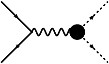
At LO in the HEFT, the tree-level amplitudes of the quark-antiquark subprocesses (thus, not including any form factor yet), are given, in their center of mass (CM), by
| (7) | |||||
| (8) | |||||
| (9) | |||||
| (10) | |||||
| (11) | |||||
| (12) |
where the and and (anti) quark subindices denote their helicity state and is the first parameter of the function appearing in the SISBS Lagrangian of Eq. (1): (notice that in the SM , ; a separation thereof signals strong interactions). Furthermore, and are respectively the sine and cosine of the Weinberg angle and
| (13) | |||||
Finally and are the energies of the produced and gauge bosons and and are the corresponding polar and azimuthal CM scattering angles, respectively.
At the high energies in which we are interested here , those amplitudes become:
| (14) | |||||
| (15) | |||||
| (16) | |||||
| (17) | |||||
| (18) | |||||
| (19) |
Guided by the precision LEP observables, we assume that custodial symmetry is a good approximation to the electroweak SISBS. This is obtained in the limit (which implies , so that and ). As experimentally , we will take . In the following we will simplify the amplitudes of Eq. (14) with that approximation. Then the non-vanishing ones are given by the simpler formulae
| (20) | |||||
| (21) |
whereas, because , .
In the presence of strong final state interactions, the amplitudes need to be modified by the introduction of an axial form factor . Thus the complete results will have the form
| (22) |
The nonperturbative computation is thus isolated into computing the form factor . Next, in section 4 we study in detail the and interactions and show how axial resonances arise out of these interactions.
4 The strongly interacting and amplitudes
In order to obtain the axial form factor that dresses the amplitudes in Eq. (20) one needs to have at hand an appropriate and as general as possible a description of elastic and scattering. Our approach here will start from the effective Electroweak Chiral Lagrangian in Eqs. (1) and (5). Then we will use the Equivalence Theorem [1] as applied to this kind of Lagrangian [2]. The theorem relates the electroweak amplitudes (in renormalizable gauges) involving longitudinal components of the and gauge bosons with the ones involving the corresponding would-be Goldstone bosons at high energies. In the case of interest here it reads (in the CM rest frame)
| (23) |
Therefore at high energies we can have access to the strongly interacting SBS of the SM by studying the elastic scattering of the longitudinal components of the , and the Higgs boson . While the gauge boson polarization is not yet systematically reconstructed at the LHC, it appears that it will soon become possible [18, 19].
The amplitude for the would-be Goldstone (’s) bosons and can be computed at tree level from the Lagrangian in Eq. (1) (order ). As this Lagrangian is not renormalizable, going to the one-loop level (oder ) requires the introduction of derivative counterterms depending on new couplings, as is standard in chiral perturbation theory. Upon renormalization, these couplings absorb the one-loop divergences of the elastic amplitudes and pararametrize, in a systematic way, our ignorance about the underlying SISBS for these processes. Thus, up to NLO, the relevant scalar Lagrangian in spherical coordinates is
| (24) | |||||
that we have described in detail in [20]. With this practical Lagrangian at hand we have computed the one-loop amplitudes for elastic processes involving Goldstone bosons and the Higgs. In the present application we provide the amplitude given by
| (25) |
where is the custodial isospin and , and are the standard Mandelstam variables for massless particles since at high energies we will be neglecting the Higgs (and vector boson) mass in agreement with Eq. (23). Then we obtain
| (26) | |||||
This can be obtained from our previously published [15, 16, 20] amplitude by crossing. The renormalized couplings and depend on the renormalization scale as
| (27) |
so that the amplitude in Eq. (26) is invariant.
If a resonance of definite spin appears dynamically or couples to in any way, it should appear in the corresponding partial wave amplitudes. It is then convenient to compute the first few partial waves that dominate the amplitude of Eq. (26) at low energy. The partial wave needed for this work is given by
| (28) |
where and . A direct computation of the integral shows that this partial wave adopts the generic form common to other scattering processes at NLO [14]:
| (29) |
where
| (30) | |||||
This axial-vector partial wave is defined in the whole complex plane and it has the expected left cut (LC) along the negative real -axis and the unitarity or right cut (RC) along the positive real -axis. The physical amplitude is obtained by taking , i.e. just over the RC, with being the total CM energy.
At low energies, phase space for channels with more particles suppresses inelastic amplitudes and elastic unitarity on the physical region is rather well satisfied, so that
| (31) |
However the NLO amplitude in Eq. (29) fulfills the unitarity condition at a perturbative level only,
| (32) |
This is equivalent to the relation among the constants of Eq. (30), which can be very easily checked. The more demanding exact elastic unitarity condition of Eq. (31) can be satisfied, with only the NLO computation at hand, by using, among other possibilities [20], the Inverse Amplitude Method (IAM [21]). According to it, the unitarized amplitude is given by
| (33) |
This amplitude fulfills the exact elastic unitarity condition in Eq. (31), it has the proper analytical structure (LC and RC), it is -independent and its low-energy expansion coincides with the HEFT up to the NLO:
| (34) |
Moreover, for certain regions of the coupling space, this amplitude (33) can feature a pole at some point in the second Riemann sheet of the complex plane. Any such poles have a natural interpretation as dynamically generated resonances with mass and width given by the relation . The IAM method has been extensively and successfully applied to ordinary Chiral Perturbation Theory to describe pion and kaon scattering and the associated resonances , and many others. Thus we may have some confidence that the method could work also in reproducing dynamical resonances in the context of the SISBS of the SM.
Since the IAM formula is compact and simply algebraic, as opposed to the difficult integral expressions of usual dispersion relations, we can study the position of its complex -plane poles (resonances) directly. In the case of axial resonances with mass and relative small width (so that ) we find
| (35) | |||||
| (36) |
where
| (37) |
and the and couplings are evaluated at (it is necessary to state this since is not, in general, renormalization-scale invariant). Obviously the region of parameters , , and yielding a dynamical axial resonance is defined as the region (though below about 500 GeV our use of the Equivalence Theorem does not hold scrutiny anymore) and .
Equation (35) shows that the LO parameters alone (that is, but ) are sufficient to generate an axial resonance. This is generically broad, as the width is proportional to the same separation from the SM. In the limit fulfilled by dilatonic theories [22] and the SM, the axial-vector becomes narrow, , and gets a mass , implying . Likewise, one gets the lower bound TeV for . In the SM (), this mass goes to infinity, decoupling from the low-energy theory. Such resonances are generically called “dynamically generated” and it is unclear whether they correspond to a new particle or field that should enter a fundamental Lagrangian, depending on how broad the width is. The textbook example of this behavior is the or -meson in hadron physics.
On the other hand, the NLO coefficients or can yield a light resonance, as they suppress the numerator in Eq.(35). The resonance is then narrower, as Eq. (37) shows a kind of KSFR relation: the width is proportional to the cube of the mass times a known combination of the coefficients that does not depend on , . Very often one expects that a resonance dominated by the NLO Lagrangian terms is actually a physical particle, and there is ample work integrating out that high energy field from the underlying action to yield expressions for the EFT coefficients in terms of its properties.
Figures 2, 3 and 4 illustrate the resonances obtained in various cases of interest, depending on the Lagrangian parameters. These amplitudes only depend on the combination , so have fixed and varied in all the plots.


The method can accommodate a variety of resonances (or none). Nevertheless, being based on an underlying Lagrangian, once its parameters are measured it does have predictive power yielding a specific spectrum and scattering amplitudes at higher energies.
5 The axial-vector form factor up to NLO in HEFT
The piece connecting the Strongly Interacting Sector described in section 4 with its perturbative coupling to the fermions of the Standard Model as in section 3 is the axial form factor in the sector that dresses the reaction. In this section we quickly compute it in perturbation theory, and defer the more sophisticated treatment necessary to address resonances for the next section.
In our treatment of the low-energy HEFT, the necessary operators at lowest order are provided by Eq. (1) and those at next-to-leading order by Eq. (5). In particular, in the ET limit the Axial Form Factor (AFF) only depends on one NLO effective coupling, . At NLO in this limit this operator absorbs the ultraviolet divergences cause by the one-lop AFF diagrams built out of the LO vertices from (1). In respecting custodial symmetry, the neutral-current form factor is provided by an isospin rotation and coincides with the charged one.
The computation of the AFF proceeds by extracting the kinematic factors from the matrix element
| (38) |
with , in the timelike region for our application, and the charged current being (with in the SM). In practice this means that the vertex function for with external on-shell and (but off-shell) is equal to
| (39) |
The normalization of the AFF defined in Eq. (38) at zero momentum transfer is , in consistency with the definition employed in previous sections. To achieve this, a factor has been explicitly factorized out (other works [23, 24] include this factor within instead).
Within the ET and neglecting once more the Higgs and W and Z masses at energies high enough over the threshold one obtains the low-energy effective theory prediction for the AFF up to NLO,
| (40) |
where
| (41) |
in a notation analogous to Eq. (29)
| (42) |
The NLO effective coupling renormalizes the one–loop divergence (here in the scheme in dimensional regularization) and runs with the scale in the form
| (43) |
such that is independent and in agreement with the path integral renormalization in [25] (with notation therein).
The EFT result from Eq. (41) and (42) does not depend on whether the Goldstone field is parametrized in spherical, exponential, or any other coordinates. This satisfying feature happens, in the () approximation because the four LO vertices active in the computation (, , and ) and the one NLO vertex () all have at most two Goldstone fields each.
The AFF from Eq. (41) and (42) is an analytical function in the whole complex -plane but for a RC, as expected. On the other hand, in the elastic regime, unitarity relates the imaginary part of the axial form factor with the partial-wave scattering amplitude in the form
| (44) |
However the one-loop result only fulfills this relation at the perturbative level -i.e., up to NLO in the low-energy expansion–:
| (45) |
where on the last step we have used that and that the tree-level amplitude is real. This is easy to check comparing Eq. (42) and (30), which satisfy . The reason of the violation of (exact) unitarity in the EFT calculation is the absence of higher order corrections. As far as energies remain small enough this deviations are negligible and our effective theory provides an appropriate approximation of the physical amplitude.
6 The Axial Form Factor in the resonance region
In this section we address the problem of how to obtain an appropriate AFF to describe the and resonant production at the LHC. We deploy four different methods and show that, for relatively narrow resonances, all give very similar results.
6.1 AFF with a resonance Lagrangian
The simplest approach, often employed by experimental collaborations in the search for new particles, is to include the resonance field explicitly as a degree of freedom in the Lagrangian [13, 23]. At tree-level, one finds a Breit-Wigner like formula
| (46) | |||||
where the and constants are respectively the and vertex couplings; in the last identity, they are [13, 23] fixed by
| (47) |
upon demanding that the AFF vanishes at asymptotically high energy (this depends on the underlying theory, and is typical, for example, of a non-Abelian gauge Lagrangian which yields asymptotic freedom).
Expanding the AFF (46) in powers of the squared four-momentum one obtains the tree-level matching condition , in agreement with previous works [13].
The intermediate resonance need not be infinitesimally narrow and its width can be taken into account easily (which makes the form-factor regular on the real axis), yielding the relativistic Breit-Wigner line shape,
| (48) |
In principle is an independent parameter. Nevertheless, if the presumed resonance is very elastic, suppressing other decay channels, the coupling of the resonance Lagrangian governs the width directly via
| (49) |
where the coupling is expected to be of .
Adding the experimental constraints from the oblique and parameters, further reduces the number of parameters. For instance, under the assumption that the correlator obeys two Weinberg sum-rules dominated by the lightest vector and axial-vector resonances [23], the axial-vector width becomes
| (50) |
Thus, for instance, a TeV resonance would have a width GeV for . A noticeable feature of Eq. (50) is the absence of the ubiquitous factor –compare it, for example, with Eq. (37)–. The reason is that the underlying effective Lagrangian including resonances explicitly correlates and , so there is one less parameter.
Obviously, in less constrained scenarios where some of the previous theoretical assumptions are relaxed, one could obtain broader resonances. But masses of a few TeV and widths of a few hundred GeV naturally appear in HEFT frameworks if the underlying theory is taken to be QCD-like.
In the next subsection 6.2, we avoid introducing the resonance as an explicit degree of freedom affecting and instead study it from analyticity and unitarization of the low-energy HEFT amplitude.
6.2 Unitarized HEFT parametrizations of the Axial Form Factor
Ideally, a fully realistic axial form factor would have the following properties:
- a
Analiticity in the complex plane, featuring just a right cut for physical . (We already know empirically that there are no bound state poles below threshold in the 100-Gev spectrum).
- b
Coincidence of any resonance poles (in the second Riemann sheet) with those of the elastic amplitude .
- c
- d
Low-energy behavior that reproduces the chiral expansion .
Model I in Eq. (48) features a resonance as in (b) and can be matched to the low-energy expansion (d), but has no cut and bears no ressemblance to the elastic amplitude, so that (a), (c) and most of (b) fail to be satisfied.
An alternative [26] would be to build a form factor from a Lippman-Schwinger like resummation of the perturbative form factor expansion,
| (51) | |||||
which inherits from the correct right cut, satisfying (a) and, by construction, (d), but is again unconnected to the elastic amplitude, so it fails to fulfill (b) and (c).
From the elastic amplitude alone it is possible to build another form factor model [27, 28] that satisfies (b) and (c)
| (52) | |||||
but, having no knowledge of , which is in principle independent, fails (d); and since has a left cut, it fails also (a) (while this feature is probably not severe if employed in the resonance region only, from which that spurious left cut is very far in the complex -plane).
One can improve Eq. (52) by correcting for the low energy expansion, introducing as follows,
| (53) |
This form factor satisfies all of (b), (c) and (d). The only problem left is that, together with the RC, it has also a LC from . But again, this LC is not expected to have a very strong influence in the physical timelike- region (the RC) particularly in the TeV, perhaps resonant, range of energies.
Interestingly, all three form factors in models II-IV, Eq. (51), (52), (53) would coincide if . This boils down to the following relations among the coefficients of and those of ,
| (54) | |||||
| (55) | |||||
| (56) |
The first condition is equivalent to neglecting the LC contribution and it is fulfilled for (as in the SM) or . The second identity is always obeyed, since it is a consequence of perturbative unitarity. The last one imposes a relation between and the rest of the couplings so it can be fulfilled by a proper election of this parameter as a function of those in the Lagrangian of Eq. (5), namely and the combination .
In general this choice of the parameter appears to be possible only at a given scale, so it would be dependent; however, if Eqs. (54) and (55) are obeyed then the right-hand and left-hand sides of Eq. (56) have exactly the same running and all choices of are equivalent; the appropriate choice of is
| (57) |

| Model | Eq. in text | Parameters | |
|---|---|---|---|
| I | ( Breit-Wigner like) | (48) | |
| II | (Lipmann-Schwinger on pert. FF) | (51) | |
| III | (From elastic IAM only) | (52) | |
| IV | (Combined pert. FF + IAM) | (53) |
In figure 5 we plot all four factor models for a relatively narrow resonance in the neighbourhood of 3 TeV (this is achieved by appropriately setting either or , depending on the model, see table 1). The agreement among them is spectacular (a consequence of the resonance being relatively narrow, so that the amplitude is pole-dominated) and therefore, it does not really matter what form factor model is used.
If one wants a quick cross-section estimate, the Breit-Wigner model (I) can as well be used; to use experimental data to constrain low-energy parameters of HEFT, the others should be implemented.
7 Cross section from intermediate gauge boson production
Now we are in a condition to provide a quick estimate for the resonant production of and at the LHC. After this extensive discussion, all pieces that enter the cross-section are at hand. For example we have, for the unpolarized CM cross-section,
| (58) | |||||
Integrating over the full solid angle, one obtains
| (59) |
The strongly interacting SBS dynamics is encoded in the form factor which can be resonant or not depending on the parameters of the effective Lagrangian. If is conserved by the SISBS (as in our HEFT calculation up to NLO), the same formula provides . Likewise, the production cross section is given by Eqs. (58) and (59) times a multiplicative factor , and multiplied by the appropriate distribution functions and summed on for the production from collisions.
Convoluting Eq. (59) with the parton distribution functions (which we take from the CJ (CTEQ-Jefferson Laboratory) set [29], that includes nuclear corrections, important at high and thus at the energy frontier of the LHC, as well as corrections), we obtain the proton-proton level inclusive cross-section to produce a or pair (by using the corresponding amplitudes given above) as:
with and . Here, is the CM squared energy of the pair, while is the CM energy of the LHC accelerator. A similar expression can be derived for the production, which provides a cross section of a similar order of magnitude and will not be studied in this exploratory work. For the example cross-section plotted in fig. 6, we have set at 13 TeV. There, a resonance of mass 3 TeV and width 0.4 TeV has been injected with two of the form factors from fig. 5. The LO parameters are , (away from their SM values ), and the NLO ones and for TeV. 33 3 This , which leads to TeV and TeV, is very close to the value one would obtain from through (57), . The proximity of this two values relies on the fact that both expressions lead to the same resonance pole and the conditions from (54)–(56) for BSM theories, , is approximately fulfilled by our benchmark point .


Since the resonances here analyzed are native of the EW SBS, they are rather elastic and the branching fraction is not too far below 1 and the difference therefrom can be ignored in a first experimental analysis (unlike other types of new physics that are weakly coupled to this channel).
We do find small cross-sections (fractions of a femtobarn) that are well below the current CMS and ATLAS cross-section upper bounds. The experimental collaborations are constraining and models where the new resonance couples directly with charges and , leading to femtobarn-size cross-sections. On the other hand, our computations proceed by the diagram of fig. (1) with an intermediate gauge boson and are smaller by a factor . This means that it will be arduous for the LHC to fully constrain the “natural” parameter space in the 3 TeV region. For this reason, we look forward to its high-luminosity upgrade.
8 Conclusions
The IAM has been applied in this article to describe the strong elastic rescattering in the regime where the ET applies () that is, for energies above about 500 GeV, and, at the same time, an EFT description in terms of the low energy degrees of freedom makes sense (, with the vev scale of spontaneous symmetry breaking in the strong BSM sector).
Notice again that we are neglecting masses and CKM mixing for this exploratory study. Clearly, a more exhaustive analysis should take into account the detector acceptance and appropriate kinematical cuts in the angular integration. Likewise, the and are not directly detected, but rather their decay products. Nevertheless, this type of ‘realistic’ analysis is out of the scope of this article and is relegated to future studies.
If the precision program of the LHC measures deviations from the SM in the low energy coefficients of the chiral Lagrangian (the relevant combinations of , , and for this work) EFT-based approaches can predict whether there is new physics within reach of the LHC. These methods are sufficiently robust to qualitatively predict whether there is a reasonable hope of detecting new physics resonances within the accelerator’s energy reach, through equation (35). In our case, the axial-vector resonance mass and width and the low-energy parameters are constrained through the KSFR-like relation in Eq. (37).
If other unitarization methods such as the N/D or the (improved) K-matrix method are employed, the results are consistent, and the theoretical method-choice uncertainty is about 20% in the determination of the resonance mass, as it was recently shown in [20]. One generically expects this from any unitarization method that respects analyticity in the complex plane. To reproduce an analytic function in its entire domain of analyticity (for example, a scattering amplitude in the resonance region) it is enough to know it with enough precision in a finite segment (for example, where the LHC can measure the low-energy coefficients) and to provide an appropriate analytical extension. Thus, unitary and analytic methods do have some predictive power. On the contrary, methods such as the old K-matrix are unitary but lack the right analytic structure, being less reliable.
Finally, it is worth remarking that our strongly interacting SBS analysis with chiral NLO couplings ( and here) of the order of leads to much smaller production cross sections than those currently tested by ATLAS and CMS [30]. This naturally allows the presence of resonances with mass TeV, while evading standing experimental bounds in resonant production, contrary to some of the theoretical models considered by the experimental collaborations.
Acknowledgments
The authors thank Rafael L. Delgado for assistance and valuable comments at early stages of this investigation. We also want to thank M.J. Herrero and D. Espriu for useful comments and suggestions, and the members of UPARCOS for maintaining a stimulating intellectual atmosphere. Work supported by Spanish grants MINECO:FPA2014-53375-C2-1-P, FPA2016-75654-C2-1-P and the COST Action CA16108.
References
- [1] J. M. Cornwall, D. N. Levin and G. Tiktopoulos, Phys. Rev. D 10 (1974) 1145 Erratum: [Phys. Rev. D 11 (1975) 972]. doi:10.1103/PhysRevD.10.1145, 10.1103/PhysRevD.11.972; C. E. Vayonakis, Lett. Nuovo Cim. 17 (1976) 383. doi:10.1007/BF02746538 B. W. Lee, C. Quigg and H. B. Thacker, Phys. Rev. D 16 (1977) 1519. doi:10.1103/PhysRevD.16.1519; M. S. Chanowitz and M. K. Gaillard, Nucl. Phys. B 261 (1985) 379. doi:10.1016/0550-3213(85)90580-2; G. J. Gounaris, R. Kogerler and H. Neufeld, Phys. Rev. D 34 (1986) 3257. doi:10.1103/PhysRevD.34.3257.
- [2] A. Dobado and J. R. Peláez, Nucl. Phys. B 425 (1994) 110 Erratum: [Nucl. Phys. B 434 (1995) 475] doi:10.1016/0550-3213(94)90174-0, 10.1016/0550-3213(94)00533-K [hep-ph/9401202]; Phys. Lett. B 329 (1994) 469 Addendum: [Phys. Lett. B 335 (1994) 554] doi:10.1016/0370-2693(94)90392-1, 10.1016/0370-2693(94)91092-8 [hep-ph/9404239]; C. Grosse-Knetter and I. Kuss, Z. Phys. C 66 (1995) 95 doi:10.1007/BF01496584 [hep-ph/9403291]; H. J. He, Y. P. Kuang and X. y. Li, Phys. Lett. B 329 (1994) 278 doi:10.1016/0370-2693(94)90772-2 [hep-ph/9403283].
- [3] D. de Florian et al. [LHC Higgs Cross Section Working Group], doi:10.23731/CYRM-2017-002 arXiv:1610.07922 [hep-ph].
- [4] J. J. Sanz-Cillero, arXiv:1710.07611 [hep-ph].
- [5] A. Castillo, R. L. Delgado, A. Dobado and F. J. Llanes-Estrada, Eur. Phys. J. C 77, no. 7, 436 (2017) doi:10.1140/epjc/s10052-017-4991-6 [arXiv:1607.01158 [hep-ph]].
- [6] R. L. Delgado, A. Dobado, D. Espriu, C. Garcia-Garcia, M. J. Herrero, X. Marcano and J. J. Sanz-Cillero, arXiv:1707.04580 [hep-ph].
- [7] F. Feruglio, Int. J. Mod. Phys. A 8 (1993) 4937; R. Alonso et al., Phys. Lett. B 722 (2013) 330 Erratum: [Phys. Lett. B 726 (2013) 926]; G. Buchalla, O. Catà and C. Krause, Nucl. Phys. B 880 (2014) 552 Erratum: [Nucl. Phys. B 913 (2016) 475].
- [8] S. R. Coleman, J. Wess and B. Zumino, Phys. Rev. 177 (1969) 2239. doi:10.1103/PhysRev.177.2239; C. G. Callan, Jr., S. R. Coleman, J. Wess and B. Zumino, Phys. Rev. 177 (1969) 2247. doi:10.1103/PhysRev.177.2247.
- [9] T. Appelquist and C. W. Bernard, Phys. Rev. D 22 (1980) 200; A. C. Longhitano, Phys. Rev. D 22 (1980) 1166; Nucl. Phys. B 188 (1981) 118.
- [10] The ATLAS collaboration [ATLAS Collaboration], ATLAS-CONF-2017-018.
- [11] A. M. Sirunyan et al. [CMS Collaboration], arXiv:1707.01303 [hep-ex]; H. Huang, on behalf of the CMS coll., arXiv:1710.05230 [hep-ex]; A. M. Sirunyan et al. [CMS Collaboration], Phys. Lett. B 774, 533 (2017) doi:10.1016/j.physletb.2017.09.083 [arXiv:1705.09171 [hep-ex]].
- [12] A. Pich, I. Rosell, J. Santos and J. J. Sanz-Cillero, Phys. Rev. D 93 (2016) no.5, 055041 doi:10.1103/PhysRevD.93.055041 [arXiv:1510.03114 [hep-ph]].
- [13] A. Pich, I. Rosell, J. Santos and J. J. Sanz-Cillero, JHEP 1704 (2017) 012 doi:10.1007/JHEP04(2017)012 [arXiv:1609.06659 [hep-ph]].
- [14] R. L. Delgado, A. Dobado and F. J. Llanes-Estrada, J. Phys. G 41 (2014) 025002 [arXiv:1308.1629 [hep-ph]].
- [15] R. L. Delgado, A. Dobado and F. J. Llanes-Estrada, JHEP 1402 (2014) 121 [arXiv:1311.5993 [hep-ph]].
- [16] R. L. Delgado, A. Dobado and F. J. Llanes-Estrada, Phys. Rev. Lett. 114, no. 22, 221803 (2015) doi:10.1103/PhysRevLett.114.221803 [arXiv:1408.1193 [hep-ph]].
- [17] G. Aad et al. [ATLAS and CMS Collaborations], JHEP 1608, 045 (2016) doi:10.1007/JHEP08(2016)045 [arXiv:1606.02266 [hep-ex]].
- [18] J. A. Aguilar-Saavedra, J. Bernabéu, V. A. Mitsou and A. Segarra, Eur. Phys. J. C 77, no. 4, 234 (2017) doi:10.1140/epjc/s10052-017-4795-8
- [19] E. Maina, contribution to the EPS-HEP international conference on high energy physics, Venice, July 6th 2017, https://indico.cern.ch/event/466934/contributions/2575374/
- [20] R. L. Delgado, A. Dobado and F. J. Llanes-Estrada, Phys. Rev. D 91, no. 7, 075017 (2015) [arXiv:1502.04841 [hep-ph]].
- [21] A. Dobado, M.J. Herrero and T.N. Truong, Phys. Lett. B235 (1990) 134; A. Dobado and J.R. Pelaez, Phys. Rev. D47 (1993) 4883; Phys. Rev. D 56 (1997) 3057.
- [22] E. Halyo, Mod. Phys. Lett. A 8 (1993) 275. doi:10.1142/S0217732393000271; W. D. Goldberger, B. Grinstein and W. Skiba, Phys. Rev. Lett. 100 (2008) 111802 doi:10.1103/PhysRevLett.100.111802 [arXiv:0708.1463 [hep-ph]].
- [23] A. Pich, I. Rosell and J. J. Sanz-Cillero, JHEP 1401 (2014) 157 doi:10.1007/JHEP01(2014)157 [arXiv:1310.3121 [hep-ph]].
- [24] A. Pich, I. Rosell and J. J. Sanz-Cillero, Phys. Rev. Lett. 110 (2013) 181801 doi:10.1103/PhysRevLett.110.181801 [arXiv:1212.6769 [hep-ph]].
- [25] F. K. Guo, P. Ruiz-Femenía and J. J. Sanz-Cillero, Phys. Rev. D 92 (2015) 074005 doi:10.1103/PhysRevD.92.074005 [arXiv:1506.04204 [hep-ph]].
- [26] T.N. Truong, Phys. Rev. Lett. 61 (1988) 2526.
- [27] A. Dobado, M. J. Herrero, J. R. Pelaez and E. Ruiz Morales, Phys. Rev. D 62, 055011 (2000) [hep-ph/9912224].
- [28] D. Espriu and F. Mescia, Phys. Rev. D 90, no. 1, 015035 (2014) [arXiv:1403.7386 [hep-ph]]. D. Espriu, F. Mescia and B. Yencho, Phys. Rev. D 88, 055002 (2013) [arXiv:1307.2400 [hep-ph]]. D. Espriu and B. Yencho, Phys. Rev. D 87, no. 5, 055017 (2013) [arXiv:1212.4158 [hep-ph]].
- [29] J. F. Owens, A. Accardi and W. Melnitchouk, Phys. Rev. D 87, no. 9, 094012 (2013) doi:10.1103/PhysRevD.87.094012 [arXiv:1212.1702 [hep-ph]].
- [30] G. Aad et al. [ATLAS Collaboration], arXiv:1506.00962 [hep-ex]; M. Aaboud et al. [ATLAS Collaboration], Phys. Lett. B 765, 32 (2017) doi:10.1016/j.physletb.2016.11.045 [arXiv:1607.05621 [hep-ex]].