YITP-17-126
IPMU17-0163
Renyi Entropy for Local Quenches in 2D CFTs
from Numerical Conformal Blocks
Yuya Kusukia and Tadashi Takayanagia,b
aCenter for Gravitational Physics,
Yukawa Institute for Theoretical Physics (YITP), Kyoto University,
Kitashirakawa Oiwakecho, Sakyo-ku, Kyoto 606-8502, Japan
bKavli Institute for the Physics and Mathematics of the Universe,
University of Tokyo, Kashiwano-ha, Kashiwa, Chiba 277-8582, Japan
We study the time evolution of Renyi entanglement entropy for locally excited states in two dimensional large central charge CFTs. It generically shows a logarithmical growth and we compute the coefficient of term. Our analysis covers the entire parameter regions with respect to the replica number and the conformal dimension of the primary operator which creates the excitation. We numerically analyse relevant vacuum conformal blocks by using Zamolodchikov’s recursion relation. We find that the behavior of the conformal blocks in two dimensional CFTs with a central charge , drastically changes when the dimensions of external primary states reach the value . In particular, when and , we find a new universal formula . Our numerical results also confirm existing analytical results using the HHLL approximation.
1 Introduction and Summary
One useful way to characterize dynamical aspects of quantum field theories (QFTs) is to study properties of entanglement entropy [1, 2, 3, 4, 5, 6, 7]. Especially, the evolutions of entanglement entropy when we excite QFTs provide us with important pieces of information such as whether the quantum field theory is integrable or chaotic. Indeed, this has been manifest for locally excited states in conformally field theories (CFTs) as we briefly review below.
A famous example in this direction is the studies of global quantum quenches, which are translationally invariant excited states created by a sudden change of the Hamiltonian [8] (also refer to references in [9]). The time evolution of entanglement entropy under global quenches shows a causal and relativistic propagation of elementary excitations in generic CFTs. One way to study how the details of propagations of quantum entanglement are different beyond this universal behavior is to look at local excitations rather than global excitations. Motivated by this, the main purpose of this paper is to study the time evolution of entanglement when we locally excite a class of CFTs which are strongly interacting and have many degrees of freedom. Such a class of CFTs have holographic duals and is called holographic CFTs [10, 11, 12].
A locally excited state (operator local quench) is defined by acting with a local operator on the CFT vacuum in the manner11 1 We would like to stress that in (1) is the UV cut off of the local excitations and should be distinguished from the UV cut off (i.e. the lattice spacing) of the CFT itself.
| (1) |
where is the normalization factor. The infinitesimally small parameter provides a UV regularization as the truly localized operator has infinite energy. Consider the time evolution of the entanglement entropy and more generally Renyi entanglement entropy for the time evolved excited state . We choose the subsystem to be the half-space and is the corresponding reduced density matrix. The excitation is originally located in the subsystem (i.e. complement of ), thus it creates additional entanglement between them. The main quantity of interest is the growth of entanglement entropy compared to the vacuum:
| (2) |
Note that the limit coincides with the von-Neumann entropy (or entanglement entropy) growth . If we define to be the distance between and the boundary point , for as follows from the causality. For , gets non-vanishing in general as the excitations in the region can reach the region .
Calculations of for massless scalar fields have been performed in [13, 14, 15, 16] and it was found that the growth approaches a finite positive constant at late time. This is clearly interpreted as a system of entangled particles propagating at the speed of light [17]. The same behavior has also been found for rational CFTs in two dimensions, which is a typical example of integrable CFTs, [14, 18, 19, 20, 21, 22].
Furthermore, a recent study of 1+1-dimensional orbifold CFTs found an exotic time evolution for irrational (but exactly solvable) CFTs [23]. For other field theoretic progress on local quenches refer also to [24, 25, 26, 27, 28, 29, 30, 31, 32, 33, 34].
On the other hand, for holographic CFTs, which are strongly interacting CFTs with large central charges [10, 11, 12], the evolution behavior changes drastically. In the calculation using the holographic formula [35, 36], the local excitation corresponds to a massive particle falling in AdS3, whose mass is related to the conformal dimension of in (1) via the standard relation ( is the AdS radius). The holographic results for the (von-Neumann) entanglement entropy under time evolution at late time was obtained in [37] and this reads
| (3) |
where is the central charge of the 2D holographic CFT.
This time dependence has been precisely reproduced in [38] using a large central charge CFT analysis. Such a behavior is expected to stem from the chaotic nature of holographic CFTs, where the quasi-particle picture breaks down. Similar calculations in higher dimensional holographic CFTs have recently performed in [39] for a holographic computation in the AdSCFT3 setup, where like behavior was observed.
In summary, the functional form of the growth of von-Neumann entanglement entropy depends on the nature of CFTs roughly in such a way that as interactions in the CFT get stronger, the rate of its growth increases. In [23], it was even conjectured that the logarithmic growth (3) found in the holographic 2d CFTs give an upper bound of the growth rate for any two dimensional CFTs. In this way, we already had enough knowledge about the von-Neumann entanglement entropy for the locally excited states.
However, to capture more information of quantum entanglement, we need to look at the Renyi entanglement entropies for various . At present, we have only limited understanding of for the locally excited states as we will briefly review below. To obtain the full understanding of the time evolutions of the Renyi entanglement entropies is the main purpose of the present paper.
For the Renyi entanglement entropy in 2D holographic CFTs, the following behavior was derived in [40] when the (chiral) conformal dimension of local operator is small enough: :
| (4) |
In this way, interestingly, there are varieties of behaviors of (Renyi) entanglement entropy for the locally excited states defined by (1), depending on how much a given CFT is chaotic. Notice that the above operator local quench makes a significant contrast with the original class of local quenches introduced in [41] (see also [42, 9]) defined by joining two semi-infinite CFTs, which always lead to logarithmic growth of entanglement entropy for any two dimensional CFTs, both integrable and chaotic.
In this paper, we would like to explore more on the analysis of for 2D holographic CFTs to obtain complete and systematic understandings without relying on special approximations. For example, one may notice that it is not immediately clear why the two results (3) for the von-Neumann entropy and (4) for the Renyi entropy with are related to each other. Indeed, the latter gets divergent in the von-Neumann limit . Moreover, there is no known result for the evolution of Renyi entropy with large .
To find a full control of the computability for any values of and we will employ the powerful numerical program recently developed in [43] by Chen, Hussong, Kaplan and Yi, based on Zamolodchikov’s recursion relation [44, 45, 46, 47]. For example, this relation was applied to computations of entanglement entropy for multi-intervals in [48]. This powerful and non-perturbative method allows us to evaluate any conformal blocks with any values of conformal dimensions and central charges . Note that for the replica computation of the Renyi entanglement entropy we set . Therefore in this paper we express the total (replicated) central charge as when we talk about the conformal blocks.

As we will explain later in the present paper, our analysis reveals that the behavior of conformal block changes drastically when the conformal dimensions are large. We find that the behavior of vacuum conformal block for the 4-pt function of the form can be classified into three regions , , and . The region is equivalent to . In region the coefficients of the power series of the function , which is an important part of the contributions to the conformal block, grows polynomially. On the other hand in the region and , grows exponentially.
In terms of our Renyi entanglement entropy calculations, these regions correspond to , , , and . In particular, studies of the region lead to the following new universal behavior of Renyi entropy growth
| (5) |
On the other hand, in the region and , we can apply the formula (3) when , while in the region and we can apply the formula (4) when . These behaviors are summarized in Fig.1. It will be an intriguing future problem to reproduce the new behavior (5) from holographic calculations. Also it is an important to understand better the nature of the non-trivial transition of the conformal blocks at .
This paper is organized as follows: In section two, we review the computation of Renyi entanglement entropy in large central charge CFTs. In section three we analyse the vacuum conformal blocks by using the Zamolodchikov’s recursion relation for various parameter regions. In section four, we apply the results of section three to the computations of Renyi entanglement entropy. In appendix A we summarize our conventions of four point functions and conformal blocks. In appendix B we briefly review the Zamolodchikov’s recursion relation .
2 Renyi Entropy and Conformal Blocks
Here we review the general calculation of Renyi entanglement entropy for excited states in a 2D CFT in terms of conformal blocks. We express the 2D CFT we consider as and its central charge is written as .
2.1 Growth of Renyi Entropy for Excited States
In the replica computation for Renyi entropy we introduce the replicated CFT with the central charge . The growth of Renyi entropy (2) for locally excite states (1) can be expressed by [49, 38]
| (6) |
we take the subsystem to be a semi-infinite interval and the twist operators are inserted at both end points of . Here is defined on the cyclic orbfold CFT (replicated CFT) (with the central charge ), using the operators in the seed CFT (with the central charge ) as
| (7) |
which is separated by the distance from the boundary of as shown in Fig.2. We take the subsystem to be the half line . In the complex plane , we insert the two twist operators each at and . The replicated operator , which produces the state of the local excitation, is inserted at and the other, which creates , is at as in Fig.2. The rule of the analytical continuation from the Euclidean time to Lorentzian time follows from the prescription in [8]. Now, these insertions of four operators lead to the growth of the trace of the reduced density matrix i.e. that of Renyi entropy as in (6).
We define the chiral conformal dimension of as . Then the dimension of is written as . The dimension of twist operator is given by the standard formula
| (8) |

By using the cross ratio , we can rewrite (6) as
| (9) |
where is the four point function (refer to appendix A for more details of our conventions)
| (10) |
and the cross ratio is explicitly expressed as
| (11) |

From these expressions, one find that the sign of the imaginary part of the cross ratio changes at . As a result, the cross ratio picks up the factor at as (see Fig.3). This does not happen for the anti-chiral coordinate . We write the value of after this monodromy transformation as . For example, if , then . In the late time region , which we are interested in, we find
| (12) |
Therefore the time evolution of excited Renyi entropy at late time can be calculated as
| (13) |
The 4-pt function can be expressed as a summation over conformal blocks . In holographic CFTs we expect that due to its sparse spectrum, we can approximate by restricting to the vacuum conformal block . Thus we obtain
| (14) | |||||
This is the main target which we would like to evaluate in this paper.
3 Analysis of Conformal Blocks
In this section, after we review the numerical computation of conformal block based on Zamolodchikov’s recursion relation, we explore properties of conformal block towards the calculation of Renyi entropy. We are especially interested in large central charge limit .
3.1 Conformal Blocks and Numerical Approach
As in [44], the conformal block for the 4-pt function can be expressed in the following way ( is the dimension of intermediate primary):
| (15) |
where
| (16) |
and
| (17) |
It is useful to note and when is small we have . We can express in terms of the theta functions as .
The function is found by solving the recursion relation in [44], whose numerical prescription was formulated in [43] (see appendix B of this paper). It is expanded as
| (18) |
It is important to note that has the symmetry:
| (19) |
This follows from the relation (61) for the full 4-pt function is true for each conformal block. This relation is expected because it just flips with and does not change the structure of channel.
One useful limit we take is . Accordingly approaches to . We write this as with . Then we have in this limit:
| (20) |
3.2 Simplest Example of : Vacuum Primary
If we consider the trivial limit of vacuum primaries , obviously we have . This fixes the form of as follows
| (21) | |||||
When is small (or equally is small), this is expanded as follows:
| (22) |
On the other hand, if we take the limit with , we find
| (23) |
where means the approximation up to a constant factor.
By using the approximation formula of a summation (based on the saddle point approximation) (we assume ):
| (24) |
When , we have
| (25) |
3.3 Behaviors of
Now we would like to examine the properties of for general and . We focus on the vacuum conformal block as that is relevant for our later calculations of Renyi entropy. First we can analytically calculate the coefficient assuming the large limit from the recursion relation:
| (28) |
However note that here we ignored the lower powers of and this approximation is only sensible for .
From this expression we find the following behavior of signs of (refer to Fig.4):
| (29) | |||||
| (30) | |||||
| (31) |
We summarized these behavior in Fig.5. Note that is invariant under the exchange of and as follows from the symmetry (19).


Now we perform numerical computations of employing the computer program made in the paper [43] (for a short summary, see also appendix B of the present paper). First, our numerical calculations of for various values of precisely show the above behaviors of signs, even for the regions . By fitting the numerical result for (refer to the plots Fig.6) in the Cardy formula-like form
| (32) |
and we evaluated the values of and for various and plotted in Fig.7.

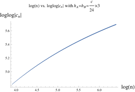
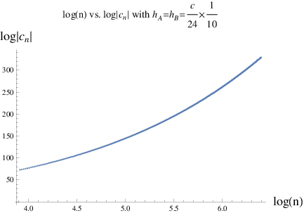
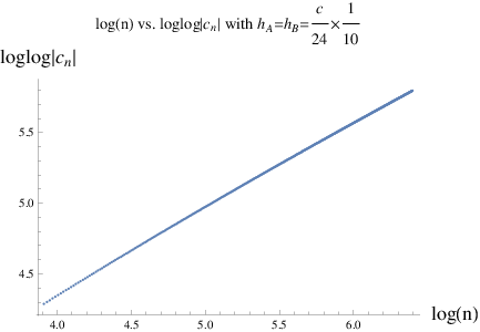
Interestingly we observe a clear transition of the values of and along the lines and as can be seen from the plots in Fig.7. This behavior is summarized as follows22 2 In the paper [43], it was argued that the power law like behavior in the limit can be observed for HHLL conformal block. Our analysis shows that this power law behavior (i.e. ) can only be seen for the region (i) and not in the region (ii) and (iii).
| (33) |
Here the functions and are smooth monotonic functions bounded as and . We have
| (34) | |||
| (35) | |||
| (36) |
Note that in (34) following from (27). As we will show in the next subsections, we can evaluate and by using the heavy-heavy-light-light (HHLL) approximation of conformal blocks assuming and . This leads to
| (37) | |||
| (38) |
Indeed, we find , which justifies (35) and shows that is continuous at the border between (ii) and (iii). The value of is found as
| (39) |
which can be applicable to both and if is small enough.
On the other hand, we would like to note that the result in the region , is well fitted with the numerical data by the formula first considered in [43]:
| (40) |
Note that the doubled coefficient of compared with (39) can be understood from the factor two difference of the power of between the formula (24) and formula (25).


3.4 HHLL Approximation
3.5 limit
When we consider the region i.e. , we need to worry about the alternating signs in (30), as behaves like . In such a case, it is not straightforward to obtain a formula like (24).
To cancel the signs, we consider another limit of . This is obtained by limit with a monodoromy transformation around . Explicitly we have
| (44) |
This behaves like (we define ):
| (45) |
From the HHLL approximation (41), we obtain the following behavior for the modular limit
| (46) |
By using the formula (24), we can read off from this behavior the advertised values of and given by (37) and (39).
Actually, this limit exactly corresponds to the one we need to calculate the Renyi entropy described in (12) i.e. . In this relation, we can identify .
4 Evaluation of Renyi Entropy
Now we are in a position to study the Renyi entropy computed by the formula (14) based on our previous results for the vacuum conformal block. First note that to calculate the -th Renyi entropy for a large central charge CFT (holographic CFT) with a central charge by the replica method, we consider a CFT with the central charge , defined by taking copies of the original CFT. Then we take
| (47) |
The growth of Renyi entropy is symmetric under the exchange of and as
| . | (48) |
Since we act the monodromy transformation only for and not for , in the limit (12) we have as in (45) and .
Thus we can simply (14) as follows
| (49) |
where we neglect subleading terms and keep such terms grow as in the end.33 3 In other words, we neglect terms .
In general, we find that grows logarithmically under time evolutions. Therefore, below, we are interested in the coefficient of the log term, denoted by :
| (50) |
The behaviors of are summarized in Fig.1. Our numerical results of are plotted in Fig.8 as we will explain below.


4.1 HHLL Approximation
If we apply the HHLL approximation with , we obtain from (46)
| (51) |
If we choose the light operator to be the twist operator in the limit , then we reproduce the formula (3). If we choose the light operator to be , namely the operator for the excitation, then we reproduce another formula (4). Note that these approximated results are continuous at . The regions where we can apply this HHLL approximation is depicted in Fig.1 as the red and green regions.
4.2 Region
In the region defined by (29), we simply have
| (52) |
namely the advertised formula (5). This is derived as follows. First note that does not give any leading divergence which contributes to entropy, remembering the behavior (i.e. no factor). Then the formula (49) with leads to the formula (52). Indeed this behavior is confirmed in the left plot in Fig.8.
4.3 Region
In the region (ii) defined by (30), we can apply the formula (24) in limit as we have explained in the previous section. Thus we can calculate the coefficient in (50) in terms of :
| (53) |
This function interpolates the HHLL approximated result and the formula (52) in the region . Examples of the plots of in this region can be found from the both two plots in Fig.8.
4.4 Region
The region (iii), defined by (31) also includes parameter spaces where we can apply the HHLL approximation. Also when and , we should reproduce the behavior (52). Even though we do not have any analytical formula, our numerical results show that the function monotonically interpolates these boundary values, as depicted in the right plot of Fig.8.
4.5 Comment on OTOC
In this paper, we focus on entropy, but the vacuum block we derived can be also used to evaluate OTOC. As in [54], we can express the late time behavior of OTOC in holographic CFTs as
| (54) |
The cross ratio is given by
| (55) |
where and is the separation between operators that keeps the ratio fixed. This technique is very similar to that used to calculate entropy. Therefore we can apply our result to calculating OTOC straightforwardly and it leads to the late time behavior of OTOC for any two operators, in particular two heavy operators. The result is as follows.
| (56) |
and in the heavy-light limit, we can reproduce the results in [54, 55]. Moreover we can conclude that the behaviors of OTOC show the late exponential decay for any operator at late time. This exponential decay cannot be seen in non-chaotic CFTs, where the OTOC approaches non-zero constant[56, 57] or decays polynomially [58]. This may suggest that this late time behavior can also be used as a criterion of chaotic nature of a given quantum field theory, in addition to the existing arguments on the Lyapunov exponent [54, 59, 60]. It is also intriguing to note that the above exponential decay behavior of OTOC is directly related to the logarithmic growth of Renyi entanglement entropy (5).
Acknowledgments
We thank Arpan Bhattacharrya, Kanato Goto, Yasuaki Hikida, Fabio Novaes, Shinsei Ryu, and Tomonori Ugajin for useful discussions, and in particular Pawel Caputa and Jared Kaplan for reading the draft of this paper and giving us valuable comments. TT is supported by the Simons Foundation through the “It from Qubit” collaboration. TT is supported by JSPS Grant-in-Aid for Scientific Research (A) No.16H02182. TT is also supported by World Premier International Research Center Initiative (WPI Initiative) from the Japan Ministry of Education, Culture, Sports, Science and Technology (MEXT). YK and TT are very grateful to the workshop “Holography and Dynamics” (YITP-X-17-06), held in Yukawa Institute for Theoretical Physics, Kyoto University where results of this paper were presented.
Appendix A Convention of 4-pt Function
Here we summarize our conventions on 4-pt functions and conformal blocks. Consider two kinds of primary operators with the dimension and with the dimension . The full expression of 4-pt function, written as , takes the following form
| (57) |
where is the cross ratio.
We define the (normalized) 4-pt function by taking the limit and by absorbing the divergence as follows:
| (58) |
In other words we find the relation
| (59) | |||||
On the other hand if we take the limit , we can define as follows:
| (60) |
By comparing (58) and (60) based on the expression (57), we find the relation
| (61) |
This relation is very natural because it is just an exchange of two s with two s.
The (normalized) 4-pt function can be written as the summation over all conformal blocks:
| (62) |
where is the conformal dimension of the intermediate primary state.
Appendix B Recursion Relations
In this Appendix, we will review Zamolodchikov’s recursion relation. In our case and , the Virasoro conformal block can be expressed as
| (63) |
and is given by the following recursion relation,
where is a zero of the Kac determinant and
| (67) |
Here the integers are defined as
| (68) |
The product in (67) means that we exclude and . We also defined
| (69) |
We expand as
| (70) |
In the same way as (B), we can also calculate the coefficients recursively by the following relation,
| (71) |
where the sum is took over with held fixed, i.e. the sum means taking sum over . The coefficient can be also calculated recursively by
| (72) |
where the starting values of this recursion formula are . Note that in this paper, we describe as .
References
- [1] L. Bombelli, R. K. Koul, J. Lee and R. D. Sorkin, “A Quantum Source of Entropy for Black Holes,” Phys. Rev. D 34 (1986) 373.
- [2] M. Srednicki, “Entropy and area,” Phys. Rev. Lett. 71 (1993) 666 [hep-th/9303048].
- [3] C. Holzhey, F. Larsen and F. Wilczek, “Geometric and renormalized entropy in conformal field theory,” Nucl. Phys. B 424 (1994) 443 [hep-th/9403108].
- [4] P. Calabrese and J. L. Cardy, “Entanglement entropy and quantum field theory,” J. Stat. Mech. 0406, P06002 (2004) [hep-th/0405152].
- [5] J. Bhattacharya, M. Nozaki, T. Takayanagi and T. Ugajin, “Thermodynamical Property of Entanglement Entropy for Excited States,” Phys. Rev. Lett. 110 (2013) no.9, 091602 [arXiv:1212.1164 [hep-th]].
- [6] D. D. Blanco, H. Casini, L. Y. Hung and R. C. Myers, “Relative Entropy and Holography,” JHEP 1308 (2013) 060 doi:10.1007/JHEP08(2013)060 [arXiv:1305.3182 [hep-th]].
- [7] G. Wong, I. Klich, L. A. Pando Zayas and D. Vaman, “Entanglement Temperature and Entanglement Entropy of Excited States,” JHEP 1312 (2013) 020 [arXiv:1305.3291 [hep-th]].
- [8] P. Calabrese and J. L. Cardy, “Evolution of entanglement entropy in one-dimensional systems,” J. Stat. Mech. 0504 (2005) P04010 doi:10.1088/1742-5468/2005/04/P04010 [cond-mat/0503393].
- [9] P. Calabrese and J. Cardy, “Quantum quenches in 1 + 1 dimensional conformal field theories,” J. Stat. Mech. 1606 (2016) no.6, 064003 doi:10.1088/1742-5468/2016/06/064003 [arXiv:1603.02889 [cond-mat.stat-mech]].
- [10] M. Headrick, “Entanglement Renyi entropies in holographic theories,” Phys. Rev. D 82 (2010) 126010 doi:10.1103/PhysRevD.82.126010 [arXiv:1006.0047 [hep-th]].
- [11] T. Hartman, “Entanglement Entropy at Large Central Charge,” arXiv:1303.6955 [hep-th];
- [12] T. Hartman, C. A. Keller and B. Stoica, “Universal Spectrum of 2d Conformal Field Theory in the Large c Limit,” JHEP 1409 (2014) 118 doi:10.1007/JHEP09(2014)118 [arXiv:1405.5137 [hep-th]].
- [13] M. Nozaki, T. Numasawa and T. Takayanagi, “Quantum Entanglement of Local Operators in Conformal Field Theories,” Phys. Rev. Lett. 112 (2014) 111602 doi:10.1103/PhysRevLett.112.111602 [arXiv:1401.0539 [hep-th]].
- [14] M. Nozaki, “Notes on Quantum Entanglement of Local Operators,” JHEP 1410 (2014) 147 doi:10.1007/JHEP10(2014)147 [arXiv:1405.5875 [hep-th]].
- [15] M. Nozaki, T. Numasawa and S. Matsuura, “Quantum Entanglement of Fermionic Local Operators,” JHEP 1602 (2016) 150 [arXiv:1507.04352 [hep-th]].
- [16] M. Nozaki and N. Watamura, “Quantum Entanglement of Locally Excited States in Maxwell Theory,” JHEP 1612 (2016) 069 [arXiv:1606.07076 [hep-th]].
- [17] M. Nozaki and N. Watamura, “Correspondence between Entanglement Growth and Probability Distribution of Quasi-Particles,” arXiv:1703.06589 [hep-th].
- [18] S. He, T. Numasawa, T. Takayanagi and K. Watanabe, “Quantum dimension as entanglement entropy in two dimensional conformal field theories,” Phys. Rev. D 90 (2014) no.4, 041701 doi:10.1103/PhysRevD.90.041701 [arXiv:1403.0702 [hep-th]].
- [19] B. Chen, W. Z. Guo, S. He and J. q. Wu, “Entanglement Entropy for Descendent Local Operators in 2D CFTs,” JHEP 1510 (2015) 173 [arXiv:1507.01157 [hep-th]].
- [20] P. Caputa and A. Veliz-Osorio, “Entanglement constant for conformal families,” Phys. Rev. D 92 (2015) no.6, 065010 [arXiv:1507.00582 [hep-th]].
- [21] P. Caputa and M. M. Rams, “Quantum dimensions from local operator excitations in the Ising model,” J. Phys. A 50 (2017) no.5, 055002 doi:10.1088/1751-8121/aa5202 [arXiv:1609.02428 [cond-mat.str-el]].
- [22] T. Numasawa, “Scattering effect on entanglement propagation in RCFTs,” JHEP 1612 (2016) 061 doi:10.1007/JHEP12(2016)061 [arXiv:1610.06181 [hep-th]].
- [23] P. Caputa, Y. Kusuki, T. Takayanagi and K. Watanabe, “Evolution of Entanglement Entropy in Orbifold CFTs,” arXiv:1701.03110 [hep-th].
- [24] N. Shiba, “Entanglement Entropy of Disjoint Regions in Excited States : An Operator Method,” JHEP 1412 (2014) 152 [arXiv:1408.0637 [hep-th]].
- [25] P. Caputa, J. Simテウn, A. ナtikonas and T. Takayanagi, “Quantum Entanglement of Localized Excited States at Finite Temperature,” JHEP 1501 (2015) 102 [arXiv:1410.2287 [hep-th]].
- [26] J. de Boer, A. Castro, E. Hijano, J. I. Jottar and P. Kraus, “Higher spin entanglement and conformal blocks,” JHEP 1507 (2015) 168 [arXiv:1412.7520 [hep-th]].
- [27] W. Z. Guo and S. He, “Rテゥnyi entropy of locally excited states with thermal and boundary effect in 2D CFTs,” JHEP 1504 (2015) 099 [arXiv:1501.00757 [hep-th]].
- [28] P. Caputa, J. Simon, A. Stikonas, T. Takayanagi and K. Watanabe, “Scrambling time from local perturbations of the eternal BTZ black hole,” JHEP 1508 (2015) 011 [arXiv:1503.08161 [hep-th]].
- [29] C. T. Asplund, A. Bernamonti, F. Galli and T. Hartman, “Entanglement Scrambling in 2d Conformal Field Theory,” JHEP 1509 (2015) 110 doi:10.1007/JHEP09(2015)110 [arXiv:1506.03772 [hep-th]].
- [30] M. Rangamani, M. Rozali and A. Vincart-Emard, “Dynamics of Holographic Entanglement Entropy Following a Local Quench,” JHEP 1604 (2016) 069 doi:10.1007/JHEP04(2016)069 [arXiv:1512.03478 [hep-th]].
- [31] J. R. David, S. Khetrapal and S. P. Kumar, “Universal corrections to entanglement entropy of local quantum quenches,” JHEP 1608 (2016) 127 doi:10.1007/JHEP08(2016)127 [arXiv:1605.05987 [hep-th]].
- [32] A. Sivaramakrishnan, “Localized Excitations from Localized Unitary Operators,” arXiv:1604.00965 [hep-th].
- [33] T. Numasawa, N. Shiba, T. Takayanagi and K. Watanabe, “EPR Pairs, Local Projections and Quantum Teleportation in Holography,” JHEP 1608 (2016) 077 [arXiv:1604.01772 [hep-th]].
- [34] S. He, “Conformal Bootstrap to Rényi Entropy in 2D Liouville and Super-Liouville CFTs,” arXiv:1711.00624 [hep-th].
- [35] S. Ryu and T. Takayanagi, “Holographic derivation of entanglement entropy from AdS/CFT,” Phys. Rev. Lett. 96 (2006) 181602 [hep-th/0603001]; “Aspects of Holographic Entanglement Entropy,” JHEP 0608 (2006) 045 [hep-th/0605073].
- [36] V. E. Hubeny, M. Rangamani and T. Takayanagi, “A Covariant holographic entanglement entropy proposal,” JHEP 0707 (2007) 062 doi:10.1088/1126-6708/2007/07/062 [arXiv:0705.0016 [hep-th]].
- [37] M. Nozaki, T. Numasawa and T. Takayanagi, “Holographic Local Quenches and Entanglement Density,” JHEP 1305 (2013) 080 [arXiv:1302.5703].
- [38] C. T. Asplund, A. Bernamonti, F. Galli and T. Hartman, “Holographic Entanglement Entropy from 2d CFT: Heavy States and Local Quenches,” JHEP 1502 (2015) 171 doi:10.1007/JHEP02(2015)171 [arXiv:1410.1392 [hep-th]].
- [39] A. Jahn and T. Takayanagi, “Holographic Entanglement Entropy of Local Quenches in AdS4/CFT3: A Finite-Element Approach,” arXiv:1705.04705 [hep-th].
- [40] P. Caputa, M. Nozaki and T. Takayanagi, “Entanglement of local operators in large-N conformal field theories,” PTEP 2014 (2014) 093B06 doi:10.1093/ptep/ptu122 [arXiv:1405.5946 [hep-th]].
- [41] P. Calabrese, J. Cardy, “Entanglement and correlation functions following a local quench: a conformal field theory approach,” JHEP 1305, 080 (2013).
- [42] J-M. Stephan, J. Dubail, “Local quantum quenches in critical one-dimensional systems: entanglement, the Loschmidt echo, and light-cone effects,” J. Stat. Mech. (2011) P08019, arXiv:1105.4846.
- [43] H. Chen, C. Hussong, J. Kaplan and D. Li, “A Numerical Approach to Virasoro Blocks and the Information Paradox,” JHEP 1709 (2017) 102 doi:10.1007/JHEP09(2017)102 [arXiv:1703.09727 [hep-th]].
- [44] Al. B. Zamolodchikov, “Conformal Symmetry In Two-dimensions: An Explicit Recurrence Formula For The Conformal Partial Wave Amplitude,” Commun. Math. Phys. 96, 419 (1984).
- [45] A. B. Zamolodchikov, Commun. Math. Phys. 96, 419 (1984). doi:10.1007/BF01214585
- [46] A. B. Zamolodchikov and A. B. Zamolodchikov, “Structure constants and conformal bootstrap in Liouville field theory,” Nucl. Phys. B 477 (1996) 577 doi:10.1016/0550-3213(96)00351-3 [hep-th/9506136].
- [47] C. M. Chang, Y. H. Lin, S. H. Shao, Y. Wang and X. Yin, JHEP 1412, 176 (2014) doi:10.1007/JHEP12(2014)176 [arXiv:1407.7511 [hep-th]].
- [48] M. A. Rajabpour and F. Gliozzi, “Entanglement Entropy of Two Disjoint Intervals from Fusion Algebra of Twist Fields,” J. Stat. Mech. 1202 (2012) P02016 doi:10.1088/1742-5468/2012/02/P02016 [arXiv:1112.1225 [hep-th]].
- [49] F. C. Alcaraz, M. I. Berganza and G. Sierra, “Entanglement of low-energy excitations in Conformal Field Theory,” Phys. Rev. Lett. 106 (2011) 201601 doi:10.1103/PhysRevLett.106.201601 [arXiv:1101.2881 [cond-mat.stat-mech]]; M. I. Berganza, F. C. Alcaraz and G. Sierra, “Entanglement of excited states in critical spin chians,” J. Stat. Mech. 1201 (2012) P01016 doi:10.1088/1742-5468/2012/01/P01016 [arXiv:1109.5673 [cond-mat.stat-mech]].
- [50] A. L. Fitzpatrick, J. Kaplan and M. T. Walters, “Universality of Long-Distance AdS Physics from the CFT Bootstrap,” JHEP 1408 (2014) 145 doi:10.1007/JHEP08(2014)145 [arXiv:1403.6829 [hep-th]].
- [51] A. L. Fitzpatrick, J. Kaplan and M. T. Walters, “Virasoro Conformal Blocks and Thermality from Classical Background Fields,” JHEP 1511 (2015) 200 doi:10.1007/JHEP11(2015)200 [arXiv:1501.05315 [hep-th]].
- [52] M. Headrick, A. Maloney, E. Perlmutter and I. G. Zadeh, “Rényi entropies, the analytic bootstrap, and 3D quantum gravity at higher genus,” JHEP 1507 (2015) 059 doi:10.1007/JHEP07(2015)059 [arXiv:1503.07111 [hep-th]].
- [53] Unpublished note by Pawel Caputa.
- [54] D. A. Roberts and D. Stanford, “Two-dimensional conformal field theory and the butterfly effect,” Phys. Rev. Lett. 115, no. 13, 131603 (2015) doi:10.1103/PhysRevLett.115.131603 [arXiv:1412.5123 [hep-th]].
- [55] E. Perlmutter, “Bounding the Space of Holographic CFTs with Chaos,” JHEP 1610, 069 (2016) doi:10.1007/JHEP10(2016)069 [arXiv:1602.08272 [hep-th]].
- [56] P. Caputa, T. Numasawa and A. Veliz-Osorio, “Out-of-time-ordered correlators and purity in rational conformal field theories,” PTEP 2016, no. 11, 113B06 (2016) doi:10.1093/ptep/ptw157 [arXiv:1602.06542 [hep-th]].
- [57] Y. Gu and X. L. Qi, “Fractional Statistics and the Butterfly Effect,” JHEP 1608, 129 (2016) doi:10.1007/JHEP08(2016)129 [arXiv:1602.06543 [hep-th]].
- [58] P. Caputa, Y. Kusuki, T. Takayanagi and K. Watanabe, “Out-of-Time-Ordered Correlators in ,” Phys. Rev. D 96, no. 4, 046020 (2017) doi:10.1103/PhysRevD.96.046020 [arXiv:1703.09939 [hep-th]].
- [59] J. Maldacena, S. H. Shenker and D. Stanford, “A bound on chaos,” JHEP 1608 (2016) 106 doi:10.1007/JHEP08(2016)106 [arXiv:1503.01409 [hep-th]].
- [60] A. L. Fitzpatrick and J. Kaplan, “A Quantum Correction To Chaos,” JHEP 1605 (2016) 070 doi:10.1007/JHEP05(2016)070 [arXiv:1601.06164 [hep-th]].