Laminar and turbulent dynamos in chiral magnetohydrodynamics. II. Simulations
Abstract
Using direct numerical simulations (DNS), we study laminar and turbulent dynamos in chiral magnetohydrodynamics (MHD) with an extended set of equations that accounts for an additional contribution to the electric current due to the chiral magnetic effect (CME). This quantum phenomenon originates from an asymmetry between left- and right-handed relativistic fermions in the presence of a magnetic field and gives rise to a chiral dynamo. We show that the magnetic field evolution proceeds in three stages: (1) a small-scale chiral dynamo instability; (2) production of chiral magnetically driven turbulence and excitation of a large-scale dynamo instability due to a new chiral effect ( effect); and (3) saturation of magnetic helicity and magnetic field growth controlled by a conservation law for the total chirality. The effect becomes dominant at large fluid and magnetic Reynolds numbers and is not related to kinetic helicity. The growth rate of the large-scale magnetic field and its characteristic scale measured in the numerical simulations agree well with theoretical predictions based on mean-field theory. The previously discussed two-stage chiral magnetic scenario did not include stage (2) during which the characteristic scale of magnetic field variations can increase by many orders of magnitude. Based on the findings from numerical simulations, the relevance of the CME and the chiral effects revealed in the relativistic plasma of the early universe and of proto-neutron stars are discussed.
Subject headings
Magnetohydrodynamics – turbulence – relativistic processes – magnetic fields – early universe — stars: neutronI. Introduction
Magnetic fields are observed on various spatial scales of the universe: they are detected in planets and stars [37, 84], in the interstellar medium [32], and on galactic scales [9]. Additionally, observational lower limits on intergalactic magnetic fields have been reported [74, 34]. Contrary to the high magnetic field strengths observed on scales below those of galaxy clusters, which can be explained by dynamo amplification [25, see, e.g.,], intergalactic magnetic fields, if confirmed, are most likely of primordial origin. Because of their often large energy densities, magnetic fields can play an important role in various astrophysical objects, a prominent example being the dynamo in solar-like stars that explains stellar activity [79, 78, 72, 66, 116, 29, see, e.g.,].
While there is no doubt about the significant role of magnetic fields in the dynamics of the present-day universe, their origin and evolution over cosmic times remain a mystery [83, 56, 112, 67]. Numerous scenarios for the generation of primordial magnetic fields have been suggested in the literature. The proposals span from inflation-produced magnetic fields [104] to field generation during cosmological phase transitions [95]. Even though strong magnetic fields could be generated shortly after the Big Bang, their strength subsequently decreases in cosmic expansion unless they undergo further amplification. Be this as it may, the presence of primordial magnetic fields can affect the physics of the early universe. For example, it has been shown that primordial fields could have significant effects on the matter power spectrum by suppressing the formation of small-scale structures [62, 77]. This, in turn, could influence cosmological structure formation.
The theoretical framework for studying the evolution of magnetic fields is magnetohydrodynamics (MHD). In classical plasma physics, the system of equations includes the induction equation, which is derived from the Maxwell equations and Ohm’s law and describes the evolution of magnetic fields, the continuity equation for the fluid density, and the Navier-Stokes equation governing the evolution of the velocity field.
At high energies, for example, in the quark-gluon plasma of the early universe, however, an additional quantity needs to be taken into account, namely the chiral chemical potential. This quantity is related to an asymmetry between the number densities of left-handed fermions (spin antiparallel to the momentum) and right-handed fermions (spin parallel to the momentum). This leads to an additional contribution to the electric current along the magnetic field, known as the chiral magnetic effect (CME). This phenomenon was discovered by [110] and was later carefully investigated using different theoretical approaches in a number of studies [82, 103, 61, 3, 49, 50, 51, 96].
The CME causes a small-scale dynamo instability [61], which has also been revealed from a kinetic description of chiral plasmas [1]. The evolution equation for a nonuniform chiral chemical potential has been derived in Boyarsky et al. [14], Boyarsky et al. [15] who used it to study the inverse magnetic cascade that results in an increase of the characteristic scale of the magnetic field. Boyarsky et al. [14] have shown that the chiral asymmetry can survive down to energies of the order of , due to coupling to an effective axion field. These studies triggered various investigations related to chiral MHD turbulence [80, 115] and its role in the early universe [100, 45], as well as in neutron stars [42, 94].
Recently, a systematic theoretical analysis of the system of chiral MHD equations, including the back-reaction of the magnetic field on the chiral chemical potential, and the coupling to the plasma velocity field has been performed in [89], referred to here as Paper I. The main findings of Paper I include a modification of MHD waves by the CME and different kinds of laminar and turbulent dynamos. Besides the well-studied laminar chiral dynamo caused by the CME, a chiral–shear dynamo in the presence of a shearing velocity was discussed there. In addition, a mean-field theory of chiral MHD in the presence of small-scale nonhelical turbulence was developed in Paper I, where a new chiral effect not related to a kinetic helicity has been found. This effect results from an interaction of chiral magnetic fluctuations with fluctuations of the electric current caused by the tangling magnetic fluctuations.
In the present paper, we report on numerical simulations that confirm and further substantiate the chiral laminar and turbulent dynamos found in Paper I. To this end, we have implemented the chiral MHD equations in the Pencil Code11 1 http://pencil-code.nordita.org/, a high-order code suitable for compressible MHD turbulence. Different situations are considered, from laminar dynamos to chiral magnetically driven turbulence and large-scale dynamos in externally forced turbulence. With our direct numerical simulations (DNS), we are able to study the dynamical evolution of a plasma that includes chiral effects in a large domain of the parameter space. Given that the detailed properties of relativistic astrophysical plasmas, in particular the initial chiral asymmetry and chiral feedback mechanisms, are not well understood at present, a broad analysis of various scenarios is essential. The findings from DNS can then be used to explore the possible evolution of astrophysical plasmas under different assumptions. These applications should not be regarded as realistic descriptions of high-energy plasmas; they aim to find out under what conditions the CME plays a significant role in the evolution of a plasma of relativistic charged fermions (electrons) and to test the importance of chirality flips changing the handedness of the fermions. We are not pretending that the regimes accessible to our simulations are truly realistic in the context of the physics of the early universe or in neutron stars.
The outline of the present paper is as follows. In Section II we review the governing equations and the numerical setup, and we discuss the physics related to the two main nonlinear effects in chiral MHD, which lead to different scenarios of the magnetic field evolution. In Section III we present numerical results on laminar chiral dynamos. In Section IV we show how magnetic fields, amplified by the CME, produce turbulence (chiral magnetically driven turbulence). We discuss how this gives rise to the chiral effect. We also study this effect in Section V for a system where external forcing is employed to produce turbulence. After a discussion of chiral MHD in astrophysical and cosmological processes in Section VI, we draw conclusions in Section VII.
II. Chiral MHD in numerical simulations
II.1. Equations of chiral MHD
The system of chiral MHD equations includes the induction equation for the magnetic field , the Navier-Stokes equation for the velocity field of the plasma, the continuity equation for the plasma density , and an evolution equation for the normalized chiral chemical potential :
| (1) | |||||
| (2) | |||||
| (3) | |||||
| (4) |
where is normalized such that the magnetic energy density is (without the factor), and is the advective derivative. Further, is the microscopic magnetic diffusivity, is the fluid pressure, are the components of the trace-free strain tensor (commas denote partial spatial derivatives), is the kinematic viscosity, and is the turbulent forcing function.
Equation (4) describes the evolution of the chiral chemical potential , with and being the chemical potentials of left- and right-handed chiral fermions, which is normalized such that has the dimension of an inverse length. Here is the diffusion constant of the chiral chemical potential , and the parameter , referred to in Paper I as the chiral feedback parameter, characterizes the strength of the coupling of the electromagnetic field to . The expression of the feedback term in Equation (4) was derived in Paper I and is valid for the limit of small magnetic diffusivities. For hot plasmas, when , the parameter is given by22 2 The definition of in the case of a degenerate Fermi gas will be given in Section VI.2.
| (5) |
where is the fine structure constant, is the temperature, is the Boltzmann constant, is the speed of light, and is the reduced Planck constant. We note that has the dimension of energy per unit length. The last term in Equation (4), proportional to , characterizes chirality flipping processes due to finite fermion masses. This term is included in a phenomenological way. The detailed dependence of on the plasma parameters in realistic systems is still not fully understood. In most of the runs, the chirality flipping effect is neglected because we concentrate in this paper on the high-temperature regime, where the other terms in Equation (4) dominate. However, we study its effect on the nonlinear evolution of in Section III.2.6.
We stress that the effects related to the chiral anomaly cannot be separated from the rest of the equations. This is one of the essential features of the chiral MHD equations that we are studying. The equations interconnect the chiral chemical potential to the electromagnetic field. However, the chiral anomaly couples the electromagnetic field not directly to the chiral chemical potential but to the chiral charge density, a conjugate variable in the sense of statistical mechanics. The parameter is nothing but a susceptibility, that is, a (inverse) proportionality coefficient quantifying the response of the axial charge to a change in the chiral chemical potential; see Paper I.
The system of equations (1)–(4) and their range of validity have been discussed in detail in Paper I. Below we present a short summary of the assumptions made in deriving these equations. We focus our attention on an isothermal plasma, . The equilibration rate of the temperature gradients is related to the shortest timescales of the plasma (of the order of the plasma frequency or below) and is much shorter than the time-scales that we consider in the present study. For an isothermal equation of state, the pressure is related to the density via , where is the sound speed. We apply a one-fluid MHD model that follows from a two-fluid plasma model [5, 70, 12]. This implies that we do not consider here kinetic effects and effects related to the two-fluid plasma model. We note that the MHD formalism is valid for scales above the mean free path that can be approximated as [4]
| (6) |
Further, we study the nonrelativistic bulk motion of a highly relativistic plasma. The latter leads to a term in the Maxwell equations that destabilizes the nonmagnetic equilibrium and causes an exponential growth of the magnetic field. Such plasmas arise in the description of certain astrophysical systems, where, for example, a nonrelativistic plasma interacts with cosmic rays consisting of relativistic particles with small number density; see, for example, [91]. We study the case of small magnetic diffusivity typical of many astrophysical systems with large magnetic Reynolds numbers, so we neglect terms of the order of in the electric field; see Paper I.
A key difference in the induction equations of chiral and classical MHD is the last term in Equation (1). This is reminiscent of mean-field dynamo theory, where a mean magnetic field is amplified by an effect due to a term in the mean-field induction equation, which results in an dynamo. In analogy with mean-field dynamo theory, we use the name dynamo, introduced in Paper I, where
| (7) |
plays the role of (see Equation (1)), and is the initial value of the normalized chiral chemical potential. These different notions are motivated by the fact that the effect is not related to any turbulence effects; that is, it is not determined by the mean electromotive force, but originates from the CME; see Paper I for details. We will discuss the differences between chiral and classical MHD in more detail in Section II.5.
The system of Equations (1)–(4) implies a conservation law:
| (8) |
where
| (9) |
is the flux of total chirality and , where is the vector potential, is the electric field, is the electrostatic potential, is assumed to be constant, and the chiral flipping term, , in Equation (4) is assumed to be negligibly small. This implies that the total chirality is a conserved quantity:
| (10) |
where is the value of the chemical potential and is the mean magnetic helicity density over the volume .
II.2. Chiral MHD equations in dimensionless form
We study the system of chiral MHD equations (1)–(4) in numerical simulations to analyze various laminar and turbulent dynamos, as well as the production of turbulence by the CME. It is, therefore, useful to rewrite this system of equations in dimensionless form, where velocity is measured in units of the sound speed , length is measured in units of , so time is measured in units of , the magnetic field is measured in units of , fluid density is measured in units of and the chiral chemical potential is measured in units of , where is the volume-averaged density. Thus, we introduce the following dimensionless functions, indicated by a tilde: , , and . The chiral MHD equations in dimensionless form are given by
| (11) | |||||
| (13) | |||||
| (14) |
where we introduce the following dimensionless parameters:
- •
Chiral Mach number:
(15) - •
Magnetic Prandtl number:
(16) - •
Chiral Prandtl number:
(17) - •
Chiral nonlinearity parameter:
(18) - •
Chiral flipping parameter:
(19)
Then, , and .
II.3. Physics of different regimes of magnetic field evolution
There are two key nonlinear effects that determine the dynamics of the magnetic field in chiral MHD. The first nonlinear effect is determined by the conservation law (8) for the total chirality, which follows from the induction equation and the equation for the chiral magnetic potential. The second nonlinear effect is determined by the Lorentz force in the Navier-Stokes equation.
If the evolution of the magnetic field starts from a very small force-free magnetic field, the second nonlinear effect, due to the Lorentz force, vanishes if we assume that the magnetic field remains force-free. The magnetic field is generated by the chiral magnetic dynamo instability with a maximum growth rate attained at the wavenumber [61].
Since the total chirality is conserved, the increase of the magnetic field in the nonlinear regime results in a decrease of the chiral chemical potential, so that the characteristic scale at which the growth rate is maximum increases in time. This nonlinear effect has been interpreted in terms of an inverse magnetic cascade [14]. The maximum saturated level of the magnetic field can be estimated from the conservation law (8): . Here, is the chiral chemical potential at saturation with the characteristic wavenumber , corresponding to the maximum of the magnetic energy.
However, the growing force-free magnetic field cannot stay force-free in the nonlinear regime of the magnetic field evolution. If the Lorentz force does not vanish, it generates small-scale velocity fluctuations. This nonlinear stage begins when the nonlinear term in Equation (1) is of the order of the dynamo generating term , that is, when the velocity reaches the level of . The effect described here results in the production of chiral magnetically driven turbulence, with the level of turbulent kinetic energy being determined by the balance of the nonlinear term, , in Equation (2) and the Lorentz force, , so that the turbulent velocity can reach the Alfvén speed .
The chiral magnetically driven turbulence causes complicated dynamics: it produces the mean electromotive force that includes the turbulent magnetic diffusion and the chiral effect that generates large-scale magnetic fields; see Paper I. The resulting large-scale magnetic fields are concentrated at the wavenumber , for ; see Paper I. The saturated value of the large-scale magnetic field controlled by the conservation law (8), is . Here, is the magnetic Reynolds number based on the integral scale of turbulence and the turbulent velocity at this scale.
Depending on the chiral nonlinearity parameter (see Equation 18), there are either two or three stages of magnetic field evolution. In particular, when is very small, there is sufficient time to produce turbulence and excite the large-scale dynamo, so that the magnetic field evolution includes three stages:
- (1)
the small-scale chiral dynamo instability,
- (2)
the production of chiral magnetically driven MHD turbulence and the excitation of a large-scale dynamo instability, and
- (3)
the saturation of magnetic helicity and magnetic field growth controlled by the conservation law (8).
If is not very small, such that the saturated value of the magnetic field is not large, there is not enough time to excite the large-scale dynamo instability. In this case, the magnetic field dynamics includes two stages:
- (1)
the chiral dynamo instability, and
- (2)
the saturation of magnetic helicity and magnetic field growth controlled by the conservation law (8) for the total chirality.
II.4. Characteristic scales of chiral magnetically driven turbulence
In the nonlinear regime, once turbulence is fully developed, small-scale magnetic fields can be excited over a broad range of wavenumbers up to the diffusion cutoff wavenumber. Using dimensional arguments and numerical simulations, [24] found that, for chiral magnetically driven turbulence, the magnetic energy spectrum obeys
| (20) |
where is a chiral magnetic Kolmogorov-type constant. Here, is normalized such that is the mean magnetic energy density. It was also confirmed numerically in [24] that the magnetic energy spectrum is bound from above by , where is another empirical constant. This yields a critical minimum wavenumber,
| (21) |
below which the spectrum will no longer be proportional to .
The spectrum extends to larger wavenumbers up to a diffusive cutoff wavenumber . The diffusion scale for magnetically produced turbulence is determined by the condition , where is the scale-dependent Lundquist number, is the scale-dependent Alfvén speed, and . To determine the Alfvén speed, , we integrate Equation (20) over and obtain
| (22) |
The conditions and yield
| (23) |
Numerical simulations reported in [24] have been performed for . In the present DNS, we use values in the range from 4.5 to 503.
II.5. Differences between chiral and standard MHD
The system of equations (1)–(4) describing chiral MHD exhibits the following key differences from standard MHD:
- •
The presence of the term in Equation (1) causes a chiral dynamo instability and results in chiral magnetically driven turbulence.
- •
Because of the finite value of , the presence of a helical magnetic field affects the evolution of ; see Equation (4).
- •
For , the total chirality, , is strictly conserved, and not just in the limit . This conservation law determines the level of the saturated magnetic field.
- •
The excitation of a large-scale magnetic field is caused by (i) the combined action of the chiral dynamo instability and the inverse magnetic cascade due to the conservation of total chirality, as well as by (ii) the chiral effect resulting in chiral magnetically driven turbulence. This effect is not related to kinetic helicity and becomes dominant at large fluid and magnetic Reynolds numbers; see Paper I.
The chiral term in Equation (1) and the evolution of governed by Equation (4) are responsible for different behaviors in chiral and standard MHD. In particular, in standard MHD, the following phenomena and a conservation law are established:
- •
The magnetic helicity is only conserved in the limit of .
- •
Turbulence does not have an intrinsic source. Instead, it can be produced externally by a stirring force, or due to large-scale shear at large fluid Reynolds numbers, the Bell instability in the presence of a cosmic-ray current, [88, 11], the magnetorotational instability [59, 21], or just an initial irregular magnetic field [20].
- •
A large-scale magnetic field can be generated by: (i) helical turbulence with nonzero mean kinetic helicity that is produced either by external helical forcing or by rotating, density-stratified, or inhomogeneous turbulence (so-called mean-field dynamo); (ii) helical turbulence with large-scale shear, which results in an additional mechanism of large-scale dynamo action referred to as an or dynamo [72, 78, 66, 116]; (iii) nonhelical turbulence with large-scale shear, which causes a large-scale shear dynamo [111, 86, 87, 97, 98]; and (iv) in different nonhelical deterministic flows due to negative effective magnetic diffusivity [35, in Roberts flow IV, see], or time delay of an effective pumping velocity of the magnetic field associated with the off-diagonal components of the tensor that are either antisymmetric (known as the effect) in Roberts flow III or symmetric in Roberts flow II; see [85]. All effects in items (i)–(iv) can work in chiral MHD as well. However, which one of these effects is dominant depends on the flow properties and the governing parameters.
II.6. DNS with the Pencil Code
We solve Equations (11)–(14) numerically using the Pencil Code. This code uses sixth-order explicit finite differences in space and a third-order accurate time-stepping method [17, 16]. The boundary conditions are periodic in all three directions. All simulations presented in Sections III and IV are performed without external forcing of turbulence. In Section V we apply a turbulent forcing function in the Navier-Stokes equation, which consists of random plane transverse white-in-time, unpolarized waves. In the following, when we discuss numerical simulations, all quantities are considered as dimensionless quantities, and we drop the “tildes” in Equations (11)–(14) from now on. The wavenumber is based on the size of the box . In all runs, we set , and the mean fluid density .
| simulation | |||||
|---|---|---|---|---|---|
| La2-1B | |||||
| La2-2B | |||||
| La2-3B | |||||
| La2-4B | |||||
| La2-5B | |||||
| La2-5G | |||||
| La2-6G | |||||
| La2-7B | |||||
| La2-7G | |||||
| La2-8B | |||||
| La2-8G | |||||
| La2-9B | |||||
| La2-9G | |||||
| La2-10B | |||||
| La2-10Bkmax | |||||
| La2-10G | |||||
| La2-11B | |||||
| La2-11G | |||||
| La2-12B | |||||
| La2-13B | |||||
| La2-14B | |||||
| La2-15B | |||||
| La2-16B |
III. Laminar chiral dynamos
In this section, we study numerically laminar chiral dynamos in the absence of any turbulence (externally or chiral magnetically driven).
III.1. Numerical setup
Parameters and initial conditions for all laminar dynamo simulations are listed in Tables 1 and 2. All of these simulations are two-dimensional and have a resolution of . Runs with names ending with ‘B’ are with the initial conditions for the magnetic field in the form of a Beltrami magnetic field: (0, sin, cos), while runs with names ending with ‘G’ are initiated with Gaussian noise. The initial conditions for the velocity field for the laminar dynamo are , and for the laminar chiral–shear dynamos (the –shear or –shear dynamos) are , with the dimensionless shear rate given for all runs.
We set the chiral Prandtl number in all runs. In many runs the magnetic Prandtl number (except in several
III.2. Laminar dynamo
We start with the situation without an imposed fluid flow, where the chiral laminar dynamo can be excited.
III.2.1 Theoretical aspects
In this section, we outline the theoretical predictions for a laminar chiral dynamo; for details see Paper I. To determine the chiral dynamo growth rate, we seek a solution of the linearized Equation (1) for small perturbations of the following form: , where is the unit vector in the direction.
We consider the equilibrium configuration: and . The functions and are determined by the equations
| (24) | |||||
| (25) |
where , , and the remaining components of the magnetic field are given by and . We seek a solution to Equations (24) and (25) of the form . The growth rate of the dynamo instability is given by
| (26) |
where . The dynamo instability is excited (i.e., for . The maximum growth rate of the dynamo instability,
| (27) |
is attained at
| (28) |
III.2.2 Time evolution

In Figure 1 we show the time evolution of the rms magnetic field , the magnetic helicity , the chemical potential (multiplied by a factor of ), and for reference run La2-15B. In simulations, the time is measured in units of diffusion time . The initial conditions for the magnetic field are chosen in the form of a Beltrami field on .
The magnetic field is amplified exponentially over more than four orders of magnitude until it saturates after roughly eight diffusive times. Within the same time, the magnetic helicity increases over more than eight orders of magnitude. Since the sum of magnetic helicity and is conserved, the chemical potential decreases, in a nonlinear era of evolution, from the initial value to , resulting in a saturation of the laminar dynamo.

III.2.3 Dynamo growth rate
In Figure 2, we show the growth rate of the magnetic field as a function of the chiral Mach number, . The black solid line in this figure shows the theoretical prediction for the maximum growth rate that is attained at ; see Equations (27) and (28). When the initial magnetic field is distributed over all spatial scales, like in the case of initial magnetic Gaussian noise, in which there is a nonvanishing magnetic field at ; that is inside the computational domain, the initial magnetic field is excited with the maximum growth rate as observed in the simulations. Consequently, the runs with Gaussian initial fields shown as red diamonds in Figure 2, lie on the theoretical curve . The dotted line in Figure 2 corresponds to the theoretical prediction for the growth rate at the scale of the box . The excitation of the magnetic field from an initial Beltrami field on occurs with growth rates in agreement with the theoretical dotted curve; see blue diamonds in Figure 2.
III.2.4 Dependence on initial conditions

The initial conditions for the magnetic field are important mostly at early times. If the magnetic field is initially concentrated on the box scale, we expect to observe a growth rate as given by Equation (26). At later times, the spectrum of the magnetic field can, however, be changed, due to mode coupling, and be amplified with a larger growth rate. This behavior is observed in Figure 3, where an initial Beltrami field with is excited with maximum growth rate, since . In Figure 3 we also consider another situation where the dynamo is started from an initial Beltrami field with (La2-10B). In this case, the dynamo starts with a growth rate , which is consistent with the theoretical prediction for . Later, after approximately , the dynamo growth rate increases up to the value , which is close to the maximum growth rate .
III.2.5 Saturation
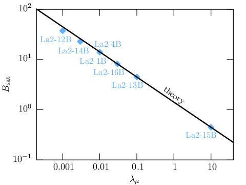
The parameter in the evolution Equation (4), or the corresponding dimensionless parameter in Equation (14), for the chiral chemical potential determines the nonlinear saturation of the chiral dynamo. We determine the saturation value of the magnetic field numerically for different values of ; see Figure 4. We find that the saturation value of the magnetic field increases with decreasing . This can be expected from the conservation law (8). If the initial magnetic energy is very small, we find from Equation (8) the following estimate for the saturated magnetic field during laminar chiral dynamo action:
| (29) |
where is the chiral chemical potential at saturation, and we use the estimate by . Inspection of Figure 4 demonstrates a good agreement between theoretical (solid line) and numerical results (blue diamonds).
III.2.6 Effect of a nonvanishing flipping rate
In this section, we consider the influence of a nonvanishing chiral flipping rate on the dynamo. A large flipping rate decreases the chiral chemical potential ; see Equation (4). It can stop the growth of the magnetic field caused by the chiral dynamo instability.
Quantitatively, the influence of the flipping term can be estimated by comparing the last two terms of Equation (4). The ratio of these terms is
| (30) |
where we have used Equation (29) with for the saturation value of the magnetic field strength. In Figure 5 we present the time evolution of and for different values of . The reference run La2-15B, with zero flipping rate (), has been repeated with a finite flipping term. As a result, the magnetic field grows more slowly in the nonlinear era, due to the flipping effect, and it decreases the saturation level of the magnetic field; see Figure 5. For larger values of , the chiral chemical potential decreases quickly, leading to strong quenching of the dynamo; see the blue lines in Figure 5.

III.3. Laminar chiral–shear dynamos
In this section, we consider laminar chiral dynamos in the presence of an imposed shearing velocity. Such a nonuniform velocity profile can be created in different astrophysical flows.
III.3.1 Theoretical aspects
We start by outlining the theoretical predictions for laminar chiral dynamos in the presence of an imposed shearing velocity; for details see Paper I. We consider the equilibrium configuration specified by the shear velocity , and const. This implies that the fluid has nonzero vorticity similar to differential (nonuniform) rotation. The functions and are determined by
| (31) | |||
| (32) |
We look for a solution to Equations (31) and (32) of the form . The growth rate of the dynamo instability and the frequency of the dynamo waves are given by
| (33) |
and
| (34) |
respectively. This solution describes a laminar –shear dynamo for arbitrary values of the shear rate .
Next, we consider a situation where the shear term on the right side of Equation (32) dominates, that is, where . The growth rate of the dynamo instability and the frequency of the dynamo waves are then given by
| (35) | |||
| (36) |
The dynamo is excited for . The maximum growth rate of the dynamo instability and the frequency of the dynamo waves are attained at
| (37) |
and are given by
| (38) | |||
| (39) |
This solution describes the laminar –shear dynamo.
III.3.2 Simulations of the laminar –shear dynamo
| simulation | |||||
|---|---|---|---|---|---|
| LaU-1B | 0.01 | 1.3 | 503 | ||
| LaU-1G | 0.01 | 1.3 | 503 | ||
| LaU-2B | 0.02 | 1.3 | 503 | ||
| LaU-2G | 0.02 | 1.3 | 503 | ||
| LaU-3B | 0.05 | 1.3 | 503 | ||
| LaU-3G | 0.05 | 1.3 | 503 | ||
| LaU-4B | 0.10 | 1.3 | 503 | ||
| LaU-4G | |||||
| LaU-5B | 0.20 | 1.3 | 503 | ||
| LaU-5G | 0.20 | 1.3 | 503 | ||
| LaU-6B | 0.50 | 1.3 | 503 | ||
| LaU-6G | 0.50 | 1.3 | 503 | ||
| LaU-7G | 0.01 | 4.0 | 283 | ||
| LaU-8G | 0.05 | 4.0 | 283 | ||
| LaU-9G | 0.10 | 4.0 | 283 | ||
| LaU-10G | 0.50 | 4.0 | 283 |

Since our simulations have periodic boundary conditions, we model shear velocities as . The mean shear velocity over half the box is . In Figure 6 we show the time evolution of the magnetic field (which starts to be excited from a Gaussian initial field), the velocity , the magnetic helicity , the chemical potential (multiplied by a factor of ), and for run LaU-4G. The growth rate for the chiral–shear dynamo (the –shear dynamo) is larger than that for the laminar chiral dynamo (the –dynamo). After a time of roughly , the system enters a nonlinear phase, in which the velocity field is affected by the magnetic field, but the magnetic field can still increase slowly. Saturation of the dynamo occurs after approximately .
For Gaussian initial fields, we have observed a short delay in the growth of the magnetic field. In both cases, the dynamo growth rate increases with increasing shear. As for the chiral dynamo, we observe perfect conservation of the quantity in the simulations of the laminar –shear dynamo.

In Figure 7 we show the theoretical dependence of the growth rate and the dynamo frequency on the shear velocity for Beltrami initial conditions at different wavenumbers; see Equations (35) and (38). The dynamo growth rate is estimated from an exponential fit. The result of the fit depends slightly on the fitting regime, leading to an error of the order of 10%. The dynamo frequency is determined afterward by dividing the magnetic field strength by and fitting a sine function. Due to the small amplitude and a limited number of periods of dynamo waves, the result is sensitive to the fit regime considered. Hence we assume a conservative error of 50% for the dynamo frequency. The blue diamonds correspond to the numerical results. Within the error bars, the theoretical and numerical results are in agreement.
III.3.3 Simulations of the laminar –shear dynamo

The growth rate of chiral–shear dynamos versus mean shear in the range between and is shown in Figure 8. We choose a large initial value of the chemical potential, i.e. , to ensure that is inside the box for all values of . We overplot the growth rates found from the simulations with the maximum growth rate given by Equation (33). In addition, we show the theoretical predictions for the limiting cases of the and –shear dynamos; see Equations (27) and (38). Inspection of Figure 8 shows that the results obtained from the simulations agree with theoretical predictions.
IV. Chiral magnetically driven turbulence
In this section we show that the CME can drive turbulence via the Lorentz force in the Navier-Stokes equation. When the magnetic field increases exponentially, due to the small-scale chiral magnetic dynamo with growth rate , the Lorentz force, , increases at the rate . The laminar dynamo occurs only up to the first nonlinear phase, when the Lorentz force starts to produce turbulence (referred to as chiral magnetically driven turbulence). We will also demonstrate here that, during the second nonlinear phase, a large-scale dynamo is excited by the chiral effect arising in chiral magnetically driven turbulence. The chiral effect was studied using different analytical approaches in Paper I. This effect is caused by an interaction of the CME and fluctuations of the small-scale current produced by tangling magnetic fluctuations. These fluctuations are generated by tangling of the large-scale magnetic field through sheared velocity fluctuations. Once the large-scale magnetic field becomes strong enough, the chiral chemical potential decreases, resulting in the saturation of the large-scale dynamo instability.
This situation is similar to that of driving small-scale turbulence via the Bell instability in a system with an external cosmic-ray current [10, 11], and the generation of a large-scale magnetic field by the Bell turbulence; see Rogachevskii et al. [88] for details.
IV.1. Mean-field theory for large-scale dynamos
In this section, we outline the theoretical predictions for large-scale dynamos based on mean-field theory; see Paper I for details. The mean induction equation is given by
where , and we consider the following equilibrium state: and . This mean-field equation contains additional terms that are related to the chiral effect and the turbulent magnetic diffusivity . In the mean-field equation, the chiral effect is replaced by the mean chiral effect. Note, however, that at large fluid and magnetic Reynolds numbers, the effect dominates the effect.
To study the large-scale dynamo, we seek a solution to Equation (), for small perturbations in the form , where is the unit vector directed along the axis. The functions and are determined by
| (41) |
| (42) |
where , and the other components of the magnetic field are and .
We look for a solution of the mean-field equations (41) and (42) in the form
| (43) |
where the growth rate of the large-scale dynamo instability is given by
| (44) |
with . The maximum growth rate of the large-scale dynamo instability, attained at the wavenumber
| (45) |
is given by
| (46) |
For small magnetic Reynolds numbers, , this equation yields the correct result for the laminar dynamo; see Equation (27).
As was shown in Paper I, the CME in the presence of turbulence gives rise to the chiral effect. The expression for found for large Reynolds numbers and a weak mean magnetic field is
| (47) |
Since the effect in homogeneous turbulence is always negative, while the effect is positive, the chiral effect decreases the effect. Both effects compensate each other at (see Paper I). However, for large fluid and magnetic Reynolds numbers, , and we can neglect in these equations. This regime corresponds to the large-scale dynamo.
IV.2. DNS of chiral magnetically driven turbulence
We have performed a higher resolution three-dimensional numerical simulation to study chiral magnetically driven turbulence. The chiral Mach number of this simulation is , the chiral nonlinearity parameter is , and the magnetic and the chiral Prandtl numbers are unity. The velocity field is initially zero, and the magnetic field is Gaussian noise, with .

The time evolution of , , , (multiplied by ), and of chiral magnetically driven turbulence is shown in the top panel of Figure 9. Four phases can be distinguished:
- (1)
The kinematic phase of small-scale chiral dynamo instability resulting in exponential growth of small-scale magnetic field due to the CME. This phase ends approximately at .
- (2)
The first nonlinear phase resulting in production of chiral magnetically driven turbulence. In this phase, grows from very weak noise over seven orders of magnitude up to nearly the equipartition value between turbulent kinetic and magnetic energies, due to the Lorentz force in the Navier-Stokes equation.
- (3)
The second nonlinear phase resulting in large-scale dynamos. In particular, the evolution of for is affected by the velocity field. During this phase, the velocity stays approximately constant, while the magnetic field continues to increase at a reduced growth rate in comparison with that of the small-scale chiral dynamo instability. In this phase, we also observe the formation of inverse energy transfer with a magnetic energy spectrum that was previously found and comprehensively analyzed by [24] in DNS of chiral MHD with different parameters.
- (4)
The third nonlinear phase resulting in saturation of the large-scale dynamos, which ends at when the large-scale magnetic field reaches the maximum value. The conserved quantity stays constant over all four phases. Saturation is caused by the term in the evolution equation of the chiral chemical potential, which leads to a decrease of from its initial value to 1.
The middle panel of Figure 9 shows the measured growth rate of as a function of time. In the kinematic phase, agrees with the theoretical prediction for the laminar chiral dynamo instability; see Equation (27), which is indicated by the dashed red horizontal line in the middle panel of Figure 9. During this phase, the growth rate of the velocity field, given by the dotted gray line in Figure 9, is larger by roughly a factor of two than that of the magnetic field. This is expected when turbulence is driven via the Lorentz force, which is quadratic in the magnetic field.
Once the kinetic energy is of the same order as the magnetic energy, the growth rate of the magnetic field decreases abruptly by a factor of more than five. This is expected in the presence of turbulence, because the energy dissipation of the magnetic field is increased by turbulence due to turbulent magnetic diffusion. Additionally, however, a positive contribution to the growth rate comes from the chiral effect that causes large-scale dynamo instability.
The time evolution of the ratio of the mean magnetic field to the total field, , is presented in the bottom panel of Figure 9. The mean magnetic field grows faster than the rms of the total magnetic field in the time interval between 0.14 and 0.2 . During this time, the large-scale (mean-field) dynamo operates, so magnetic energy is transferred to larger spatial scales. We now determine, directly from DNS, the growth rate of the large-scale dynamo using Equation (44). To this end, we determine the Reynolds number and the strength of the effect using the data from our DNS. Whereas the rms velocity is a direct output of the simulation, the turbulent forcing scale can be found from analysis of the energy spectra. The theoretical value based on these estimates at the time is indicated as the solid red horizontal line in the middle panel of Figure 9.

The evolution of kinetic and magnetic energy spectra is shown in Figure 10. We use equal time steps between the different spectra, covering the whole simulation time. The magnetic energy, indicated by blue lines, increases initially at , which agrees with the theoretical prediction for the chiral laminar dynamo. The magnetic field drives a turbulent spectrum of the kinetic energy, as can clearly be seen in Figure 10 (indicated by black lines in Figure 10). The final spectral slope of the kinetic energy is roughly . The magnetic field continues to grow at small wavenumbers, producing a peak at in the final stage of the time evolution.

We determine the correlation length of the magnetic field from the magnetic energy spectrum via
| (48) |
The wavenumber so defined coincides (up to a numerical factor of order unity) with the so-called tracking solution, in Boyarsky et al. [14]. There it was demonstrated that, in the course of evolution, the chiral chemical potential follows . And, indeed, the evolution of , shown in Figure 11, starts at around 10 (the value of in this simulation) and then decreases to (corresponding to the simulation box size) at . Interestingly, the chemical potential is affected by magnetic helicity only at much later times, as can be seen in Figure 11. Based on the wavenumber, , we estimate the Reynolds numbers as
| (49) |
Figure 11 shows that the Reynolds number increases exponentially, mostly due to the fast increase of , and saturates later at . Similarly, the turbulent diffusivity can be estimated as
| (50) |
During the operation of the mean-field large-scale dynamo, we find that , which is about 24 times larger than the molecular diffusivity . Using these estimates, we determine the chiral magnetic effect from Equation (47). The large-scale dynamo growth rate (44) is shown as the solid red horizontal line in the middle panel of Figure 9 and is in agreement with the DNS results shown as the black solid line.


Further analysis of the evolution of the magnetic field at different wavenumbers is presented in Figure 12. In the top panel, we display the magnetic energy at various wavenumbers as a function of time. In the kinematic phase, for , the fastest amplification occurs at , as can also be seen in the energy spectra. At wavenumbers there is an initial phase of magnetic dissipation, followed by an exponential increase of the field. The rapid transition between the two phases, which occurs at for in our example, may lead to the impression of an interpolation between long time steps. In reality, however, the range – is resolved by approximately 500 time steps. At , the magnetic field grows only at . This confirms the idea that a large-scale (mean-field) dynamo operates. In the next two panels, we compare the observed growth rates as a function of wavenumber at different time intervals. The middle panel of Figure 12 shows the growth rate in the laminar phase, where we find good agreement with the theoretical predictions below . The resulting value for the growth rate depends on the accuracy of the fitting, and a typical error of 10% is shown by a gray uncertainty band in the middle panel of Figure 12. Also, the observed growth rate of the mean-field dynamo, which we find from fitting growth rates in the time interval –, is comparable to the prediction from mean-field theory, using our estimates for the Reynolds number (49) and the turbulent diffusivity (50). As the mean-field dynamo phase is followed by the nonlinear phase, the growth rate is more sensitive to the fitting regime. Hence we indicate a 30% uncertainty band in this phase. The time intervals for the two different fitting regimes are indicated by gray arrows in the top panel.
IV.3. The effect of a strong initial magnetic field
The effect of changing the chiral nonlinearity parameter is explored in [24], who considered values between and . Using dimensional analysis and simulations, they showed that the extension of the inertial range of the turbulence is approximately . The ratio is approximately in our reference run for chiral magnetically driven turbulence, which was presented in the last section.
[24] found that is bound from above by the value of . It is interesting to note that this also applies when the initial magnetic field strength exceeds this limit. To demonstrate this, we now present a simulation with an initial magnetic energy spectrum for and exponential decrease for larger with . We use , , , and . The result is shown in Figure 13.

At early times, overshoots the value of , but after a short time it follows this limit almost precisely. This shows that the bound on is obeyed even when the initial field strength exceeds this value.
IV.4. Stages of chiral magnetically driven turbulence
This DNS demonstrates that the magnetic field evolution proceeds in the following distinct stages:
- (1)
Small-scale chiral dynamo instability.
- (2)
First nonlinear stage when the Lorentz force drives small-scale turbulence.
- (3)
Formation of inverse energy transfer with a magnetic energy spectrum; see [24] for details.
- (4)
Generation of large-scale magnetic fields by chiral magnetically driven turbulence.
- (5)
Decrease of the chemical potential and saturation of the large-scale chiral dynamo.
Although the magnetic field cannot grow any further, the spectrum continues to move to smaller wavenumbers in a shape-invariant fashion [19, see]. This implies that the magnetic integral scale continues to grow and the magnetic energy continues to decrease proportional to with .
V. DNS of large-scale dynamos in forced, nonhelical, and homogeneous turbulence
In this section, we study the evolution of the magnetic field in the presence of forced, nonhelical, and homogeneous turbulence in order to control the turbulence parameters in the chiral MHD simulations. Chiral dynamos in forced turbulence can be described by the mean-field chiral MHD equations. The theoretical results related to the mean-field chiral dynamos obtained in Paper I have been outlined in Section IV.1.
V.1. DNS setup for externally forced turbulence
To study chiral large-scale dynamos, we perform three-dimensional DNS with externally forced turbulence and a spatial resolution of . In run Ta2-10, the resolution is (see Table 3). Turbulence is driven via the forcing term in Equation (2). The forcing function is nonhelical and localized around the wavenumber ; see [58] for details. For the runs presented in the following, we choose and 10. These values are small enough for the fluid and magnetic Reynolds numbers, and , respectively, to be sufficiently large for turbulence to develop. At the same time, is large enough for a clear separation between the box scale and the forcing scale, allowing to study of mean-field (large-scale) dynamos. In the numerical simulations, we vary , , and (see Table 3).
For comparison with the results from mean-field theory, the simulations need to
fulfill the following criteria:
- •
To capture the maximum amplification inside the numerical domain with , the condition needs to be fulfilled. As shown in Equation (45), is proportional to , which is inversely proportional to the magnetic Reynolds number . As a result, the chemical potential needs to be sufficiently large for .
- •
Due to nonlocal effects, the turbulent diffusivity is generally scale-dependent and decreases above [22]. For comparison with mean-field theory, the chiral dynamo instability has to occur on scales , where . Note, however, that the presence of a mean kinetic helicity in the system caused by the CME (see Paper I) can increase the turbulent diffusivity for moderate magnetic Reynolds numbers by up to 50% [23].
- •
To simplify the system, we avoid classical small-scale dynamo action, which occurs at magnetic Reynolds numbers larger than .
| (early late) | |||||||
|---|---|---|---|---|---|---|---|
| Ta2-1 | 160 | 4.5 | |||||
| Ta2-2 | 80 | 63 | |||||
| Ta2-3 | 160 | 45 | |||||
| Ta2-4 | 80 | 63 | |||||
| Ta2-5 | |||||||
| Ta2-6 | 51 | 80 | |||||
| Ta2-7 | 230 | 38 | |||||
| Ta2-8 | 160 | 43 | |||||
| Ta2-9 | 150 | 47 | |||||
| Ta2-10 | 160 | 45 |
V.2. DNS of chiral dynamos in forced turbulence

The time evolution of different quantities in our reference run is presented in Figure 14. The magnetic field first increases first exponentially, with a growth rate , which is about a factor of 1.6 lower than that expected for the laminar dynamo; see the middle panel of Figure 14. This difference seems to be caused by the presence of random forcing; see discussion below. At approximately 0.2 , the growth rate decreases to a value of consistent with that of the mean-field chiral dynamo, before saturation occurs at . The evolution of is comparable qualitatively in chiral magnetically produced turbulence; see Figure 9. An additional difference from the latter is the value of for externally forced turbulence, which is controlled by the intensity of the forcing function. An indication of the presence of a mean-field dynamo is the evolution of in the bottom panel of Figure 14, which reaches a value of unity at .
The energy spectra presented in Figure 15 support the large-scale dynamo scenario. First, the magnetic energy increases at all scales, and, at later times, the maximum of the magnetic energy is shifted to smaller wavenumbers, finally producing a peak at , i.e., the smallest possible wavenumber in our periodic domain.
A detailed analysis of the growth of magnetic energy is presented in Figure 16. In the first phase, the growth rate of the magnetic field is independent of the wavenumber (see top panel), due to a coupling between different modes. The growth rate measured in this phase is less than that in the laminar case (see middle panel), due to a scale-dependent turbulent diffusion caused by the random forcing.
Within the time interval –, only the magnetic field at increases. This is clearly seen in the bottom panel of Figure 16, where we show the evolution of the magnetic energy at different wavenumbers . The growth rate of the mean-field dynamo, which is determined at , agrees with the result from mean-field theory, given by Equation (51). There is a small dependence of the resulting mean-field growth rate on the exact fitting regime. If the phase of the mean-field dynamo is very short, changing the fitting range can affect the result by a factor up to 30 %. We use the latter value as an estimate of the uncertainty in the growth rate, and, in addition, indicate an error of 20 % in determining the Reynolds number, which is caused by the temporal variations of .


V.3. Dependence on the magnetic Reynolds number
Based on the mean-field theory developed in Paper I, we expect the following. Using the expression for the effect given by Equation (47), the maximum growth rate (46) for the mean-field dynamo can be rewritten as a function of the magnetic Reynolds number:
| (51) |
where the ratio .
We perform DNS with different Reynolds numbers to test the scaling of given by Equation (51). The parameters of the runs with externally forced turbulence are summarized in Table 3. We vary ), the forcing wavenumber , as well as the amplitude of the forcing, to determine the function . In the initial phase, is constant in time. Once large-scale turbulent dynamo action occurs, there are additional minor variations in , because the system is already in the nonlinear phase. The nonlinear terms in the Navier-Stokes equation lead to a modification of the velocity field at small spatial scales, which affects the value of and results in the small difference between the initial and final values of the Reynolds numbers (see Table 3).
According to Equation (45), the wavenumber associated with the maximum growth rate of the large-scale turbulent dynamo instability decreases with increasing . In order to keep this mode inside the computational domain and hence to compare the measured growth rate with the maximum one given by Equation (51), we vary the value of in our simulations. The variation of and the additional variation of for scanning through the parameter space, implies that changes correspondingly.
The values of the nonlinear parameter should be within a certain range. Indeed, the saturation value of the magnetic field, given by Equation (29), is proportional to . In order for the Alfvén velocity not to exceed the sound speed, which would result in a very small time step in DNS, should not be below a certain value. On the other hand, should not be too large, as in this case the dynamo would saturate quickly, and there is only a very short time interval of the large-scale dynamo. In this case, determining the growth rate of the mean-field dynamo, and hence comparing with the mean-field theory, is difficult.

In Figure 17 we show the normalized growth rate of the magnetic field as a function of the magnetic Reynolds number . The gray data points show the growth rate in the initial, purely kinematic phase of the simulations. The blue data points show the measured growth rate of the magnetic field on , when the large-scale dynamo occurs. For comparison of the results with externally forced turbulence (indicated as diamond-shaped data points), we show in Figure 17 also the results obtained for the dynamo in chiral magnetically driven turbulence, which are indicated as dots.
In DNS with externally forced turbulence, we see in all cases a reduced growth rate due to mode coupling. Contrary to the case with externally forced turbulence, in DNS with the chiral magnetically driven turbulence, we do initially observe the purely laminar dynamo with the growth rate given by Equation (27), because there is no mode coupling in the initial phase of the magnetic field evolution in this case. On the other hand, the measured growth rates of the mean-field dynamo in both cases agree (within the error bars) with the growth rates obtained from the mean-field theory.
VI. Chiral MHD dynamos in astrophysical relativistic plasmas
In this section, the results for the nonlinear evolution of the chiral chemical potential, the magnetic field, and the turbulent state of the plasma found in this paper are applied to astrophysical relativistic plasmas. We begin by discussing the role of chiral dynamos in the early universe and identify conditions under which the CME affects the generation and evolution of cosmic magnetic fields. Finally, in Section VI.2, we examine the importance of the CME in proto-neutron stars (PNEs).
VI.1. Early Universe
In spite of many possible mechanisms that can produce magnetic fields in the early universe [see, e.g., 112, 113, 40, 53, 99, for reviews], understanding the origin of cosmic magnetic fields remains an open problem. Their generation is often associated with nonequilibrium events in the universe (e.g., inflation or phase transitions). A period of particular interest is the electroweak (EW) epoch, characterized by temperatures of (). Several important events take place around this time: the electroweak symmetry gets broken, photons appear while intermediate vector bosons become massive, and the asymmetry between matter and antimatter appears in the electroweak baryogenesis scenario [68]; see, for example, the review by Morrissey & Ramsey-Musolf [73]. Magnetic fields of appreciable strength can be generated as a consequence of these events [106, 76, 47, 46, 108, 52, 33, 7, 107, 93]. Their typical correlation length corresponds to only a few centimeters today – much less than the observed correlation scales of magnetic fields in galaxies or galaxy clusters. Therefore, in the absence of mechanisms that can increase the comoving scale of the magnetic field beyond , such fields were deemed to be irrelevant to the problem of cosmic magnetic fields [39, 27, 90, 63, for discussion, see, e.g.,].
The situation may change if (i) the magnetic fields are helical and (ii) the plasma is turbulent. In this case, an inverse transfer of magnetic energy may develop, which leads to a shift of the typical scale of the magnetic field to progressively larger scales [18, 31, 6, 63]. The origin of such turbulence has been unknown. An often considered paradigm is that a random magnetic field, generated at small scales, produces turbulent motions via the Lorentz force. However, continuous energy input is required. If this is not the case, the magnetic field decays: as the correlation scale grows [13, 63], so that .
In the present work, we demonstrated that the presence of a finite chiral charge in the plasma at the EW epoch is sufficient to satisfy the above requirements (i) and (ii). As a result,
- (1)
helical magnetic fields are excited,
- (2)
turbulence with large is produced, and
- (3)
the comoving correlation scale increases.
We discuss each of these phases in detail below.
VI.1.1 Generation and evolution of cosmic magnetic fields in the presence of a chiral chemical potential
Although it is not possible to perform numerical simulations with parameters matching those of the early universe, the results of the present paper allow us to make qualitative predictions about the fate of cosmological magnetic fields generated at the EW epoch in the presence of a chiral chemical potential.
All of the main stages of the magnetic field evolution, summarized in Section IV.4, can occur in the early universe (a sketch of the main phases is provided in Figure 18).

Phase 1. At this initial stage, the small-scale chiral dynamo instability develops at scales around , where
| (52) |
and
| (53) |
The chemical potential can be approximated by the thermal energy for order-of-magnitude estimates. In what follows, we provide numerical estimates for which corresponds to the typical thermal energy of relativistic particles at the EW epoch. The characteristic energy at the quantum chromodynamics phase transition is where the quark–gluon plasma turns into hadrons. We stress, however, that the MHD formalism is only valid if the scales considered are larger than the mean free path given by Equation (6). Comparing the chiral instability scale with results in the condition . Strictly speaking, modeling a system that does not fulfill this condition requires full kinetic theory as described, for example, in Chen et al. [30] or in Akamatsu & Yamamoto [1].
The growth rate of an initially weak magnetic field in the linear stage of the chiral dynamo instability is given by Equation (27):
| (54) |
For the value of the magnetic diffusivity in the early universe, we adopted the conductivity from Equation (1.11) of [4]. Numerically,
| (55) |
where (so that ). As a result, the number of -foldings over one Hubble time is
where
| (56) |
(here is the number of relativistic degrees of freedom and ). We should stress that this picture has been known before and was described in many previous works [61, 49, 50, 14].
We note that a nonzero chiral flipping rate has been discussed in the literature [26, 14, 44, 15, 94]. In Section III.2.6, we have found in numerical simulations that the flipping term affects the evolution of the magnetic field only for large values of , when the flipping term is of the order of or larger than the term in Equation (14); see also Equation (30) and Figure 5. When adopting the estimate in Brandenburg et al. [24] of , chirality flipping is not likely to play a significant role for the laminar dynamo in the early universe at very high temperatures of the order of . However, depends on the ratio and thus suppresses all chiral effects once the universe has cooled down to [14]. At this point, we stress again that the true value of is unknown and has here been set to the thermal energy in Equation (53). If it turns out that the initial value of the chiral chemical potential is much smaller than the thermal energy, becomes larger, and the flipping rate can play a more important role already during the initial phases of the chiral instability in the early universe. This scenario is not considered in the following discussion.
In the regime of the laminar dynamo, one could reach -folds over the Hubble time ; see lower panel of Figure 19. However, as shown in this work, already after a few hundred -foldings, the magnetic field starts to excite turbulence via the Lorentz force. This happens once the magnetic field is no longer force-free. Once the flow velocities reach the level , nonlinear terms are no longer small, small-scale turbulence is produced, and the next phase begins.
Phase 2. The subsequent evolution of the magnetic field depends on the strength of the chiral magnetically excited turbulence. This has been shown in the mean-field analysis of Rogachevskii et al. [89] and is confirmed by the present work; see, for example, Figure 17. The growth rate and instability scale depend on the magnetic Reynolds number; see Equations (44)–(46). The maximum growth rate for is given by
| (57) |
where is given by Equation (54). For the early universe, it is impossible to determine the exact value of the magnetic Reynolds number from the numerical simulations, but one expects and we show in Figure 19 that, in a wide range of magnetic Reynolds numbers, , the number of -foldings during one Hubble time is much larger than . The turbulence efficiently excites magnetic fields at scales much larger than (Figure 19, top panel).

Using dimensional analysis and DNS, Brandenburg et al. [24] demonstrated that the resulting spectrum of the magnetic fields behaves as between and , given by Equation (21). The wavenumber depends on the nonlinearity parameter , defined by Equation (5), which, in the early universe, is given by
| (58) |
We note that this expression is, strictly speaking, only valid when and modifications might be expected outside of this regime. Further, the mean density of the plasma
| (59) |
The ratio is presented in the top panel of Figure 19, but we note that the exact numerical coefficient in the condition might depend on .
Phase 3. The stage of large-scale turbulent dynamo action ends with the saturation phase (see Section IV.4 and Figure 18). At this stage, the total chiral charge (determined by the initial conditions) gets transferred to magnetic helicity. As shown in Boyarsky et al. [14] (see also Joyce & Shaposhnikov [61] for earlier work, as well as [100] and [60] for more discussion), and confirmed by numerical simulations in Brandenburg et al. [24] and in the present work, the chiral chemical potential follows at this stage and thus decreases with time. Therefore, most of the chiral charge will be transferred with time into magnetic helicity,
| (60) |
switching off the CME (the end of Phase 3 in Figure 18).
VI.1.2 Chiral MHD and cosmic magnetic fields
Magnetic fields produced by chiral dynamos are fully helical. Once the CME has become negligible, the subsequent phase of decaying helical turbulence begins and the magnetic energy decreases, while the magnetic correlation length increases in such a way that the magnetic helicity (60) is conserved for very small magnetic diffusivity [13, 63].
Based on Equation (60), one can estimate the magnetic helicity today; see also [24]. Taking as an estimate for the chiral chemical potential (this means that the density of the chiral charge is of the order of the number density of photons), one finds
| (61) |
Here, the present number density of photons is , and the ratio of the effective relativistic degrees of freedom today and at the EW epoch appears, because the photon number density dilutes as while the magnetic helicity dilutes as . We recall that, to arrive at the numerical value in given in Equation (61), an additional factor was applied to convert to Gaussian units.
Under the assumption that the spectrum of the cosmic magnetic field is sharply peaked at some scale (as is the case in all of the simulations presented here), the lower bounds on magnetic fields, inferred from the nonobservation of GeV cascades from TeV sources [74, 101, 36] can be directly translated into a bound on magnetic helicity today. The observational bound scales as for [74] and therefore . The numerical value is obtained using the most conservative bound at (Dermer et al. 34, see also Durrer & Neronov 40). These observational constraints for intergalactic magnetic fields are compared to the magnetic field produced in chiral MHD for different values of the initial chiral chemical potential in Figure 20.
The limit given by Equation (61) is quite general. It does not rely on chiral MHD or the CME, but simply reinterprets the bounds of [74], [101], [36], and [34] as bounds on magnetic helicity. Given such an interpretation, we conclude that if cosmic magnetic fields are helical and have a cosmological origin, then at some moment in the history of the universe the density of chiral charge was much larger than . This chiral charge can be, for example, in the form of magnetic helicity or of chiral asymmetry of fermions, or both. To generate such a charge density, some new physics beyond the Standard Model of elementary particles is required. Below we list several possible mechanisms that can generate large initial chiral charge density:

- (1)
The upper bound in Equation (61) assumes that only one fermion of the Standard Model developed a chiral asymmetry . Many fermionic species are present in the plasma at the electroweak epoch. They all can have a left–right asymmetric population of comparable size, increasing the total chirality by a factor , which makes the estimate (61) consistent with the lower bound from Dermer et al. [34]. One should check, of course, whether for more massive fermions the chirality flipping rate is much slower than the dynamo growth rate determined by Equation (54).
- (2)
- (3)
The left–right asymmetry may be produced as a consequence of the decay of helical hypermagnetic fields prior to the EW epoch. Such a scenario, relating hypermagnetic helicity to the chiral asymmetry, has been discussed previously, such as in [54] and [92]. A conservation law similar to that of (10) exists also for hypermagnetic fields, and the decay of the latter may cause asymmetric populations of left and right states.
- (4)
From the point of view of chiral MHD, the value of (to which this bound is proportional) is just an initial condition and therefore can take arbitrary values. Once an initial condition with a large value of has been generated, the subsequent evolution (as described above) does not require any new physics.
Moreover, the coupled evolution of magnetic helicity and chiral chemical potential is unavoidable in the relativistic plasma and should be an integral part of relativistic MHD (as was discussed in Paper I).
VI.2. PNSs and the CME
In this section, we explore whether the CME and chiral dynamos can play a role in the development of strong magnetic fields in neutron stars. A PNS is a stage of stellar evolution after the supernova core collapse and before the cold and dense neutron star is formed [81, see, e.g.,]. PNSs are characterized by high temperatures (typically ), large lepton number density (electrons Fermi energy a few hundreds of MeV), the presence of turbulent flows in the interior, and quickly changing environments. Once the formation of a neutron star is completed, its magnetic field can be extremely large. Neutron stars that exceed the quantum electrodynamic limit are known as “magnetars” [see, e.g., 71, 105, 64, for recent reviews]. The origin of such strong magnetic fields remains unknown, although many explanations have been proposed; see, for example, Duncan & Thompson [38], [2], and [48].
The role of the CME in the physics of (proto)neutron stars and their contribution to the generation of strong magnetic fields have been discussed in a number of works [28, 75, 43, 44, 55, 41, 94, 114].
VI.2.1 Chiral MHD in PNSs
During the formation of a PNS, electrons and protons are converted into neutrons, leaving behind left-handed neutrinos. This is known as the Urca process [57, ;]. If the chirality-flipping timescale, determined by the electron’s mass, is longer than the instability scale, the net chiral asymmetry in the PNS can lead to the generation of magnetic fields. This scenario has been discussed previously [75, 94, 55]. The chiral turbulent dynamos discussed in this work can be relevant for the physics of PNSs and can affect our conclusions about the importance of the CME. However, to make a detailed quantitative analysis, a number of factors should be taken into account:
- (1)
- (2)
- (3)
The neutrinos produced via the Urca process are trapped in the interior of a PNS and can release the chiral asymmetry back into the plasma via the process. Therefore, only when the star becomes transparent to neutrinos (as the temperature drops to a few MeV) does the creation of chiral asymmetry can become significant.
Modeling the details of PNS cooling and neutrino propagation is beyond the scope of this paper. Below we perform the estimates that demonstrate that chiral MHD can significantly change the picture of the evolution of a PNS.
VI.2.2 Estimates of the relevant parameters
An upper limit of the chiral chemical potential can be estimated by assuming that and (all left-chiral electrons have been converted into neutrinos, and the rate of chirality flipping is much slower than other relevant processes). This leads to the estimate and correspondingly
| (62) |
where we have used a typical value of the electron’s Fermi energy [81]. For an ultrarelativistic degenerate electron gas (i.e., when ), the relation between the number density of electrons, , and their Fermi energy, , is
| (63) |
The interior of neutron stars is a conducting medium whose conductivity is estimated to be [8, 65]:
| (64) | |||||
| (65) |
(there is actually a difference in the numerical coefficient between the results of Baym et al. [8] and Kelly [65]). Using Equation (65), we find the magnetic diffusion coefficient to be
| (66) |
Therefore, we can determine the the maximum growth rate of the small-scale chiral instability (27) as
| (67) |
We see that over a characteristic time (the typical cooling time), the magnetic field would increase by many -foldings. In fact, using a flipping rate of , as suggested in Grabowska et al. [55] for and , we find that ranges from down to for the range between and . Hence the evolution of the chemical potential and the chiral dynamo is weakly affected by flipping reactions.
As in Section VI.1.1, the phase of the small-scale instability ends when turbulence is excited. It should be stressed, however, that unlike the early universe, the interiors of PNSs are expected to be turbulent with high even in the absence of chiral effects (with as large as ); see [102]. Therefore, the system may find itself in the forced turbulence regime of Section V.2. Figure 21 shows that in a wide range of magnetic Reynolds numbers, one can have many -foldings over a typical timescale of the PNS and that the scale of the magnetic field can reach macroscopic size.

VI.2.3 Estimate of magnetic field strengths
A dedicated analysis, taking into account temperature and density evolution of the PNS as well as its turbulent regimes, is needed to make detailed predictions. Here we will make the estimates of the strength of the magnetic field, similar to Section VI.1 above. To this end, we use the conservation law (10), assuming . In the PNS case, the plasma is degenerate, and therefore the relation between and is given by
| (68) |
(in the limit ). As a result, the chiral feedback parameter is
| (69) |
which determines the wavenumber ; see Equation (21). The corresponding length scale is presented in the top panel of Figure 21, where we assume a mean density of the PNS of .
Using Equations (62) and (69), we find
| (70) | |||||
| (71) |
Assuming for the maximum correlation scale (see Figure 21), we find that magnetic field strength is of the order of
| (72) |
Notice that the estimate (70) is independent of (but depends strongly on the assumed value of ).
Our estimates have demonstrated that the chiral MHD could be capable of generating strong small-scale magnetic fields. Therefore, chiral effects should be included in the modeling of evolution of PNSs.
VII. Conclusions
In this work, we have presented results from numerical simulations of chiral MHD that include the temporal and spatial evolution of magnetic fields, plasma motions, and the chiral chemical potential. The latter, characterizing the asymmetry between left- and right-handed fermions, gives rise to the CME, which results in the excitation of a small-scale chiral dynamo instability.
Our numerical simulations are performed for the system of chiral MHD equations (1)–(4) that was derived in Paper I. This system of equations is valid for plasmas with high electric conductivity, that is, in the limit of high and moderately high Reynolds numbers. Chiral flipping reactions are neglected in most of the simulations. In the majority of the runs, the initial conditions are a very weak magnetic seed field and a high chiral chemical potential. Both initially force-free systems and systems with external forcing of turbulence are considered. With our numerical simulations, we confirm various theoretical predictions of the chiral laminar and turbulent large-scale dynamos discussed in Paper I.
Our findings from DNS can be summarized as follows:
- •
The evolution of magnetic fields studied here in DNS agrees with the predictions made in Paper I for all types of laminar dynamos. In particular, the scalings of the maximum growth rate of the chiral dynamo instability for the dynamo (see Figure 2) and for the –shear dynamo (see Figure 7) have been confirmed. Additionally, the transitional regime of an –shear dynamo, where the contributions from the - and shear terms are comparable, agrees with theoretical predictions, as can be seen in Figure 8. In our DNS, the scale-dependent amplification of the magnetic field in the laminar chiral dynamo is observed in the energy spectra; see, for example, Figure 10 where the maximum growth rate of the dynamo instability is attained at wavenumber .
- •
- •
The CME can drive turbulence efficiently via the Lorentz force, which has been demonstrated in our numerical simulations through the measured growth rate of the turbulent velocity, which is larger by approximately a factor of two than that of the magnetic field; see, for example, the middle panel of Figure 9.
- •
In the presence of small-scale turbulence, the large-scale dynamo operates due to the chiral effect, which is not related to the kinetic helicity; see Equation (47). In the limit of large magnetic Reynolds numbers, the maximum growth rate of the large-scale dynamo instability is reduced by a factor of as compared to the laminar case; see Equation (51). The dynamo growth rate is close to this prediction of mean-field chiral MHD for both chiral magnetically produced turbulence and for externally driven turbulence; see see Figure 17.
- •
Using DNS, we found a new scenario of the magnetic field evolution consisting of three phases (see also the schematic overview in Figure 18):
- (1)
small-scale chiral dynamo instability;
- (2)
production of small-scale turbulence, inverse transfer of magnetic energy, and generation of a large-scale magnetic field by the chiral effect;
- (3)
saturation of the large-scale chiral dynamo by a decrease of the CME controlled by the conservation law for the total chirality: .
The previously discussed scenario of magnetic field evolution caused by the CME [14] did not include the second phase.
- (1)
While the results summarized above have been obtained in simulations of well-resolved periodic domains, astrophysical parameters are beyond the regime accessible to DNS. Hence we can only estimate the effects of the chiral anomaly in relativistic astrophysical plasmas, like in the early universe or in neutron stars. The main conclusions from the astrophysical applications are the following:
- •
The chiral MHD scenario found in DNS may help to explain the origin of the magnetic field observed in the interstellar medium. The chiral dynamo instability produces helical magnetic fields initially at small spatial scales and simultaneously drives turbulence, which generates a magnetic field on large scales. After the chiral chemical potential has been transformed into magnetic helicity during the dynamo saturation phase, the magnetic field cascades to larger spatial scales according to the phenomenology of decaying MHD turbulence. We have estimated the values of and for the early universe. These parameters determine the time and spatial scales associated with the chiral dynamo instability (see Figure 19) and the maximum magnetic helicity (see Equation 61). Our estimates for magnetic fields produced by chiral dynamos in the early universe are consistent with the observational lower limits found by Dermer et al. [34] (see Figure 20) if we assume that the initial chiral chemical potential is of the order of the thermal energy density.
- •
In PNSs, chiral dynamos operating in the first tens of seconds after the supernova explosion can produce magnetic fields of approximately at a magnetic correlation length of ; see Equation (72). However, we stress that many questions remain open, especially regarding the generation of a chiral asymmetry and the role of the chiral flipping term in PNEs.
Finally, we stress again that the parameters and the initial conditions, including the initial chiral asymmetry, are unknown in the astrophysical systems discussed in this paper. Hence, the purpose of our applications should be classified as a study of the conditions under which the CME plays a significant role in the evolution of a plasma of relativistic charged fermions. With the regimes accessible to our simulations not being truly realistic in the context of the physics of the early universe and in neutron stars, our applications have a rather exploratory nature. In this sense, our results from DNS can be used to answer the question in which area of plasma physics – the physics of the early universe, the physics of neutron stars, or the physics of heavy ion collisions—the CME is important and can modify the evolution of magnetic fields.
References
- [1] Akamatsu, Y., & Yamamoto, N. 2013, Physical Review Letters, 111, 052002
- [2] Akiyama, S., Wheeler, J. C., Meier, D. L., & Lichtenstadt, I. 2003, ApJ, 584, 954
- [3] Alekseev, A. Y., Cheianov, V. V., & Fröhlich, J. 1998, Phys. Rev. Lett., 81, 3503
- [4] Arnold, P., Moore, G. D., & Yaffe, L. G. 2000, J. High Energy Phys., 11, 001
- [5] Artsimovich, L. A., & Sagdeev, R. Z. 1985, Plasma Physics for Physicists (Benjamin, New York)
- [6] Banerjee, R., & Jedamzik, K. 2004, Phys. Rev. D, 70, 123003
- [7] Baym, G., Bödeker, D., & McLerran, L. 1996, Phys. Rev. D, 53, 662
- [8] Baym, G., Pethick, C., & Pikes, D. 1969, Nature, 224, 674
- [9] Beck, R. 2015, A&A Rev., 24, 4
- [10] Bell, A. R. 2004, MNRAS, 353, 550
- [11] Beresnyak, A., & Li, H. 2014, ApJ, 788, 107
- [12] Biskamp, D. 1997, Nonlinear Magnetohydrodynamics (Cambridge University Press)
- [13] Biskamp, D., & Müller, W.-C. 1999, Phys. Rev. Lett., 83, 2195
- [14] Boyarsky, A., Fröhlich, J., & Ruchayskiy, O. 2012, Phys. Rev. Lett., 108, 031301
- [15] ——. 2015, Phys. Rev. D, 92, 043004
- [16] Brandenburg, A. 2003, in Advances in Nonlinear Dynamics, ed. A. Ferriz-Mas & M. Núñez (Taylor & Francis, London and New York), 269
- [17] Brandenburg, A., & Dobler, W. 2002, Comp. Phys. Comm., 147, 471
- [18] Brandenburg, A., Enqvist, K., & Olesen, P. 1996, Phys. Rev. D, 54
- [19] Brandenburg, A., & Kahniashvili, T. 2017, Phys. Rev. Lett., 118, 055102
- [20] Brandenburg, A., Kahniashvili, T., & Tevzadze, A. G. 2015, Phys. Rev. Lett., 114, 075001
- [21] Brandenburg, A., Nordlund, A., Stein, R. F., & Torkelsson, U. 1995, ApJ, 446, 741
- [22] Brandenburg, A., Rädler, K.-H., & Schrinner, M. 2008, A&A, 482, 739
- [23] Brandenburg, A., Schober, J., & Rogachevskii, I. 2017a, Astron. Nachr., 338, 790
- [24] Brandenburg, A., Schober, J., Rogachevskii, I., Kahniashvili, T., Boyarsky, A., Fröhlich, J., Ruchayskiy, O., & Kleeorin, N. 2017b, ApJL, 845, L21
- [25] Brandenburg, A., & Subramanian, K. 2005, Phys. Rept., 417, 1
- [26] Campbell, B. A., Davidson, S., Ellis, J., & Olive, K. A. 1992, Phys. Lett. B, 297, 118
- [27] Caprini, C., Durrer, R., & Fenu, E. 2009, JCAP, 0911, 001
- [28] Charbonneau, J., & Zhitnitsky, A. 2010, JCAP, 1008, 010
- [29] Charbonneau, P. 2014, ARA&A, 52, 251
- [30] Chen, J.-W., Pu, S., Wang, Q., & Wang, X.-N. 2013, Physical Review Letters, 110, 262301
- [31] Christensson, M., Hindmarsh, M., & Brandenburg, A. 2001, Phys. Rev. E, 64, 056405
- [32] Crutcher, R. M. 2012, ARA&A, 50, 29
- [33] Davidson, S. 1996, Phys. Lett. B, 380, 253
- [34] Dermer, C. D., Cavadini, M., Razzaque, S., Finke, J. D., Chiang, J., & Lott, B. 2011, ApJ, 733, L21
- [35] Devlen, E., Brandenburg, A., & Mitra, D. 2013, MNRAS, 432, 1651
- [36] Dolag, K., Kachelriess, M., Ostapchenko, S., & Tomas, R. 2011, ApJ, 727, L4
- [37] Donati, J.-F., & Landstreet, J. D. 2009, ARA&A, 47, 333
- [38] Duncan, R. C., & Thompson, C. 1992, ApJ, 392, L9
- [39] Durrer, R., & Caprini, C. 2003, JCAP, 0311, 010
- [40] Durrer, R., & Neronov, A. 2013, A&A Rev., 21, 62
- [41] Dvornikov, M. 2016
- [42] Dvornikov, M., & Semikoz, V. B. 2015a, Phys. Rev. D, 92, 083007
- [43] ——. 2015b, JCAP, 1505, 032
- [44] ——. 2015c, Phys. Rev. D, 91, 061301
- [45] ——. 2017, Phys. Rev. D, 95, 043538
- [46] Enqvist, K. 1994, in 1st International Conference on Strong and Electroweak Matter (SEWM 1994) Sintra, Portugal, March 23-25, 1994, 143–154
- [47] Enqvist, K., & Olesen, P. 1993, Phys. Lett. B, 319, 178
- [48] Ferrario, L., & Wickramasinghe, D. 2006, MNRAS, 367, 1323
- [49] Fröhlich, J., & Pedrini, B. 2000, in Mathematical Physics 2000, ed. A. S. Fokas, A. Grigoryan, T. Kibble, & B. Zegarlinski, International Conference on Mathematical Physics 2000, Imperial college (London) (World Scientific Publishing Company)
- [50] Fröhlich, J., & Pedrini, B. 2002, in Statistical Field Theory, ed. A. Cappelli & G. Mussardo (Kluwer)
- [51] Fukushima, K., Kharzeev, D. E., & Warringa, H. J. 2008, Phys. Rev. D, 78, 074033
- [52] Gasperini, M., Giovannini, M., & Veneziano, G. 1995, Phys. Rev. Lett., 75, 3796
- [53] Giovannini, M. 2004, Int. J. Mod. Phys. D, 13, 391
- [54] Giovannini, M., & Shaposhnikov, M. E. 1998, Phys. Rev. D, 57, 2186
- [55] Grabowska, D., Kaplan, D. B., & Reddy, S. 2015, Phys. Rev. D, 91, 085035
- [56] Grasso, D., & Rubinstein, H. R. 2001, Phys. Rep., 348, 163
- [57] Haensel, P. 1995, Space Sci. Rev., 74, 427
- [58] Haugen, N. E., Brandenburg, A., & Dobler, W. 2004, Phys. Rev. E, 70, 016308
- [59] Hawley, J. F., Gammie, C. F., & Balbus, S. A. 1995, ApJ, 440, 742
- [60] Hirono, Y., Kharzeev, D., & Yin, Y. 2015, Phys. Rev. D, 92, 125031
- [61] Joyce, M., & Shaposhnikov, M. 1997, Phys. Rev. Lett., 79, 1193
- [62] Kahniashvili, T., Maravin, Y., Natarajan, A., Battaglia, N., & Tevzadze, A. G. 2013a, ApJ, 770, 47
- [63] Kahniashvili, T., Tevzadze, A. G., Brandenburg, A., & Neronov, A. 2013b, Phys. Rev. D, 87, 083007
- [64] Kaspi, V. M., & Beloborodov, A. M. 2017, ARA&A, 55, 261
- [65] Kelly, D. C. 1973, ApJ, 179, 599
- [66] Krause, F., & Rädler, K. H. 1980, Mean-Field Magnetohydrodynamics and Dynamo Theory (Pergamon, Oxford)
- [67] Kulsrud, R. M., & Zweibel, E. G. 2008, Rep. Prog. Phys., 71, 046901
- [68] Kuzmin, V. A., Rubakov, V. A., & Shaposhnikov, M. E. 1985, Physics Letters B, 155, 36
- [69] Lattimer, J. M., Prakash, M., Pethick, C. J., & Haensel, P. 1991, Phys. Rev. Lett., 66, 2701
- [70] Melrose, D. 2012, Quantum Plasma Dynamics: Magnetized Plasmas (Springer, New York)
- [71] Mereghetti, S., Pons, J. A., & Melatos, A. 2015, Space Sci. Rev., 191, 315
- [72] Moffatt, H. K. 1978, Magnetic Field Generation in Electrically Conducting Fluids (Cambridge, England, Cambridge University Press)
- [73] Morrissey, D. E., & Ramsey-Musolf, M. J. 2012, New Journal of Physics, 14, 125003
- [74] Neronov, A., & Vovk, I. 2010, Science, 328, 73
- [75] Ohnishi, A., & Yamamoto, N. 2014
- [76] Olesen, P. 1992, Phys. Lett. B, 281, 300
- [77] Pandey, K. L., Choudhury, T. R., Sethi, S. K., & Ferrara, A. 2015, MNRAS, 451, 1692
- [78] Parker, E. 1979, Cosmical Magnetic Fields (Oxford University Press, New York)
- [79] Parker, E. N. 1955, ApJ, 122, 293
- [80] Pavlović, P., Leite, N., & Sigl, G. 2017, Phys. Rev. D, 96, 023504
- [81] Pons, J. A., Reddy, S., Prakash, M., Lattimer, J. M., & Miralles, J. A. 1999, ApJ, 513, 780
- [82] Redlich, A. N., & Wijewardhana, L. C. R. 1985, Phys. Rev. Lett., 54, 970
- [83] Rees, M. J. 1987, Q. J. R. Astron. Soc., 28, 197
- [84] Reiners, A. 2012, Liv. Rev. Sol. Phys., 9, 1
- [85] Rheinhardt, M., Devlen, E., Rädler, K.-H., & Brandenburg, A. 2014, MNRAS, 441, 116
- [86] Rogachevskii, I., & Kleeorin, N. 2003, Phys. Rev. E, 68, 036301
- [87] ——. 2004, Phys. Rev. E, 70, 046310
- [88] Rogachevskii, I., Kleeorin, N., Brandenburg, A., & Eichler, D. 2012, ApJ, 753, 6
- [89] Rogachevskii, I., Ruchayskiy, O., Boyarsky, A., Fröhlich, J., Kleeorin, N., Brandenburg, A., & Schober, J. 2017, ApJ, 846, 153
- [90] Saveliev, A., Jedamzik, K., & Sigl, G. 2012, Phys. Rev. D, 86, 103010
- [91] Schlickeiser, R. 2002, Cosmic Ray Astrophysics (Springer, Berlin)
- [92] Semikoz, V., Sokoloff, D., & Valle, J. 2012, JCAP, 1206, 008
- [93] Semikoz, V. B. 2011, in Particle Physics at the Year of Astronomy, ed. A. I. Studenikin, 259–261
- [94] Sigl, G., & Leite, N. 2016, JCAP, 1, 025
- [95] Sigl, G., Olinto, A. V., & Jedamzik, K. 1997, Phys. Rev. D, 55, 4582
- [96] Son, D. T., & Surowka, P. 2009, Phys. Rev. Lett., 103, 191601
- [97] Sridhar, S., & Singh, N. K. 2010, J. Fluid Mech., 664, 265
- [98] ——. 2014, MNRAS, 445, 3770
- [99] Subramanian, K. 2016, Rep. Prog. Phys., 79, 076901
- [100] Tashiro, H., Vachaspati, T., & Vilenkin, A. 2012, Phys. Rev. D, 86, 105033
- [101] Tavecchio, F., et al. 2010, MNRAS, 406, L70
- [102] Thompson, C., & Duncan, R. C. 1993, ApJ, 408, 194
- [103] Tsokos, K. 1985, Phys. Lett. B, 157, 413
- [104] Turner, M. S., & Widrow, L. M. 1988, Phys. Rev. D, 37, 2743
- [105] Turolla, R., Zane, S., & Watts, A. L. 2015, Rep. Prog. Phys., 78, 116901
- [106] Vachaspati, T. 1991, Phys. Lett. B, 265, 258
- [107] ——. 2001, Phys. Rev. Lett., 87, 251302
- [108] Vachaspati, T., & Field, G. B. 1994, Phys. Rev. Lett., 73, 373
- [109] Vilenkin, A. 1979, Phys. Rev. D, 20, 1807
- [110] ——. 1980, Phys. Rev. D, 22, 3080
- [111] Vishniac, E. T., & Brandenburg, A. 1997, Astrophys. J., 475, 263
- [112] Widrow, L. M. 2002, Rev. Mod. Phys., 74, 775
- [113] Widrow, L. M., Ryu, D., Schleicher, D. R. G., Subramanian, K., Tsagas, C. G., & Treumann, R. A. 2012, Space Sci. Rev., 166, 37
- [114] Yamamoto, N. 2016, Phys. Rev. D, 93, 065017
- [115] Yamamoto, N. 2016, Phys. Rev. D, 93, 125016
- [116] Zeldovich, Y. B., Ruzmaikin, A. A., & Sokoloff, D. D. 1983, Magnetic Fields in Astrophysics (Gordon and Breach, New York)