Universality of multi-field $\alpha$-attractors

UV embeddings of inflation typically contain multiple scalar fields beside the inflaton. If the additional fields are stabilized, we can integrate them out to find effectively single field inflation. On the other hand, if the additional fields remain light during inflation, we should take into account the full multi-field dynamics. Planck [1, 2] puts tight constraints on these inflationary models, therefore we should understand which model-building ingredients are important to ensure compatibility with the data. In particular, both the geometry of field space and the curvature of the inflationary trajectory play a very important role in determining the observables. In this paper we focus on the special role played by hyperbolic geometry.

A notable example are the $\alpha$-attractor models, a relatively simple class of inflationary models that have a single scalar field driving inflation. In the simplest supergravity embedding of these models, the potential depends on the complex scalar $Z=\rho\,e^{i\theta}$, where $Z$ belongs to the Poincaré disk with $|Z|=\rho<1$ and the kinetic terms read¹¹ 1 Alternatively, $3\alpha{\partial T\partial\bar{T}\over(T+\bar{T})^{2}}$, where $T={1+Z\over 1-Z}$.

$$3\alpha{\partial_{\mu}\bar{Z}\partial^{\mu}Z\over(1-Z\bar{Z})^{2}}+...$$

(1)

In many versions of these models, the field $\theta$ is heavy and stabilized at $\theta=0$, so that the inflationary trajectory corresponds to the evolution of the single field $\rho$. An important property of these models is that their cosmological predictions are stable with respect to considerable deformations of the choice of the potential of the field $\rho$: $n_{s}\approx 1-{2\over N}$, $r\approx{12\alpha\over N^{2}}$ [3, 4, 5, 6, 7, 8, 9, 10, 11]. These predictions are consistent with the latest observational data for $\alpha<O(10)$.

In the single-field realizations, the universality of these predictions can be ultimately traced back to the radial stretching introduced by the geometry (1) as we approach the boundary $\rho\sim 1$. On the other hand it is clear that, in the two-field embedding in terms of $Z$, the stretching also affects the “angular" $\theta$-direction and this begs the question whether perhaps there is a regime where the predictions for the inflationary observables are also fairly insensitive to the details of the angular dependence of the potential. In this paper we answer this question in the affirmative for sufficiently small $\alpha\lesssim O(1)$.

A particularly interesting case is $\alpha=1/3$, where a class of supergravity embeddings are known to possess an additional symmetry, which makes both $\rho$ and $\theta$ light [8]. This means we cannot integrate out the angular field and we have to take into account the full multi-field dynamics. We will show that, in contrast with the naive expectation, the cosmological predictions of the simplest class of such models are very stable not only with respect to modifications of the potential of the field $\rho$, but also with respect to strong modifications of the potential of the field $\theta$. Importantly, we have to account for the full multi-field dynamics [12, 13, 14, 15, 16, 17, 18, 19] in order to obtain the right results²² 2 See [20] for a recent review and references there.. The predictions coincide with the predictions of the single-field $\alpha$-attractors for $\alpha=1/3$: $n_{s}\approx 1-{2\over N}$, $r\approx{4\over N^{2}}$. It was emphasized in [8] that for $3\alpha=1$, the geometric kinetic term

$${dZd\bar{Z}\over(1-Z\bar{Z})^{2}}$$

(2)

has a fundamental origin from maximal $\mathcal{N}=4$ superconformal symmetry and from maximal $\mathcal{N}=8$ supergravity. Also the single unit size disk, $3\alpha=1$, leads to the lowest B-mode target which can be associated with the maximal supersymmetry models, M-theory, string theory and N=8 supergravity, see [9, 10] and [11].

More generally, we will also show that, for sufficiently small values of $\alpha<O(1)$, the class of potentials exhibiting universal behaviour becomes very broad, and in particular it includes potentials with ${1\over\rho}V_{\theta}\sim V_{\rho}\sim V$.

Our results lend support to the tantalizing idea, recently explored in some detail in [21] and building on earlier works in [22, 23, 24, 25, 26], that multi-field inflation on a hyperbolic manifold may be compatible with current observational constraints without the need to stabilize all other fields besides the inflaton. Since axion-dilaton moduli systems with the geometry (1) are ubiquitous in string compactifications, this observation could have important implications for inflationary model building.

Although at first sight the universality found here resembles a similar result obtained in the theory of multi-field conformal attractors [27] for $\alpha=1$, the reason for our new result is entirely different. In the model studied in [27], the light field $\theta$ evolved faster than the inflaton field, so it rapidly rolled down to the minimum of the potential with respect to the field $\theta$, and the subsequent evolution became the single-field evolution driven by the inflaton field. The observable e-folds are in the latter, single-field regime. On the other hand, in the class of models to be discussed in our paper, the angular velocity $\dot{\theta}$ is exponentially suppressed, due to the hyperbolic geometry, and inflation proceeds (almost) in the radial direction. The angular field will not roll down to its minimum, but instead it is "rolling on the ridge". This is illustrated in Figures 3 and 4. Nevertheless, the trajectory is curved and the inflationary dynamics is truly multi-field.

Multi-field models of slow-roll inflation based on axion-dilaton systems have been studied for some time [28, 29]. However, it is only fairly recently that the very important role played by the hyperbolic geometry for multi-field inflation is being recognized (see, e.g. [8, 23, 30, 31, 21, 32, 33, 34]). Unlike in previous works, here we choose to be agnostic about the potential, and derive the conditions that will guarantee universality of the inflationary predictions for the two-field system.

The paper is organized as follows. In Section 2 we present a new supergravity embedding of the $\alpha=1/3$ two-field model with a light, non-stabilized, angular field, as an anti-D3 brane induced geometric inflationary model. We study its inflationary dynamics, and elaborate on the "rolling on the ridge" behaviour in Section 3. Next, we work out the universal predictions for primordial perturbations in Section 4, and leave the details of the full multi-field analysis for Appendix B. We extend this result to general values of $\alpha$ and work out the constraints on the potential to ensure the universality of the predictions in Section 5 and Appendix A. Section 6 is for summary and conclusions.

There are several different formulations of $\alpha$-attractors in supergravity. One of the first formulations [5] was based on the theory of a chiral superfield $Z$ with the Kähler potential corresponding to the Poincaré disk of size $3\alpha$,

$$K=-3\alpha\ln(1-Z\bar{Z}-S\bar{S})\ ,$$

(3)

and superpotential

$$W=S\,f(Z)(1-Z^{2})^{3\alpha-1\over 2}\ ,$$

(4)

where $f(Z)$ is a real holomorphic function. It is possible to make the field $S$ vanish during inflation, either by stabilizing it, or by making it nilpotent [35]. Either way, the kinetic term for $Z$ is

$$3\alpha{dZd\bar{Z}\over(1-Z\bar{Z})^{2}}.$$

(5)

The field $Z$ can be represented as $e^{i\,\theta}\,\tanh{\varphi\over\sqrt{6\alpha}}$, where $\varphi$ is a canonically normalized inflaton field. In the simplest models of this class, the mass of the field $\theta$ in the vicinity of $\theta=0$ during inflation is given by

$$m^{2}_{\theta}=2V\ \Big(1-{1\over 3\alpha}\Big),$$

(6)

up to small corrections proportional to slow roll parameters. In particular, for the simplest models with $\alpha>1/3$ one finds $m^{2}_{\theta}>0$, which means that the field $\theta$ is stabilized at $\theta=0$. Meanwhile for $\alpha>2/5$ one has $m^{2}_{\theta}=V/3\geq H^{2}$ where $H$ is the Hubble constant. This means that the field $\theta$ for $\alpha\geq 2/5$ is strongly stabilized, and the only dynamical field during inflation is the inflaton field $\varphi$ with the potential

$$V=\big|f(\tanh{\varphi\over\sqrt{6\alpha}})\big|^{2}.$$

(7)

Meanwhile for $3\alpha\approx 1$ one finds that during inflation $|m^{2}_{\theta}|\ll H^{2}$. As an example, the potential $V$ for $f(Z)=mZ$ does not depend on $\theta$ at all:

$$V=m^{2}\tanh^{2}{\varphi\over\sqrt{6\alpha}}\ ,$$

(8)

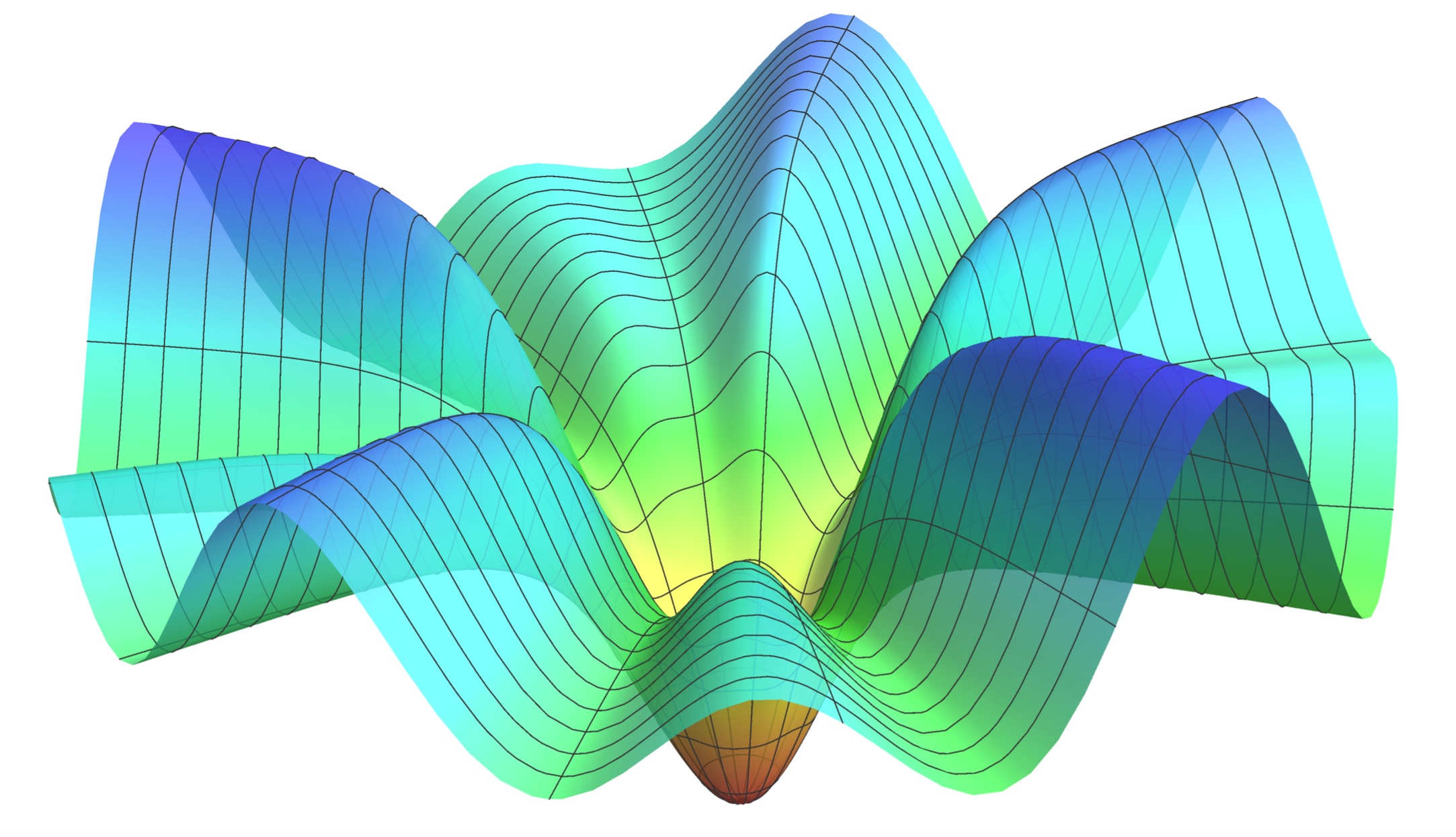
see Figure 1.

Later on, it was found [36] that one can strongly stabilize the field $\theta$ for all $\alpha$ and reduce investigation of the cosmological evolution to the study of the single inflaton field in the models with a somewhat different Kähler potential,

$$K=-{3\alpha}\ln{1-Z\bar{Z}\over|1-Z^{2}|}+S\bar{S}\ ,$$

(9)

and superpotential

$$W=S\,f(Z)\ ,$$

(10)

which yields the same inflaton potential (7) for $\theta=0$.

This considerably simplifies investigation of inflationary models. An advantage of this Kähler potential is its manifest shift symmetry: it vanishes along the direction $Z=\bar{Z}$, corresponding to $\theta=0$.

The next step was the construction of the anti-D3 brane induced geometric inflationary models with arbitrary $\alpha$ with a stabilized field $\theta$ [11] (see also [37]). The Kähler  function is

$$\mathcal{G}=\ln|W_{0}|^{2}-{3\alpha}\ln{1-Z\bar{Z}\over|1-Z^{2}|}+S+\bar{S}+G_{S\bar{S}}(Z,\bar{Z})S\bar{S}\ ,$$

(11)

where the field $S$ is nilpotent, with the metric

$$G_{S\bar{S}}(Z,\bar{Z})={|W_{0}|^{2}\over{\bf V}(Z,\bar{Z})+3|W_{0}|^{2}}\ .$$

(12)

The bosonic part of the supergravity action is

$$g^{-1}{\cal L}=3\alpha{dZd\bar{Z}\over(1-Z\bar{Z})^{2}}-{\bf V}(Z,\bar{Z})\ .$$

(13)

Note that the $Z$-part of the Kähler  potential has the inflaton shift symmetry at $Z=\bar{Z}$, as was shown in [36]. The potential is

$${\bf V}(Z,\bar{Z})=V(Z,\bar{Z})+|F_{S}|^{2}-3|W_{0}|^{2}=V(Z,\bar{Z})+\Lambda\ .$$

(14)

Here, as in all models in [11], $V(Z,\bar{Z})$ is a function of $Z$ and $\bar{Z}$ which is regular at the boundary $Z\bar{Z}=1$ and which vanishes at the minimum at $Z=0$, so that

$${\bf V}(Z,\bar{Z})\Big|_{Z=0}=|F_{S}|^{2}-3|W_{0}|^{2}\equiv\Lambda\ .$$

(15)

The scale of supersymmetry breaking due to the nilpotent field $S$ is $e^{\mathcal{G}}\mathcal{G}_{S}\mathcal{G}^{S\bar{S}}\mathcal{G}_{\bar{S}}\big|_{Z=0}=|F_{S}|^{2}\ ,$ and the gravitino mass is $m^{2}_{3/2}\Big|_{Z=0}=|W_{0}|^{2}\ .$. The angular field in these models is heavy, by construction, inflation takes place at $Z=\bar{Z}$.

This formulation is valid for any $\alpha$. However, subsequent investigations have revived interest in the specific models with $3\alpha=1$ corresponding to the unit size disk [8], and in the possibility to describe models originating from merger of several unit size disks, which may lead to $\alpha$-attractors with $3\alpha=1,2,3,...,7$ [9, 10, 11]. It has been argued that these models provide some of the better motivated targets for the future B-mode searches. Therefore it would be interesting to revisit all versions of these models, including the original versions with light, non-stabilized fields $\theta$ [8], since such models may exhibit a greater degree of symmetry, as shown in Figure 1. It would be particularly interesting to find the corresponding generalization of the anti-D3 brane induced geometric inflationary models described above, applicable specifically to models with $3\alpha=1$.

We find this new formulation by returning to the original Kähler  frame with the axion shift symmetry, $K=-\ln(1-Z\bar{Z})$, instead of $K=-\ln{1-Z\bar{Z}\over|1-Z^{2}|}$. In this way the mass of the $\theta$-field will become light and we will have a two-field evolution on the disk of unit size $3\alpha=1$. The Kähler  function which provides the action

$$g^{-1}{\cal L}={dZd\bar{Z}\over(1-Z\bar{Z})^{2}}-V(Z,\bar{Z})-\Lambda$$

(16)

will be taken in the following form:

$$\mathcal{G}=\ln|W_{0}|^{2}-\ln(1-Z\bar{Z})+S+\bar{S}+G_{S\bar{S}}(Z,\bar{Z})S\bar{S}\ .$$

(17)

Here the metric of the nilpotent superfield is

$$G_{S\bar{S}}(Z,\bar{Z})={|W_{0}|^{2}\over(1-Z\bar{Z})\Big(|F_{S}|^{2}+V(Z,\bar{Z})\Big)+2|W_{0}|^{2}Z\bar{Z}}\ .$$

(18)

It is different from the simpler version of $G_{S\bar{S}}$ in Equation (12), but the Kähler  potential $-\ln(1-Z\bar{Z})$ as a function of $Z,\bar{Z}$ is simpler here. Moreover, the $Z$-part of the Kähler  potential has an axion shift symmetry, it is $\theta$-independent.

One can show that the expression for the scalar potential in this theory is given by

$${\bf V}(Z,\bar{Z})=V(Z,\bar{Z})+|F_{S}|^{2}-3|W_{0}|^{2}=V(Z,\bar{Z})+\Lambda\ .$$

(19)

This result is very similar to Equation (14). However, (14) correctly represents the inflaton potential only along the inflaton direction $Z=\bar{Z}$. The potential for general values $Z\not=\bar{Z}$ must be calculated by the standard supergravity methods. This complication usually is not important for us since during inflation one can stabilize the fields along the inflaton direction $Z=\bar{Z}$. Meanwhile in our new approach, equation (19) gives the full expression for ${\bf V}(Z,\bar{Z})$, which is valid for any $Z$ and $\bar{Z}$ on the disk. This is a very special feature of the new formulation, which is valid for $3\alpha=1$.

During inflation, one can safely ignore the tiny cosmological constant $\Lambda\sim 10^{{-120}}$, so the potential (19) is given by an arbitrary real function $V(Z,\bar{Z})$. In the simplest cases, where $V$ is a function of $Z\bar{Z}$, it does not depend on the angular variable $\theta$, just as the potential in the theory (3) (4) for $3\alpha=1$ shown in Figure 1. For more general potentials, $V$ may depend on $\theta$, and the potentials can be quite steep with respect to $\rho$ and $\theta$.

The key feature of this class of models, as well as of the models (3) (4) for $3\alpha=1$, is that they describe hyperbolic moduli space corresponding to the Kähler potential $K=-\ln(1-Z\bar{Z})$, with the metric of the type encountered in the description of an open universe, see Equation (23) below. As we will see, the slow roll regime is possible for these two classes of theories even for very steep potentials, because of the hyperbolic geometry of the moduli space.

Now we come to study inflation with the above theoretical construction. Our starting point is

$$g^{-1}{\cal L}={dZd\bar{Z}\over(1-Z\bar{Z})^{2}}-V(Z,\bar{Z})~.$$

(20)

The complex variable on the disk can be expressed as

$$Z=\rho\,e^{i\theta}~,$$

(21)

where $\rho$ is the radial field and $\theta$ is the angular field. In general, the potential $V(\rho,\theta)$ in these variables can be quite complicated and steep. For simplicity, in the following we assume the potential vanishes at the origin $Z=0$ and is monotonic along the radial direction of the unit disk³³ 3 We leave other interesting cases with non-monotonic potential, such as the Mexican hat potential, for future work [38]., i.e. $V_{\rho}\geq 0$. One natural possibility is $V_{\rho}\sim V_{\theta}/\rho\sim V$, which at first glance cannot yield sufficient inflation. However, the hyperbolic geometry of the moduli space makes slow roll inflation possible even if the potential is quite steep.

To see this, and to connect this to a more familiar canonical field $\varphi$ in $3\alpha=1$ attractor models where the $\tanh$ argument is $\varphi/\sqrt{6\alpha}$, we can use the following relation

$$\rho=\tanh{\varphi\over\sqrt{2}}\ .$$

(22)

Therefore, our cosmological models with geometric kinetic terms are based on the following Lagrangian of the axion-dilaton system

$$g^{-1}{\cal L}={1\over 2}(\partial\varphi)^{2}+{1\over 4}\sinh^{2}(\sqrt{2}\varphi)(\partial\theta)^{2}-V(\varphi,\theta)\ ,$$

(23)

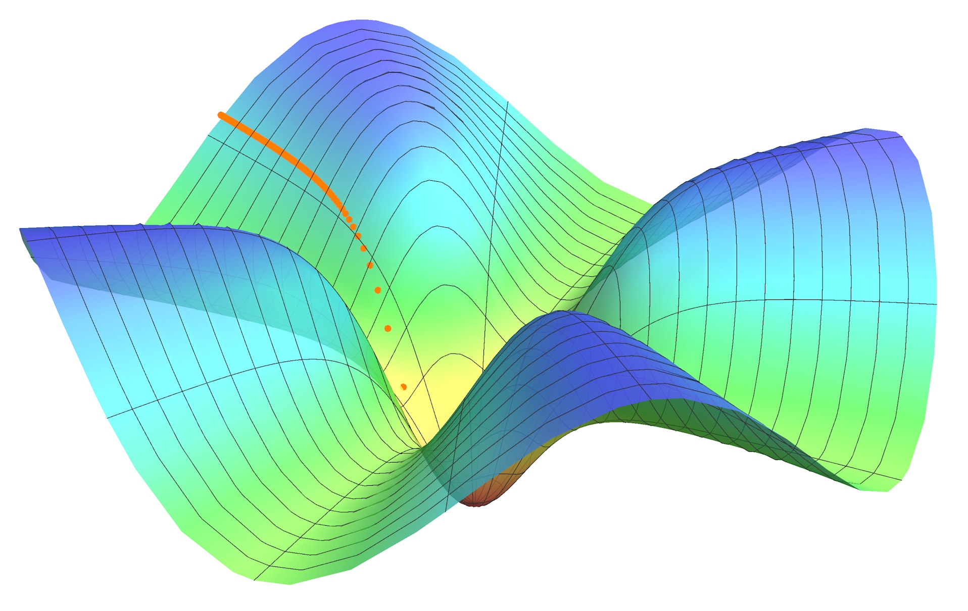
where some choice of the potentials $V(\varphi,\theta)$ will be made depending on both moduli fields. In terms of this new field $\varphi$, the corresponding potential near the boundary $\rho=1$ is exponentially stretched to form a plateau, where $\varphi$ field becomes light and slow-roll inflation naturally occurs. If we further assume the potential is a function of the radial field only, then we recover the T-model as shown in Figure 1. Generally speaking, the potential may also depend on $\theta$, and have ridges and valleys along the radial direction. One simple example is shown in Figure 2. Although the $\theta$ field can appear heavy in the unit disk coordinates, after stretching in the radial direction, the effective mass in the angular direction is also exponentially suppressed for $\varphi\gg 1$.

For a cosmological spacetime, the background dynamics is described by equations of motion of two scalar fields

$$\ddot{\varphi}+3H\dot{\varphi}+V_{\varphi}-\frac{1}{2\sqrt{2}}\sinh\left(2\sqrt{2}\varphi\right)\dot{\theta}^{2}=0~,$$

(24)

$$\ddot{\theta}+3H\dot{\theta}+\frac{V_{\theta}}{\frac{1}{2}\sinh^{2}(\sqrt{2}\varphi)}+\frac{2\dot{\theta}\dot{\varphi}}{\frac{1}{\sqrt{2}}\tanh(\sqrt{2}\varphi)}=0~,$$

(25)

and the Friedmann equation

$$3H^{2}={1\over 2}(\dot{\varphi}^{2}+{1\over 2}\sinh^{2}{{\sqrt{2}\varphi}}~\dot{\theta}^{2})+V(\varphi,\theta)\ ,$$

(26)

where $H\equiv\dot{a}/a$ is the Hubble parameter. In such a two-field system with potential as shown in Figure 2, one may expect that the inflaton will first roll down from the ridge to the valley, and then slowly rolls down to the minimum along the valley. In the following we will demonstrate, due to the magic of hyperbolic geometry, the dynamics of moduli fields is totally different from this naive picture.

One of the most important properties of single field $\alpha$-attractor inflation is the universal prediction for observations. For $\alpha\lesssim\mathcal{O}(1)$ and a broad class of potentials, as long as $V(\rho)$ is non-singular and rising near the boundary of the Poincaré disk, the resulting scalar tilt and tensor-to-scalar ratio converge to

$$n_{s}=1-\frac{2}{N}\quad\text{and}\quad r=\frac{12\alpha}{N^{2}},$$

(39)

where $N\sim 50-60$ is the number of e-folds for modes we observe in the CMB.

One interesting question is whether the universal predictions are still valid in the multi-field regime. In multi-field scenarios the curvature perturbation is sourced by the isocurvature modes on superhorizon scales, thus their evolution is typically non-trivial and yields totally different results for $n_{s}$ and $r$. As we show above, the angular dependence in the $\alpha$-attractor potentials indeed leads to multi-field evolution. For the toy model we studied, the behaviour of perturbations can be computed using the numerical code mTransport [39]. We focus on one single $k$ mode for curvature and isocurvature perturbations, and show their evolution in Figure 6. As expected, the curvature perturbation is enhanced during inflation, while the isocurvature modes decay. Therefore, naively one expects there would be corrections to the single field $\alpha$-attractor predictions due to the multi-field effects.

In the following we will show that, surprisingly, the universal predictions are still valid in the multi-field regime. We use the $\delta N$ formalism to derive the inflationary predictions for the multi-field $\alpha$-attractor models studied in this paper. A full analysis of the perturbations is left for Appendix B, where the evolution of the coupled system of curvature and isocurvature modes is solved via the first principle calculation .

The $\delta N$ formalism [40, 41, 42, 43, 44] is an intuitive and simple approach to solve for the curvature perturbation in multi-field models. At the end of inflation, regardless of the various field trajectories, the amplitude of curvature perturbations is only determined by the perturbation of the e-folding number $N$, which is caused by the initial field fluctuations. Therefore, without studying details of the coupled system of curvature and isocurvature modes, as long as we know how the number of e-foldings $N$ depends on the initial value of the two fields, the curvature perturbation can be calculated.

Let us therefore consider how the initial $\varphi$ and $\theta$ determine $N$. In this paper, we define the e-folding number as the one counted backwards from the end of inflation, thus $dN=-Hdt$. In terms of $N$, the slow-roll equation (30) becomes

$$\frac{d\varphi}{dN}\simeq 2\sqrt{2}e^{-\sqrt{2}\varphi}\frac{V_{\rho}}{V}~.$$

(40)

Since in the large $\varphi$ regime $\rho\rightarrow 1$ and $V_{\rho}/V$ is nearly constant for a given trajectory, the equation above yields the e-foldings from the end of inflation as

$$N=\frac{1}{B}e^{\sqrt{2}\varphi}+C(\theta)~,$$

(41)

where $B\equiv 4V_{\rho}/V$ and $C(\theta)$ is an $\mathcal{O}(1)$ integration constant which can be fixed by setting $N=0$ at the end of inflation. Thus, both two fields affect the duration of inflation as expected in multi-field models. By this expression, we can use the $\delta N$ formalism to find curvature perturbation at the end of inflation

$$\zeta=\delta N=\frac{\partial N}{\partial\varphi}\delta\varphi+\frac{\partial N}{\partial\theta}\delta\theta=\frac{\sqrt{2}e^{\sqrt{2}\varphi}}{B}\delta\varphi+\left(C_{\theta}-\frac{B_{\theta}}{B^{2}}e^{\sqrt{2}\varphi}\right)\delta\theta~.$$

(42)

As we see here, $\frac{\partial N}{\partial\varphi}$ and $\frac{\partial N}{\partial\theta}$ can be comparable to each other. However, one should keep in mind that $\theta$ field is non-canonical, thus to estimate the field fluctuation amplitudes at horizon-exit, one should consider the canonically normalized ones: $\delta\varphi$ and $\frac{1}{\sqrt{2}}\sinh(\sqrt{2}\varphi)\delta\theta$. Approximately in the large-$\varphi$ region we have the following relation

$$\delta\varphi\simeq\frac{e^{\sqrt{2}\varphi}}{2\sqrt{2}}\delta\theta\simeq\frac{H}{2\pi}~.$$

(43)

From here, we find that the field fluctuation $\delta\theta$ is exponentially suppressed, compared to the one from $\delta\varphi$. So we only need to take into account the first term in equation (42). In addition, equation (32) yields $\epsilon_{\varphi}=B^{2}e^{-2\sqrt{2}\varphi}/4$, which further simplifies the $\delta N$ formula to $\zeta\simeq\delta\varphi/\sqrt{2\epsilon_{\varphi}}$. In the end, the power spectrum of curvature perturbation can be expressed as

$$P_{\zeta}\equiv\frac{k^{3}}{2\pi^{2}}{|\zeta_{k}|}^{2}\simeq\frac{H^{2}}{8\pi^{2}\epsilon_{\varphi}}~.$$

(44)

It is interesting to note that this result does not depend on any parameters related to the multi-field effects (such as $\gamma$). Using (32) and (41), we also get $\epsilon_{\varphi}\simeq 1/(4N^{2})$, which has the same behaviour with the single-field potential slow-roll parameter $\epsilon_{V}$. Thus the power spectrum above is coincident with the single-field one. Then the predictions of scalar tilt and tensor-to-scalar ratio follow directly

$$n_{s}-1\simeq-\frac{2}{N}\quad\text{and}\quad r\simeq\frac{4}{N^{2}}~.$$

(45)

These results are further confirmed by solving the full evolution of perturbations as shown in Appendix B.

The $\delta N$ calculation above also demonstrates the counter-intuitive properties of multi-field $\alpha$-attractors. As we show in Section 3, the stretching effects of hyperbolic geometry not only flattens the potential in the radial direction, but also suppresses the angular velocity $\dot{\theta}$. At the level of perturbations, the similar effect occurs to the field fluctuations in the angular direction. While the canonically normalized angular field fluctuation has the same amplitude with $\delta\varphi$, the original field perturbation $\delta\theta$ is exponentially suppressed. Therefore, only the radial field fluctuation $\delta\varphi$ contributes to the final result.

Furthermore, the above results do not depend on the initial values of $\theta$, which correspond to different field trajectories as shown in Figure 3. Certainly their respective e-folding number $N$ and $\epsilon_{\varphi}$ can be different from each other. However, the $N$-dependence of $\epsilon_{\varphi}$ is the same for all the "rolling on the ridge" trajectories. Thus regardless of various initial values of $\theta$, the multi-field $\alpha$-attractors yield the same universal predictions for $n_{s}$ and $r$.

Typically, another prediction in multi-field inflation is large local non-Gaussianity, which is disfavoured by the latest data [2]. Therefore it is also worthwhile to estimate the size of the bispectrum in our model. Here we expand the $\delta N$ formula to the second order in field fluctuations

$$\zeta=\delta N=\frac{\partial N}{\partial\varphi}\delta\varphi+\frac{\partial N}{\partial\theta}\delta\theta+\frac{1}{2}\frac{\partial^{2}N}{\partial\varphi^{2}}\delta\varphi^{2}+\frac{1}{2}\frac{\partial^{2}N}{\partial\theta^{2}}\delta\theta^{2}+\frac{\partial^{2}N}{\partial\theta\partial\varphi}\delta\theta\delta\varphi~.$$

(46)

In principle, there are two contributions here: one captured by the $\delta N$ expansion, and another one caused by field interactions of $\delta\varphi$ and $\delta\theta$. However, for the same reason shown in (43), the $\delta\theta$-related terms in the expansion (46) are highly suppressed. Moreover, since there is no large coupling between field fluctuations, we expect that the second contribution to the bispectrum will also be negligible. As a result, the local non-Gaussianity is approximately given by $\delta\varphi$ terms in (46)

$$f_{\rm NL}\simeq\frac{5}{6}\left.\frac{\partial^{2}N}{\partial\varphi^{2}}\right/\left(\frac{\partial N}{\partial\varphi}\right)^{2}\simeq\frac{5}{6N}~,$$

(47)

which is coincident with the single field consistency relation $f_{\rm NL}=-\frac{5}{12}(n_{s}-1)$ [45, 46]. Again, we find the multi-field $\alpha$-attractor prediction returns to the single field one, which further demonstrates the scope of universality.

Our investigation was stimulated by the realization that $\alpha$-attractors have particularly interesting interpretation in supergravity models with $\alpha=1/3$. A significant deviation from $\alpha=1/3$ typically either makes the field $\theta$ tachyonic, or strongly stabilizes it at $\theta=0$, which results in a single-field inflation driven by the field $\varphi$, see e.g. (6). One may wonder, however, what happens if we consider a more general class of two-field $\alpha$-attractors, which may or may not have supergravity embedding, and concentrate on their general features related to the underlying hyperbolic geometry.

For general $\alpha$, the canonically normalized field in the radial direction is defined by $\rho=\tanh({\varphi/\sqrt{6\alpha}}$), which leads to the following kinetic term

$$\frac{1}{2}\left(\partial\varphi\right)^{2}+\frac{3\alpha}{4}\sinh^{2}\left(\sqrt{\frac{2}{3\alpha}}\varphi\right)\left(\partial\theta\right)^{2}.$$

(48)

The equations of motion (24) and (25) also change accordingly, see (57) and (58). Similarly as in Section 4, in the slow-roll and large-$\varphi$ approximations these equations reduce to

$$\frac{\dot{\theta}}{H}\simeq-\frac{8}{3\alpha}\frac{V_{\theta}}{V}e^{-2\sqrt{2\over{3\alpha}}\varphi}~,~~~~~~3H\dot{\varphi}\simeq-\frac{2\sqrt{2}}{\sqrt{3\alpha}}V_{\rho}e^{-\sqrt{2\over{3\alpha}}\varphi}~.$$

(49)

As we see, the angular motion is also exponentially suppressed, compared to the radial one. So the rolling on the ridge behaviour is not unique for $\alpha=1/3$, but quite general for any $\alpha\lesssim\mathcal{O}(1)$. Similarly to (34), we get the following condition to ensure its validity

$$\frac{V_{\rho}}{V}\gg\frac{4}{9\alpha}\left(\frac{V_{\theta}}{V}\right)^{2}e^{-\sqrt{2\over{3\alpha}}\varphi}~,$$

(50)

which can be satisfied easily by many choices of potential, generalizing the bound (34) to other values of $\alpha$. Therefore, the results follow directly just like we find in Section 3. For example, the ratio of proper velocities

$$\gamma=\frac{\sqrt{\frac{3\alpha}{2}}\sinh\left(\sqrt{\frac{2}{3\alpha}}\varphi\right)\dot{\theta}}{\dot{\varphi}}$$

(51)

is still nearly constant, while $\epsilon_{\varphi}$ evolves as

$$\epsilon_{\varphi}\simeq\frac{3\alpha}{4N^{2}}~.$$

(52)

Repeating the same $\delta N$ calculation for perturbations, we get $N\simeq 3\alpha e^{\sqrt{2/3\alpha}\varphi}/B$ and

$$\zeta=\delta N\simeq\frac{1}{\sqrt{2\epsilon_{\varphi}}}\delta\varphi,$$

(53)

which lead to the universal predictions (39) for generic $\alpha$. Therefore in a broader class of $\alpha$-attractors without supersymmetry, adding angular dependence to the potential will not modify the universal predictions either. Importantly, in order to validate the various assumptions we make to obtain the universal predictions, we need the potential to satisfy certain conditions. The most non-trivial condition is already given in (50). The additional constraints on the potential come from assuming the slow-roll, ‘slow-turn’ and large $\varphi$ approximation. We give more detail about these approximations and collect the constraints on the potential in Appendix A. Some of the conditions should also be satisfied for single field $\alpha$-attractors. The smaller $\alpha$ becomes, the more pronounced the stretching of the hyperbolic field metric gets and it will be more likely to be within the large $\varphi$ regime $\varphi\gtrsim\sqrt{\frac{3\alpha}{2}}$ and the slow-roll regime at the same time. Finally, there are some additional constraints on the potential because of the multi-field nature of our class of models. In particular, if we want to have suppressed field accelerations, we need to satisfy the slow-roll and the slow-turn conditions given in (59d) - (59f). A natural choice of the potential with $\frac{V_{\theta}}{\rho V}\sim\frac{V_{\rho}}{V}\sim\frac{V_{\theta\theta}}{\rho^{2}V}\sim\frac{V_{\theta\rho}}{\rho V}\sim\frac{V_{\rho\rho}}{V}\sim 1$, evaluated at the boundary $\rho\sim 1$ amply satisfies all conditions for $\alpha\lesssim O(1)$.

In this paper we have studied the inflationary dynamics and predictions of a class of $\alpha$-attractor models where both the radial and the angular component of the complex scalar field $Z=\rho\,e^{i\theta}$ are light during inflation. We concentrated on the special case $\alpha=1/3$, where the model has a supergravity embedding with a high degree of symmetry from $\mathcal{N}=4$ superconformal or $\mathcal{N}=8$ supergravity. However, our results may have more general validity under the conditions specified in Appendix A. Under the weak assumptions that the potential is monotonic in the radial coordinate, and the angular gradient is not exponentially larger than the radial gradient (34), we find exactly the same predictions as in the theory of the single field $\alpha$-attractors:

$$n_{s}-1\simeq-\frac{2}{N}\quad\text{and}\quad r\simeq\frac{12\alpha}{N^{2}}~.$$

(54)

Universality of these predictions may make it difficult to distinguish between different versions of $\alpha$-attractors by measuring $n_{s}$. However, from our perspective this universality is not a problem but an advantage of $\alpha$-attractors, resembling universality of several other general predictions of inflationary cosmology, such as the flatness, homogeneity and isotropy of the universe, and the flatness, adiabaticity and gaussianity of inflationary perturbations in single field inflationary models.

The hyperbolic field metric plays a key role in finding these universal results. Let us summarize how we arrived at our new result and stress how the hyperbolic geometry dictates the analysis.

• •

  First, the hyperbolic geometry effectively stretches and flattens the potential in the radial direction to a shape independent of the original radial potential. Independent - as long as the potential obeys the condition (34). The amplitude of this shape, however, varies along the angular direction.

• •

  Next, the angular velocity $\dot{\theta}$ is exponentially suppressed, due to the hyperbolic geometry, and inflation proceeds (almost) in the radial direction. The inflaton is "rolling on the ridge" in the $(\varphi,~\theta)$ plane. This is illustrated in Figures 3 and 4.

• •

  The straight radial trajectory is an illusion, since the physical velocity in the axion $\theta$ direction is typically of the same order as the radial velocity. The angle between the inflationary trajectory and the radial direction is nonzero and practically constant in this regime. Moreover, although the field is following the gradient flow, the trajectory is curved in the hyperbolic geometry. Therefore, the perturbations are coupled and the multi-field effects have to be taken into account.

• •

  Then, we use the $\delta N$ formalism to compute the power spectrum of curvature perturbations (confirmed by a fully multi-field analysis in Appendix B). The typical initial $\theta$ perturbations are very small and have a negligible effect on the number of efolds. However, the initial value of $\theta$ of a given trajectory determines how much a perturbation in the radial direction affects the number of efolds, since the trajectory is curved. At the same time the initial value of $\theta$ determines the renormalization of the slow-roll parameter $\epsilon$. These two effects cancel exactly, leaving us with the same predictions as the single field $\alpha$-attractors. Also the non-Gaussianity calculation recovers the single field result $f_{\rm NL}\simeq-\frac{5}{12}(n_{s}-1)$.

• •

  Finally, in Section 5 and Appendix A, we relax the condition $\alpha=1/3$ and simply assume the hyperbolic geometry (1) with smooth potentials. We identify the conditions on the potential in order to exhibit the universal behaviour discussed in our paper, see (59). For $\alpha\lesssim O(1)$ these conditions are amply satisfied by a broad class of potentials $V(\rho,\theta)$, including natural ones without a hierarchy of scales: $\frac{V_{\theta}}{\rho V}\sim\frac{V_{\rho}}{V}\sim\frac{V_{\theta\theta}}{\rho^{2}V}\sim\frac{V_{\theta\rho}}{\rho V}\sim\frac{V_{\rho\rho}}{V}\sim 1$, evaluated at the boundary $\rho\sim 1$.

In conclusion, the main result of our investigation is the stability of predictions of the cosmological $\alpha$-attractors with respect to significant modifications of the potential in terms of the original geometric variables $Z$. Whereas the stability with respect to the dependence of the potential on the radial component of the field $Z$ is well known [5], the stability with respect to the angular component of the field $Z$ is a novel result which we did not anticipate when we began this investigation.

Our results could have important implications for constructing UV completions of inflation. We have confirmed again that multi-field models of inflation can be perfectly compatible with the current data, in particular when the additional fields are very light. This lends support to the idea that it is not always necessary to stabilize all moduli fields in order to have a successful model of inflation.

Note added: After submission, Ref. [47] appeared, which provides a supergravity embedding for the more general $\alpha<1$ models discussed in Section 5.

References

- (1) Planck Collaboration, P. A. R. Ade et al., Planck 2015 results. XX. Constraints on inflation, arXiv:1502.02114.
- (2) Planck Collaboration, P. A. R. Ade et al., Planck 2015 results. XVII. Constraints on primordial non-Gaussianity, Astron. Astrophys. 594 (2016) A17, [arXiv:1502.01592].
- (3) R. Kallosh and A. Linde, Universality Class in Conformal Inflation, JCAP 1307 (2013) 002, [arXiv:1306.5220].
- (4) S. Ferrara, R. Kallosh, A. Linde, and M. Porrati, Minimal Supergravity Models of Inflation, Phys. Rev. D88 (2013), no. 8 085038, [arXiv:1307.7696].
- (5) R. Kallosh, A. Linde, and D. Roest, Superconformal Inflationary -Attractors, JHEP 11 (2013) 198, [arXiv:1311.0472].
- (6) S. Cecotti and R. Kallosh, Cosmological Attractor Models and Higher Curvature Supergravity, JHEP 05 (2014) 114, [arXiv:1403.2932].
- (7) M. Galante, R. Kallosh, A. Linde, and D. Roest, Unity of Cosmological Inflation Attractors, Phys. Rev. Lett. 114 (2015), no. 14 141302, [arXiv:1412.3797].
- (8) R. Kallosh and A. Linde, Escher in the Sky, Comptes Rendus Physique 16 (2015) 914–927, [arXiv:1503.06785].
- (9) S. Ferrara and R. Kallosh, Seven-Disk Manifold, -attractors and B-modes, arXiv:1610.04163.
- (10) R. Kallosh, A. Linde, T. Wrase, and Y. Yamada, Maximal Supersymmetry and B-Mode Targets, JHEP 04 (2017) 144, [arXiv:1704.04829].
- (11) R. Kallosh, A. Linde, D. Roest, and Y. Yamada, induced geometric inflation, JHEP 07 (2017) 057, [arXiv:1705.09247].
- (12) C. Gordon, D. Wands, B. A. Bassett, and R. Maartens, Adiabatic and entropy perturbations from inflation, Phys. Rev. D63 (2001) 023506, [astro-ph/0009131].
- (13) S. Groot Nibbelink and B. J. W. van Tent, Density perturbations arising from multiple field slow roll inflation, hep-ph/0011325.
- (14) S. Groot Nibbelink and B. J. W. van Tent, Scalar perturbations during multiple field slow-roll inflation, Class. Quant. Grav. 19 (2002) 613–640, [hep-ph/0107272].
- (15) N. Bartolo, S. Matarrese, and A. Riotto, Adiabatic and isocurvature perturbations from inflation: Power spectra and consistency relations, Phys. Rev. D64 (2001) 123504, [astro-ph/0107502].
- (16) Z. Lalak, D. Langlois, S. Pokorski, and K. Turzynski, Curvature and isocurvature perturbations in two-field inflation, JCAP 0707 (2007) 014, [arXiv:0704.0212].
- (17) A. Achucarro, J.-O. Gong, S. Hardeman, G. A. Palma, and S. P. Patil, Mass hierarchies and non-decoupling in multi-scalar field dynamics, Phys. Rev. D84 (2011) 043502, [arXiv:1005.3848].
- (18) A. Achucarro, J.-O. Gong, S. Hardeman, G. A. Palma, and S. P. Patil, Features of heavy physics in the CMB power spectrum, JCAP 1101 (2011) 030, [arXiv:1010.3693].
- (19) C. M. Peterson and M. Tegmark, Testing Two-Field Inflation, Phys. Rev. D83 (2011) 023522, [arXiv:1005.4056].
- (20) Y. Welling, Multiple Field Inflation and Signatures of Heavy Physics in the CMB, arXiv:1502.04369.
- (21) A. Achucarro, V. Atal, C. Germani, and G. A. Palma, Cumulative effects in inflation with ultra-light entropy modes, arXiv:1607.08609.
- (22) T. Kobayashi and S. Mukohyama, Effects of Light Fields During Inflation, Phys. Rev. D81 (2010) 103504, [arXiv:1003.0076].
- (23) S. Renaux-Petel and K. Turzynski, On reaching the adiabatic limit in multi-field inflation, JCAP 1506 (2015), no. 06 010, [arXiv:1405.6195].
- (24) S. Cremonini, Z. Lalak, and K. Turzynski, On Non-Canonical Kinetic Terms and the Tilt of the Power Spectrum, Phys. Rev. D82 (2010) 047301, [arXiv:1005.4347].
- (25) S. Cremonini, Z. Lalak, and K. Turzynski, Strongly Coupled Perturbations in Two-Field Inflationary Models, JCAP 1103 (2011) 016, [arXiv:1010.3021].
- (26) C. van de Bruck and M. Robinson, Power Spectra beyond the Slow Roll Approximation in Theories with Non-Canonical Kinetic Terms, JCAP 1408 (2014) 024, [arXiv:1404.7806].
- (27) R. Kallosh and A. Linde, Multi-field Conformal Cosmological Attractors, JCAP 1312 (2013) 006, [arXiv:1309.2015].
- (28) A. A. Starobinsky, S. Tsujikawa, and J. Yokoyama, Cosmological perturbations from multifield inflation in generalized Einstein theories, Nucl. Phys. B610 (2001) 383–410, [astro-ph/0107555].
- (29) F. Di Marco, F. Finelli, and R. Brandenberger, Adiabatic and isocurvature perturbations for multifield generalized Einstein models, Phys. Rev. D67 (2003) 063512, [astro-ph/0211276].
- (30) S. Renaux-Petel and K. Turzynski, Geometrical Destabilization of Inflation, Phys. Rev. Lett. 117 (2016), no. 14 141301, [arXiv:1510.01281].
- (31) J. Ellis, M. A. G. García, D. V. Nanopoulos, and K. A. Olive, Two-Field Analysis of No-Scale Supergravity Inflation, JCAP 1501 (2015) 010, [arXiv:1409.8197].
- (32) A. R. Brown, Hyperinflation, arXiv:1705.03023.
- (33) S. Mizuno and S. Mukohyama, Primordial perturbations from inflation with a hyperbolic field-space, arXiv:1707.05125.
- (34) A. Achucarro, O. Iarygina, G. Palma, V. Vardanyan, D.-G. Wang, and Y. Welling, In Preparation, .
- (35) S. Ferrara, R. Kallosh, and A. Linde, Cosmology with Nilpotent Superfields, JHEP 10 (2014) 143, [arXiv:1408.4096].
- (36) J. J. M. Carrasco, R. Kallosh, A. Linde, and D. Roest, Hyperbolic geometry of cosmological attractors, Phys. Rev. D92 (2015), no. 4 041301, [arXiv:1504.05557].
- (37) E. McDonough and M. Scalisi, Inflation from Nilpotent Kähler Corrections, JCAP 1611 (2016), no. 11 028, [arXiv:1609.00364].
- (38) A. Linde, D.-G. Wang, Y. Welling, Y. Yamada, and A. Achucarro, Hypernatural inflation, arXiv:1803.09911.
- (39) M. Dias, J. Frazer, and D. Seery, Computing observables in curved multifield models of inflation?A guide (with code) to the transport method, JCAP 1512 (2015), no. 12 030, [arXiv:1502.03125].
- (40) D. S. Salopek and J. R. Bond, Nonlinear evolution of long wavelength metric fluctuations in inflationary models, Phys. Rev. D42 (1990) 3936–3962.
- (41) M. Sasaki and E. D. Stewart, A General analytic formula for the spectral index of the density perturbations produced during inflation, Prog. Theor. Phys. 95 (1996) 71–78, [astro-ph/9507001].
- (42) A. A. Starobinsky, Multicomponent de Sitter (Inflationary) Stages and the Generation of Perturbations, JETP Lett. 42 (1985) 152–155. [Pisma Zh. Eksp. Teor. Fiz.42,124(1985)].
- (43) M. Sasaki and T. Tanaka, Superhorizon scale dynamics of multiscalar inflation, Prog. Theor. Phys. 99 (1998) 763–782, [gr-qc/9801017].
- (44) H.-C. Lee, M. Sasaki, E. D. Stewart, T. Tanaka, and S. Yokoyama, A New delta N formalism for multi-component inflation, JCAP 0510 (2005) 004, [astro-ph/0506262].
- (45) J. M. Maldacena, Non-Gaussian features of primordial fluctuations in single field inflationary models, JHEP 05 (2003) 013, [astro-ph/0210603].
- (46) P. Creminelli and M. Zaldarriaga, Single field consistency relation for the 3-point function, JCAP 0410 (2004) 006, [astro-ph/0407059].
- (47) Y. Yamada, U(1) symmetric -attractors, arXiv:1802.04848.