RSS Models for Respiration Rate Monitoring
Abstract
Received signal strength based respiration rate monitoring is emerging as an alternative non-contact technology. These systems make use of the radio measurements of short-range commodity wireless devices, which vary due to the inhalation and exhalation motion of a person. The success of respiration rate estimation using such measurements depends on the signal-to-noise ratio, which alters with properties of the person and with the measurement system. To date, no model has been presented that allows evaluation of different deployments or system configurations for successful breathing rate estimation. In this paper, a received signal strength model for respiration rate monitoring is introduced. It is shown that measurements in linear and logarithmic scale have the same functional form, and the same estimation techniques can be used in both cases. The implications of the model are validated under varying signal-to-noise ratio conditions using the performances of three estimators: batch frequency estimator, recursive Bayesian estimator, and model based estimator. The results are in coherence with the findings, and they imply that different estimators are advantageous in different signal-to-noise ratio regimes.
I Introduction
Serious respiratory disease can be identified by continuously monitoring variation of the respiration rate [1]. The importance of this vital sign is well acknowledged, and both contact and non-contact measurement systems are commercially available [2]. Non-contact respiration rate monitoring is advantageous compared to contact systems in terms of improved patient’s comfort and less patient distress, which result in improved accuracy. Although these devices fail to provide a measure to indicate actual respiratory gas-exchange [3], patient’s status can be attributed as stable or as at high-risk by continuously monitoring their respiration rate. In this paper, we consider non-contact respiration rate monitoring using commercially available low-cost standard wireless nodes. The main aim of these kind of systems is to estimate the respiration rate using the low-amplitude signal variations due to inhale and exhale motion.
The impact of respiration on the received signal has a complex relationship with the geometry and electrical properties of the objects in the environment, which is here referred to as the radio channel. As the granularity of the channel measurements increases, the information about the respiration can be better seen in the measurements. For example, high granularity measurements of different radar systems can be used for developing high quality monitoring systems [4, 5, 6]. However, higher quality channel measurements require complicated and expensive measurement systems. In contrast, monitoring systems based on commercially available narrowband communication systems are readily available, cheap, and easy to deploy. For example, several studies have evaluated the performance and different aspects of orthogonal-frequency-division-multiplexing (OFDM) based WiFi (IEEE 802.11 a, g, n, ac) [7], and low-power IEEE 802.15.4 compliant [8, 9, 10] systems. In this paper, narrowband and low-power systems, which provide received signal strength (RSS) measurements to assess the state of the propagation channel, are considered. Such measurements are the most challenging for breathing monitoring since their measurements provide only coarse information about the channel. However, it is possible to build very low-cost systems using off-the-shelf components or using already available radios of mobile devices or smart appliances.
Breathing monitoring using narrowband systems can be efficiently realized using a single pair of transmitter (TX) and receiver (RX) nodes [8]. The RSS measurements of the RX can be modeled as a single tone sinusoid contaminated with noise [9], whose maximum likelihood estimator using discrete time observations is known to be equivalent to the peak of discrete power spectral density of the measurements [11]. The estimation quality of such estimators, however, exhibits a thresholding behavior depending on the signal-to-noise ratio (SNR) of the measurements. When the SNR is low, the mean-square-error increases very rapidly and the estimation performance quickly degrades. To date, the SNR of RSS measurements for breathing rate monitoring has not been validated and no explanation of performance degradation has been provided. In this paper, a RSS model for respiration rate monitoring is presented, and its extensions for measurements in logarithmic scale and under quasi-linear movements are introduced. These allow one to predict the expected performance for a deployment scenario and patient position, and better assess the required system configuration for successful breathing monitoring.
In this paper, a RSS model of narrowband communication systems for respiration rate monitoring using the reflection based models is presented. The reflection model, previously explored for RSS-based localization [12, 13], is applied to respiration rate monitoring. Based on this model, first, it is shown that the breathing signal is frequency modulated into the RSS in linear scale due to small periodic movements. Such a signal exhibits relatively strong components on more than one frequency tones so that breathing estimators making use of this feature (see [14]) perform better in high SNR conditions. Then, it is also shown that the RSS in logarithmic scale also has the same form, and an explicit model is derived. The model itself allows us to evaluate feasibility of different breathing rate estimation techniques by enabling SNR evaluation of any given deployment. The impact of several parameters are evaluated both numerically and empirically. This paper makes the following contributions:
- •
A series expansion of the reflection-based RSS model is derived. This allows one to find several approximations to the observed RSS variations.
- •
A RSS model for small periodic perturbations (e.g. breathing motion) is derived. It is shown that the RSS variation due to such motions yields discrete tones at the harmonics of the perturbation frequency.
- •
A RSS model for small periodic perturbations when there is a linear movement is given. It is shown that the movement itself modulates the periodic perturbation, making the estimation a more challenging problem.
- •
Based on the models, various scenarios observed in empirical data are discussed and their impact on the observed RSS is shown.
- •
The performance of three different estimators are compared, and their performances are linked to the implications of the model.
The remaining part of the paper is organized as follows. First, the related work is summarized in Section II. The RSS measurement model and its series expansion are derived in Section III. The impact of small periodic movements and linear movements are derived, and various numerical evaluations are presented in the same section. Breathing rate estimation techniques are introduced in Section IV, before giving empirical evaluations in Section V. The conclusions are drawn in Section VI.
II Related Work
The importance of respiration rate has resulted in development of several respiration rate monitoring systems using different physical parameters (e.g. temperature, chest effort etc.) [2]. In this section, we only provide a brief review of radio-frequency based respiration rate monitoring methods, focusing on RSS-based approaches. The reader is referred to, for example, the works by AL-Khalidi et al. [2] and Folke et al. [3] for comprehensive technological overviews.
Respiration rate monitoring using radio frequency devices is a non-contact solution that has attracted significant attention. There are three different radar technologies that have been used for the purpose as has been reviewed by Li et al. [15]. The first work that appeared in the literature uses continuous wave (CW) Doppler radar system. Several studies have been published to analyze different aspect of similar systems, which can also estimate the heart rate along with respiration rate [16]. The impulse radio ultra wideband (IR-UWB) systems are also used for respiration rate monitoring [5]. They radiate and consume little power, may coexist well with other instruments, and perform better in environments with interference and severe multipath [17]. The characteristics of the received signal of IR-UWB systems were investigated by Venkatesh et al. [18]. However, these systems cannot cope with the impact of other motion or presence of more than one person [6]. Linear frequency modulated continuous wave (LFM-CW) systems can distinguish different reflector positions using their linearly varying frequency. This property has been used by Adib et al. for first estimating position of multiple persons in an environment [19], and then estimating the vital signs of each individual [6]. In this work, we show that indeed RSS has similar characteristics as the measurements of radar solutions, but require more carefully adjusted deployments.
The radar based solutions require a sophisticated hardware development for the vital sign monitoring. However, recent works on environmental sensing motivated RSS-based respiration rate monitoring using commodity wireless communication devices. The first work studying the feasibility of such systems makes use of multiple links formed by a mesh network of IEEE 802.15.4 nodes to estimate the breathing rate of a single person in the environment [9]. Later, this system was extended to estimate the location of a breathing person [10]. Several practical problems associated with the system are addressed in [8] by using only one pair of TX-RX nodes, detecting the moments breathing estimation is not possible, and using various signal processing techniques to improve SNR of the measurements. Due to widespread availability of WiFi, the communication channel measurements of these systems have also been used for respiration monitoring [7, 20]. The work by Abdelnasser et al. is based on the RSS measurements of WiFi systems [20]. On the other hand, the channel state information (CSI) output of OFDM-based WiFi radios provide higher granularity measurements of the communication channel, and have been used for vital sign monitoring purposes [21, 22, 23]. The CSI contains a complex channel gain estimate at each sub-carrier. In case the transmitted power is constant, the amplitude variation of these gains define the RSS variation at each sub-carrier in linear scale. Therefore, it can be argued that the RSS-based models and algorithms can be applied directly to CSI based systems that use amplitudes of the complex CSI vector components.
In this work, we model the RSS of narrowband communication systems for small periodic perturbations with unknown frequency, direction, and amplitude. It is shown that, similarly to signals in radar systems, the RF signal frequency modulate the periodic vital signals. The resultant model shows explicit relation between the respiration signal and initial position of the person, her orientation with respect to link-line, amplitude of the breathing, and the wavelength of the communication system. The SNR depends on these parameters as well as the noise power which dictates the performance of single tone parameter estimation techniques [11]. This result is coherent with empirical results of Luong et al. [24], real-time spectrum analyzer measurements in [8], and findings of Wang et al. [22]. The model also shows various interesting situations arising in practical deployments including the measurements showing only odd or even harmonics. It is further shown that the logarithmic transformation taking place in typical RSS measurement systems [25] does not change the signal type. Therefore, the developed model can be used for evaluating various deployment conditions that enable successful breathing rate monitoring.

III Received Signal Strength Models
In this section, we first review the RSS model, and then derive temporal variations of the RSS in linear scale for an object11 1 In this paper, we assume that the object is rigid so that any movement affects all points in its interior and on its boundary by the same amount. making movements in the form
| (1) |
where is a reference point at , is the constant velocity with amplitude for Euclidean norm , is the time elapsed since the epoch, is the low-amplitude movement displacement from the initial position and is the constant movement direction. We start with small perturbation case, where and small amplitude is periodic with frequency . Then, we include quasi-linear constant velocity movements characterized by . The obtained models are extended to RSS measurements systems that perform logarithmic transformations and show that the output of these systems have similar form as in the linear scale case.
III-A Background
For environmental sensing applications, the phenomenon of interest is estimated using the variation in RSS measurements compared to the measurement acquired when the object of interest is not in the medium, that is, the baseline RSS. A detailed analysis of the baseline RSS is provided in [25], and it is concluded that if the complex channel gain is constant, RSS is approximately a Gaussian random variable. This result also implies that if the medium is constant for the duration of acquiring the baseline RSS, their population mean converges to a constant due to the strong law of large numbers (SLLN). Then, the time average of the measurements also converges to the same constant since the channel is mean ergodic when the environment is static. In other words, the baseline RSS is given by
| (2) |
where is the signal-to-noise ratio (SNR) of the received signal under static channel conditions, and is the noise variance of the zero mean Gaussian noise in signal samples. Therefore, a practical measurement model for environmental sensing applications is
| (3) |
where is the channel gain when th RSS sample is acquired, and and is the constant channel gain of the baseline RSS. The last term is the joint noise process of all noise sources including white noise, round-off errors, quantization noise, and any source of uncertainty due to modeling errors, and its variance depends also on the current SNR value , which is time varying for the non-static case.
The expression in Eq. (3) implies that the complex channel gains and define the measurements. For the scenario visualized in Fig. 1, the ratio of channel gains22 2 The channel gain ratio follows from logarithmic scale definitions. If linear scale measurements are going to be used without calculating the amplitude ratio, the subsequent developments are valid through the relation , which has the same spectral properties as but with different DC term and amplitude scale. See Eq. (12) and its coefficients in Eq. (13). has already been investigated in [12, 13], and it has been shown that
| (4) |
where is excess path length traversed by the ray reflected from the object’s surface, is the effective reflection coefficient, denotes the wavelength, and we have dropped sample index from and . The effective reflection coefficient is defined as
| (5) |
where is the Fresnel reflection coefficient and is the path loss exponent modeling the fading experienced by both of the components [26, ch. 4]. The excess path length parametrizes the ellipse tangent to the interacting object at the point (cf. Fig. 1), and is defined as
| (6) |
for the symbols visualized on Fig. 1.
III-B Effect of Low Amplitude Periodic Perturbations
In the previous section, we analyzed the variation of RSS when the object abruptly appears in position which yield meters of excess path length when is the reflection point shown in Fig. 1. Now, suppose the object makes a time varying movement in a constant direction , that is, the reflection point moves to at time instant . At this new position, the excess path length can be found using its Taylor series expansion around as
where denotes the matrix transpose, is the gradient with respect to position , and we have used the fact that is a smooth function of both coordinates except at or . If the movement has a small amplitude , the second and higher order terms in the Taylor series expansion can be ignored, and one can write
| (7) |
where and we have explicitly written the gradient of with respect to at . Let us denote the inner product in Eq. (7) as
| (8) |
Then, Eq. (4) can be written as
| (9) |
It is to be noted that, for small amplitude perturbations satisfying , we have . Consequently, the frequency of the cosine term in Eq. (9) is defined by the perturbation amplitude , i.e., is a frequency modulated version of .
The amplitude ratio can be further simplified when is a periodic function33 3 The form of is selected for simplicity. The analysis can be straightforwardly extended to any periodic function using their Fourier series expansion as it is shown in [27, ch. 5].. Suppose that , so that the affective amplitude of the periodic movement , and constant phase can be defined as
| (10) |
Then, the Fourier series expansion of the cosine terms in Eq. (9) are given by
where is the Bessel function of the first kind [28, ch. 9]. Substituting this into Eq. (9) yields
| (11) |
which has the form of demodulated and low-pass filtered version of the respiration signal of IR-UWB systems derived by Venkatesh et al. [18].
Using the properties of Bessel function, the expression in Eq. (11) can be written in the form
| (12) | ||||
where coefficients are given by
| (13) |
III-C Effect of Quasi-linear Movements
Let us suppose that the object shown in Fig. 1 makes small periodic movements () in addition to a constant velocity movement in another direction so that at time instant , the initial point moves to If has a small amplitude and is close enough to the time epoch, the Taylor series expansion of the excess path length is valid, and for this case Eq. (7) can be written as
Similar to the definition in Eq. (8), let us denote the second inner product as
so that . Then, Eq. (4) becomes
| (14) | ||||
where the position dependence of and phase defined in Eq. (10), which cannot be ignored for this case, are explicitly written.
In case is a sinusoidal in the form , as in the previous subsection, then Eq. (14) can be written as
| (15) | ||||
Therefore, linear movements shift the frequency of the periodic movement and make the effective reflection coefficient defined in Eq. (5) a time varying quantity since term in cannot be neglected.
III-D RSS in Logarithmic Scale
Let us define the amplitude ratio in Eq. (4) in logarithmic scale as
| (16) | ||||
where is the base of the natural logarithm and we have defined
| (17) |
It can easily be verified that for so that and the power series expansion of the second term in Eq. (17) is given by
where the coefficients are given by
for all . In addition, the cosine powers can be expanded as harmonics,
where is an arbitrary argument of . Due to orthogonality of the sinusoidal functions, are polynomials of which can be written as
Note that for all , and for and we have . The partial sums of the coefficients are convergent, and after simplification and substituting definition of in Eq. (17) into this result yields
One important consequence is that is equal to the additive inverse of the first term in Eq. (16), and they cancel out. Therefore, the RSS measurement model in Eq. (16) can be written as
| (18) |
The series in Eq. (18) implies that the periodic sinusoidal perturbation in Eq. (11) after logarithmic transformation reads as
| (19) | ||||
where . Similarly, the impact of quasi-linear movement given in Eq. (15) for logarithmic scale is given by
| (20) | ||||
The series in Eq. (19) can be written in the form in Eq. (12),
| (21) | ||||
where, for this case, the coefficients are given by
| (22) |
Similar to Eq. (15), Eq. (20) can be written in the same form with coefficients in Eq. (22).

III-E Discussion
Suppose that the periodic movement represents respiration of a person, which is monitored by a TX-RX pair operating at ISM band so that . Although the respiration has a non-trivial relation between sex, age, and posture [29], on average, it is a small quantity, for example, maximum displacement44 4 This is an example value, and may not correspond to any specific combination of sex, age, and posture for a chest or abdominal movement associated with the respiration [29]. . An example deployment of such a system is expected to yield RSS measurements shown in Fig. 2.
A closer look at the coefficients in Eq. (22) reveals that when for any integer , all odd order harmonics get closer to due to product. Similarly, when for odd , all even order harmonics get closer to . Therefore, for some special values of initial excess path value , the breathing of a stationary person may exhibit only even or odd harmonics in their measurement signal. The same argument is true for RSS measurements in linear scale (see Eq. (13)), and it is independent of the actual periodic breathing signal function. In Fig. 2b, Eq. (16) is used for calculating the RSS values for different values. It can be seen that when , the RSS has a smaller amplitude but double perturbation frequency. At these distances, it can be observed from Fig. 3a that the signal energy is very small.
The respiration signal in Eq. (12) (and Eq. (21)), is series expansion of a frequency modulated signal. For frequency modulated signals, the number of terms in their series expansion can found by Carson’s bandwidth rule [27, ch. 5], which states that it is enough to consider only harmonics of the Fourier series in Eq. (11) and Eq. (15). Since the maximum displacement due to respiration can be assumed to satisfy , and its frequency can be assumed to be less than breaths per minute (), as it has been done earlier [9, 8], Carson’s rule imply that only two harmonics are needed to represent most of the signal. Consequently, a conservative approximation of the amplitude ratio in linear scale and in logarithmic scale is obtained by truncating the series in Eq. (12) at the second term. For lower respiration rates, it is possible to truncate the series after the first term and obtain a single tone approximation which was used in previous works [9].
The infinite series in Eq. (18) can be truncated at lower orders if the total signal energy is concentrated greatly in lower order harmonics. For this purpose, one can invoke Parseval’s Theorem to find the signal energy of from the periodic series expansion in Eq. (18) as
where is the di-logarithm function [30]. Then, the total signal power is monotonically increasing with . Since , defined in Eq. (5), is decreasing function of and increasing function of , it attains its maximum when so that . This implies that the signal energy concentrated at lower order harmonics if is lower than , which is defined by the incidence angle (cf. Fig. 1) and the object’s relative permittivity. When the reflector object is close to the link line, approaches to radians making very close to . In this case, high number of terms are needed to reach a good approximation of the series in Eq. (22). However, when the object is sufficiently far away from the link-line, assumes smaller values and increases, making a small quantity. When is smaller than , first two harmonics in Eq. (18) contain of total signal energy , making two term approximation a reasonable choice. The variation of root-mean-square error (RMSE) with excess path length is depicted in Fig. 2c for different truncation orders of the series in Eq. (22) while using only first two harmonics in Eq. (21). As shown, even for small , the two term series truncation yields small error.
The observed breathing signal amplitude depends on the effective amplitude of the breathing displacement defined in Eq. (), effective reflection coefficient defined in Eq. (5), and the excess path length when the person is in the initial position . The effect of position displacement on can be seen by inspecting its definition shown in Fig. 1, which yields
| (23) | ||||
Then, it follows from the definition of Fresnel reflection coefficient that its first order Taylor series expansion reads as
| (24) |
where is the coefficient at initial position , and is the relative permittivity. When the object is between the nodes, and as it gets closer to the link-line gets closer to , the rate of change of increases so that small amplitude perturbations may significantly alter .
Consider the signal energy of the approximate (two harmonics and two terms in coefficient series) signal, which is given by
| (25) |
Its variation with for the scenario used in generating the results in Fig. 2 is depicted in Fig. 3a. As shown, the energy may significantly change with the object’s position only. One consequence of this result is there are certain positions where small changes drastically degrades the SNR. For example, when the object in Fig. 2 is moving on the mid-line between TX and RX nodes, at certain -axis values, the relative importance of the second harmonic exceeds the first harmonic as shown in Fig. 3b. When excess path length is close to such a value, even small wavelength variations may change SNR of the measurements as can be observed from the dot plots in the figure. Furthermore, any uncertainty in electrical parameters of the object or its geometry increases the uncertainty further. Therefore, the SNR is statistical, and it is a very tedious task to accurately compare the model output with measurement data.
The analysis in the previous subsection and discussions above imply that:
- i.
- ii.
When the object moves even with a constant velocity, the perturbation spectrum shifts depending on the speed and direction of the movement. In this case, the perturbation frequency estimate has a different nature and it is required to first estimate the center frequency (see Eq. (20)). The other option is to stop estimating breathing rate when a movement is detected, as it has been done in [8].
- iii.
The signal energy can be estimated using Eq. (25) as the higher order terms introduce small modeling error.
- iv.
The breathing signal’s energy has a non-trivial relation with breathing direction with respect to the link-line, breathing amplitude, initial position of the person, her geometry, and electrical properties of her clothes. Therefore, the SNR of the breathing signal is statistical, and some diversity mechanism is needed to improve breathing estimation quality. For example in [8] frequency diversity and in [9] spatial diversity are used. In works using CSI output of WiFi devices, the channel gains are estimated for large number of subcarriers, which yields improved breathing rate estimation quality.
IV Breathing Rate Estimation
The analysis in the previous section conclude that the effect of respiration on RSS can be modeled in terms of the amplitude ratio in linear scale defined in Eq. (4) and in logarithmic scale defined in Eq. (16) along with the additive noise as shown in Fig. 4a.
In this section, we discuss three approaches to estimate the respiration rate . The estimators given in this section do not use the RSS measurements directly, but its bandpass filtered version or low-pass filtered , denoted as . These processing steps are visualized in Fig. 4b. The breathing rate estimation problem can be casted as single tone parameter estimation of a deterministic sinusoid using discrete observations as has been done in the related works [8, 10, 9]. The problem has been extensively studied due to its importance in various application areas [31, ch. 13]. In the first subsection, we give an overview of the batch-based frequency estimation technique. Then, we discuss a Bayesian formulation of the same approach, and summarize its recursive solution from the work by Qi et al. [32]. Finally, we review a recently introduced model-based approach [14].
IV-A Batch Spectral Analysis
The most straight forward and standard approach in the literature is to use spectral analysis using a batch of measurement data. It is well established that the maximum likelihood estimate of the frequency of an unknown sinusoid is the frequency of the peak of the periodogram [11]. The peak of the periodogram can be calculated using the fast Fourier transform (FFT). However, this method requires significant frequency resolution and high SNR for good performance since it is subject to thresholding effects. Here, we summarize the DFT-based method in a practical perspective.
For the DFT-based method, the maximum and minimum breathing rates (perturbation frequencies) can be used for bandpass filtering the measurements as shown in Fig. 4b. Then, the output signal is split into windows of length with overlap such that the data for the th window (for ) is given by
| (26) |
where the offset . Then, from Eq. (26), the power spectral density (PSD) is estimated as
| (27) |
where is the DFT of and the th frequency is given by
| (28) |
for and where is the sampling frequency.
Eq. (27) naturally yields the whole spectrum for all frequencies . In order to obtain a point estimate , the frequency corresponding to the maximum of the PSD is chosen, that is
| (29) |
excluding the DC component.
IV-B Recursive Bayesian Spectral Analysis
Rather than processing entire overlapping windows at a time, the spectrum can also be estimated by using a recursive Bayesian spectrum estimation approach [32]. This method can cope with the DC term since it is possible to choose the resolution and sampling rate. However, once these parameters are selected, the measurements must be low-pass filtered in order to keep the dimension of the state low. In other words, low-pass filtered RSS data (see Fig. 4b) can be used for estimating the perturbation frequency.
The Bayesian recursive method starts with writing in terms of its Fourier series expansion as
| (30) | ||||
where is the number of frequency bins, , , and are the time-varying Fourier coefficients with slight abuse of notation, are the frequency bins, and is the measurement noise which is a filtered version of , but still assumed to be white.
Let be the vector of the Fourier coefficients, which are assumed to evolve as a Gaussian random walk according to
| (31) |
where is the process noise with covariance matrix . Furthermore, assume that the initial state is distributed according to .
Combining Eq. (30) and Eq. (31), the following linear state space model is obtained
| (32a) | ||||
| (32b) | ||||
where is the identity matrix and is the dimensional observation matrix with the th component defined as
The linear model in Eq. (32) can then be used in a Kalman filter [33] to obtain recursive estimates of the Fourier coefficients at each time . Finally, a point estimate of the breathing frequency is obtained in the same way as for the spectrum based method, that is, by selecting the frequency with highest magnitude such that
| (33) |
Note that this method has all the advantages of recursive implementations including decreased computational and memory requirements. In addition to these, an important advantage of this method compared to the DFT-based approach is its capability of working with unevenly sampled data.
IV-C Model-based Estimation
In principle, the model of the RSS measurements in Eq. (12) and Eq. (21) could be exploited to improve the perturbation frequency estimation or to relax the requirements of the DFT based (both batch or recursive) estimators. However, since the small perturbations depend on many different parameters such as the breathing direction with respect to link-line, breathing amplitude, initial position of the person, their geometry, and electrical properties of their clothes this is non-trivial. Instead, non-parametric statistical models can be used for capturing these effects. This approach has recently been used in [14] by modeling the underlying signal as a quasi-periodic Gaussian process. Here, we just summarize the main results of this model-based method, and the reader is referred to [14] for related discussions and a detailed derivation.
The low-pass filtered RSS (see Fig. 4b) can be modeled as a quasi-periodic Gaussian process [34, 35], such that
| (34a) | ||||
| (34b) | ||||
where is the th sample acquired at time , and denotes a Gaussian process prior with mean function and covariance kernel , and [34]. For a temporal Gaussian process with the canonical periodic covariance function given by
| (35) |
it can be shown that the following equivalent discrete-time state-space formulation
| (36a) | ||||
| (36b) | ||||
| (36c) | ||||
can be obtained [35, 14]. In Eq. (35) (variance), (length scale), and (perturbation frequency) are hyperparameters. In Eq. (36), is the DC component, (for ) is a vector containing the instantaneous value of the harmonic and its derivative, and are the corresponding process noises, and
| (37a) | ||||
| (37b) | ||||
| (37c) | ||||
| (37d) | ||||
where is the th order modified Bessel function of the first kind, and . The initial states are given by and .
Additionally, the logarithm of the breathing frequency is modeled as a geometric Brownian motion which yields [36]
| (38) |
where is the spectral density of the underlying white noise process and .By introducing a time-varying frequency as in Eq. (38), this assumption is violated for the covariance kernel in Eq. (35). However, since the breathing rate varies relatively slowly, the process is considered locally stationary.
Finally, combining Equations (34), (36), and (38), and truncating the series in Eq. (36c) at some upper bound , the following nonlinear state-space model is obtained
| (39a) | ||||
| (39b) | ||||
where the dependence of the matrices on is implicit. The model Eq. (39) can now readily be used in a (nonlinear) Kalman filter such as the unscented Kalman filter or extended Kalman filter [33]. In this paper, we use Rao–Blackwellized unscented Kalman Filter presented earlier in [14]. Finally, the frequency estimate is given by
| (40) |
where is the first component of the latest state estimate.

| Symbol | Value | Appearance | Explanation |
| Varying | Sec. V-A | Breathing frequency in bpm | |
| Varying | Sec. V-A | Sampling frequency in Hz | |
| Eq. (27) | Number of FFT points | ||
| s data | Eq. (26) | FFT window length | |
| Eq. (26) | FFT window overlap | ||
| Eq. (30) | Number of frequency bins in KF | ||
| Eq. (32) | Process noise covariance | ||
| Eq. (32) | Initial estimate of KF | ||
| Eq. (32) | Covariance of the initial estimate | ||
| Eq. (30) | GP Truncation Order | ||
| Eq. (35) | Covariance kernel variance | ||
| Eq. (35) | Covariance kernel length scale | ||
| Eq. (38) | White noise process PSD | ||
| Eq. (37) | Time difference between samples in seconds | ||
| Eq. (37) | Covariance of the initial state estimate components corresponding to DC terms | ||
| Eq. (37) | Covariance of the initial state estimate components corresponding to non-DC terms | ||
| Eq. (39) | Initial estimate of GP | ||
| Various | Measurement noise variance for KF and GP models |
V Experimental Results
In this section, the developments of the paper are evaluated using experimental data. In the following, we present the experimental setup and overview of the experiments before introducing the evaluation metrics. Then, the results are given.
V-A Experimental Setup and Experiments
The experiments are conducted using the nodes with the hardware and software platform described in [37]. A TX node is programmed to transmit packets over frequency channels at the GHz ISM band55 5 The developments presented thus far consider a stream of RSS measurements with constant wavelength. In this section, the acquired measurements from different frequency channels are considered as different measurements with different wavelengths.. After each transmission, the frequency channel of communication is changed sequentially to cover the MHz spectrum. The RX nodes are programmed to listen for ongoing transmissions. Upon reception, the packets are timestamped at the start of frame delimiter with a resolution of microseconds, and the received frames are stored to a non-volatile memory.
The first experiment aims at evaluating the accuracy of the estimators and the experimental procedure follows that of experiment no. 1 in [8]. The RSS measurements are acquired by a single RX node, which is away form the TX node. The transmission interval is set to . Thus, for each frequency channel, which is considerably higher than the breathing frequencies of interest. During the experiments the person is lying on a bed, where his chest is approximately away from the link-line while breathing at a constant rate set by a metronome. The person breaths at different rates: breaths-per-minute (bpm). In total time series are recorded and used for evaluation purposes. We refer to this experiment as bed experiment.
The second experiment aims at evaluating how the SNR impacts estimation performance. The TX node emits frames every , and RX nodes acquire the RSS variation when the person is standing in four different positions as shown in Fig. 6a. At each position, the person is standing still while breathing at a constant rate of bpm. The setup is also used for acquiring RSS measurements when the environment is empty. In total time series are recorded for each position so that the evaluation is based on data series. We refer to this experiment as room experiment.
The acquired RSS data is preprocessed as shown in Fig. 4b. The bandpass filtered data is obtained as output of two processing stages: first the mean is calculated and removed from measurement , and then the result is low-pass filtered. The low-pass filtered data is obtained by just low-pass filtering . The used low pass filter is a th order elliptic filter that has passband frequency of and stop frequency of , maximum ripple in the pass band, and stop band attenuation.
V-B Evaluation Methodology
During the evaluation, we refer to the output of the batch estimator summarized in Sec. IV-A as DFT estimate, the recursive Bayesian estimator presented in Sec. IV-B as Kalman Filter (KF) estimate, and finally, the model-based estimator presented in Sec. IV-C output is referred to as Gaussian Process (GP) estimate. These methods are implemented using the parameters tabulated in Table I.
The evaluation in this section is based on mean absolute error (MAE) calculations. For the breathing frequency estimation, the MAE in bpm is defined as
| (41) |
where is the true rate, and is the th frequency estimate out of total estimates. This metric fails to provide a measure of dispersion in the estimates. For this purpose, we use the ratio of estimates within bpm neighborhood of the true frequency
| (42) |
In order to quantify the convergence speed of the methods, we calculate for the data in the first and for the data afterwards separately. We refer to the former as and the latter as . When the estimates have some outliers, e.g. they converge to the second harmonic frequency, we also calculate by excluding those outliers, and refer the result with w/o outliers.
In high SNR conditions, the performance of all the estimators are similar. In this case, the MAE of the estimated signal and the estimator input can be used for evaluation, since the estimator outputs also imply a signal in a specific form. Let us denote the model output of any estimator66 6 Although the state space models in Sec. IV are different, all of these yield the same output form as in Eq. (21) only with different number of harmonics. as . Then, we define the modeling MAE as
| (43) |
where for DFT-based method we add the mean value subtracted in the preprocessing stage.
The room experiment is used for evaluating the performance of the estimators under varying SNR conditions. The SNR of the signal is estimated using the PSD estimate in Eq. (27), using the actual breathing frequency. Let set contain the indices of the bins that are in a neighborhood of the harmonics of the true breathing frequency, excluding the DC term, and denote the bins within interval and Hz, which define the frequency range we are interested in. Then, an SNR estimate is given by
| (44) |
where the sets are disjoint. In the following, we use only the first two harmonics when forming the set , and all other spectral bins contribute to the noise power.
V-C Results
V-C1 Bed experiment
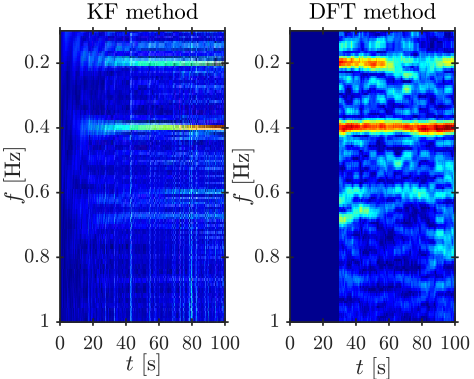
In Fig. 5, breathing estimation is illustrated on two different frequency channels when the person is breathing at a constant rate of , that is, . The signal shown in Fig. 5a contains a strong first harmonic at the breathing frequency and all methods are capable of estimating the true frequency correctly as illustrated in Fig. 5d. The recursive GP and KF methods converge to the true frequency in approximately , whereas the DFT method requires because of the time window used to calculate the DFT. The breathing induced changes are not as evident for the signal shown in Fig. 5e since it contains higher order harmonics as proposed by the model and as illustrated in Fig. 5g. The KF and DFT methods estimate the breathing frequency using the peak of the spectrum, resulting in an incorrect estimate of which corresponds to the second harmonic. The higher order harmonics are taken into account in the GP-based estimator when truncation order is higher than , . As a result, the method can correctly estimate the true breathing frequency as illustrated in Fig. 5h. The state estimates of the GP are illustrated in Fig. 5f and clearly, the method is able to track the DC-component and the harmonics accurately resulting in an improvement with respect to the spectral estimation techniques. For clarity, the second component of is omitted from Figs. 5b and 5f.
| GP | KF | DFT | |
|---|---|---|---|
| [%] | 97.50 | 88.75 | 87.50 |
| [bpm] | 1.06 | 5.10 | - |
| [bpm] | 0.25 | 1.44 | 1.41 |
| w/o outliers [bpm] | 0.15 | 0.25 | 0.26 |
| [dB] | 0.16 | 0.32 | 0.28 |
The measurement setup of the bed experiment is a realization of the measurement setup evaluated in Fig. 3b. Thus, small displacements of the person, as can be observed in Fig. 3b, causes drastic changes in the SNR. Furthermore, different frequency channel measurements may have different behavior as the spread of the dots in the figure imply. For the acquired signals, there are signals having higher energy in the second harmonic. According to the evaluation in Fig. 3b, a particular value (between and m) can yield such measurements. Therefore, the model correctly resembles this important scenario.
Performance of the estimators is summarized in Table II and on average, the spectral estimation techniques yield comparative accuracy while the GP-based estimator outperforms them. The ratio of valid estimates is summarized by and the difference in favor of the GP method originates from the fact that the second harmonic has the highest amplitude in out of signals resulting incorrect estimates with the spectral techniques. The recursive GP and KF methods typically converge in the first and of the estimates converge to within of the true rate in with GP and in with KF. However, the GP attains a significantly lower compared to KF, since the KF errors are typically very large due to the jumpy behavior as observed in Fig. 5d. After the transient period , the GP achieves a lower MAE than the spectral estimation techniques as given by . However, these results are severely affected by the experiments that resulted in incorrect estimates due to measurements not showing the first harmonic, but the second one. Neglecting these outliers, one can observe that all methods yield comparative accuracy as given in the fifth row of Table II. The steady-state accuracy of the spectral methods is mainly affected by the frequency bin size, whereas the GP accuracy could be improved by selecting the spectral density smaller. However, this would also decrease responsiveness of the filter to possible breathing rate changes. Lastly, is given in the last row of Table II. Clearly, the GP model estimates correspond more closely to the measured RSS since the higher order harmonics are taken into account.
The development in Sec. III concludes that the RSS is composed of more than one harmonics. However, the relative importance of higher order harmonics depend on several factors, which include actual breathing function (in this regard it is evident that natural breathing is not a sinusoid) and effect of quantization in typical RSS measurement systems [25]. In order to quantify the importance of higher order harmonics, one may investigate the estimated energy in harmonics for all time series.
| Truncation order | 1 | 2 | 3 | 4 |
|---|---|---|---|---|
| [%] | 97.50 | 97.50 | 97.50 | 97.50 |
| [bpm] | 0.28 | 0.29 | 0.25 | 0.25 |
| [dB] | 0.19 | 0.17 | 0.16 | 0.16 |
Since the model in Eq. (36c) is composed of Fourier series coefficients (and their derivatives), the relative energy in the th harmonic can be defined as
where denotes the first component of .
Averaging across the experiments results to , thus the first two harmonics contain approximately of the energy. This value is very close to the value predicted by the Carson’s rule of thumb, and implies that the actual breathing signal is a smooth function, not containing any jumps. Typically , but it can be as low as validating the importance of having an estimator that takes into account the higher harmonics. The accuracy of the GP with different truncation orders is given in Table III. In terms of estimation accuracy, higher truncation order yields slightly better performance as indicated by . In addition, is reduced with higher truncation order.
V-C2 Room experiment
CDFs of link SNRs for the room experiment are illustrated in Fig. 6b. The maximum SNR value for the empty room measurements is and of link SNRs exceeds this value when a breathing person is present. Thus, all positions clearly contain information regarding respiration rate of the person. However, SNR in the room experiments is typically much lower than in the bed experiment as shown in Fig. 6b.
| Receiver number | |||||||||||
| pos. | 1 | 2 | 3 | 4 | 5 | 6 | 7 | 8 | 9 | 10 | 11 |
| 1 | 6 | 0 | 13 | 0 | 6 | 19 | 19 | 19 | 25 | 19 | 6 |
| 2 | 0 | 6 | 75 | 44 | 13 | 31 | 6 | 6 | 38 | 6 | 13 |
| 3 | 0 | 0 | 6 | 6 | 25 | 13 | 6 | 25 | 6 | 6 | 25 |
| 4 | 0 | 0 | 0 | 6 | 19 | 0 | 13 | 0 | 6 | 0 | 31 |
The SNR of a link is defined by the signal energy given in Eq. (25) for which the coefficients can be calculated using Eq. (22). The coefficients are functions effective reflection coefficient , defined in Eq. (5), and effective amplitude of the periodic movement given in Eq. (10). The signal energy increases as increases, and has its maximum when is at its maximum on the link line. In the room experiment, when the person is on position , is in the interval for nodes to (), whereas for nodes , . As a result, the calculated signal energy for RX nodes and for nodes . With nodes , the average SNR is and whereas with RX nodes , the average SNR is and . Thus, in position , it is expected that successful breathing monitoring is more likely with nodes . The estimation results given in Table IV are in accordance with this statement.
The effective reflection coefficient is not the only parameter that affects the signal energy. In position , is in for nodes , whereas for nodes , . Respectively, the effective perturbation amplitude for nodes , it is in for . Position does not favor breathing monitoring using nodes despite that is three times larger than with nodes . The reason for this short coming is that breathing causes very small changes in the RSS of nodes and , whereas for nodes the signal energy is due to orientation of the person. Correspondingly, the average SNR of RS nodes is and , whereas for RX nodes the average SNR is and . Again, the experimental results support the implications of the model.
It is important to keep in mind that a slight change in position or orientation can have a significant impact on the signal energy of the links and therefore, spatial diversity or frequency channel diversity must be used to increase likelihood of successful breathing monitoring. Results for the different receivers and positions are summarized in Table IV and it can be concluded that successful breathing monitoring is very likely across a large area as long as the position and orientation of the person yield SNR higher than dB as in the bed experiment.
In Fig. 6c, the variation of as a function of SNR using the different estimators is depicted. As shown, estimation accuracy improves with every estimator when the SNR increases and with all methods when . Although for the bed experiment GP outperforms the other estimators, its performance is lower when the SNR is low. In this region, the second and higher order harmonics have lower power than the noise so that they are not as important as they are under high SNR conditions. Correspondingly, the batch DFT method and recursive spectral estimators outperform GP. This result suggests that for low SNR operating region batch DFT estimator is better whereas for high SNR conditions GP is better in terms of accuracy. It is also to be noted that GP has other advantages, most notably it relaxes data acquisition requirements by not requiring uniform sampling, operating with occasional packet losses, and better fusing the measurements from different communication channels [14]. Therefore, it has an utmost importance to investigate achievable performance, and to select an appropriate estimator.
VI Conclusions
Breathing rate is an important vital sign of which continuous monitoring may help to identify serious problems before they actually occur. In this paper, a signal model for received signal strength based non-contact respiration rate monitoring systems using commodity wireless devices is presented. It is shown that the signal model for low-end communication devices has the same form as the one in high-end radar based solutions. The effect of linear movement has also been derived, and significance of physical parameters are shown and discussed. Real world measurements are used for evaluating the performances of three previously presented estimators, and the result is compared with the implications of the model. The model implications are in coherence with the findings, and show that respiration rate monitoring systems must be evaluated before deployment. The estimator must be selected according to expected signal-to-noise ratio of the measurements and the constraints imposed by the hardware and software implementations of the wireless nodes.
References
- [1] M. A. Cretikos, R. Bellomo, K. Hillman, J. Chen, S. Finfer, and A. Flabouris, “Respiratory rate: the neglected vital sign,” Medical Journal of Australia, vol. 188, no. 11, p. 657, 2008.
- [2] F. Q. AL-Khalidi, R. Saatchi, D. Burke, H. Elphick, and S. Tan, “Respiration rate monitoring methods: A review,” Pediatric Pulmonology, vol. 46, no. 6, pp. 523–529, 2011.
- [3] M. Folke, L. Cernerud, M. Ekström, and B. Hök, “Critical review of non-invasive respiratory monitoring in medical care,” Medical and Biological Engineering and Computing, vol. 41, no. 4, pp. 377–383, 2003.
- [4] E. F. Greneker, “Radar sensing of heartbeat and respiration at a distance with security applications,” in Proceedings of Radar Sensor Technology II (SPIE 3066), vol. 3066. SPIE, 1997, pp. 22 – 27.
- [5] E. M. Staderini, “UWB radars in medicine,” IEEE Aerospace and Electronic Systems Magazine, vol. 17, no. 1, pp. 13–18, Jan 2002.
- [6] F. Adib, H. Mao, Z. Kabelac, D. Katabi, and R. C. Miller, “Smart homes that monitor breathing and heart rate,” in Proceedings of the 33rd Annual ACM Conference on Human Factors in Computing Systems, ser. CHI ’15. New York, NY, USA: ACM, 2015, pp. 837–846.
- [7] X. Liu, J. Cao, S. Tang, and J. Wen, “Wi-Sleep: Contactless sleep monitoring via WiFi signals,” in IEEE Real-Time Systems Symposium 2014, Dec 2014, pp. 346–355.
- [8] O. Kaltiokallio, H. Yiğitler, R. Jäntti, and N. Patwari, “Non-invasive respiration rate monitoring using a single COTS TX-RX pair,” in Proceedings of the 13th International Symposium on Information Processing in Sensor Networks, IPSN-14, April 2014, pp. 59–69.
- [9] N. Patwari, J. Wilson, S. Ananthanarayanan, S. K. Kasera, and D. R. Westenskow, “Monitoring breathing via signal strength in wireless networks,” IEEE Transactions on Mobile Computing, vol. 13, no. 8, pp. 1774–1786, 2014.
- [10] N. Patwari, L. Brewer, Q. Tate, O. Kaltiokallio, and M. Bocca, “Breathfinding: A wireless network that monitors and locates breathing in a home,” IEEE Journal of Selected Topics in Signal Processing, vol. 8, no. 1, pp. 30–42, Feb 2014.
- [11] D. Rife and R. Boorstyn, “Single tone parameter estimation from discrete-time observations,” IEEE Transactions on Information Theory, vol. 20, no. 5, pp. 591–598, 1974.
- [12] H. Yiğitler, R. Jäntti, O. Kaltiokallio, and N. Patwari, “Detector based radio tomographic imaging,” IEEE Transaction on Mobile Computing, vol. X, no. X, pp. PP–PP, XX 2017.
- [13] O. Kaltiokallio, H. Yiğitler, and R. Jäntti, “A three-state received signal strength model for device-free localization,” IEEE Transaction on Vehicular Technology, vol. X, no. X, pp. PP–PP, XX 2017.
- [14] R. Hostettler, O. Kaltiokallio, H. Yiğitler, S. Särkkä, and R. Jäntti, “RSS-based respiratory rate monitoring using periodic Gaussian processes and Kalman filtering,” in 25th European Signal Processing Conference (EUSIPCO), Kos, Greece, August 2017.
- [15] C. Li, V. M. Lubecke, O. Boric-Lubecke, and J. Lin, “A review on recent advances in doppler radar sensors for noncontact healthcare monitoring,” IEEE Transactions on Microwave Theory and Techniques, vol. 61, no. 5, pp. 2046–2060, May 2013.
- [16] J. Salmi, O. Luukkonen, and V. Koivunen, “Continuous wave radar based vital sign estimation: Modeling and experiments,” in IEEE Radar Conference (RADAR), 2012, 2012, pp. 0564–0569.
- [17] A. Lazaro, D. Girbau, and R. Villarino, “Analysis of vital signs monitoring using an ir-uwb radar,” Progress In Electromagnetics Research, vol. 100, pp. 265–284, 2010.
- [18] S. Venkatesh, C. R. Anderson, N. V. Rivera, and R. M. Buehrer, “Implementation and analysis of respiration-rate estimation using impulse-based UWB,” in IEEE Military Communications Conference, 2005. MILCOM 2005. IEEE, 2005, pp. 3314–3320.
- [19] F. Adib, Z. Kabelac, D. Katabi, and R. C. Miller, “3D tracking via body radio reflections.” in NSDI, vol. 14, 2014, pp. 317–329.
- [20] H. Abdelnasser, K. A. Harras, and M. Youssef, “UbiBreathe: A ubiquitous non-invasive WiFi-based breathing estimator,” in Proceedings of the 16th ACM International Symposium on Mobile Ad Hoc Networking and Computing. ACM, 2015, pp. 277–286.
- [21] J. Liu, Y. Wang, Y. Chen, J. Yang, X. Chen, and J. Cheng, “Tracking vital signs during sleep leveraging off-the-shelf WiFi,” in Proceedings of the 16th ACM International Symposium on Mobile Ad Hoc Networking and Computing. ACM, 2015, pp. 267–276.
- [22] H. Wang, D. Zhang, J. Ma, Y. Wang, Y. Wang, D. Wu, T. Gu, and B. Xie, “Human respiration detection with commodity WiFi devices: do user location and body orientation matter?” in Proceedings of the 2016 ACM International Joint Conference on Pervasive and Ubiquitous Computing. ACM, 2016, pp. 25–36.
- [23] X. Liu, J. Cao, S. Tang, J. Wen, and P. Guo, “Contactless respiration monitoring via off-the-shelf WiFi devices,” IEEE Transactions on Mobile Computing, vol. 15, no. 10, pp. 2466–2479, 2016.
- [24] A. Luong, A. S. Abrar, T. Schmid, and N. Patwari, “RSS step size: 1 dB is not enough!” in Proceedings of the 3rd Workshop on Hot Topics in Wireless. ACM, 2016, pp. 17–21.
- [25] H. Yiğitler, R. Jäntti, and N. Patwari, “On log-normality of RSSI in narrowband receivers under static conditions,” IEEE Signal Processing Letters, vol. 24, no. 4, pp. 367–371, April 2017.
- [26] T. S. Rappaport, Wireless Communications: Principles and Practice, 2nd ed. Prentice Hall, 2002.
- [27] A. B. Carlson, P. B. Crilly, and J. Ruttledge, Communication systems: An introduction to signals and noise in electrical communication, 4th ed. McGraw-Hill New York, 2002.
- [28] M. Abramowitz and I. A. Stegun, Handbook of mathematical functions: with formulas, graphs, and mathematical tables. Dover Publications, 1970.
- [29] H. Kaneko and J. Horie, “Breathing movements of the chest and abdominal wall in healthy subjects,” Respiratory Care, vol. 57, no. 9, pp. 1442–1451, 2012.
- [30] L. C. Maximon, “The dilogarithm function for complex argument,” Proceedings of the Royal Society of London. Series A: Mathematical, Physical and Engineering Sciences, vol. 459, no. 2039, pp. 2807–2819, 2003.
- [31] S. M. Kay, Modern Spectral Estimation. Prentice-Hall, 1988.
- [32] Y. Qi, T. P. Minka, and R. W. Picard, “Bayesian spectrum estimation of unevenly sampled nonstationary data,” in IEEE International Conference on Acoustics, Speech, and Signal Processing (ICASSP), vol. 2, May 2002, pp. 1473–1476.
- [33] S. Särkkä, A. Solin, and J. Hartikainen, “Spatiotemporal learning via infinite-dimensional Bayesian filtering and smoothing: A look at Gaussian process regression through Kalman filtering,” IEEE Signal Processing Magazine, vol. 30, no. 4, pp. 51–61, July 2013.
- [34] C. E. Rasmussen and C. K. I. Williams, Gaussian Processes for Machine Learning. MIT Press, 2006.
- [35] A. Solin and S. Särkkä, “Explicit link between periodic covariance functions and state space models,” in Proceedings of the 17th International Conference on Artificial Intelligence and Statistics (AISTATS), vol. 33, 2014, pp. 904–912.
- [36] B. Øksendal, Stochastic Differential Equations: An Introduction with Applications, 6th ed. Springer, 2010.
- [37] H. Yiğitler, R. Jäntti, and R. Virrankoski, “pRoot: An adaptable wireless sensor-actuator hardware platform,” in 12th IEEE International Conference on Embedded and Ubiquitous Computing (EUC). IEEE, 2014, pp. 281–286.