Calibration Concordance for Astronomical Instruments
via Multiplicative ShrinkageThanks: Herman Marshall is Astrophysicist, MIT Kavli Institute, Cambridge, MA 02139.Thanks: Vinay Kashyap is Astrophysicist, Harvard-Smithsonian Center for Astrophysics, Cambridge, MA 02138.

In astrophysics, various instruments such as telescopes are used by different teams of scientists to understand intrinsic properties of astronomical objects, i.e., sources such as stars. Although it is possible to make relative comparisons of different sources observed with the same instrument, unless the instruments are properly calibrated (Sembay et al.,, 2010), we cannot make reliable absolute measurements or make comparisons of sources observed with different instruments. Therefore, calibration of different instruments is an important, and on-going, problem for astrophysicists (Seward,, 1992; Matthews and Havey,, 2010; Nevalainen et al.,, 2010; Tsujimoto et al.,, 2011; Read et al.,, 2014; Schellenberger et al.,, 2015; Madsen et al.,, 2016, e.g.,).

As an example, space-based (e.g., X-ray) telescope calibration (Schwartz,, 2014) is handled in two phases: first, under controlled laboratory conditions (“ground” calibration), and second, while in space using astrophysical sources (“in-flight” calibration; see Guainazzi et al., (2015)). At each phase, the same set of well-understood sources is observed with multiple instruments. The intent of in-flight calibration is usually to verify ground calibration but imperfect laboratory conditions and evolving instrument characteristics (while in-flight) may result in discrepancies between different telescopes. The task of developing reliable adjustments for astronomical instruments based on observing multiple sources with multiple instruments is known as the calibration concordance problem, which aims to develop a concordance in the calibration among these astronomical instruments. This paper aims to provide a statistically principled solution and it is a joint effort between statisticians and astrophysicists, both of whose expertise are critical for appropriately quantifying the uncertainties while incorporating scientific knowledge and judgments.

For the calibration problem discussed in this paper, the following two concepts are essential.

• •

  Flux of an astronomical source. The absolute flux is the quantity of luminous energy incident upon the aperture of a telescope per unit area per unit time. The absolute flux of an astronomical source depends on the luminosity of the object and its distance from the Earth, both of which are intrinsic to the object. For a fixed source spectrum, i.e., the distribution of photon energies, the measured flux is proportional to the number of photons detected by an astronomical instrument. If the spectrum changes, or the detector on the instrument changes, then so do the number of detected photons and the measured flux.

• •

  Effective Area for an instrument. The geometric area of a telescope (instrument) is an upper bound on its capacity to collect photons. Many factors can reduce the efficiency of photon collection, including mirror reflectivity, structural obscuration, filter transmission, detector sensitivity, etc. This reduction in efficiency is also photon-energy dependent. The Effective Area is the equivalent geometric size of an ideal detector that would have the same collection capability and it is empirically measured or theoretically calculated and tabulated as a function of energy. An instrument’s Effective Area is used to estimate the absolute flux of an astronomical source given its measured flux: the estimated absolute flux is the measured flux divided by the Effective Area. Since the Effective Area varies with photon-energy, astronomers often compare different energy bands in the way that we describe comparing different instruments, a convention we also adopt (George et al.,, 1992; Graessle et al.,, 2006).

The calibration problem arises because the Effective Areas of the instruments are not known precisely (Drake et al.,, 2006; Kashyap et al.,, 2008; Lee et al.,, 2011; Xu et al.,, 2014), and hence different instruments can yield substantially different estimates of absolute fluxes for the same unvarying source even after accounting for the measurement uncertainties in measured fluxes. This is manifested in Figure 1, which shows the logarithm of estimates of absolute fluxes of three sources (panels 1-3) using three instruments, “pn”, “MOS1” and “MOS2”, taken from the XCAL data that we describe in detail in Section 4.3.

Therefore, the problem of calibration concordance among different instruments is equivalent to reliably estimating the Effective Area of each instrument. By reliably we mean that, after proper adjustments of the Effective Areas, instruments measuring a common source should agree within stated and scientifically acceptable statistical uncertainty on the absolute flux of each source.

Suppose we observe photon counts, $\{c_{ij}\}$, where $i$ indexes $N$ instruments and $j$ indexes $M$ objects/sources. The observed photon count $c_{ij}$ is known to follow a Poisson model with intensity $C_{ij}$, which is affected by the Effective Area $A_{i}$ and flux $F_{j}$ as follows. Because source fluxes have units of expected photons per second and per square centimeter, they are multiplied by instrument Effective Areas and a known factor, denoted by $T_{ij}$, to obtain expected photon counts:

The multiplicative constant $T_{ij}$ contains the exposure time, as well as other factors that can be calculated approximately by astrophysicists such as corrections for enclosed energy fractions and spectral shape correction factors; see Marshall et al., (2018) for details. With this in mind, we can regard $T_{ij}$ as a fixed known constant, and any real uncertainties related to $T_{ij}$ can be partially captured by our residual modeling discussed later in this paper and in subsequent work. Intuitively, the $A_{i}$ can be regarded as a measure of the efficiency of instrument $i$ in terms of photon collection. Fundamentally, (1.1) presumes that the Effective Area for a particular instrument remains the same regardless of which source it is applied to (and vice versa). By using a more homogeneous subgroup of sources (see Section 1.3), we can increase the applicability of (1.1), as we illustrate in Section 4.1. Of course, there is no free lunch – by using a subgroup instead of all $M$ of the sources, we have less data and hence higher variability of our estimator, a bias-variance trade-off.

Prior to observing $\{c_{ij}\}$, astronomers obtain initial estimates $a_{i}$ of $A_{i}$ from ground-based or in-flight calibration measurements, and hence it is safe to assume these measurements are independent of $\{c_{ij}\}$. Comparing with estimated fluxes of well-understood sources, astronomers can also place a reasonable prior bound on the margin of relative error in $a_{i}$ at about $20\%$ (Lee et al.,, 2011; Drake et al.,, 2006). Additional prior knowledge on the measurement errors in $\{c_{ij}\}$ is available. How to utilize this prior information, and whether these estimated uncertainties suffice to explain the variations in the data, are among the questions that we investigate in this paper.

The sample selection mechanism, which involves both the selection of sources and the instrument used to observe each source is important because a biased selection mechanism can lead to misleading results. However, this is not a large concern in our setting for several reasons.

First, the instruments we consider share a broad common energy passband so an object observed with one instrument will likely be seen with another. Indeed, for all the datasets we analyze in this paper, each source is observed by each instrument, although this is not a requirement for our methods. Second, the chance of a source not being observed because it is too faint is low. Since dim sources are not used for calibration, we do not include them in the study. Instead, we include sources with well-understood energy spectra, high intrinsic intensity, and stable spectral-temporal variations. This selection of sources is favorable since our ultimate goal is to calibrate the instruments and each of their Effective Areas is invariant to source fluxes. Furthermore, the vagaries of scheduling introduces large variations in the completeness achievable in a fleet of spacecraft, but this selection bias is negligible. Each spacecraft has several independent intrinsic constraints that are related to the shape of its orbit (Chandra X-ray Center, 2017b, ); its Sun, Moon, and Earth avoidance angles; and even its thermal environment histories; making scheduling of simultaneous observations difficult (Chandra X-ray Center, 2017a, ). In other words, the missingness in the observation matrix, if any, is due to factors that are irrelevant to the intrinsic property of the sources or instruments, i.e., the estimands. These considerations permit us to ignore the sample selection mechanism in the sense of Rubin, (1976).

The remainder of this paper is organized into 4 sections. Section 2 describes a statistical model for calibration concordance, a log-Normal model, and extends it to a more general log-$t$ model to handle outliers. Using simulated and real data, Sections 3 and 4 assess and verify the empirical performance of our methods. Section 5 briefly discusses a likelihood approach and its connection to our Bayesian approach, and future work. All numerical results are reproducible using the Python code and data available on GitHub at https://github.com/astrostat/Concordance.

To make distinctions between observed quantities (e.g., estimator) and unknown quantities (e.g., estimand) clear, we adopt the convention that the former is denoted by lowercase (Roman) letters and the latter by uppercase, whenever feasible. We express (1.1) as

While this is a trivial relationship among the estimands, it does not hold for their corresponding estimators. In fact, if we let $y_{ij}=\log c_{ij}-\log T_{ij}$ (and ignore the issue of $c_{ij}=0$ for the moment), $b_{i}=\log a_{i}$ and $g_{j}=\log f_{j}$, we cannot simultaneously expect that $y_{ij}=b_{i}+g_{j}+\epsilon_{ij}$ and that $\epsilon_{ij}$ is independent of $\{b_{i},g_{j}\}$ with mean zero. If both were true, it would imply (incorrectly) that the expectation of $y_{ij}$ is determined by $b_{i}$ and $g_{j}$, rather than by their respective estimands: $B_{i}$ and $G_{j}$. Table 1 gives a summary of the notation used in this section.

The quantity that we observe and aim to model is $y_{ij}=\log c_{ij}-\log T_{ij}$, assuming $c_{ij}>0$. (The case when $c_{ij}=0$, which never occurs in our data, is discussed below.) We assume that the measurement error in $c_{ij}$ for $C_{ij}$ is multiplicative (i.e., in terms of a percentage), which results in additive errors on the log-scale. Thus we postulate the regression model

where $-0.5\ \sigma_{i}^{2}$ is a half-variance correction for the multiplicative mean modeling in (1.1). This correction ensures that ${\rm E}(c_{ij})=C_{ij}$ because if $\log x\sim N(\mu,v)$, then $E(x)=e^{0.5v+\mu}$. Consequently, ${\rm E}(c_{ij})={T}_{ij}{\rm E}(e^{y_{ij}})={T}_{ij}e^{0.5\sigma_{i}^{2}-0.5\sigma^{2}_{i}}e^{B_{i}}e^{G_{j}}=C_{ij}.$ For convenience, when (and only when) $\sigma_{i}^{2}$ is known, we treat $y^{\prime}_{ij}=y_{ij}+0.5\sigma^{2}_{i}$ as data. Since $b_{i}=\log a_{i}$ is an initial estimate of $B_{i}$ that is available without access to the calibration data $\{c_{ij}\}$, we formulate it as the prior mean for $B_{i}$ via ${B}_{i}{\rm\stackrel{{\scriptstyle indep}}{{\sim}}}\mathcal{N}({b}_{i},\tau_{i}^{2})$, where $\tau_{i}$ is provided by astronomers as well.

Given the underlying Poisson nature of the photon counts, $c_{ij}$, the log-Normal model in (2.2) deserves some explanation. If the expected counts, $C_{ij}$, are reasonably large, the log-Normal model approximates the Poisson model well. This is what we expect in practice since calibration sources are typically relatively bright, as illustrated in our datasets in Section 4. However, the primary reason we adopt this approximation is because the log-Normal model permits separate modeling considerations for the mean and variance of the (transformed) counts, whereas the Poisson mean dictates the Poisson variance. This flexibility is especially important when the mean model (1.1) is not perfectly specified, as we expect since the $T_{ij}$ are estimated or approximated in practice (Marshall et al.,, 2018). The variance of the log-Normal model can (partially) capture imperfections in the mean model; see Section 3 for discussions in our numerical experiments.

Because the log-Normal model works with the log counts, it cannot directly accommodate zero counts; we observe zero counts in some of our simulations studies. Should an observed count of zero be observed we suggest it be replaced by a pseudo count of $c_{ij}=0.5$. This is a standard strategy (Bilder and Loughin,, 2014, p. 42) known as a zero-modified Poisson; the mean and variance of a zero-modified Poisson random variable approximate those of the corresponding Poisson well if the mean of the Poisson is reasonable large.¹¹ 1 For a Poisson random variable $q$ with mean $\lambda$, this replacement leads to a zero-modified Poisson random variable $\tilde{q}$ with mean and variance $${\rm E}(\tilde{q})=\lambda+0.5e^{-\lambda},\qquad{\rm Var}(\tilde{q})=\lambda(1-e^{-\lambda})+0.25e^{-\lambda}(1-e^{-\lambda}).$$ (2.3) With reasonably large $\lambda$, $\tilde{q}$ approximates $q$ extremely well. We validate this strategy in our simulation studies.

In (2.2), the variance for the measurement error is assumed to depend only on the instrument. This assumption works reasonably well in our applied examples. More generally, each $e_{ij}$ can have its own variance, $\sigma^{2}_{ij}$, but obviously some constraints are needed in order to ensure identifiability. Other possible constraints include forcing the variances to be source-dependent only or to be additive, i.e., $\sigma_{ij}^{2}=\omega_{i}^{2}+\lambda_{j}^{2}$. We first consider a known variance model because astronomers provide best guesses of $\sigma_{ij}^{2}$. However, as illustrated in subsequent sections, the unknown variance model is more flexible, robust, and hence recommended in practice. This is because the inferred adjustment of Effective Areas could be either overly-optimistic or overly-conservative if the specified $\sigma_{ij}^{2}$ are inaccurate. Unfortunately, this is often the case in practice owing to an incomplete quantification of measurement uncertainties or incomplete understanding of data preprocessing.

Embedding the log-Normal model (2.2) into a Bayesian hierarchical model requires a prior for $G_{j}$. Because astronomers do not know enough about the physical processes to place an informative prior on the fluxes, they prefer to use a flat prior for the log-scale flux, i.e., $G_{j}$, on the grounds that astronomical source fluxes cover many orders of magnitude in dynamic range (Appenzeller,, 2012). When the $\sigma_{i}^{2}$ are treated as unknown, we adopt independent Inverse-Gamma distributions with shape parameter $\alpha$ and scale parameter $\beta$, the values of which are chosen to reflect the astronomers’ prior knowledge about the approximate scale of noise levels. Specifically, we assume

where $\bm{B}=(B_{1},\ldots,B_{N})^{\top}$, $\bm{G}=(G_{1},\ldots,G_{M})^{\top}$, $\bm{\sigma}^{2}=(\sigma_{1}^{2},\ldots,\sigma_{N}^{2})^{\top}$, and $\bm{\tau}^{2}=(\tau_{1}^{2},\ldots,\tau_{N}^{2})^{\top}$, and ${\top}$ denotes the usual transpose. Under (2.4), we can show that (see Appendix C.1) the posterior distribution is proper with the weakest condition possible: each source is observed by at least one instrument. This theoretical guarantee is especially important because the number of parameters, $2N+M$, varies with the number of observations, $NM$. Furthermore, the MAP (maximum-a-posterior) estimator of each $\sigma_{i}^{2}$ is bounded away from zero by a constant which depends only on the hyperparameters and the total number of sources (see Section 2.3). Last, the use of proper conjugate priors for $\bm{\sigma}^{2}$ avoids the problem of an unbounded posterior distribution, which can occur when we use uniform prior distributions for $\bm{\sigma}^{2}$. We also remark that, because each $\sigma_{i}^{2}$ enters both the variance and the mean in (2.4), the impact of the choice of prior on the posterior inference is nuanced, as we discuss in the context of astrophysical applications (see Section 4.1).

In general, we let $J_{i}$ be the set of indexes of the objects observed by detector $i$ and $I_{j}$ be the set of indexes of the instruments that observe object $j$, and hence they accommodate missing data. Under (2.4), the posterior density of $\{\bm{B,G,\sigma^{2}}\}$, if it exists, is proportional to

This implies that the conditional distribution of the column vector $\bm{\theta}\equiv(\bm{B}^{\top},\bm{G}^{\top})^{\top}$ given $\bm{\sigma^{2}}$ is an $(N+M)$-dimensional Normal density. A simple way of deriving the mean $\bm{\mu(\sigma^{2})}$ and covariance $\bm{\Sigma(\sigma^{2})}$ of this conditional distribution is to use partial derivatives of $L(\bm{\theta,\sigma^{2}})$, the logarithm of the joint posterior density given in (2.5). Let

Note the second “$|_{\bm{\theta}=\bm{0}}$” is cosmetic because for Normal model the Fisher information is free of $\bm{\theta}$.

By the form of the Normal density, $\bm{\mu(\sigma^{2})=\Omega^{-1}(\sigma^{2})\gamma(\sigma^{2})}$ and $\bm{\Sigma(\sigma^{2})=\Omega^{-1}(\sigma^{2})}$. Evaluating these derivatives yields $\bm{\gamma}=(\gamma_{1},\ldots,\gamma_{N},\gamma_{N+1},\ldots,\gamma_{N+M})^{\top}$ and $\bm{\Omega}$ as functions of $\bm{\sigma^{2}}$:

$\bm{D}={\rm Diag}\{\sigma^{-2}_{i},\ i=1,\ldots,N\}$, and $\bm{R}=\{r_{ij}\}$, with $\bm{R}$ the $N\times M$ data “recoding matrix”, i.e., $r_{ij}=1$ if source $j$ is observed with instrument $i$, and $r_{ij}=0$ otherwise. When all the instruments measure all the sources, as in all our applications, $\bm{R}$ and $\bm{D}\bm{R}$ are rank-one. In such cases, the inverse of $\bm{\Omega}(\bm{\sigma}^{2})$ can be calculated analytically, as seen in Appendix D.

When $\bm{\sigma^{2}}$ is unknown, its marginal posterior density can be obtained by evaluating the identity $P(\bm{\sigma}^{2})=P(\bm{\theta,\sigma^{2}})/P(\bm{\theta|\sigma^{2}})$ at $\bm{\theta}=\bm{0}$, where the numerator is given in (2.5) and the denominator is given by the conditional Normal distribution with mean and variance given in (2.6). For ease of notation, we use $P(\cdot)$ as simplified notation for the posterior density $P(\cdot|\left\{y_{ij}\right\})$. In particular, noting that $P(\bm{\theta}=\bm{0}|\bm{\sigma}^{2})\propto\sqrt{|\bm{\Omega(\sigma^{2})}|}\ e^{-\bm{\mu^{\top}(\sigma^{2})\Omega(\sigma^{2})\mu(\sigma^{2})}/2}$, $P(\bm{\sigma}^{2})$ is proportional to

Because this is not a standard distribution, numerical methods are required. We can obtain a Monte Carlo sample from the joint posterior in one of several ways, including applying an MCMC algorithm to sample $\{\bm{B},\bm{G},\bm{\sigma}^{2}\}$ jointly, or sampling $\bm{\sigma}^{2}$ from (2.9) via rejection sampling and $\{\bm{B},\bm{G}\}$ from its conditional Normal distribution given $\bm{\sigma}^{2}$. Incidentally, a good rejection proposal density is a convenient independent-component inverse Gamma distribution found in the proof of the posterior propriety; see Appendix C.1. The latter strategy is very efficient, especially as it provides independent draws. However, it is less flexible when we extend the model (e.g., the log-$t$ extension of Section 2.4). Consequently, we adopt the more flexible MCMC approach.

Since the dimension of the parameter space, $2N+M$, is typically large for calibration purposes and the parameters are highly correlated, we use a Hamiltonian Monte Carlo (HMC) algorithm (Neal,, 2011), which delivers a less correlated sample than do other MCMC techniques (Metropolis et al.,, 1953; Hastings,, 1970; Geman and Geman,, 1984, e.g.). We implement HMC using the STAN package in Python (Hoffman and Gelman,, 2014; Stan Development Team,, 2015; Stan Development Team,, 2016), along with a blocked Gibbs sampler as an independent cross-check of STAN. In the blocked Gibbs sampling, we sample $\{\bm{B,G}\}$ jointly to improve mixing as opposed to one-at-a-time Gibbs sampling, thanks to the joint normality of $\{\bm{B,G}\}$ conditioning on $\bm{\sigma^{2}}$; see Appendix B for details.

As is well known, computational efficiency for posterior sampling often is affected by modeling defects, such as near non-identifiability (Meng,, 2018, e.g.,). Model (2.4) does not suffer from this as long as $\tau_{i}$ is not too large compared to the magnitude of $\sigma_{i}$; see Appendix C.2.

To communicate our model aims clearly, when $\bm{\sigma}^{2}$ is known, we express the MAP estimators of $\bm{\theta}$ in terms of the usual linear shrinkage estimators (Efron and Morris,, 1975; Morris,, 1983) of $\bm{B}$ and $\bm{G}$. Intuitively, shrinkage estimators combine information from all the instruments and sources as well as experts’ prior information through weighted averages, which serve the purpose of calibration concordance across instruments and sources well. Specifically, by setting the derivative of the log posterior in (2.5) with respect to $\bm{B}$ and $\bm{G}$ to be zero, we find that the MAP estimators, conditional on $(\bm{\tau^{2}},\bm{\sigma}^{2})$ and denoted by $\widehat{B}_{i}=\widehat{B}_{i}(\bm{\tau^{2}},\bm{\sigma}^{2})$ and $\widehat{G}_{j}=\widehat{G}_{j}(\bm{\tau^{2}},\bm{\sigma}^{2})$, must satisfy

where for notational simplicity we write $y^{\prime}_{ij}=y_{ij}+0.5\sigma^{2}_{i}$, suppressing the dependence on $\sigma^{2}_{i}$; $\bar{y}_{i\cdot}^{\prime}$ is the precision (i.e., the reciprocal variance) weighted average of the $y_{ij}^{\prime}$ over $j\in J_{i}$, and $\bar{y}_{\cdot j}^{\prime}$ is the precision weighted average of the $y_{ij}^{\prime}$ over $i\in I_{j}$, i.e., $\bar{y}_{i\cdot}^{\prime}=\frac{\sum_{j\in J_{i}}y_{ij}^{\prime}\sigma^{-2}_{i}}{\sum_{j\in J_{i}}\sigma^{-2}_{i}}$ and $\bar{y}_{\cdot j}^{\prime}=\frac{\sum_{i\in I_{j}}y_{ij}^{\prime}\sigma^{-2}_{i}}{\sum_{i\in I_{j}}\sigma^{-2}_{i}}.$

In (2.10), $\bar{G}_{i}$ is the precision weighted average of the $\widehat{G}_{j}(\bm{\tau^{2}},\bm{\sigma}^{2})$ over $j\in J_{i}$ and $\bar{B}_{j}$ is the precision weighted average of the $\widehat{B}_{i}(\bm{\tau^{2}},\bm{\sigma}^{2})$ over $j\in J_{i}$, i.e.,

Note that the expressions for $\widehat{B}_{i}(\bm{\tau^{2}},\bm{\sigma}^{2})$ and $\widehat{G}_{j}(\bm{\tau^{2}},\bm{\sigma}^{2})$ involve $\bar{G}_{i}$ and $\bar{B}_{j}$, which are linear combinations of $\widehat{B}_{i}(\bm{\tau^{2}},\bm{\sigma}^{2})$ and $\widehat{G}_{j}(\bm{\tau^{2}},\bm{\sigma}^{2})$. Therefore, when the variance parameters $\bm{\sigma}^{2}$ and $\bm{\tau}^{2}$ are known, (2.10) and the expressions for $\bar{G}_{i}$ and $\bar{B}_{j}$ form a system of linear equations, the solutions of which are the MAP estimators for the $B_{i}$ and $G_{j}$. Finally, the weights

serve as the shrinkage factor for estimating $B_{i}$. The form of (2.11) is intuitive because it measures the relative precision provided by the likelihood with respect to the total posterior precision. Hence $1-W_{i}$ is the proportion of information from the prior distribution. This metric permits us to make judicious choices of the prior variances, $\bm{\tau}^{2}$, when they are not given by experts, so that our results are not unduly prior-driven. See Sections 4.1, 4.2 and 4.3 for in-context discussions.

The linear shrinkage corresponds to “power shrinkage” on the original scale. Consider the case where $\bm{\tau^{2}}$ and all $G_{j}=g_{j}$ are known. In this case, (2.10) yields $\widehat{B}_{i}(\bm{\tau^{2}},\bm{\sigma}^{2})=W_{i}(\bar{y}_{i\cdot}^{\prime}-\bar{g}_{i})+(1-W_{i})b_{i}.$ Consequently, the Effective Area is estimated by

where $\tilde{c}_{i\cdot}$ and $\tilde{f}_{i}$ are the geometric means: $\tilde{c}_{i\cdot}=\left[\prod_{j\in J_{i}}c_{ij}\right]^{1/|J_{i}|}\hbox{ and }\tilde{f}_{i}=\left[\prod_{j\in J_{i}}f_{j}\right]^{1/|J_{i}|}$. This adjustment depends on the relative precision $1-W_{i}$ for the $b_{i}$. If $W_{i}=1$, that is, if $b_{i}$ is not trustworthy at all, we ignore $a_{i}$ and estimate $A_{i}$ by $\widehat{A}_{i}=\left[\tilde{c}_{i\cdot}\tilde{f}_{i}^{-1}\right]e^{\sigma_{i}^{2}/2}$. Note that the bias correction $e^{\sigma^{2}_{i}/2}$ is needed because otherwise $\tilde{c}_{i\cdot}\tilde{f}_{i}^{-1}$ converges to $A_{i}e^{-\sigma^{2}_{i}/2}$ as $|J_{i}|\rightarrow\infty$. In contrast, if $W_{i}=0$, i.e., $b_{i}$ possesses no error, then we ignore any data and just use $\hat{A}_{i}=a_{i}$ to estimate $A_{i}$.

Because $W_{i}$ grows with $|J_{i}|\sigma^{-2}_{i}$, for fixed $\sigma^{2}_{i}$, the more calibration data we have, the larger the adjustment we make. However, the precision is not determined by the data size $|J_{i}|$ alone, but also by the quality of the data, as reflected in $\sigma^{2}_{i}$. Hence if both $|J_{i}|$ and $\sigma^{2}_{i}$ are large, $W_{i}$ may not be near $1$ because the indirect information $|J_{i}|\sigma^{-2}_{i}$ may not be large compared to $\tau^{-2}_{i}$.

When $\bm{\sigma}^{2}$ is unknown, we use the conjugate prior distributions for $\bm{\sigma}^{2}$ as in Section 2.2. Taking the derivative of the log of (2.5) with respect to $\sigma^{2}_{i}$ reveals that the MAP estimators also satisfy

where $\beta$ is the shape parameter for the inverse Gamma prior distribution for $\sigma_{i}^{2}$ as given in (2.4). We then solve (2.10) and (2.12) to obtain the MAP estimators $\{\bm{\widehat{B},\widehat{G},\widehat{\sigma}^{2}}\}$. For finite $|J_{i}|$, because $S^{2}_{y,i}\geq\beta/(|J_{i}|+\alpha)\geq\beta/(M+\alpha)$, all $\widehat{\sigma}_{i}^{2}$ are bounded below by $2\sqrt{1+\beta/(M+\alpha)}-2>0$. Hence our model, including its prior specifications, avoids the problem of an unbounded likelihood at $\sigma_{i}^{2}=0$, which is a known problem of hierarchical modeling with weak likelihood or prior information.

Intriguingly, the MAP estimator for the variance is also a shrinkage estimator,

where $S_{y,i}^{2}$ of (2.12) is a natural extension of residual variance estimator, incorporating prior information through $\{\alpha,\beta\}$. The half-variance correction leads to a shrinkage of $S^{2}_{y,i}$ because $R_{i}\leq 1$. The degree of shrinkage depends on $S^{2}_{y,i}$ itself: the larger $S^{2}_{y,i}$ is, the more shrinkage. Such a self-weighted non-linear shrinkage phenomenon appears to be new.

Outliers are not uncommon in astronomical observations because the harsh environments in which the detectors operate can be subject to large variations in background intensities, potentially leading to large errors in flux estimates. In addition, astronomical sources have intrinsic variabilities covering many orders of magnitude, and some measurements could be performed in regimes where the detectors do not respond linearly to the incoming signal. For these reasons, we propose a robust log-$t$ model as a generalization of the log-Normal model to better handle outliers (see, e.g. Lange et al., (1989)). Specifically, we introduce a latent variable $\xi_{ij}$ for each observation $y_{ij}$ that is used to down-weight outliers. Formally, for each observation $y_{ij}$, we assume

where $\bm{\xi}=\{\xi_{ij}\}$. Because ${\rm E}(e^{y_{ij}}\mid\bm{B,G})={\rm E}\left[{\rm E}(e^{y_{ij}}\mid\bm{B,\ G,\ \xi})|\bm{B,G}\right]=A_{i}F_{j}$, the multiplicative model in (1.1) is maintained. Depending on the assumptions made for $\xi_{ij}$, (2.13) includes:

• Case 1: log-Normal model with known variances. If the $\xi_{ij}$ are known constants, the noise terms $e_{ij}=Z_{ij}/\sqrt{\xi_{ij}}$ are independent Normals with mean $0$ and variance $\sigma_{ij}^{2}={\kappa^{2}}/{\xi_{ij}}$. Thus the model in (2.13) is equivalent to (2.4) with known variances.

• Case 2: log-Normal model with unknown variances. If $\xi_{ij}=\xi_{i}\stackrel{{\scriptstyle\rm indep}}{{\sim}}\chi_{u}^{2}$ for all $j$, then the variances of $Z_{ij}/\sqrt{\xi_{i}}$ conditional on $\xi_{i}$ are ${\kappa^{2}}/{\xi_{i}}$, which are distributed as independent scaled inverse $\chi^{2}$ with degree of freedom $u$ and scale $u\kappa^{2}$. Thus (2.13) is equivalent to (2.4) with $\alpha=u/2$ and $\beta={\kappa^{2}}/{2}$, noting the equivalence between $\chi^{2}$ and Gamma distributions.

• Case 3: log-$t$ model. If $\xi_{ij}\rm{\stackrel{{\scriptstyle indep}}{{\sim}}}\chi^{2}_{\nu}$, i.e., mutually independent $\chi^{2}$ random variables, which are also independent of the $Z_{ij}$, then the error terms $Z_{ij}/\sqrt{\xi_{ij}}$ follows independent (scaled) student-$t$ distributions: ${Z_{ij}}/{\sqrt{\xi_{ij}}}\ \stackrel{{\scriptstyle\rm indep}}{{\sim}}\ \left({\kappa}/{\sqrt{\nu}}\right)\ t_{\nu}.$

All of these models can be fit using HMC via STAN in the package CalConcordance.

Besides down-weighting outliers, the latent $\bm{\xi}$ also permits a unique variance $\kappa^{2}/\xi_{ij}$ for each instrument-source combination. The log-$t$ model is thus more flexible, but computationally more demanding, than the log-Normal model: convergence of HMC is harder to achieve and the sampling is more costly. When the $\xi_{ij}$ are small, the half variance corrections ${\kappa^{2}}/{2\xi_{ij}}$ are also likely to dominate the error terms ${Z_{ij}}/{\sqrt{\xi_{ij}}}$, because of their (much) smaller denominator. This results in small $y_{ij}$, and hence the model tends to generate heavier left tails than right tails.

Despite these challenges, which are topics for further study, we demonstrate the effectiveness of log-$t$ compared with log-Normal model for simulated and real data in the presence of serious outliers. Among heavy-tailed distributions, we choose log-$t$ because it is a natural extension of the log-Normal model and it carries the intuitive interpretation of “down-weighting” outliers: $\xi_{ij}$ serves as the “weight” for $y_{ij}$. The last point is confirmed in Simulation III in Section 3.2: outliers have much smaller estimated $\xi_{ij}$ relative to other observations. Without outliers, however, we recommend the log-Normal model for its adequacy and computational simplicity.

As seen in Section 2, we approximate the Poisson counts via a log-Normal distribution and treat the $T_{ij}$ as known quantities in (1.1). These assumptions have reasonable justifications (Marshall et al.,, 2018), but nevertheless we should exercise due diligence. Here we study the adequacy of the log-Normal approximation. Further simulations (IV-VI) are presented in Appendix F to investigate the effect of treating $T_{ij}$ fixed and how it interacts with the log-Normal approximation.

In Simulations I and II, there are $N=10$ instruments and $M=40$ sources. The data are generated as $y_{ij}=\log\tilde{c}_{ij}$, where $\{\tilde{c}_{ij}\}$ are independent zero-modified Poisson counts with $\lambda_{ij}=A_{i}F_{j}=\exp(B_{i}+G_{j})$. We set $\{B_{i}=1,G_{j}=1\}$ in Simulation I and $\{B_{i}=5,G_{j}=3\}$ in Simulation II. We independently sample $b_{i}=\log a_{i}$ from $\mathcal{N}(B_{i},0.05^{2})$. Thus Simulation I represents a low count scenario where the log-Normal approximation may not be appropriate. When $\bm{\sigma}^{2}=0.1^{2}\bm{1}_{N}$, where $\bm{1}_{N}$ denotes an $N\times 1$ column vector of $1$s, we use the posterior for $B_{i}$ and $G_{j}$ given in Section 2.2. Otherwise, we specify the prior of each $\sigma_{i}^{2}$ as independent inverse Gammas with degree of freedom $\alpha=2$ and scale $\beta=0.01$, and use HMC to obtain draws from the joint posterior distribution. Our choice of hyperparameters are set to match astronomers’ prior knowledge; for example, $0.1^{2}$ is the maximum of their guesstimates of $\bm{\sigma}^{2}$, reflecting the general consensus that $10\%$ or less relative error (recall $y_{ij}$ is on log scale) does not alter physical interpretations in important ways. As expected, the fitted values of $B_{i}$ and $G_{j}$ are much closer to their targets in Simulation II since it has more Poisson counts resulting from larger values of $B_{i}$ and $G_{j}$; Figures 2 and 3 give detailed results (for $B_{i},\sigma_{i}$) under Simulations I and II.

Given $B_{i}$ and $G_{j}$, since $\tilde{c}_{ij}$ is discrete, the theoretical variance ${\rm Var}[\log(\tilde{c}_{ij})]$, which is a function of $\lambda=\exp(B_{i}+G_{j})$, can be calculated numerically to any desired accuracy. For reasonably large $B_{i}+G_{j}$, we can also approximate $\sigma_{ij}^{2}$ by the $\delta$-method: $\sigma^{2}_{ij}\approx{\rm Var}(\tilde{c}_{ij})/{\rm E}^{2}(\tilde{c}_{ij})$, where ${\rm E}(\tilde{c}_{ij})$ and ${\rm Var}(\tilde{c}_{ij})$ are obtained from (2.3) with $\lambda=\exp(B_{i}+G_{j})$. For Simulations I, $\lambda=e^{2}=7.4$, which leads to $\sigma_{ij}=0.421$ numerically; in contrast, the $\delta$-method gives $\sigma_{ij}\approx 0.367$, a poor approximation due to the smallness of $\lambda$. This is a warning as to the inadequacy of using the log-Normal approximation. In contrast, for Simulation II, $\lambda=e^{8}=2981$, and hence $\sigma_{ij}=0.018$; the $\delta$-method gives the same figure (to four significant digits). Note that the priors for $\bm{\sigma}^{2}$ are inverse Gammas with degrees of freedom $2$ and scale $\beta$ for both simulations; we use $\beta=0.01$ for Simulation I, and $\beta=0.01$ as well as $\beta=0.001$ for Simulation II.

Now suppose we set each $\sigma^{2}_{i}=0.1^{2}$ as guesstimates of the variances. Comparing the histograms and the overlaying curves from Figures 2 and 3, we see in Simulation I that the posterior distributions largely miss their targets, because $\sigma_{i}^{2}=0.1^{2}$ is significantly smaller than the variances estimated under the unknown variance model. In contrast, when the true value of $\bm{\sigma}^{2}$ is larger than its guesstimate, as in Simulation II, the posterior distributions of the $B_{i}$ do capture the target, but exhibit longer tails compared to those resulting from estimated variances. Both phenomena are expected and confirm that if one must guesstimate the variances, it is better to err on the conservative side. Of course, larger variances imply less precision, which leads to less informative results, an inevitable but small price for overestimating the variances.

Simulation III, which is the same as Simulation II except we set $G_{1}=-2$ to induce outliers, demonstrates the effectiveness of the log-$t$ model in dealing with outliers. Setting $G_{1}=-2$ leads to more outliers in the first source as compared to other sources with $G_{j}=3$ because the data generating model is Poisson with count rate $\exp(B_{i}+G_{j})$. Under this model the variance of the logarithm of counts is approximately $e^{-B_{i}-G_{j}}$ when $B_{i}+G_{j}$ is large. Thus, a very small $G_{1}$ yields a much larger variance relative to the other sources (by a magnitude of $e^{3+2}\approx 150$) and more extreme observed values. This is a realistic mechanism for generating outliers because it represents the case where one of the sources is much fainter than the others. Following the notation in Case 3 of Section 2.4, setting the shape parameter for the inverse Gamma prior to $\alpha=2$ is the same as setting $\nu=2\alpha=4$ in a $\chi^{2}_{\nu}$ prior; the scale parameter $\beta=0.01$ corresponds to $\kappa=\sqrt{2\beta}\approx 0.141$. In this section, we use $\sigma_{ij}^{2}$ to denote the residual variance for $y_{ij}$. From Simulation II, $\sigma_{ij}=0.018$ for $j>1$. For $j=1$, $\lambda=e^{-2+5}=20.1$, and hence the exact numerical calculation gives $\sigma_{i1}=0.232$, and the $\delta$-method yields $\sigma_{i1}\approx 0.223$, which is quite a reasonable approximation.

Using the first three sources as an example, the upper panel in Figure 4 compares the results from the log-Normal model and the log-$t$ model through the (fitted) standardized residuals, which are given respectively by (using the notation in Section 2.2 and Section 2.4):

where $\widehat{B}_{i},\widehat{G}_{j},\widehat{\xi}_{ij}$ and $\widehat{\sigma}_{i}$ are the posterior means. We see some observations from the first source (black circles) are outliers with standardized residuals outside $[-2,2]$, in the log-Normal model (upper panel) but not for the log-$t$ model (lower panel). In the log-Normal model, setting $\sigma_{ij}^{2}=\sigma^{2}_{i}$ causes large standardized residuals due to some source-dependent large variances: $\sigma_{i1}^{2}>>\sigma_{ij}^{2}$, $j\geq 2$. In the log-$t$ model, the outliers are down weighted by $\xi_{ij}$ and each observation is assigned a unique conditional variance $\sigma_{ij}^{2}=\kappa^{2}/\xi_{ij}$, illustrating the benefit of using the log-$t$ model.

The lower panel in Figure 4 shows the posterior distributions of $B_{i}$ under the log-Normal and log-$t$ models, both capturing the true value. The log-$t$ model exhibits slightly larger variances between the two. This is comforting, especially considering the flexibility of the log-t model, permitting individual $\sigma_{ij}$ rather than the hard-constraint $\sigma_{ij}=\sigma_{i}$ of the log-Normal model.

The first three rows of Table 2 give the (average) coverage of nominal equal-tailed $95\%$ posterior intervals for $B_{i}$ and $G_{j}$ obtained from $2000$ simulations with the same configurations as in Simulation III. The log-$t$ model is more robust to outliers than the log-Normal model, exhibiting significantly better coverage for $G_{1}$. (Though coverage under the log-$t$ model is still poor relative to the nominal level.) Table 2 also indicates that outliers are not as problematic for estimating $B_{i}$, our primary interest, as they are for $G_{1}$. This is because we are more “informed” about the $B_{i}$ than the $G_{j}$ since (1) in this experiment $N=10,M=40$, and hence there are more sources than instruments, and (2) each $B_{i}$ has an informative prior whereas each $G_{j}$ only has a flat prior.

As illustrated in Table 2, when $N$ is increased from $10$ to $40$, the coverage of $\bm{G}$ changes little. The coverage of $\bm{B}$ on the other hand increases noticeably even with narrower intervals, especially under the log-$t$ model. The narrowing of the intervals for $\bm{G}$ is expected with more instruments per source. The simultaneous increase of coverage and decrease of interval widths for $\bm{B}$ is intriguing. It is a welcome finding from the astrophysics application perspective. But it also indicates potential defects in the log-Normal or the log-$t$ approximation because over-coverage suggests a non-optimal posterior uncertainty calibration. The half-variance correction likely plays a role here because it permits uncertainty in variance estimation to directly affect inference for the mean. Overall, we recommend the log-$t$ model when one suspects serious outliers. This may lead to unnecessarily larger error bars for flux estimates that are not (directly) affected by the outliers, a worthwhile premium against disastrous loss of coverages for estimands that are affected.

SNR 1E 0102.2-7219 (abbreviated as E0102) is the remnant of a supernova that exploded in a neighboring galaxy known as the Small Magellanic Cloud (Chandra X ray observatory,, 2009) and is a calibration target for a variety of X-ray missions. We consider four photon sources associated with E0102. Each is a local peak or “line” in the E0102 spectrum, which can be thought of as a high-resolution histogram of the energies of photons originating from E0102. Our “sources” corresponds to the photon counts in four bins of this histogram. Two of the lines are associated with highly ionized Oxygen (Hydrogen Lyman-$\alpha$ like O VIII at 18.969Å and the resonance line of O VII from the He-like triplet at 21.805Å) and the other two are associated with Neon (H-like Ne X at 12.135Å and He-like resonance line Ne IX at 13.447Å). We consider replicate data obtained with $13$ different detector configurations respectively over 4 separate telescopes, Chandra (HETG and ACIS-S), XMM-Newton (RGS, EPIC-MOS, EPIC-pn), Suzaku (XIS), and Swift (XRT).

Because the energies of the two Oxygen lines are similar, it is reasonable to assume that their associated Effective Areas are also similar; likewise for the Neon lines and their Effective Areas. Thus, we consider two separate datasets, one with O VII and O VIII and the other with Ne IX and Ne X, each with $M=2$ and $N=13$. In this way, we have more confidence in the multiplicative model (1.1) than if we were to combine the two into a single dataset with $M=4$ and $N=13$. In addition, standard astronomical practice is to work with dimensionless measurements in log space (e.g., optical magnitudes in a given passband are defined as $-2.5\log_{10}\frac{\rm flux}{\rm flux\penalty\ from\penalty\ Vega}$). Since our log transformation of brightness mimics this process, we also normalize the measured line fluxes by those from an arbitrarily chosen detector, as done in Plucinsky et al., (2017).

To apply the log-Normal model to the two datasets, we choose priors with hyperparameters $\alpha=1.5$, $\beta=2\times 10^{-4}$ for O VII, O VIII and $\beta=8\times 10^{-5}$ for Ne IX, Ne X. We set each $b_{i}=0$, i.e., a priori we expect no adjustment is needed, with confidence $\tau_{i}$, taking two possible values $\tau_{i}=0.025$ and $\tau_{i}=0.05$. These (and subsequent) choices are based on astronomers’ knowledge.

Figure 5 shows the adjustments of the log-scale Effective Areas for Oxygen (row 1) and Neon (row 2) data. We see that the estimated values of $B_{i}$ are not sensitive to the choices of $\tau_{i}$ except for detector XRT-PC. For XRT-PC, with the Neon data, the estimated shrinkage factor towards the prior, $1-W_{i}$, as given in (2.11), is $0.91$ with $\tau_{i}=0.025$ and $0.02$ with $\tau_{i}=0.05$. This indicates that, if the prior variance of $B_{i}$ is too small ($\tau_{i}=0.025$ here), the model treats the observations as being less accurate (by fitting a large $\sigma_{i}$) instead of further adjusting the Effective Area of the corresponding instrument (a larger deviation from $b_{i}$). Numerical results presented in Table 5 in Appendix A reveal that the estimated shrinkage factors can vary slightly or drastically with $\tau_{i}$. Since $M=2$, sensitivity to the choice of hyperparameters is expected. A feature of the log-Normal model is the direct link between its mean and variance stemming from the half-variance correction. This link indicates additional sensitivities that are neither commonly observed nor well studied.

From Figure 5 and Table 5 (Appendix A), XRT-PC has a much lower Effective Area than the other instruments: about $-0.15$ versus between $[-0.05,0.05]$ on the log scale. The corresponding estimated shrinkage factor is more sensitive to the choice of $\tau_{i}$, for both the Oxygen and Neon data: when $\tau_{i}$ is small ($=0.025$), the posterior mean of $B_{i}$ is constrained too much by its zero-centered prior. Thus we need a larger $\sigma_{i}$ to compensate for the the influence of the prior. In contrast, when $\tau_{i}$ is larger (we also tried $0.05,0.075,0.1$), the estimated shrinkage factor is not as sensitive to $\tau_{i}$. Overall, Figure 5 suggests that the Effective Areas of MOS1, MOS2, XIS1, XIS2, XIS3 need to be adjusted upward and those of pn, XRT-WT, XRT-PC need to be adjusted downward.

The 2XMM catalog (Watson et al.,, 2009) can be used to generate large, well-defined samples of various types of astrophysical objects, notably active galaxies (AGN), clusters of galaxies, interacting compact binaries, and active stellar coronae, using the power of X-ray selection (XMM Catalogue public pages,, 2008). The 2XMM catalog data are collected with the XMM-Newton European Photon Imaging Cameras (EPIC). Briefly, there are three EPIC instruments: the EPIC-pn (hereafter referenced as “pn”) and the two EPIC-MOS detectors (hereafter referenced as “MOS1” and “MOS2”). These detectors have separate X-ray focusing optics but are co-aligned so that the sources in our samples are observed simultaneously in the pn, MOS1, and MOS2 detectors.

Our 2XMM data contain three datasets, corresponding to the hard (2.5 - 10.0 keV), medium (1.5 - 2.5 keV) and soft (0.5 - 1.5 keV) energy bands. The three instruments (pn, MOS1 and MOS2) measured 41, 41, and 42 sources respectively in hard, medium, and soft bands. The sources are from the 2XMM EPIC Serendipitous Source Catalog (Watson et al.,, 2009), selected to be sufficiently faint that the thorny issue of “pileup”, which occurs when several photons hit the detector at the same time, can be ignored. With sufficient exposure, on average 1,500 counts are collected from the faint sources in each band of the detector (Marshall et al.,, 2018).

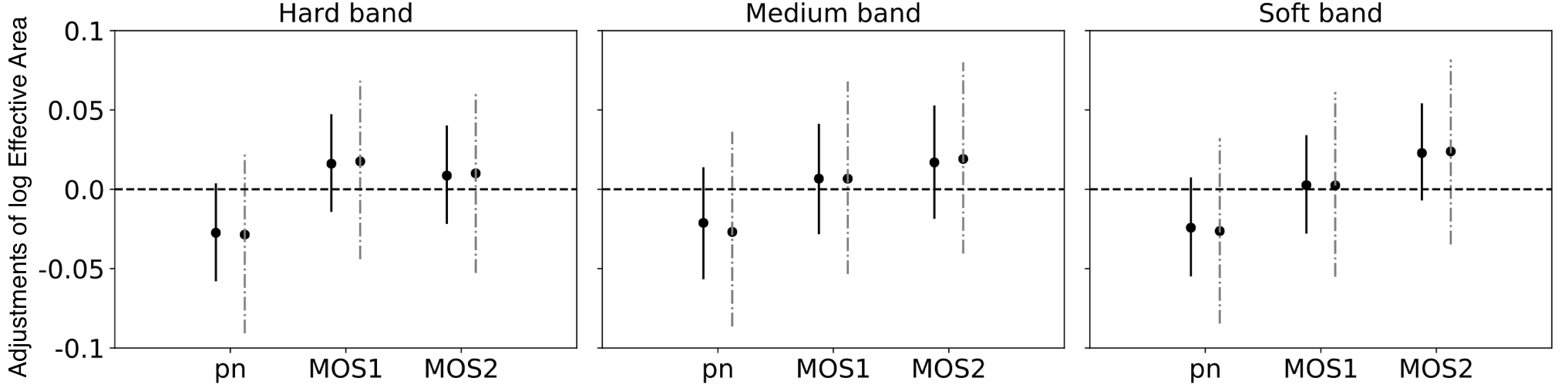
The log-Normal model is fit to the three datasets separately, with $\beta=0.014,0.083$ and $0.022$ respectively for the hard, median, and soft bands, but with $\alpha=1.5$ for all three. We again use $b_{i}=0$ and try $\tau_{i}=0.025$ and $\tau_{i}=0.05$. Figure 6 shows the resulting adjustments of the log-scale Effective Area, and confirms the astronomers’ expectation that no adjustment is needed for 2XMM, regardless of the choice of the $\tau_{i}$. In contrast to Table 5, Table 6 (also in Appendix A) shows a much more stable patterns of proportion of prior information for 2XMM data.

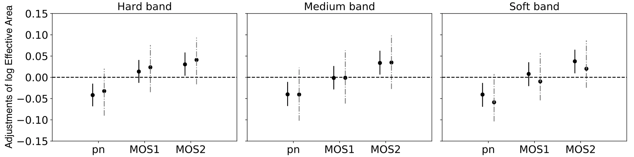
XCAL consists of bright AGN from the XMM-Newton cross-calibration sample²² 2 See Section 4 in http://xmm2.esac.esa.int/docs/documents/CAL-TN-0052.ps.gz. The image data are clipped, using a standard XMM software task (called epatplot), to eliminate the regions affected non-trivially by pileup. The amount of clipping depends on the observed source intensity: unused regions are larger for brighter sources (Marshall et al.,, 2018). The initial estimate of the Effective Area is then adjusted according to lookup tables (from other in-flight data) to account for the unused regions. Like the 2XMM data, XCAL data are composed of three datasets: the hard (94 sources), medium (103), and soft (108) bands, all measured by three instruments, pn, MOS1 and MOS2. We use the same procedure and hyperparameters as in Section 4.2, except we set $\beta=8.0\times 10^{-4},8.6\times 10^{-3}$ and $6.8\times 10^{-4}$ respectively for hard, median, and soft bands.

Figure 7 demonstrates that adjustment of the Effective Areas is needed to align the measured fluxes across the detectors. Results are presented for four sources from the medium band data, where the left three bars—corresponding to three instruments—depict the $95\%$ intervals (mean $\pm$ 2 given standard deviations) for the log-fluxes obtained by a standard astronomical method. The right two bars—corresponding to two choices of the prior variance $\tau_{i}$—represent the $95\%$ posterior intervals of log-fluxes after adjustment using our log-Normal model. This visualization illustrates the reliability of our calibration of Effective Areas, as it helps to bring together the varied flux estimates from individual detectors in a statistically principled way. In particular, we see that the posterior mean of the log-flux is rather robust to the choice of $\tau_{i}$, yet the corresponding posterior variance respects astronomers’ a priori knowledge as coded into $\tau_{i}$.

Finally, we show how to adjust the Effective Areas of each instrument to obtain the results illustrated in the rightmost interval in each panel of Figure 7. Figure 8 shows the necessary adjustment of $\bm{B}$ for hard band (left), medium band (middle) and soft band (right). For all these bands, we adjust the Effective Area of pn downward and that of MOS2 upward.

To check how well the log-Normal model captures the observed variability in the data, we use residual plots to visualize the goodness-of-fit. Figure 9 plots the standardized residuals $\widehat{\mathcal{R}}_{ij}$ for the data analyzed in Section 4.3 with $\tau_{i}=0.05$, with the left panels denoting residuals from the log-Normal model and the right panels from the log-$t$ model (see the two expressions of $\widehat{\mathcal{R}}_{ij}$ in (3.1)). Nearly all residuals fall in $[-3,\,3]$ under the log-Normal model and $[-2,\,2]$ under the log-$t$ model. The observations of 3C111 in all three energy bands are the only outliers under the log-Normal model but are not outliers under the log-$t$ model, confirming the latter’s ability to handle outliers. The adjusted Effective Areas and the estimated fluxes are not too sensitive to whether or not the outliers are excluded. Thus the log-Normal model is acceptable for the data in Section 4.3.

We also employ a posterior predictive check (Meng,, 1994; Gelman et al.,, 1996) for the log-Normal model. In a posterior predictive check, one chooses test statistics and computes the posterior predictive $p$-value. The test statistics we choose are

which reflect the relative magnitudes of the log scale Effective Areas. None of the posterior predictive $p$-values for any of our datasets are significant, i.e., we never fail the posterior predictive check. This does not, however, imply that no serious model defects exist. Below we discuss directions for improving our models and ultimately the reliability of the proposed concordance adjustments.

In Section 2, we adopt a Bayesian perspective, which leads to the log-Normal model. Alternatively, we could view $b_{i}$ as a noisy observation with known variance $\tau_{i}^{2}$: ${b}_{i}{\rm\stackrel{{\scriptstyle indep}}{{\sim}}}\mathcal{N}({B}_{i},\tau_{i}^{2})$. Together with (2.2), this gives a multivariate Normal regression model and can be fit via maximum likelihood estimation (MLE). In particular, when $\bm{\sigma^{2}}$ is known, Proposition 1 in Appendix E.1 gives closed-form expressions when all the instruments measure all sources, which implies the asymptotic properties of the MLEs (Corollary 1). Furthermore, the standardized residual sum of squares follows a $\chi^{2}$ distribution, which enables testing of the goodness-of-fit; see Appendix E.2 for details.

When the variances $\bm{\sigma^{2}}$ are unknown, in principle, we can still obtain the (asymptotic) variance of the MLEs by calculating the observed/expected Fisher information. However, the number of unknown parameters we consider, $2N+M$, grows with the number of observations $NM+N$. Conditions on the relationship between $N$ and $M$ that would ensure the classical asymptotic theory for MLEs would be of interest to those who prefer likelihood inference. Furthermore, under such conditions, these estimators should be approximately valid even if the Normal assumptions made in (2.2) for the $e_{ij}$ fail. In this case, the variance of the estimator requires a more complicated “sandwich” formula (Freedman,, 2006), involving both the Fisher information and the variance of the score function. We say approximately valid because the half-variance correction of Section 2 would depend on the log-Normal assumption. Consequently, when the variance is large, the half-variance correction can be misleading if the log-Normal assumption is severely violated.

As usual, the likelihood method is closely related to the Bayesian approach. For example, when $\bm{\sigma^{2}}$ is known, the MLEs of $\bm{B}$ and $\bm{G}$ correspond to the MAP estimates defined in (2.10), which also have the intuitive interpretation as shrinkage estimators. When the variances are unknown, the likelihood function is unbounded at the boundary of the parameter space ($\sigma_{i}^{2}=0$). The conjugate priors for variance parameters in the Bayesian model regularize the likelihood and give a proper posterior distribution. This is another reason we adopt the Bayesian approach.

References

- Appenzeller, (2012) Appenzeller, I. (2012). Introduction to astronomical spectroscopy, volume 9. Cambridge University Press.
- Bhaumik and Gibbons, (2005) Bhaumik, D. K. and Gibbons, R. D. (2005). Confidence regions for random-effects calibration curves with heteroscedastic errors. Technometrics, 47(2):223–231.
- Bilder and Loughin, (2014) Bilder, C. R. and Loughin, T. M. (2014). Analysis of categorical data with R. CRC Press.
- (4) Chandra X-ray Center (2017a). The Chandra proposers’ observatory guide, chapter 2. Accessed: 2018-02-28.
- (5) Chandra X-ray Center (2017b). The Chandra proposers’ observatory guide, chapter 3. Accessed: 2018-02-28.
- Chandra X ray observatory, (2009) Chandra X ray observatory (2009). E0102-72.3: Adding a new dimension to an old explosion. http://chandra.harvard.edu/photo/2009/e0102/.
- Drake et al., (2006) Drake, J. J., Ratzlaffa, P., Kashyapa, V., Edgara, R., Izemb, R., Jeriusa, D., Siemiginowskaa, A., and Vikhlinina, A. (2006). Monte Carlo processes for including Chandra instrument response uncertainties in parameter estimation studies. In SPIE Astronomical Telescopes + Instrumentation, pages 62701I–62701I. International Society for Optics and Photonics.
- Efron and Morris, (1975) Efron, B. and Morris, C. N. (1975). Data analysis using Stein’s estimator and its generalizations. Journal of the American Statistical Association, 70(350):311–319.
- Freedman, (2006) Freedman, D. A. (2006). On the so-called “Huber sandwich estimator” and “robust standard errors”. The American Statistician, 60(4):299–302.
- Gelman et al., (1996) Gelman, A., Meng, X.-L., and Stern, H. (1996). Posterior predictive assessment of model fitness via realized discrepancies. Statistica Sinica, 6(4):733–760.
- Geman and Geman, (1984) Geman, S. and Geman, D. (1984). Stochastic relaxation, Gibbs distributions, and the Bayesian restoration of images. IEEE Transactions on Pattern Analysis and Machine Intelligence, 6:721–741.
- George et al., (1992) George, I. M., Arnaud, K. A., Pence, B., and Ruamsuwan, L. (1992). Calibration sources for spectral analysis. Legacy, 2.
- Gibbons and Bhaumik, (2001) Gibbons, R. D. and Bhaumik, D. K. (2001). Weighted random-effects regression models with application to interlaboratory calibration. Technometrics, 43(2):192–198.
- Graessle et al., (2006) Graessle, D. E., Evans, I. N., Glotfelty, K., He, X. H., Evans, J. D., Rots, A. H., Fabbiano, G., and Brissenden, R. J. (2006). The Chandra X-ray observatory calibration database (CalDB): building, planning, and improving. Proc. SPIE, 6270:62701X–62701X–12.
- Guainazzi et al., (2015) Guainazzi, M., David, L., Grant, C. E., Miller, E., Natalucci, L., Nevalainen, J., Petre, R., and Audard, M. (2015). On the in-flight calibration plans of modern X-ray observatories. Journal of Astronomical Telescopes, Instruments, and Systems, 1(4):047001.
- Hannig et al., (2017) Hannig, J., Feng, Q., Iyer, H., Wang, C., and Liu, X. (2017). Fusion learning for inter-laboratory comparisons. Journal of Statistical Planning and Inference.
- Hastings, (1970) Hastings, W. (1970). Monte Carlo sampling methods using Markov chains and their applications. Biometrika, 57(1):97–109.
- Hoffman and Gelman, (2014) Hoffman, M. D. and Gelman, A. (2014). The No-U-Turn sampler: Adaptively setting path lengths in Hamiltonian Monte Carlo. Journal of Machine Learning Research, 15(1):1593–1623.
- IACHEC, (2017) IACHEC (2017). International Astronomical Consortium for High Energy Calibration. http://web.mit.edu/iachec/.
- Kashyap et al., (2008) Kashyap, V., Lee, H., Siemiginowska, A., McDowell, J., Rots, A., Drake, J., Ratzlaff, P., Zezas, A., Izem, R., Connors, A., and van Dyk, D. (2008). How to handle calibration uncertainties in high-energy astrophysics. Proceedings of SPIE (Observatory Operation: Strategies, Processes, and System II), 7016:23 (8pp).
- Lange et al., (1989) Lange, K. L., Little, R. J., and Taylor, J. M. (1989). Robust statistical modeling using the t distribution. Journal of the American Statistical Association, 84(408):881–896.
- Lee et al., (2011) Lee, H., Kashyap, V. L., Van Dyk, D. A., Connors, A., Drake, J. J., Izem, R., Meng, X.-L., Min, S., Park, T., Ratzlaff, P., and Siemiginowska, A. (2011). Accounting for calibration uncertainties in X-ray analysis: effective areas in spectral fitting. The Astrophysical Journal, 731(2):126 (19pp).
- Madsen et al., (2016) Madsen, K. K., Beardmore, A. P., Forster, K., Guainazzi, M., Marshall, H. L., Miller, E. D., Page, K. L., and Stuhlinger, M. (2016). IACHEC cross-calibration of Chandra, Nustar, Swift, Suzaku, XMM-Newton with 3C 273 ANDPKS 2155-304. The Astronomical Journal, 153(1):2(17pp).
- Marshall et al., (2018) Marshall, H., Kashyap, V., Chen, Y., Meng, X.-L., and Wang, X. (2018). Concordance: In-flight calibration of X-ray telescopes without absolute references. In Preparation.
- Matthews and Havey, (2010) Matthews, G. and Havey, Jr., K. (2010). Ten years of Chandra: reflecting back on engineering lessons learned during the design, fabrication, integration, test, and verification of NASA’s great X-ray observatory. Proc. SPIE, 7738:77380Y–77380Y–13.
- Meng, (1994) Meng, X.-L. (1994). Posterior predictive p-values. The Annals of Statistics, 22(3):1142–1160.
- Meng, (2018) Meng, X.-L. (2018). Conducting highly-principled data science: A statistician’s job and joy. Statistics and Probability Letters. To appear.
- Metropolis et al., (1953) Metropolis, N., Rosenbluth, A., Rosenbluth, M., Teller, A., and Teller, E. (1953). Equations of state calculations by fast computing machines. Journal of Chemical Physics, 21(6):1087–1092.
- Morris, (1983) Morris, C. N. (1983). Parametric empirical Bayes inference: theory and applications. Journal of the American Statistical Association, 78(381):47–55.
- Neal, (2011) Neal, R. M. (2011). MCMC using Hamiltonian dynamics. In Brooks, S., Gelman, A., Jones, G., and Meng, X.-L., editors, Handbook of Markov chain Monte Carlo, volume 2. CRC Press.
- Nevalainen et al., (2010) Nevalainen, J., David, L., and Guainazzi, M. (2010). Cross-calibrating X-ray detectors with clusters of galaxies: An IACHEC study. Astronomy & Astrophysics, 523:A22.
- Plucinsky et al., (2017) Plucinsky, P. P., Beardmore, A. P., Foster, A., Haberl, F., Miller, E. D., Pollock, A. M., and Sembay, S. (2017). SNR 1E 0102.2-7219 as an X-ray calibration standard in the 0.5-1.0 keV bandpass and its application to the CCD instruments aboard Chandra, Suzaku, Swift and XMM-Newton. Astronomy & Astrophysics, 597(A35).
- Read et al., (2014) Read, A. M., Guainazzi, M., and Sembay, S. (2014). Cross-calibration of the XMM-Newton EPIC pn and MOS on-axis effective areas using 2XMM sources. Astronomy & Astrophysics, 564:A75.
- Rubin, (1976) Rubin, D. B. (1976). Inference and missing data. Biometrika, 63(3):581–592.
- Schellenberger et al., (2015) Schellenberger, G., Reiprich, T., Lovisari, L., Nevalainen, J., and David, L. (2015). XMM-Newton and Chandra cross-calibration using HIFLUGCS galaxy clusters-systematic temperature differences and cosmological impact. Astronomy & Astrophysics, 575:A30.
- Schwartz, (2014) Schwartz, D. A. (2014). Invited review article: The Chandra X-ray observatory. Review of Scientific Instruments, 85(6):061101.
- Sembay et al., (2010) Sembay, S., Guainazzi, M., Plucinsky, P., and Nevalainen, J. (2010). Defining high-energy calibration standards: IACHEC (International Astronomical Consortium for High-Energy Calibration). In AIP Conf. Proceedings, volume 1248, pages 593–594. AIP.
- Seward, (1992) Seward, F. (1992). Calibration sources for spectral analysis.
- Stan Development Team, (2015) Stan Development Team (2015). Stan Modeling Language User’s Guide and Reference Manual, Version 2.10.0.
- Stan Development Team, (2016) Stan Development Team (2016). Pystan: the Python interface to Stan.
- Tanner and Wong, (1987) Tanner, M. A. and Wong, W. H. (1987). The calculation of posterior distributions by data augmentation. Journal of the American Statistical Association, 82(398):528–540.
- Tsujimoto et al., (2011) Tsujimoto, M., Guainazzi, M., Plucinsky, P. P., Beardmore, A. P., Ishida, M., Natalucci, L., Posson-Brown, J. L., Read, A. M., Saxton, R. D., and Shaposhnikov, N. V. (2011). Cross-calibration of the X-ray instruments onboard the Chandra, Integral, RXTE, Suzaku, Swift, and XMM-Newton observatories using G21. 5–0.9. Astronomy & Astrophysics, 525:A25.
- Watson et al., (2009) Watson, M. G., Schröder, A. C., Fyfe, D., Page, C. G., Lamer, G., Mateos, S., Pye, J., Sakano, M., Rosen, S., Ballet, J., Barcons, X., Barret, D., Boller, T., Brunner, H., Brusa, M., Caccianiga, A., Carrera, F. J., Ceballos, M., Della Ceca, R., Denby, M., Denkinson, G., Dupuy, S., Farrell, S., Fraschetti, F., Freyberg, M. J., Guillout, P., Hambaryan, V., Maccacaro, T., Mathiesen, B., McMahon, R., Michel, L., Motch, C., Osborne, J. P., Page, M., Pakull, M. W., Pietsch, W., Saxton, R., Schwope, A., Severgnini, P., Simpson, M., Sironi, G., Stewart, G., Stewart, I. M., Stobbart, A.-M., Tedds, J., Warwick, R., Webb, N., West, R., Worrall, D., and Yuan, W. (2009). The XMM-Newton serendipitous survey. V. The Second XMM-Newton serendipitous source catalogue. Astronomy and Astrophysics, 493:339–373.
- Weatherhead et al., (1998) Weatherhead, E. C., Reinsel, G. C., Tiao, G. C., Meng, X.-L., Choi, D., Cheang, W.-K., Keller, T., DeLuisi, J., Wuebbles, D. J., Kerr, J. B., and Miller, A. (1998). Factors affecting the detection of trends: Statistical considerations and applications to environmental data. Journal of Geophysical Research: Atmospheres, 103(D14):17149–17161.
- XMM Catalogue public pages, (2008) XMM Catalogue public pages (2008). XMM-Newton serendipitous source catalogue: 2XMM. http://xmmssc-www.star.le.ac.uk/Catalogue/xcat_public_2XMM.html.
- Xu et al., (2014) Xu, J., Van Dyk, D. A., Kashyap, V. L., Siemiginowska, A., Connors, A., Drake, J., Meng, X.-L., Ratzlaff, P., and Yu, Y. (2014). A fully Bayesian method for jointly fitting instrumental calibration and X-ray spectral models. The Astrophysical Journal, 794(2):97.
Appendix A Tables of Data Description and Prior Influence