Outage Analysis of Ambient Backscatter Communication Systems

Wenjing Zhao Gongpu Wang Saman Atapattu Chintha Tellambura Hao Guan ^†^†thanks: W. Zhao and G. Wang are with School of Computer and Information Technology, Beijing Jiaotong University, Beijing 100044, China (e-mail: wenjing_bjtu@163.com; gpwang@bjtu.edu.cn).^†^†thanks: S. Atapattu are with the Department of Electrical and Electronic Engineering, The University of Melbourne, Melbourne, VIC 3010, Australia (e-mail: saman.atapattu@unimelb.edu.au).^†^†thanks: C. Tellambura is with the Department of Electrical and Computer Engineering, University of Alberta, Edmonton, AB T6G 2V4, Canada (e-mail: chintha@ ece.ualberta.ca).^†^†thanks: H. Guan is with Nokia Bell Labs, Beijing, China (e-mail:hao.guan@nokia-sbell.com).

Abstract

This paper addresses the problem of outage characterization of an ambient backscatter communication system with a pair of passive tag and reader. In particular, an exact expression for the effective channel distribution is derived. Then, the outage probability at the reader is analyzed rigorously. Since the expression contains an infinite sum, a tight truncation error bound has been derived to facilitate precise numerical evaluations. Furthermore, an asymptotic expression is provided for high signal-to-noise ratio (SNR) regime.

Index Terms:

Ambient backscatter, Internet of Things (IoT), outage probability, performance analysis.

I Introduction

Backscatter communication systems, such as Radio Frequency Identification (RFID) system, enable connecting massive small computing devices specially for applications in Internet of Things (IoT) [1]. The traditional RFID system typically consists of a tag and a reader. The reader first generates and transmits an electromagnetic wave signal to the tag, and then the tag receives and backscatters the signal to the reader.

One disadvantage for the RFID system is that the reader needs an oscillator to transmit a carrier signal, for which dedicated encoding/decoding circuitry and power supply are required [2]. While these are essential components for a successful communication, such in-built technology may no longer be promising for small-scale devices. To overcome such overheads, ambient backscatter prototypes are proposed in [3, 4].

The ambient backscatter technology utilizes environmental wireless signals (e.g., digital TV broadcasting, cellular or Wi-Fi) for both energy harvesting and information transmission, which avoids battery as well as manual maintenance. Specifically, the tag indicates bit 1 or bit 0 through reflecting or non-reflecting state, and the reader decodes the received backscattered signal accordingly [5]. Ambient backscatter may be widely used for future applications (e.g., many applications in IoT with sensors located in dangerous spots filled with poisonous gases/liquids, or inside building walls) that are inconvenient and unsafe for wired communications [6].

The performance analysis of the ambient backscatter communication is considered over real Gaussian channels in [7], and complex Gaussian channels in [8, 9]. The bit error rate (BER) is derived and the BER-based outage probability is obtained in [7] for ambient bakcscatter communication systems with energy detector. In addition, the outage capacity optimization problem is investigated in [8] when successive interference cancellation (SIC) method is applied. Besides, the BER-based outage probability of a semi-coherent detection scheme is calculated in [9] in the case of perfect and imperfect channel state information (CSI), respectively.

To our best knowledge, effective channel distribution for ambient backscatter communication systems has not be addressed and the outage performance based on signal-to-noise ratio (SNR) remains an open problem, which is the focus of this paper.

In this paper, we consider an ambient backscatter communication system over real Gaussian channels. We derive an exact expression for the effective channel distribution in this system. Particularly, we evaluate the outage performance and analyse its asymptotic outage performance at high transmit SNR. Moreover, since the derived outage probability is the summation of infinite items, the corresponding truncation error bound is calculated.

II System Model

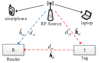
Refer to caption — Fig. 1: An ambient backscatter communication system.

We consider an ambient backscatter communication system comprised of an ambient RF source ( $S$ ) and a pair of passive tag ( $T$ ) and reader ( $R$ ) (Fig. 1). While the RF source communicates with its legacy users (e.g., smartphones, laptops, etc.), both tag and reader may also receive that source signal. The tag first harvests energy from the source signal, and then communicates with the reader via ambient backscatter. Particularly, the tag can backscatter or consume the energy of the received signal to represent two states “1” or “0” for the reader, respectively [5].

The fading channels of $S-R$ , $S-T$ , and $T-R$ links are denoted as $\tilde{h}_{sr}$ , $\tilde{h}_{st}$ and $\tilde{h}_{tr}$ , respectively, which are real Gaussian random variables (RVs) distributed as $\tilde{h}_{sr}\sim\mathcal{N}(0,\tilde{\sigma}_{sr}^{2})$ , $\tilde{h}_{st}\sim\mathcal{N}(0,\tilde{\sigma}_{st}^{2})$ and $\tilde{h}_{tr}\sim\mathcal{N}(0,\tilde{\sigma}_{tr}^{2})$ , where $\tilde{\sigma}_{sr}^{2}$ , $\tilde{\sigma}_{st}^{2}$ and $\tilde{\sigma}_{tr}^{2}$ are channel variances. Further, the corresponding distances are $d_{sr}$ , $d_{st}$ and $d_{tr}$ , respectively. Without loss of generality, we consider time instance $n$ . The signal received at the tag can be given as

y_{t}(n)=\frac{\tilde{h}_{st}}{\sqrt{d_{st}^{\alpha}}}s(n),

(1)

where $s(n)$ is the source signal with the average power $P$ , and $\alpha$ is the path-loss exponent. The signal backscattered by the tag can be written as

x(n)=\eta B(n)y_{t}(n),

(2)

where $B(n)\in\{0,1\}$ is a binary symbol and $\eta\in[0,1]$ is the attenuation factor. Then, the received signal at the reader can be given as [5]

\begin{split}y_{r}(n)&=\frac{\tilde{h}_{sr}}{\sqrt{d_{sr}^{\alpha}}}s(n)+\frac{\tilde{h}_{tr}}{\sqrt{d_{tr}^{\alpha}}}x(n)+w(n)\\ &=hs(n)+w(n),\end{split}

(3)

where $w(n)$ is the additive white Gaussian noise (AWGN) at the reader with zero mean and $\sigma_{w}^{2}$ variance, and $h$ is the effective channel gain which can be given for two states as

\displaystyle h

\displaystyle=\left\{\begin{array}[]{ll}h_{sr},&B(n)=0,\\ h_{sr}+\eta h_{st}h_{tr},&B(n)=1,\end{array}\right.

where $h_{sr}\triangleq\frac{\tilde{h}_{sr}}{\sqrt{d_{sr}^{\alpha}}}\sim\mathcal{N}(0,\sigma_{sr}^{2})$ , $h_{st}\triangleq\frac{\tilde{h}_{st}}{\sqrt{d_{st}^{\alpha}}}\sim\mathcal{N}(0,\sigma_{st}^{2})$ , and $h_{tr}\triangleq\frac{\tilde{h}_{tr}}{\sqrt{d_{tr}^{\alpha}}}\sim\mathcal{N}(0,\sigma_{tr}^{2})$ with $\sigma_{sr}^{2}=\frac{\tilde{\sigma}_{sr}^{2}}{d_{sr}^{\alpha}}$ , $\sigma_{st}^{2}=\frac{\tilde{\sigma}_{st}^{2}}{d_{st}^{\alpha}}$ and $\sigma_{tr}^{2}=\frac{\tilde{\sigma}_{tr}^{2}}{d_{tr}^{\alpha}}$ .

III Performance Analysis

III-A Effective Channel and SNR Distributions

We first derive the probability density function (PDF) of the effective channel, $f_{h}(x)$ , which can be given as

\displaystyle f_{h}(x)=\left\{\begin{array}[]{ll}\frac{1}{\sqrt{2\pi\sigma^{2}_{sr}}}e^{-\frac{x^{2}}{2\sigma^{2}_{sr}}},\hskip 55.48277ptB(n)=0,&\\ \frac{e^{\frac{\sigma^{2}_{sr}}{4\eta^{2}\sigma^{2}_{st}\sigma^{2}_{tr}}}}{\sqrt{2\pi^{3}\sigma^{2}_{sr}}}e^{-\frac{x^{2}}{2\sigma_{sr}^{2}}}\displaystyle\sum_{k=0}^{\infty}\frac{2^{k}\Gamma^{2}\left(k+\frac{1}{2}\right)x^{2k}}{(2k)!\sigma_{sr}^{2k}}&\\ \hskip 8.5359pt\times W_{-k,0}\left(\frac{\sigma^{2}_{sr}}{2\eta^{2}\sigma^{2}_{st}\sigma^{2}_{tr}}\right),\hskip 18.49411ptB(n)=1,&\end{array}\right.

where $W_{a,b}(\cdot)$ and $\Gamma(\cdot)$ are the Whittaker function [10, eq. (9.223)] and the Gamma function [10, eq. (8.310.1)], respectively. The proof is in Appendix -A.

The receive SNR at the reader is $\rho=\frac{Ph^{2}}{\sigma^{2}_{w}}=\bar{\rho}h^{2}$ where $\bar{\rho}=\frac{P}{\sigma^{2}_{w}}$ may be the average transmit SNR. With a variable transformation for (III-A), we can derive the PDF of $\rho$ , $f_{\rho}(x)$ , as

\begin{split}f_{\rho}(x)&=\frac{\left[f_{h}\left(\sqrt{\frac{x}{\bar{\rho}}}\right)+f_{h}\left(-\sqrt{\frac{x}{\bar{\rho}}}\right)\right]}{2\sqrt{\bar{\rho}x}}=\frac{f_{h}\left(\sqrt{\frac{x}{\bar{\rho}}}\right)}{\sqrt{\bar{\rho}x}},\end{split}

(9)

where the second equality follows as the PDF $f_{h}(x)$ is an even function, i.e., $f_{h}(x)=f_{h}(-x)$ .

III-B Outage Probability

The outage probability is the probability that the SNR at the reader falls below a certain predetermined threshold $\rho_{t}$ . Thus, it can be derived as

	$\displaystyle P_{o}$	$\displaystyle=\Pr[\rho\leq\rho_{t}]=\int_{0}^{\rho_{t}}f_{\rho}(x)dx$
		$\displaystyle=\left\{\begin{array}[]{ll}\textrm{erf}\left(\sqrt{\frac{\rho_{t}}{2\bar{\rho}\sigma^{2}_{sr}}}\right),&\hskip-34.14322ptB(n)=0,\\ \displaystyle\sum_{k=0}^{\infty}\frac{2^{2k}\Gamma^{2}(k+\frac{1}{2})}{\sqrt{\pi^{3}}(2k)!}W_{-k,0}\left(\frac{\sigma_{sr}^{2}}{2\eta^{2}\sigma_{st}^{2}\sigma_{tr}^{2}}\right)\\ \hskip-1.42271pt\times e^{\frac{\sigma_{sr}^{2}}{4\eta^{2}\sigma_{st}^{2}\sigma_{tr}^{2}}}\gamma\left(k+\frac{1}{2},\frac{\rho_{t}}{2\bar{\rho}\sigma^{2}_{sr}}\right),&\hskip-34.14322ptB(n)=1,\end{array}\right.$

where $\textrm{erf}(\cdot)$ and $\gamma(\cdot,\cdot)$ are the error function [10, eq. (8.250.1)] and the incomplete gamma function [10, eq. (8.350.1)], respectively. The equation (III-B) can be obtained by following from [10, eq. (3.321.2)], [10, eq. (8.250.1)] and [10, eq. (3.381.1)].

III-C Truncation Error Bound

Since the outage probability expression for $B(n)=1$ case in (III-B) is with an infinite sum, it is a challenge for numerical calculation. We therefore truncate it into a finite number of terms $T$ in order to ensure a given numerical accuracy requirement. Then, we bound the truncation error as

\begin{split}|\epsilon_{T}|&\leq\frac{\Psi\left(\frac{1}{2},0,\nu\right)}{\sqrt{\pi\nu}T!}\biggr[\sqrt{\frac{2\rho_{t}}{\sigma^{2}_{sr}\bar{\rho}}}\gamma\left(T+1,\frac{\rho_{t}}{2\sigma^{2}_{sr}\bar{\rho}}\right)\\ &\,\,\,\,\,\,\,\,\,\,\,\,\,\,\,\,\,\,\,\,\,\,\,\,\,\,\,\,\,\,\,\,\,\,\,\,\,\,\,~~~~~~~-2\gamma\left(T+\frac{3}{2},\frac{\rho_{t}}{2\sigma^{2}_{sr}\bar{\rho}}\right)\biggr],\end{split}

(13)

where $\nu=\frac{\sigma_{sr}^{2}}{2\eta^{2}\sigma_{st}^{2}\sigma_{tr}^{2}}$ , and $\Psi(\cdot,\cdot,\cdot)$ is the confluent hypergeometric function [10, eq. (9.211.4)]. The proof is in Appendix -B.

III-D Asymptotic Analysis for High SNR

To further investigate the ambient backscatter system, we approximate outage of the reader for large SNR as

\displaystyle P_{o}\approx\left\{\begin{array}[]{ll}\sqrt{\frac{2\rho_{t}}{\pi\sigma_{sr}^{2}}}\frac{1}{\sqrt{\bar{\rho}}},&\hskip-8.5359ptB(n)=0,\\ \frac{\sqrt{2\rho_{t}}e^{\frac{\sigma_{sr}^{2}}{4\eta^{2}\sigma_{st}^{2}\sigma_{tr}^{2}}}W_{0,0}\left(\frac{\sigma_{sr}^{2}}{2\eta^{2}\sigma_{st}^{2}\sigma_{tr}^{2}}\right)}{\sqrt{\pi\sigma_{sr}^{2}}}\frac{1}{\sqrt{\bar{\rho}}},&\hskip-8.5359ptB(n)=1.\end{array}\right.

The proof is in Appendix -C.

Interestingly, when transmit SNR tends to infinity, we get that the diversity gain is $-\underset{\textrm{SNR}\rightarrow\infty}{\lim}\frac{\log P_{\textrm{out}}}{\log\textrm{SNR}}=\frac{1}{2}$ for both cases $B(n)=0$ and $B(n)=1$ . Accordingly, when power is big enough, the outage probability of the reader is inversely proportional to square root of the power.

IV Numerical and Simulation Results

This section provides simulation results based on the system model in Section II and numerical results based on the analytical results in Section III. Here, the attenuation factor $\eta$ is set as 0.7. Besides, we assume $\sigma_{sr}^{2}=\sigma_{st}^{2}=1$ and $\sigma_{tr}^{2}=3$ , unless otherwise specified.

For the state $B(n)=1$ , we derive a truncation error bound (13). Fig. 2 shows the relative error versus the number of terms $T$ when $\bar{\rho}=3$ dB for $\rho_{t}=-3$ dB and $\rho_{t}=7$ dB. We calculate the relative error with truncation as $\frac{|\textrm{exact}-\textrm{truncated}|}{\textrm{exact}}$ ; the relative error with bound as $\frac{\textrm{error bound in}\,\eqref{e_errbound}}{\textrm{exact value}}$ ; the exact value with numerical integration; and the truncated value for different $T$ by using (III-B). The relative error with truncation is less than $10^{-5}$ when $T>2$ and $T>5$ for $\rho_{t}=-3$ dB and $\rho_{t}=7$ dB, respectively. The relative error with bound is less than $10^{-5}$ when $T>3$ and $T>8$ for $\rho_{t}=-3$ dB and $\rho_{t}=7$ dB, respectively. This shows the tightness of the bound. Moreover, by observation, we may say that a very accurate value can be calculated using small $T$ .

Fig. 3 illustrates the outage probability $P_{o}$ versus the average transmit SNR $\bar{\rho}$ when $\rho_{t}=2$ dB and $\rho_{t}=15$ dB. The outage probability decreases with the increasing average transmit SNR. The asymptotic expressions (III-D) also approach the exact values asymptotically at high SNR. Since the diversity gain is 1/2, the slope of the asymptotic outage curves is 1/2.

Fig. 4 depicts the outage probabilities $P_{o}$ versus the distance $d_{tr}$ between the tag and the reader. We consider both cases of SNR $\bar{\rho}=10$ dB and $\bar{\rho}=20$ dB, respectively. We set $\rho_{t}=2\,$ dB, $\alpha=3$ , $d_{sr}=20$ meters and $d_{st}=20$ meters. Besides, the channel variances $\tilde{\sigma}_{sr}^{2}$ , $\tilde{\sigma}_{st}^{2}$ and $\tilde{\sigma}_{tr}^{2}$ are set as 1, 1 and 3, respectively. The outage probability $P_{o}$ is a constant in the case of $B(n)=0$ due to no transmission between the tag and the reader. However, when enlarging the distance $d_{tr}$ between the tag and the reader, the outage probability $P_{o}$ witnesses a upward trend in the case of $B(n)=1$ . For example, if we expect $P_{o}<10^{-4}$ , the distance $d_{tr}$ between the tag and the reader should not exceed 3 meters when $\bar{\rho}=10$ dB and 7 meters when $\bar{\rho}=20$ dB.

V Conclusion

Ambient backscatter, a new form of wireless communication, has potential commercial value as well as a series of open problems. In this paper, we first derived the effective channel distribution for the ambient backscatter communication system. We next analyzed the outage probabilities, its truncation error bound as well as the asymptotic outage probabilities at high SNR. It was found that the asymptotic outage probabilities could well approach the exact values, and our truncation error bound could provide a reasonable estimation of the truncation terms.

-A Proof of (III-A)

The distribution of any real Gaussian channel $h_{ab}\in\{h_{sr},h_{st},h_{rt}\}$ is

\displaystyle f_{h_{ab}}(x)=\frac{1}{\sqrt{2\pi\sigma^{2}_{ab}}}e^{-\frac{x^{2}}{2\sigma^{2}_{ab}}},

(16)

where $\sigma^{2}_{ab}\in\{\sigma^{2}_{sr},\sigma^{2}_{st},\sigma^{2}_{rt}\}$ .

In the case of $B(n)=1$ , we have $h=h_{sr}+\eta h_{st}h_{tr}$ . The distribution $f_{\xi}(x)$ of $\xi=\eta h_{st}h_{tr}$ can be shown as [11]

f_{\xi}(x)=\frac{1}{\pi\eta\sqrt{\sigma^{2}_{st}\sigma^{2}_{tr}}}K_{0}\left(\frac{|x|}{\eta\sqrt{\sigma^{2}_{st}\sigma^{2}_{tr}}}\right),

(17)

where $K_{\alpha}(\cdot)$ is the modified Bessel function of the second kind [10].

Since the two random variables $h_{sr}$ and $\xi$ are independent, the distribution $f_{h}(x)$ is the convolution of $f_{h_{sr}}(x)$ and $f_{\xi}(x)$ . Therefore, we can obtain

$\displaystyle f_{h}(x)$	$\displaystyle=\int_{-\infty}^{\infty}f_{h_{sr}}(x-z)f_{\xi}(z)\,dz$
	$\displaystyle\overset{\text{(a)}}{=}\frac{e^{-\frac{x^{2}}{2\sigma_{sr}^{2}}}}{\delta\varphi}\int_{0}^{\infty}K_{0}(\frac{z}{\varphi})e^{-\frac{z^{2}}{2\sigma_{sr}^{2}}}\left(e^{\frac{xz}{\sigma_{sr}^{2}}}+e^{-\frac{xz}{\sigma_{sr}^{2}}}\right)dz$
	$\displaystyle\overset{\text{(b)}}{=}\frac{2e^{-\frac{x^{2}}{2\sigma_{sr}^{2}}}}{\delta\varphi}\int_{0}^{\infty}K_{0}(\frac{z}{\varphi})e^{-\frac{z^{2}}{2\sigma_{sr}^{2}}}\cosh(\frac{xz}{\sigma_{sr}^{2}})dz$
	$\displaystyle\overset{\text{(c)}}{=}\frac{2e^{-\frac{x^{2}}{2\sigma_{sr}^{2}}}}{\delta\varphi}\sum_{k=0}^{\infty}\frac{x^{2k}}{\sigma_{sr}^{4k}(2k)!}\int_{0}^{\infty}K_{0}(\frac{z}{\varphi})e^{-\frac{z^{2}}{2\sigma_{sr}^{2}}}z^{2k}dz$
	$\displaystyle\overset{\text{(d)}}{=}\frac{e^{\frac{\nu}{2}}}{\delta}\sum_{k=0}^{\infty}\frac{2^{k}\Gamma^{2}(k+\frac{1}{2})W_{-k,0}(\nu)}{(2k)!\sigma_{sr}^{2k}}e^{-\frac{x^{2}}{2\sigma_{sr}^{2}}}x^{2k},$	(18)

where

\displaystyle\delta=\sqrt{2\pi^{3}\sigma^{2}_{sr}},\quad\varphi=\eta\sqrt{\sigma^{2}_{st}\sigma^{2}_{tr}},\quad\nu=\frac{\sigma_{sr}^{2}}{2\eta^{2}\sigma_{st}^{2}\sigma_{tr}^{2}},

(19)

(a) follows by two integrals having identical bounds, (b) follows by using the definition of hyperbolic cosine $\cosh x=\frac{1}{2}(e^{x}+e^{-x})$ , (c) follows by replacing $\cosh x$ with its series expression $\sum_{k=0}^{\infty}\frac{x^{2k}}{(2k)!}$ , and (d) follows from [10, eq. (6.631.3)].

-B Proof of (13)

On the basis of (III-B), the truncation error $\epsilon(T)$ with the number of terms $T$ can be bounded as

		$\displaystyle\epsilon(T)$
	$\displaystyle=$	$\displaystyle\frac{e^{\frac{\nu}{2}}}{\sqrt{\pi}\pi}\sum_{k=T+1}^{\infty}\frac{2^{2k}\Gamma^{2}\left(k+\frac{1}{2}\right)W_{-k,0}(\nu)}{(2k)!}\gamma\left(k+\frac{1}{2},\frac{\rho_{t}}{2\sigma^{2}_{sr}\bar{\rho}}\right)$
	$\displaystyle\overset{\text{(a)}}{=}$	$\displaystyle\frac{\sqrt{\nu}}{\pi}\sum_{k=T+1}^{\infty}\frac{1}{k!}\int_{0}^{\infty}\frac{e^{-\nu x}x^{k+\frac{1}{2}}}{(1+x)^{k+\frac{1}{2}}}dx\int_{0}^{\frac{\rho_{t}}{2\sigma^{2}_{sr}\bar{\rho}}}e^{-y}y^{k-\frac{1}{2}}dy$
	$\displaystyle\overset{\text{(b)}}{=}$	$\displaystyle\frac{\sqrt{\nu}}{\pi(T+1)!}\int_{0}^{\infty}\int_{0}^{\frac{\rho_{t}}{2\sigma^{2}_{sr}\bar{\rho}}}\frac{e^{-\nu x}x^{T+\frac{3}{2}}}{(1+x)^{T+\frac{3}{2}}}e^{-y}y^{T+\frac{1}{2}}$
		$\displaystyle~~~~~~~~~~~~~~~~~~~~~~~~~~~\times{{}_{1}F_{1}}\left(1;T+2;\frac{xy}{x+1}\right)dydx$
	$\displaystyle\overset{\text{(c)}}{=}$	$\displaystyle\frac{\sqrt{\nu}}{\pi T!}\int_{0}^{\infty}\int_{0}^{\frac{\rho_{t}}{2\sigma^{2}_{sr}\bar{\rho}}}\frac{e^{-\nu x}x^{\frac{1}{2}}}{(1+x)^{\frac{1}{2}}}e^{-y}y^{-\frac{1}{2}}$
		$\displaystyle~~~~~~~~~~~~~~~~~~~~~~~~~~~\times e^{\frac{xy}{x+1}}\gamma\left(T+1,\frac{xy}{x+1}\right)dydx$

	$\displaystyle\mathop{<}\limits^{(d)}$	$\displaystyle\frac{\sqrt{\nu}}{\pi T!}\int_{0}^{\infty}\frac{e^{-\nu x}x^{\frac{1}{2}}}{(1+x)^{\frac{1}{2}}}dx\int_{0}^{\frac{\rho_{t}}{2\sigma^{2}_{sr}\bar{\rho}}}\frac{\gamma(T+1,y)}{\sqrt{y}}dy$
	$\displaystyle=$	$\displaystyle\frac{\Psi(\frac{1}{2},0,\nu)}{\sqrt{\pi\nu}T!}\biggr[\sqrt{\frac{2\rho_{t}}{\sigma^{2}_{sr}\bar{\rho}}}\gamma\left(T+1,\frac{\rho_{t}}{2\sigma^{2}_{sr}\bar{\rho}}\right)$
		$\displaystyle\,\,\,\,\,\,\,\,\,\,\,\,\,\,\,\,\,\,\,\,\,\,\,\,\,\,\,\,\,\,\,\,\,\,\,\,\,\,\,~~~~~~~-2\gamma\left(T+\frac{3}{2},\frac{\rho_{t}}{2\sigma^{2}_{sr}\bar{\rho}}\right)\biggr],$

where $\nu$ is defined in (19), (a) is obtained from [10, eq. (9.222.1)] and [10, eq. (8.350.1)], (b) follows by setting $j=k-T-1$ and leveraging the integral representation of Hypergeometric function [10, eq. (9.211.4)], (c) utilizes the following equation

	${}_{1}F_{1}\left(1;T+2;\frac{xy}{x+1}\right)=(T+1)\left(\frac{xy}{x+1}\right)^{-(T+1)}e^{\frac{xy}{x+1}}$
	$\displaystyle\times\gamma\left(T+1,\frac{xy}{x+1}\right),$

(d) is based on $\frac{x}{x+1}<1$ for $x>0$ , and $\Psi(\cdot,\cdot,\cdot)$ is the confluent hypergeometric function [10, eq. (9.211.4)].

-C Proof of (III-D)

In the case of $B(n)=0$ and using series representation of the error function $\textrm{erf}(\cdot)$ [10, eq. (8.253.1)], we can expand (III-B) as

\displaystyle\textrm{erf}\left(\sqrt{\frac{\rho_{t}}{2\bar{\rho}\sigma^{2}_{sr}}}\right)=\frac{2}{\sqrt{\pi}}\displaystyle\sum_{k=0}^{\infty}\frac{(-1)^{k}{\rho_{t}}^{k+1/2}}{k!(2k+1)(2\bar{\rho}\sigma^{2}_{sr})^{k+1/2}}.

For $\bar{\rho}\rightarrow\infty$ , we consider the lowest exponent for $1/\bar{\rho}$ , i.e., the index $k=0$ . Similarly, in the case of $B(n)=1$ , we can expand $\gamma\left(\cdot,\cdot\right)$ in (III-B) as

\displaystyle\gamma\left(a,x\right)=\sum_{j=0}^{\infty}\frac{(-1)^{j}x^{a+j}}{j!(a+j)}.

We then consider the lowest exponent for $1/\bar{\rho}$ , i.e., the indies $k=0$ and $j=0$ . Thereby, when average transmit SNR tends to infinity, namely, $\bar{\rho}\rightarrow\infty$ , the asymptotic outage probability can be simplified as (III-D).

References

[1] A. Al-Fuqaha, M. Guizani, M. Mohammadi, M. Aledhari, and M. Ayyash, “Internet of things: A survey on enabling technologies, protocols, and applications,” IEEE Commun. Surveys Tuts., vol. 17, pp. 2347–2376, Jun. 2015.
[2] T. H. Lee, The design of CMOS Radio-Frequency integrated circuits. Cambridge Univ. Press, 1998.
[3] V. Liu, A. Parks, V. Talla, S. Gollakota, D. Wetherall, and J. R. Smith, “Ambient backscatter: wireless communication out of thin air,” in Proc. ACM SIGCOMM, Aug. 2013, pp. 39–50.
[4] A. N. Parks, A. Liu, S. Gollakota, and J. R. Smith, “Turbocharging ambient backscatter communication,” in Proc. ACM SIGCOMM, Aug. 2014, pp. 619–630.
[5] G. Wang, F. Gao, R. Fan, and C. Tellambura, “Ambient backscatter communication systems: Detection and performance analysis,” IEEE Trans. Commun., vol. 64, pp. 4836–4846, Nov. 2016.
[6] D. Kuester and Z. Popovic, “How good is your tag?: RFID backscatter metrics and measurements,” IEEE Microwave Mag., vol. 14, pp. 47–55, Jul. 2013.
[7] Y. Zhang, J. Qian, F. Gao, and G. Wang, “Ambient backscatter system with real source,” in IEEE Workshop on Signal Processing Advances in Wireless Commun., 2017, to be published.
[8] S. Xing, R. Long, Y. Liang, M. Ding, and Z. Lin, “Outage capacity analysis for ambient backscatter communication systems,” in IEEE Wireless Commun. and Networking Conf. (WCNC), 2017, to be published.
[9] J. Qian, F. Gao, G. Wang, S. Jin, and H. Zhu, “Semi-coherent detection and performance analysis for ambient backscatter system,” IEEE Trans. Commun., 2017, to be published.
[10] I. S. Gradshteyn and I. M. Ryzhik, Table of Integrals, Series and Products. Academic Press Inc, 7th revised edition ed., 2007.
[11] M. K. Simon, Probability distributions involving Gaussian Random Variables: a handbook for engineers and scientists. Springer, 2006.