Cold Filamentary Accretion and the Formation of Metal Poor Globular Clusters and Halo StarsNote: Submitted to ApJ
Abstract
We propose that cold filamentary accretion in massive galaxies at high redshift can lead to the formation of star-forming clumps in the halos of these galaxies without the presence of dark matter sub-structure. In certain cases, these clumps can be the birth places of metal poor globular-clusters (MP GCs). Using cosmological simulations, we show that narrow streams of dense gas feeding massive galaxies from the cosmic web can fragment, producing star-forming clumps. We then derive an analytical model for the properties of streams as a function of halo mass and redshift, and assess when these are gravitationally unstable, when this can lead to collapse and star-formation in the halo, and when it may result in the formation of MP GCs. For stream metalicities , this is likely to occur at . At , the collapsing clouds have masses of and the average stream pressure is . The conditions for GC formation are met in the extremely turbulent “eyewall” at , where counter-rotating streams can collide, driving very large densities. Our scenario can account for the observed kinematics and spatial distribution of MP GCs, the correlation between their mass and metalicity, and the mass ratio between the GC system and the host halo. For MW mass halos, we infer that of MP GCs could have formed in this way, the remainder likely accreted in mergers. Our predictions for GC formation along circumgalactic filaments at high-redshift are testable with JWST.
Subject headings
globular clusters: general — galaxies: formation — instabilitiesI. Introduction
The origin of globular clusters (GCs) has long challenged models of galaxy formation. GCs are bi-modal, with blue, metal-poor (MP), and red, metal-rich (MR), sub-populations [109, 18, 19]. The distribution of metalicities for the two populations typically peak at and respectively, though both peaks tend to shift to higher with increasing galaxy luminosity [17, 18, 132, 68, 104]. In the Milky-Way, the populations are typically divided at . MP GCs typically comprise of the total GC population, with the fraction even higher in low mass dwarfs [153, 132]. Both populations have comparable ages, to within measurement errors, roughly [115, 163, 66, e.g.], though most models suggest that MP GCs formed on average earlier than MR ones [66, e.g.]. This corresponds to GCs having formed before , possibly even before the end of reionization.
The mass functions of both MP and MR GCs are roughly the same. Both have a log-normal distribution, with typical masses in the range and an average mass of [18, 167, 83]. The cutoff at the low mass end is thought to be due to disruption and evaporation of low mass GCs since their formation, while the initial mass function may have been a power law [51, 49, 7, 57, 101, 138, 120, 105]. However, others have argued that the tidal forces experienced by GCs in the early Universe may have been much weaker than assumed, and thus that it is unlikely that a power law initial mass function could have been transformed into a log-normal distribution [73, 141]. Regardless, the surviving GCs should have undergone mass loss since their formation. Models attempting to explain chemical abundance anomalies in GCs by invoking multiple stellar populations require the mass at formation to be times more massive than present day masses (see 104 for a recent review of such models). However, empirical models based on the observational consequences of such massive proto GCs suggest the mass loss ratio must be less than 10 [16], while analytical models of the physics of GC disruption predict mass loss ratios as low as [57, 105], which is also found in N-body simulations of cluster disruption [166]. MP and MR GCs have comparable sizes, with half light radii of [18].
The MP GCs are particularly enigmatic objects, with some very puzzling properties. Their spatial distribution often appears even more extended than the stellar halo [154, 67, 47, 104], suggesting that most of them did not form inside their host galaxies. The fraction of MP GCs outside of is much higher than in the central of galaxies [84]. By contrast, MR GCs follow the galaxy light and are associated with the stellar disk and bulge, suggesting that they formed along with the thick disk and the bulge, perhaps during an unstable clumpy phase [50, 145, 105, 141, 113], or following wet mergers at intermediate redshifts [4, 101, 110, 111]. MP GCs exhibit a mass-metalicity relation, known as the “blue tilt”, such that more massive MP GCs are more metal rich [153, 132, 148, 84]. This may be due to self-enrichment of massive MP GCs [84, 155, 5], but the mechanism may depend on environment and does not appear universal [148, 153, 18]. No such relation is observed for MR GCs [18, 167]. The kinematics of the two populations are also different, with the population of MP GCs showing more tangential orbits with significant apparent rotation, as opposed to the mostly radial orbits expected if they were mainly accreted [135, 134, 136]. The tangential anisotropy of MP GCs increases with distance from the halo center [2]. The MR GCs, on the other hand, have more mixed orbits [136].
One of the most puzzling properties of GCs is that the total mass of the GC system (GCS) in a galaxy is a near constant fraction of the dark matter halo mass, with a ratio of [88, 82, 81]. This is in stark contrast to the highly non-linear relation between a galaxy’s stellar mass and halo mass [168, 8, e.g.]. While a linear relation between GCS mass and halo mass exists for the total GC population, it appears mainly driven by the MP GCS [82]. This relation holds over 5 orders of magnitude in galaxy mass, and in extreme environments, such as entire clusters of galaxies and Ultra-Diffuse Galaxies (UDGs) [81, 162]. Some have suggested that this relation is a coincidence, resulting from a stellar mass dependent destruction efficiency for GCs combined with the non-linear stellar-to-halo mass relation (105, though see 55 for evidence against a mass dependent destruction efficiency for clusters in the local Universe) or as a result of hierarchical galaxy assembly and the central limit theorem [48]. However, many others have pointed out that this is suggestive of a link between GC formation and halo assembly at high redshift [147, 81, 16, e.g].
Recent measurements indicate that the radial extent of GCSs, as measured by their half-number radii, is a constant fraction of the halo virial radius, [64]. This may be further evidence for an intimate connection betweent the properties of GCSs and their dark matter host halos. However, Hudson & Robison [89] found a non-linear relation between the sizes of GCSs and the virial radii of their host halos, albeit with a smaller sample than Forbes [64]. Further observations are needed to clarify this point.
Several classes of models have been envoked to account for the formation of MP GCs. Some models propose that they form at the centres of dark matter halos at the earliest stages of galaxy formation, prior to reionization [131, 143, 123]. However, there is no dynamical evidence for dark matter in GCs [122, 34]. A second class of models predict that GCs formed within the gaseous halos surrounding massive galaxies in the early Universe, as opposed to in the halo centres, due to instabilities in the halo [56, 22, 144, e.g.]. A third class of models suggests that MP GCs formed in dwarf galaxies in the early Universe, possibly as a result of major mergers [101, 110, 111, 95]. These then merged onto larger galaxies and deposited their GCs in the halos of their new hosts [4, 101, 125, 52, 96, 95, 141]. The similarity between properties of GCs and those of young massive clusters (YMCs) in the local Universe has led to the suggestion that GCs may be the descendants of ordinary YMC formation at high redshift (51, 101, 138, 104, 105, though see also 141). Kruijssen [105] argues that GC formation is a two stage process, beginning with a rapid-disruption phase in the high-pressure environments of high redshift discs until mergers cause them to migrate out into the halo, followed by slow evaporation in the halos. While this model is able to reproduce many observed properties of GCs and GCSs assuming that all GCs formed at , it is not at all clear that all GCs formed inside galaxy discs, and other formation mechanisms should be explored [104, see discussion in].
In particular, the observed connection between GCSs and their dark-matter host halos warrents further investigation as to whether such a relation could have existed at their formation. Recently, an empirical model has been proposed where MP GCs form directly in their dark matter host halos at in direct proportion to the host halo mass, and then undergo subsequent hierarchical merging of halos and of GCSs [16]. It was shown that this can yield GCS masses that are consistent with observations, though no physical mechanism was proposed for the formation of GCs in this way.
In this paper, we explore a new formation channel for MP GCs directly in the halos of massive galaxies at . This is similar in spirit to the second class of models described above, but motivated by our new understanding of gas accretion and the structure of the circumgalactic medium (CGM) in massive galaxies at high redshift. Such galaxies are predicted to be fed by narrow, dense streams of cold, metal poor gas (§II). We propose that these streams can become gravitationally unstable, leading to the formation of massive star-forming clumps in the halos of such galaxies, and in certain cases to the formation of MP GCs.
The remainder of this paper is organised as follows. In §II we review some of the theoretical background and observational evidence for filamentary accretion at high redshift. In §III we use a cosmological simulation to illustrate that streams can form bound, star-forming clumps not associated with a merging dark-matter halo, and discuss some of their properties. We then discuss recent observations that are suggestive of such stream fragmentation. In §IV we discuss stream fragmentation analytically. We begin by estimating the characteristic radii, densities, and turbulent Mach numbers of streams as a function of halo mass and redshift. We then explore whether the streams are gravitationally unstable, and whether they can cool and form stars before reaching the central galaxy. Finally, we speculate when this may lead to GC formation. In §V we summarize our model and present specific predictions regarding the properties of MP GCs and GC systems. We discuss our results and propose avenues for future work in §VI. For the model presented in §IV as well as the halo mass histories shown in , we adopt cosmological parameters , , , and a Universal baryon fraction .
II. Filamentary Accretion - Theory and Observations
In this section we review the theoretical background of, and the observational evidence for, the existence of cold streams around massive halos, their properties, and how these relate to the assumptions of our model.
The most massive haloes at any epoch lie at the nodes of the cosmic web, and are penetrated by cosmic filaments of dark matter [12, 149, 40, e.g.]. We refer to such halos as stream fed halos. They represent high-sigma peaks, much more massive than the Press-Schechter mass, , of typical haloes at that time [137]. A crude upper limit for the minimal mass of a stream fed halo is that of a peak in the cosmic density field, [38, 40]. In , we show both and as a function of redshift, computed using Colossus [45, 44]. We also show the average mass evolution of halos with different masses, computed by integrating equation 2 from Fakhouri et al. [54] for the mean mass accretion rate onto halos as a function of redshift. Lower mass halos drop below at higher redshift, and thus cease being stream fed at earlier times. For example, a halo at ceases to be stream fed at , while a halo remains stream fed until .
At the cooling time in sheets and filaments is shorter than the Hubble time [121]. Furthermore, in all but the most massive clusters and their progenitors, the gas flowing along these dark matter filaments is predicted to be unable to support a stable accretion shock at the filament edge [38, 11]. Intergalactic gas that accretes onto the filaments from sheets and voids remains dense and cold, , as it free-falls towards the filament axis and settles in a narrow dense stream. Even in halos above , which contain hot gas at the virial temperature, the gas in streams is expected to remain cold and penetrate efficiently through the hot CGM onto the central galaxy [38].

The above analytical picture is supported by cosmological simulations [94, 127, 40, 23, 61, 160, 156, 126]. In these simulations, cold streams with widths of a few to ten percent of the virial radius penetrate deep into the halo. Many global properties of the streams and their interaction with the CGM and with galaxies can be deduced from simulations and compared to observations, as detailed below.
Although cold streams have not been detected directly, there is mounting circumstantial observational evidence for their existence. Cosmological simulations indicate that the streams maintain roughly constant inflow velocities as they travel from the outer halo to the central galaxy [76]. The constant velocity, as opposed to the expected gravitational acceleration, suggests energy loss into radiation which may be observed as Lyman- cooling emission [46, 78, 60]. Radiative transfer models suggest that the total luminosity and the spatial structure of the emitted radiation appear similar to Lyman- “blobs” observed at [150, 118, 119]. Radiative transfer models also show that a central quasar can power the emission by supplying seed photons which scatter inelastically within the filaments, producing Lyman- cooling emission that extends to several hundred and appears similar to observed structures [21]. Recent observations using the MUSE integral-field instrument suggest that such extended Lyman- emitting nebulae are ubiquitous around the brightest quasars at [13, 164]. The cold streams consist mostly of neutral Hydrogen and should also be visible in absorption. They can account for observed Lyman-limit systems (LLSs) and damped Lyman- systems (DLAs) [71, 79, 159]. Observations using absorption features along quasar sight-lines to probe the CGM of massive SFGs at reveal low-metalicity, co-planar, co-rotating accreting material [15, 14], providing further observational support for the cold-stream paradigm. Strong Lyman- absorption has also been detected in the CGM of massive sub-millimeter galaxies (SMGs) at [70].


The streams are predicted to play a key role in the buildup of angular momentum in high- disk galaxies [133, 97, 152, 151, 32, 37, 36]. This is due both to vorticity within the filaments that spins up dark matter halos [32, 33, 108], and also to an impact parameter of the streams with respect to the galaxy centre, typically [93, 36, 156]. Simulations show streams that remain cold and coherent outside of , inside of which a messy interaction region is seen, with strong shocks and highly turbulent flow, where the streams collide, fragment, and experience strong torques before spiralling onto the disk in an extended ring-like structure [23, 36]. Observations of the inner regions of massive, , halos at performed with the Cosmic Web Imager (CWI) have revealed extended gaseous structures with large angular momentum [116, 117]. While only a handful of such cases have been observed thus far, their structure and kinematics appear very simiar to predictions from cosmological simulations of the kinematics of cold streams [36]. Similar kinematic features have been detected in absorption studies of the CGM of massive SFGs at [15, 14].
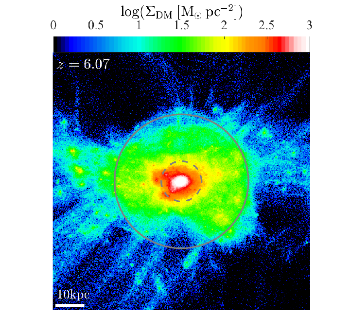
In order to illustrate some of the concepts discussed above, we show in a snapshot of a cosmological zoom-in simulation from the VELA simulation suite [25, 171]. The simulation was run with the adaptive-mesh refinement (AMR) code ART [102, 100, 24]. The code incorporates gas and metal cooling, UV-background photoionization with self-shielding in gas with Hydrogen number densities , stochastic star formation, gas recycling, stellar winds and metal enrichment, thermal feedback from supernovae [23] and feedback from radiation pressure [25]. The grid is refined using a quasi-Lagrangian strategy based on the total mass within a cell, up to a maximal resolution of (physical) at all times, though the resolution in the outer halo can be significantly lower. Details regarding the simulation method and its limitations can be found in Mandelker et al. [113]. In we show galaxy V19 (see table 1 of 113) at . At this time, V19 has a virial mass of , a virial radius of , and a stellar mass within of . The last significant merger was a merger at , roughly before the snapshot shown.
In , we show maps of the surface density of dark matter (left), gas (centre), and stars younger than (right). The panels in the top and bottom rows are and across respectively. Concentric solid and dashed circles mark and respectively. The integration depth of all panels is , and they are oriented perpendicular to the angular momentum of the central star-forming disk (see 113 for details on defining this plane). There are three prominent gas streams extending beyond the halo virial radius which seem to lie in a plane, the “stream plane”. While the existence of such a plane is a generic feature in cosmological simulations, it does not typically coincide with the plane defined by the disk angular momentum as it does in this case [37]. These gas streams lie at the centres of much wider dark matter filaments. The dark matter filaments are difficult to detect within the virial radius, while the gas streams remain prominent and coherent until reaching the interaction region at .
III. Fragmentation and Star-Formation in Streams
III.1. Stream Fragmentation in Cosmological Simulations
Several previous studies have addressed the possibility of clumpy accretion along streams and its potential effects on galaxy formation and disc instability [40, 42, 72, 77, e.g]. Other studies addressed the possibility of clumps forming due to thermal instabilities in massive halos or in streams and its potential effect on heating the CGM in proto-clusters [39, 10]. However, the formation of baryonic clumps within streams that are not associated with dark matter halos has not been studied in cosmological simulations (though 130 do show one such example). In , there are several dense clumps in the gas streams in the inner that do not appear to be associated with dark matter sub-halos. Two such clumps are highlighted with circles in the bottom panels. These clumps are forming stars despite not being associated with any dark matter overdensities.
In order to verify to what extent the highlighted clumps are devoid of dark matter, we show in the cumulative mass profiles of gas, stars, young stars (age ), and dark matter of the left-hand clump (hereafter clump 1) in . The corresponding profiles for the right-hand clump (hereafter clump 2) are qualitatively similar. The profiles are centered on the peak of gas density and extend out to the tidal radius of the clump. The tidal radius of a clump falling on a radial trajectory into a massive halo is given by the implicit formula [157]
| (1) |
where is the total mass of the clump interior to the clumpcentric radius , is the distance of the clump from the center of the host halo, and is the total mass of the host halo interior to the radius . The deprojected distance of clump 1 from the halo center is , and its tidal radius is . The total mass profiles interior to are shown in as thin dot-dashed lines. We then estimate for each gas cell, stellar and dark matter particle within whether or not it is bound to the clump, by comparing its velocity to the escape velocity from the cell/particle position to the tidal radius,
| (2) |
The profiles of bound mass are shown in as solid lines. There is no dark matter bound to the clump. The total mass profile of dark matter roughly scales as , indicating a constant background of dark matter from the host halo. On the other hand, over of the gas and stellar mass interior to is bound. The total bound baryonic mass of the clump is and its half mass radius is . Within this radius, all of the gas and over of the stars are bound, and the mean density is . The mass-weighted mean stellar age of the clump is , yielding an average SFR of .
In we show the mass-weighted metalicity of the gas phase in the same projection as the bottom panels of . Within the cold streams the typical metalicities are , consistent with observed metalicities of MP GCs. Similarly low metalicities have been found in the simulations analyzed by Fumagalli et al. [71], van de Voort & Schaye [158], Ceverino et al. [26]. The mass-weighted mean stellar metalicity within clump 1 is .
Clump 2 is qualitatively similar to clump 1. It has a tidal radius of , within which all the dark matter is unbound, while of the gas and stars are bound. Its gas mass is , similar to clump 1, but its stellar mass is only . Its mean stellar age is , younger than clump 1, with a mean stellar metalicitiy of .
We stress that we are not claiming that these specific clumps represent MP GCs, which we have no hope of resolving in these simulations. In fact these clumps disrupt as they approach the central galaxy, depositing some of their stars in the halo and some of them in the disc. However, these examples highlight the fact that gas streams may become unstable and form stars and stellar clusters far from the centre of any dark matter halo. Beyond the origin of MP GCs, this can have implications for the build-up of stellar halos around massive galaxies, and for the frequency of Ly emitters around massive galaxies at high redshift [58].
III.2. Observational Evidence
There is preliminary observational evidence for the fragmentation of cold streams. Radiative transfer models that attempt to reproduce the emission spectra of extended Lyman- nebulae around luminous quasars at in halos of mass , indicate that a large amount of gas is distributed in dense, compact clumps out to distances of at least [21, 3, 13]. Assuming that the emission is powered mainly by photoionization from the central quasar, the models place limits on the clump properties, suggesting densities of , sizes , temperatures , metalicities , and typical velocities of . While such clumps would be unresolved in cosmological simulations, we note that the mean density found in clump 1 () is of the same order. Under these conditions, hydrodynamic instabilities induced by the motion of these clouds through the hot halo gas should disrupt them on very short timescales [3]. This tension may be alleviated if the clumps are not travelling within a hydrostatic hot halo, but rather within an inflowing cold stream. It has been argued that such clumps may originate from Kelvin Helmholtz Instabilities (KHI) [114, 129], Rayleigh Taylor Instabilities (RTI) [93], or thermal instabilities [35]. Alternatively, they may be due to turbulent fragmentation in the streams (§IV.2).

Several recent observations highlight the possibility of star-formation occuring inside cold streams. Recent MUSE observations of a QSO, hosting a black-hole with an Eddington ratio of , have revealed the presence of a Ly nebula out to distances of from the QSO [58]. This is of the virial radius of a halo at (eq. 7). The inferred hydrogen volume density in the nebula is , similar to the densities in streams near at predicted by our model (eq. 24). Furthermore, the authors detected a Ly emitter (LAE) at a projected distance of from the QSO, with a line-of-sight velocity difference of , comparable to the virial velocity of a halo at (eq. 8), located along the direction of the extended nebula. The inferred SFR in this LAE is . Based on the QSO-galaxy cross-correlation function, the authors estimate that the probability of finding such a close LAE is . However, such a structure is a natural outcome of our model of star-forming clumps in gravitationally unstable streams, as detailed below. A similar example has been observed in an extended LAE near a bright QSO at [139], where it was speculated that feedback from the central QSO triggered a burst of star formation at an inferred rate of in a nearby dwarf galaxy roughly away from the QSO. We posit that such bursts of SF may occur directly in the dense, cold gas accreting onto galaxies without the need for a satellite dark matter halo or the “trigger” from a QSO.
Finally, ALMA observations of a very massive, , galaxy at reveal a large structure of molecular gas extending out to from the galaxy center [74]. This structure has a gas mass of , about of which does not appear to be associated with either the central galaxy or its satellites. Such a large molecular gas mass cannot be accounted for by tidal stripping of satellite galaxies, and kinematic analysis does not reveal coherent rotation in the extended structure. This extended structure is also detected in continuum thermal emission, with an inferred SFR of . The authors further detect gas rich systems on scales of up to oriented along the same direction as the extended molecular source, with gas masses in the range and SFRs of . The authors interpret these results as gravitational collapse and fragmentation leading to star-formation in the dense inner part of a cold stream feeding the central galaxy. A similar finding was reported in the Spiderweb galaxy, a massive proto-cluster at observed with the Australia Telescope Compact Array (ATCA) and the VLA [53]. These authors detected of star-forming molecular gas within an extended Ly- halo up to distances of from the central galaxy.
IV. Analytic Estimates of Stream Fragmentation
Motivated by the results of the previous section, we present in this section an analytical study of gravitational instability and fragmentation in cold streams. In §IV.1 we estimate the characteristic sizes and densities of cold streams. In §IV.2 we identify several sources of turbulence in the streams and estimate the resulting turbulent Mach numbers. In §IV.3 we assess the gravitational stability of streams and their characteristic fragmentation scales. In §IV.4 we discuss cooling below and estimate when star-formation can occur in the collapsed clouds. Finally, in §IV.5 we combine all the previous aspects of the model to assess when it may be possible to form MP GCs in streams. In the next section, §V, we summarize the main aspects of our model and highlight specific predictions for the properties of individual MP GCs and GC systems. A schematic illustration of our model, , and a table summarizing the main model parameters, Table 1, is presented here. Throughout, we normalize our results to streams feeding a halo at , which corresponds to the main progenitor of a halo at , i.e. a Milky-Way progenitor (). However, our model applies to all halos with , and we provide scalings with halo mass and redshift for all derived quantities.
IV.1. Characteristic Densities and Sizes of Cold Streams
We assume that the mass flux along the streams, which have a cylindrical or conical shape, is constant along their length until they reach the central halo [40, e.g.]. We thus have
| (3) |
where is the mass flux along the stream, is the stream radius, is its density, its velocity, and is the mass per unit length of the stream, hereafter the line-mass. As detailed below, we allow the stream density and radius to vary with radial position within the halo.
At , the mean accretion rate of total mass (baryons and dark matter) onto the virial radius of a halo with mass at redshift is well fit by11 1 While eq. (4) may slightly underpredict the accretion rate at [161], we note that a nearly identical formula can be derived analytically in the EdS regime at [43]. [54]
| (4) |
where and . The baryonic accretion rate onto the virial radius is given by multiplying eq. (4) by the universal baryon fraction, . At the high redshifts we are discussing we may assume that the accreted baryons are all gas. Cosmological simulations indicate that up to of the accretion onto the halo is carried by one dominant stream, with typically two less prominent filaments carrying up to each [37]. While these simulations focussed on halos at , we assume that similar fractions apply in stream fed halos at all redshifts. We adopt as our fiducial value for the fraction of the total accretion carried by a typical stream, and obtain for the gas accretion rate along such a stream
| (5) |
where and we have used . Fluctuations in the total accretion rate, namely in the normalization of eq. (4), can be absorbed into yielding a plausible range of [43].
The flow velocity along the stream may be written as
| (6) |
where is the virial velocity of the halo, and is an effective “Mach number”, defined as the ratio of the stream velocity to the halo virial velocity. Cosmological simulations indicate that the streams maintain a roughly constant inflow velocity slightly below the virial value as they travel through the halo [40, 76]. We assume , with an uncertainty of a factor of . The virial radius22 2 We define the halo virial radius as the radius of a sphere with mean density times the mean Universal matter density, valid at . and velocity of dark matter halos at are given by [43, e.g.]:
| (7) |
and
| (8) |
Eq. (3) can be combined with eqs. (5)-(8) to yield the typical line-mass of streams feeding a halo with virial mass at redshift :
| (9) |
The line-mass of the host dark matter filament is given by dividing eq. (9) by the Universal baryon fraction,
| (10) |
The characteristic radius of dark matter filaments as a function of their line-mass and redshift may be estimated by considering the expansion, turnaround and virialization of cylindrical top-hat perturbations in an expanding matter dominated Universe. This is analogous to the spherical collapse model for dark matter halos. Using this model, Fillmore & Goldreich [63] derived the trajectories of collapsing cylindrical shells. They found an overdensity of within the cylinder at turnaround (in the spherical collapse model, the overdensity at turnaround is ), and that complete radial collapse of the shell occurs at roughly times the turnaround time (as opposed to twice the turnaround time in the spherical collapse model). However, Fillmore & Goldreich [63] did not discuss virialization of the filament. The virial theorem per unit length for an infinite cylinder is
| (11) |
where is the kinetic energy per unit length and is the mass per unit length [29, 128]. Together with the expression for the gravitational potential at radius outside a cylinder with line-mass ,
| (12) |
where is a reference radius, one obtains a ratio of between the virial radius and the turnaround radius in the cylindrical collapse model (this ratio is in the spherical collapse model). This yields a virial overdensity inside the collapsed cylinder of33 3 Harford & Hamilton [80] quote a virial overdensity of , which is what one would infer if one assumes that the ratio of virial radius to turnaround radius for collapsed cylinders is , as it is for spheres. . The mean density in a virialized filament is thus
| (13) |
where is the critical density of the Universe at . Combining this with eq. (10), yields the virial radius of a dark matter filament,
| (14) |
The resulting ratio of filament radius to halo virial radius is
| (15) |
The relative width of filaments becomes smaller at later times, and has a very weak dependence on halo mass. For a halo at , this is roughly consistent with the most prominent filament seen on the left hand side of . For a halo at , the typical ratio is , which appears consistent with high-resolution cosmological zoom-in simulations [36, 126, e.g.].
The gas streams are significantly narrower than the dark matter filaments, since efficient cooling allows the gas to collapse towards the filament axis [38, 11]. However, the final radius of the gas streams and the mechanism that supports them against gravity has not been studied in detail yet. We expect the collapsed stream to be supported by a combination of thermal and turbulent pressure (see below), and rotation as evidenced by vorticity in the filament [32, 33, 108, 11]. Self-consistently modelling all these sources of support is beyond the scope of the current paper, and will require detailed simulations of stream evolution. In appendix §A, we show that assuming no rotation in the streams, equivalent to assuming that the streams are built by purely radial accretion of gas onto the centers of dark matter filaments, yields results that are inconsistent with both cosmological simulations and observations. Here, we adopt the opposite extreme and assume that the streams are largely supported by rotation, as has been suggested in the literature [11, e.g.]. This allows us to gain a crude estimate of the plausible sizes of streams, which turns out to be much more consistent with simulations and observations.
We assume that the stream radius, , scales with the radius of the dark matter filament via a contraction factor, ,
| (16) |
We further assume that the dark matter filament can be approximated as an isothermal cylinder truncated at . The density profile of an isothermal cylinder is [128]:
| (17) |
where is the central density of the filament, and is its half mass radius. The filament line-mass profile is
| (18) |
Inserting eq. (17) yields
| (19) |
where is the total line-mass of the filament. The associated circular velocity profile is
| (20) |
with the circular velocity at . This can be related to the filament virial velocity using eq. (11), yielding . If we assume that the specific angular momentum of the gas, , is conserved during the gas contraction and that it is similar to that of the dark matter in the virialized filament, then
| (21) |
where is the filament spin parameter, defined here analogously to the halo spin parameter of Bullock et al. [20]. We denote44 4 is analogous to the concentration of spherical dark-matter halos. , and thus . If eq. (21) reduces to
| (22) |
This yields , or for , , or respectively. Eq. (22) relates the stream contraction factor to the filament spin parameter. It has been known for some time that the spin parameter of dark matter halos has a constant average value of , independent of mass or time [20]. We assume that the filament spin parameter is likewise independent of mass or time, but with a smaller average value since the angular momentum of dark matter halos is predicted to originate from the combined angular momentum of the filament spin and orbit (impact parameter with respect to the halo centre) [151, 36, 108]. For and , we have . We hereafter assume as our fiducial value , but caution that this is highly uncertain and could easily vary by a factor of a few.
Cosmological simulations indicate that the streams assume a conical shape within the halo due to the gravitational attraction towards the halo center [40, 158, e.g.]. We thus assume within the halo, where is the halocentric radius. Together with eqs. (14) and (16), this yields an expression for the stream radius,
| (23) |
where and . This is comparable, within a factor , to the size of the large stream seen in . We note that in shock-heated halos with streams with radii are not expected to reach the central halo, since they will be shredded by KHI [114, 129]. This yields a practical lower limit of in such massive halos.
Eq. (23) can be used together with eq. (9) to obtain the average Hydrogen number density in the streams55 5 For a primordial composition of Hydrogen and Helium, the corresponding mass density in the streams is roughly .,
| (24) |
which is independent of halo mass. At , the position of clump 1 in , this yields a density of , comparable to the density within the half mass radius of the clump, where all the gas is still bound (). When scaled to , eq. (24) yields densities that are comparable to gas densities found in streams in cosmological simulations, which are in the range [78, 60, 158].
Combining eqs. (23) and (24) we can estimate the column density in a typical stream,
| (25) |
For a halo at , this corresponds to a surface mass density of , within a factor of 2 of the typical gas surface densities in the streams in . Given their high column densities, the streams should be mostly self-shielded against the mean UV background radiation at all times. This has been found in simulations at [78, 60].
IV.2. Turbulence in Streams
In this section we try to estimate the turbulent velocities and turbulent Mach numbers in the streams. The temperature of the stream gas is , near the Lyman cooling floor, [38, 11]. The isothermal sound speed is thus
| (26) |
where , is Boltzmann’s constant, and is the mean molecular weight, with the proton mass. The chosen value for is valid for a nearly primordial composition of neutral gas. can vary in the range [78], absorbing any possible variation in as well.
The first source of turbulence we consider is accretion of gas onto the streams from the large-scale pancakes within which they are embedded [169, 37], driven by the gravity of the streams and their host dark matter filaments. It is well established that such accretion generates turbulence [98, 86, 30, 85]. Based on the models of Klessen & Hennebelle [98], Heitsch [86] predicted the level of accretion driven turbulence in cylindrical filaments to be
| (27) |
where is an efficiency parameter which is inversely proprtional to the density contrast between the filament and the accreting material [98], is the accretion velocity onto , and is the mass accretion rate onto the stream.
We estimate the expected radial accretion velocities onto the cold streams by considering the free-fall velocity of a cylindrical gas shell starting from rest at the cylindrical turnaround radius, (§IV.1). Note that even if the gas has some net rotation velocity, as argued in §IV.1, we are here only interested in the radial component. At the gas is accelerated due to a constant line-mass , which is the total line-mass of the filament. The radial velocity at is
| (28) |
where we have used eq. (12) for the gravitational potential outside a filament with line-mass . is the virial velocity of the dark matter filament (§IV.1). At , the line-mass as a function of radius is given by eq. (19). This can be used to compute the change in potential from to and thus the radial velocity at :
| (29) |
where we recall that and . For our fiducial value of and , we obtain . Inserting eq. (10) into eq. (29) yields
| (30) |
It is striking that at this is comparable to the virial velocity of the dark matter host halo, though it declines more rapidly with redshift. We note that the actual infall velocity onto the streams may be smaller that the free-fall velocity computed above if there is some dissipation mechanism acting on the gas as it flows towards the filament axis. Since in eq. (30) is a factor larger than the virial velocity of the dark matter filament, this uncertainty should be within a factor of and can be absorbed into the efficiency parameter , discussed below.
The accretion rate onto the stream can be obtained by taking the time derivative of eq. (9) and inserting eq. (4) and the relation . The result is
| (31) |
where the expression in square brackets is for the halo masses and redshifts we are considering. Dividing eq. (31) by eq. (9) yields the specific accretion rate of gas onto the stream,
| (32) |
Since , where is the density of the accreted gas, we may combine eqs. (23), (24), (30), and (31) to obtain the density contrast between the accreted gas and the stream gas:
| (33) |
Inside the halo, the stream gas is times denser than the accreted gas. This appears roughly consistent with a visual impression from cosmological simulations [e.g. 37, figure 7]. Using numerical simulations and analytical arguments, Klessen & Hennebelle [98] found that the efficiency of converting the inflow kinetic energy to turbulent kinetic energy, from eq. (27), is approximately , with an uncertainty of a factor of . We adopt as our fiducial value a somewhat conservative . Inserting this along with eqs. (30) and (32) into eq. (27) yields an estimate for the turbulent velocities driven by accretion
| (34) |
where . Dividing by the sound speed (eq. 26) yields the turbulent Mach number associated with accretion
| (35) |
For our fiducial parameters at in the outer halo (), the resulting turbulent Mach numbers for halos of mass , , and are , , and respectively. Only for the most massive halos is the turbulence highly supersonic. In the inner halo, near , these values decrease by a factor of . At the turbulence is transonic for even the most massive halos.
In addition to accretion, there are several other potential sources of turbulence in the streams. As mentioned in §II, in massive halos with that contain hot gas at the virial temperature, the streams are susceptible to KHI caused by their interaction with the halo gas. The KHI results in oblique shocks within the stream that drive turbulence with Mach numbers of order [129]. In the inner halo, cold streams in hot halos may also be unstable to RTI provided they have an impact parameter with respect to the halo centre, placing them above the low density gas in the potential well [93]. Finally, cold streams in hot halos may also be thermally unstable [35], which can drive highly supersonic turbulence. We note that even in less massive halos, these processes may become relevant near the halo centre where hot gas ejected from the central galaxy due to feedback may form a hot corona [146].
Another source of turbulence and instabilities in the streams is satellite galaxies flowing along the streams towards the central galaxy. Simulations suggest that up to of the accretion into massive galaxies at is associated with such satellite galaxies in the form of both major and minor mergers [40]. These galaxies can locally stir up the gas in the streams, due both to their gravitational influence on and relative velocity with respect to the stream gas, potentially inducing large turbulent motions. Furthermore, winds ejected from these satellite galaxies into the stream gas can cause shocks and stir up turbulence, and have a profound influence on the structure of streams [59].
Altogether we estimate that instabilities and feedback can drive turbulence in the streams with Mach numbers of to a few, preferentially in massive halos with . When summed in quadrature to turbulent velocities driven by accretion, the turbulent Mach numbers in streams near may reach , and in halos of mass , and respectively at . However, by these values should decrease by .
IV.3. Gravitational Instability and Fragmentation
Self-gravitating filaments are unstable to local perturbations at wavelengths larger than the 3d Jeans length, provided this is smaller than the radial scale of the filament, even in the presence of rotation [69]. The Jeans length is given by
| (36) |
where represents the combined radial support due to thermal and turbulent pressure. Based on the discussion in the previous section, we have , , and for streams in halos of mass , and respectively at . At lower redshifts, the contribution of turbulent support decreases further. Therefore, in the following discussion we simply adopt , and comment where relevant on how this may underestimate the resulting fragmentation scales. This has the advantage of examining the degree to which thermal pressure alone can support the streams against fragmentation, since streams are often modeled in the literature simply as isothermal cylinders at [38, 80, 114, e.g.].
Using eqs. (23), (24) and (26) we may compute the ratio of the thermal Jeans length to the filament diameter,
| (37) |
Note that this is independent of and of position within the halo. For a halo, a stream carrying of the total accretion has a thermal Jeans length equal to the stream width. For more massive halos , which means that local density perturbations can trigger gravitational collapse within the streams. It can easily be verified that adopting the turbulent Jeans length does not change this conclusion. For streams where , the characteristic mass of gravitationally unstable clumps is given by the Jeans mass,
| (38) |
Note that the thermal Jeans mass is independent of halo mass, and scales linearly with halocentric radius. At , the turbulent Jeans mass is larger by a factor of and in streams feeding halos of mass and . At lower redshifts the difference between the thermal and turbulent Jeans masses becomes smaller. In appendix §B we show that the effects of the tidal fields induced by the host halo and the host dark-matter filament on the fragmentation scale are both negligible.
In order to ascertain whether such a Jeans unstable cloud will have time to collapse before the stream reaches the central galaxy, we compare the free fall time, , to the inflow time from a given radius, . We find
| (39) |
This is independent of halo mass, redshift, or position within the halo. Wherever the perturbation is seeded, it will collapse in roughly half the time it takes to reach the central galaxy.
For long wavelength perturbations, larger than the filament diameter, the above local stability criterion cannot be used, and we must instead examine the global stability of the filament. A self-gravitating isothermal filament is unstable to global axisymmetric perturbations if its line-mass is larger than a critial value [128, 90, e.g.]. This can be thought of as a filamentary “Jeans line-mass”, above which thermal pressure cannot prevent global radial collapse of the filament. The ratio of the line-mass in a typical stream to this critical value is
| (40) |
At , streams feeding halos more massive than are supercritical, and thus globally unstable. At , the critical halo mass for unstable streams is , smaller than at that redshift (). The characteristic collapse time for a supercritical filament is [90, 86]. Comparing this to the inflow time we find
| (41) |
so the stream has time to globally fragment before reaching the central galaxy. This global instability results in the formation of dense cores separated by a few times the filament diameter [90, 31]. These cores then proceed to fragment on the local Jeans scale discussed above [31, 30].
Our analysis thus suggests that most streams are supercritical with fragmentation times shorter than the halo crossing time. This is exacerbated further by the additional inwards gravitational force of the dark matter filament. This means that there must be some additional source of support in the streams which prevents catastrophic fragmentation in cosmological simulations. This could be rotation (§IV.1), turbulence (§IV.2), or artificial support caused by low resolution. However, Heitsch [86] found that accretion-driven turbulence, which we expect to be the dominant source of accretion in most cases, can slow down the global collapse of supercritical filaments but it cannot halt it. The basic reason is that the line-mass of the stream grows faster than the resulting turbulent support, and therefore the stream remains super-critical. This has been confirmed by Clarke et al. [30], who simulated a self-gravitating isothermal filament growing by accretion from its surroundings. They found that as long as the accretion flow itself was not highly turbulent, gravitational collapse and fragmentation occurs in two stages, first on large scales set by filamentary fragmentation, and then on small scales set by the local Jeans scale.
To summarize, we find that most streams feeding massive halos should be gravitationally unstable to both short and long wavelength perturbations. The former result in direct three dimensional collapse on the Jeans scale, of clouds with masses given by eq. (38). The latter result first in two dimensional filamentary collapse, followed by subsequent three dimensional collapse on the Jeans scale, leading to collapsed clouds with the same mass as in the former case. Both of these processes can act in less than a virial crossing time, particularly if the stream is relatively narrow with .
IV.4. Cooling and Star Formation
In order for star-formation to occur in the collapsing gas clumps, they must be able to cool from the initial stream temperatures of down to . If the streams are indeed self shielded against the UV background then at they are mostly neutral, as assumed above. At metalicities of , and at the characteristic densities and temperatures of the streams, the dominant cooling process is emission in the line [107, 130]. For a cloud of gas with a mean Hydrogen number density , metalicity , temperature , and clumping factor , the ratio of the cooling time to the free-fall time of the cloud is [107, equation 6]
| (42) |
For a collapsing cloud, this ratio decreases as the density increases during the collapse. However, since both the free-fall time and the cooling time are dominated by their initial stages near the onset of collapse, this initial ratio is representative of the final ratio. Inserting eq. (24) for the mean density in the streams and using this yields
| (43) |
Note that this depends on position in the halo through the stream density.
Multiplying eq. (43) by eq. (39) yields the ratio of cooling time in the streams to the inflow time,
| (44) |
This ratio increases towards lower redshifts, as the streams become less dense. We define the cooling redshift, as the redshift where the cooling time is equal to the inflow time,
| (45) |
At , the cooling time in the collapsing clump is longer than the inflow time to the halo center, and we do not expect much star-formation in the clump. However, at , the clump may experience a burst of star-formation before reaching the central galaxy.
Clumping factors of are not unreasonable at given the levels of turbulence and substructure in the streams. In fact observations suggest that the clumping factors may be even higher in very massive halos (§III.2). We therefore assume at , possibly approaching for halos where the turbulent velocities are very large. However, as the turbulent velocities decrease towards lower redshift the associated clumping factors may decrease as well. For a relatively narrow stream with near the inner halo at , with a metalicity of () and a clumping factor of , this yields . At , this yields . In this case, the clump can cool and proceed to star-formation on a free-fall timescale, before reaching the central galaxy. Furthermore, since the initial cooling timescale is longer than the free-fall timescale of the cloud, we expect relatively large contraction factors for these clouds before the onset of star-formation. This can increase the mean densities in the clouds by considerable amounts compared to the mean densities in the streams given by eq. (24). It is also worth noting that such a cloud can cool and form stars before forming any appreciable fraction of [107].
In order to obtain in a stream with fiducial parameters, we require either larger metalicities closer to , or larger clumping factors. Overall, we predict star-formation to be less likely to occur in the streams outside the central galaxy at , unless the metalicities are , larger than indicated by most cosmological simulations [71, 158, 26].
In order for collapse to occur the clump must also dissipate its turbulent support. The initial clump radius is of order the stream radius (eq. 37). When accounting for turbulence in the Jeans length, this remains true even at . The dissipation rate of turbulence over a length scale is equal to . Using eq. (34) as a proxy for the total turbulence in the clump, the ratio of this timescale to the inflow time can be evaluated:
| (46) |
For a typical stream, the initial turbulence will dissipate in roughly the time it takes the stream to reach the central galaxy. At the ratio increases to for , but if it is .
IV.5. Formation of MP GCs

IV.5.1 Gas Pressure in Streams
We have established that streams at high redshift are unstable to fragmentation and that the cooling time is short enough to allow star-formation in the collapsing gas clouds. In order to form GCs in the collapsing clouds, they must reach high enough densities and pressures. GCs are expected to form only in very high pressure regions, with [51, 105]. The combined thermal plus turbulent pressure in the streams prior to gravitational collapse is given by (see §IV.3). This is shown as a function of halo mass and redshift in . We assumed fiducial values for the stream velocity and temperature, the fraction of total accretion in the stream, and the efficiency of converting accretion energy into turbulent energy. In other words, . However, we assumed a relatively narrow stream, with . The turbulent Mach number is given by from eq. (35), summed in quadrature with an additional to account for instabilities and feedback (see §IV.2). The white lines in represent mass evolution tracks of halos with masses , and .
For the chosen parameters, the pressure in the streams exceeds at for all halo masses, and at for the progenitors of the most massive halos, . Recall that the pressure plotted in , which represents the pressure in the streams prior to gravitational collapse, is not enough to maintain the streams in hydrostatic equilibrium when (eq. 40). The final pressure in the collapsed clouds prior to the onset of star-formation is thus likely to be even higher. We conclude that at the pressure in the streams in the inner halo is large enough to enable formation of GCs. However, this may not be true outside of due to the strong dependence of the density and pressure on position within the halo, .
IV.5.2 Cluster Formation Efficiency
In addition to large pressures, the formation of a GC requires very high densities. A typical GC with a mass of and a half-mass radius of has a mean density within this radius of . At , at , even a relatively narrow (and thus dense) stream with has a typical density of according to eq. (24), roughly a factor of 2000 below the densities in GCs. However, we cannot compare the mean density in the stream or in the pre-collapse cloud to the final GC density. Star-formation in a turbulent medium is a hierarchical process where the densest objects, namely bound stellar clusters and GCs, form at the highest density peaks within the cloud [106, 87, e.g.]. Furthermore, there is mounting evidence in the local Universe that the densest stellar clusters are significantly denser than the densest gas clouds [112, 165], suggesting that massive clusters are formed via hierarchical merging of smaller stellar clusters embedded in the parent gas cloud.


Within this framework, one can evaluate the fraction of star-formation occuring in bound clusters, referred to as the cluster formation efficiency, or CFE [6, 75, e.g.], based on the density and pressure within the parent cloud66 6 There is still some debate in the literature regarding the origin of the CFE, with some claiming that it does not depend on the properties of the host galaxy or of the parent cloud [55, 27, 28, 124]. However, we here adopt the theoretical framework of Kruijssen [103] whereby the CFE depends on the density and pressure in the parent cloud. [103, 1, 92]. For a halo at with the same parameters as in , the streams have pressure , density , and column density . These properties are very similar to those of the Fornax model of Kruijssen [105] (Table 1), which had , , , and a CFE of . In our model, the density and pressure in the collapsed clouds prior to the onset of star-formation are likely to be much higher than the typical stream values, so CFE values of or larger are entirely plausible.
The CFE can be used to determine the maximal cluster mass that forms within the parent cloud, where is the fraction of the cloud mass that turns into stars [140]. For , , and (eq. 38), we infer a maximal cluster mass of order which is again consistent with the maximal cluster mass in the Fornax model of Kruijssen [105]. For halos with at , which are the progenitors of halos at , we expect larger CFE values due to stronger gravitational instability as well as larger Jeans masses due to stronger turbulence (see §IV.3). Both of these will yield larger cluster masses.
IV.5.3 Dense Gas Fraction
Notwithstanding the above discussion, we defer a more detailed evaluation of the CFE and the maximal cluster mass in streams to future work, focussing here instead on the simpler question of under what conditions a collapsed cloud will have enough gas at high enough densities to lead directly to the formation of a GC. Based on the above discussion, this is a sufficient but not necessary condition for GC formation. As previously stated, a typical GC is times denser than a typical stream. For the mean density in the collapsed cloud to reach these values, a radial contraction factor of is required, where is the radius of the collapsed cloud. At lower redshifts and at larger halocentric distances, the discrepancy is larger. While we have argued in the previous section that the relatively long cooling times in the clouds compared to their free-fall timescale can lead to significant contraction factors before the onset of star-formation, a contraction factor of may still be difficult to achieve due to angular momentum support.
However, as described above it is not necessary for the mean density in the cloud to be as dense as a GC, but only that the highest density peaks are dense enough. The volume-weighted PDF of the mass overdensity in an isothermal turbulent medium is well described by a lognormal distribution [62, 99, e.g.]
| (47) |
where is the overdensity, and
| (48) |
where is the turbulent Mach number, and depends on the ratio of compressive to solenoidal modes in the turbulence. For a “natural” mixture of modes , while it approaches for more compressive forcing [62]. We can use this expression to estimate the fraction of mass that will be dense enough to form a GC, i.e. .
We assume that the cloud begins with mean density (eq. 24) and then contracts radially by a factor of , so that its final density is . The turbulence in the initial cloud is given by from eq. (35), summed in quadrature with an additional to account for instabilities and feedback, as in . As the cloud contracts, its internal turbulence may be amplified. In the absense of any dissipation or cooling, , so the turbulent Mach number scales as . However, in practice this maximal enhancement is rarely seen in simulations since turbulence dissipates more rapidly as the cloud contracts. As a conservative estimate, we ignore the possible enhancement of turbulence and assume that it remains constant during the contraction. This may result in an underestimate of the dense gas fraction.
In , we show the fraction of gas in the collapsed cloud which is denser than as a function of halo mass and redshift. The different panels explore different values of the contraction factor, and , and the halocentric distances, and . All other parameters are the same as in , namely and . The vertical dashed line shows from eq. (45), assuming a clumping factor of and a metalicity of . The white solid lines in each panel represent halo mass evolution tracks, as in .
GCs are expected to undergo mass loss of a factor of from their formation until [105, 16]. The formation mass of a typical GC should thus be in the range . In practice, since our model predicts that GCs form directly in the halo rather than in the central disc, the actual mass loss may be on the low side [105], so a typical GC with mass at may have had a formation mass as low as . Nevertheless, we hereafter adopt the conservative estimate that the formation mass of a GC is , and require at least this much gas to be above . This can also allow for the formation of multiple clusters with a range of masses in a given parent cloud.
We can estimate the total mass of gas with by multiplying the fraction of dense gas shown in by the turbulent Jeans mass (see §IV.3). The black dotted line in each panel of marks the contour of of gas with in a collapsed cloud. Above this line, there is enough dense gas to form a GC. We see that in all cases, at this contour roughly corresponds to the contour of .
From the left-hand panel of we learn that in the outer halo, at , even with very large contraction factors of only the progenitors of halos at have enough dense gas to form GCs at . Even at , only progenitors of halos have enough dense gas to form GCs. We conclude that GC formation in streams is unlikely to occur in the outer halo, which was the same conclusion we reached when considering the pressure in the streams in .
From the center panel of we see that even in the inner halo, at , a contraction factor of will not result in direct collapse of a GC within the collapsed cloud, except in extremely massive halos with at .
In the right-hand panel of , we examine the case of and . In this case, . At , for all halos with , of the mass of the collapsed cloud has densities . Furthermore, there is enough dense gas in the collapsed cloud to directly form a GC with at . We conclude that if the collapsing clouds can reach contraction factors of , then MP GC formation will occur in cold streams in the inner of the halo, outside the central galaxy.
IV.5.4 Stream Collisions
What now remains is to ask whether such a large contraction factor is possible. As noted above, since the gas stream is at least partially supported by rotation, the cloud contraction will be limited by angular momentum support at some point. While the degree of angular mometum support, and thus the maximal contraction factor, are unknown, it seems unlikely that the clumps will be able to contract in size by a factor without losing some angular momentum. Fortunately, there is a natural mechanism for this in the inner halo. As described in §II, interior to the streams interact with each other and with the central disc as they form an extended rotating ring and spiral towards the central galaxy within an orbital time [36]. While most of the streams are co-rotating, thus efficiently transporting angular momentum to the growing disc, simulations indicate that of the mass flowing into this interaction region is actually counter-rotating [36]. A counter-rotating stream can collide with another stream in this region. Such a collision could significantly reduce the angular momentum of the stream and of the collapsing clouds, as required. Furthermore, the collision itself could significantly increase the densities of the collapsing clouds. The relative velocity of the collision is of the order of the stream velocity, , and thus has a Mach number of
| (49) |
The very short cooling times in the streams following such a collision should result in an isothermal shock (see 35 for a discussion on strong isothermal shocks in cold streams as they enter the virial radius of a hot halo), resulting in an increase in the stream density by a factor . For a halo at this is comparable to the density increase in a cloud with a radial contraction factor of , though for lower mass halos and lower redshift the density increase is smaller. The mean density in the collapsing clouds may increase by a similar factor as well, allowing GC formation at lower global contraction factors77 7 We note that this scenario bears certain qualitative similarities to the scenario proposed by Fall & Rees [56], except that here the dense clouds are confined by the ram pressure of stream collisions rather than the thermal pressure of a hydrostatic halo at the virial temperature, though both these pressures have comparable magnitudes.. We conclude that such stream collisions in the inner halo may act as the trigger for MP GC formation.
V. Summary and Predictions of the Model
| Model Parameters | ||||
|---|---|---|---|---|
| Parameter | Meaning | Reference eqn. | Fiducial Value | Plausible Range |
| Fraction of average halo accretion along a single stream | eq. (5) | |||
| Ratio of stream velocity to halo virial velocity | eq. (6) | |||
| Ratio of stream radius to dark matter filament virial radius | eq. (16) | |||
| Stream gas temperature | eq. (26) | |||
| Turbulence driving efficiency | eq. (27) | |||
| Clumping factor in the streams | eq. (42) | |||
| Stream gas metalicity | eq. (42) | |||

V.1. Stream Fragmentation
Figure 7 presents a schematic diagram highlighting the main ingredients of our model. Massive halos at high redshift are fed by cosmic web filaments of dark matter which contain dense streams of cold, , gas in their centers. Outside the halo the filaments and streams are roughly isothermal cylinders. Inside the halo the dark matter filaments mix in with the surrounding medium and virialize, while the streams remain cold and coherent as they penetrate towards the inner in a conical shape. This element of the model is not new, and has been discussed in several previous works [36, e.g.]. However, our model discusses in detail for the first time gravitational instability and fragmentation of the streams. Along the way, the streams become gravitationally unstable to both large-scale cylindrical instabilities and local Jeans instabilities. They fragment into bound clumps with masses in halos with . At high redshift, typically though possibly at lower redshifts if the metalicity is more than solar, these clumps can cool and form stars before reaching the central galaxy. This is seen in cosmological simulations (Figs. 2 and 3), and may have been observed in a few instances (see §III.2). Little or no dark matter is expected to be bound to these clumps despite their location at distances of up to tens of from the central galaxy. While many of these clumps may eventually be destroyed by the tidal forces of the central galaxy, they can contribute to the growth of the metal-poor population in the stellar halo (, ) and may be observed as Ly emitters.
There are seven parameters that define the various aspects of our model. These are summarized in Table 1, along with the equation where they first appear and with their fiducial values and plausible ranges, based on the arguments laid forth in §IV. The gravitational stability of cold streams depends on , , and , with faster, hotter and less prominent streams being more stable (eqs. 37 and 40). Pushing these to their extreme values, our model predicts that the minimal halo mass where streams are likely to be gravitationally unstable at is in the range , while for typical values halos with at should host unstable streams. Whether this instability is able to manifest itself in the halo, before the streams reach the central galaxy, depends primarily on the product (eqs. 39, 41, and 45). For typical values, clumps collapse and cool before reaching the galaxy, though if a stream is both very wide and rapidly inflowing this may not be the case. The thermal Jeans mass in the streams depends on stream width, , and on position within the halo (eq. 38). For the full range of plausible values and for halocentric distances of , the thermal Jeans mass is , though it is expected to typically be a few times .
The level of turbulence in the streams depends on the first five parameters in Table 1 (eq. 35). The turbulent Mach number increases for slower, wider, colder, and more prominent streams, with a larger driving efficiency. In our fiducial model, turbulence played a significant role only in the most massive halos, at , while for less massive halos and at lower redshifts thermal pressure dominated over turbulent pressure. Therefore, if the parameters are such that the turbulence is even lower, this will not alter our main conclusions. On the other hand, if we take extreme values for all parameters to make the turbulence as large as possible (, , , , ), the turbulent pressure can dominate even in halos. This would yield larger density and pressures peaks in the streams, thereby strengthening the case for globular cluster formation. However, such a parameter combination seems unlikely, and we do not expect turbulence to be significant in halos less massive than a few times .
Finally, the redshift above which the streams can cool to and form stars before reaching the central galaxy depends on the product of (as well as as described above, eq. 45). A stream with both very low metalicity and very small clumping factor will not be able to cool and form stars at as in our model. However, our fiducial clumping factor of is at the low end of the expected range, and cosmological simulations suggest that streams feeding massive galaxies have been enriched to roughly solar metalicity by , so we expect that for typical cases streams should be able to cool and form stars at . The plausible range for these parameters may even lead to cooling and star-formation at somewhat lower redshifts.
V.2. Globular Cluster Formation
At , in the inner for a relatively narrow (though by no means extreme) stream with , the pressure in the streams is large enough to enable GC formation (). The cluster formation efficiency (CFE) is expected to be , yielding maximal cluster masses of in halos with . The maximal cluster mass may increase by a factor of in halos with , both because of an increased turbulent Jeans mass and an expected increase of the CFE. These values are consistent with previous estimates of GC masses at formation in models where GCs form in dense GMCs within high redshift discs [105]. The low metalicity in the cold streams results in a low metalicity of for these clusters, similar to MP GCs. However, due to the strong dependence of the density and pressure on stream width, it is unlikely that regular star formation in the streams will result in GC formation for .
The inner consists of a messy interaction region where the streams join the disc. In this region, collisions between counter-rotating streams can result in densities and pressures large enough to form GCs even if (), and may be the dominant formation channel of MP GCs in our model. These proto-GCs may have masses of the mass of their parent cloud, namely a few times ( for the most massive halos), and be essentially devoid of dark matter. Their masses then decrease by a factor of by , yielding masses typical of observed GCs.
Our model may allow for formation of GCs at relatively low redshifts, down to for the progenitors of halos at , and down to for the progenitors of halos. The latter is assuming larger clumping factors due to larger turbulent velocities, in order to allow the collapsing clouds to cool before reaching the halo centers. This likely results in higher metalicities for the GCs formed in more massive halos, owing to the overall larger metalicities at lower redshifts. Additionally, those GCs that form at lower redshift form in more massive clouds (eq. 38). A trend between the mass of individual MP GCs and the mass of their host halo is indeed observed [81]. This is also qualitatively consistent with the observed correlation between the mass and metalicity of MP GCs, the “blue tilt”, since more massive halos at lower redshift will have higher metalicity gas. This feature is not observed for MR GCs [18, e.g.], possibly hinting at a different formation environment for the two populations.
The kinematics of the MP GC population is a result of the kinematics of the streams in the inner where we estimate fragmentation is most likely to occur. As discussed in §II, this is the region where the angular momentum is transferred from the streams to the disc due to strong torques, and the streams form an extended, high angular momentum, ring-like structure. Formation of MP GCs in these conditions may help explain the rapid rotation velocities and velocity anisotropies observed in the MP GC population in the outer halos [134].
Our picture of MP GC formation in the inner halo allows us to place constraints on two important observables: the ratio of the mass of a MP GC system (GCS) to that of its host halo at , and the ratio of the extent of a GCS to the virial radius of its host halo at . Both of these are observed to be constant over several orders of magnitude in halo mass [81, 64].

An upper limit to the total mass of the MP GCs that formed in situ in the host halo as a result of collisions between counter-rotating streams, rather than having been accreted at lower redshift, can be obtained as follows. As stated above, simulations indicate that of the gas mass entering is counter-rotating. We assume that all the counter-rotating gas that enters between an initial redshift and the redshift where from falls below , , contributes to formation of MP GCs at efficiency. At these high redshifts, the halo mass as a function of redshift is well approximated by [41]. For all halos of interest, . For a given , the fraction of mass accreted onto a halo in the redshift range is independent of halo mass. For , this fraction is . Thus the efficiency of GC formation relative to the total baryonic mass in the halo at is , independent of halo mass. In his empirical model of hierarchical merging of globular cluster systems, Boylan-Kolchin [16] found that formation efficiencies of for MP GCs in halos at , combined with GC mass loss by a factor of until , can account for the present day masses of GC systems.
If we assume additional mass loss by a factor of until , we have of the counter-rotating mass entering from to winds up in MP GCs at . Note that this represents mass loss from the entire GCS rather than from an individual GC, and thus includes GC disruption as well. This is of the total gas mass or of the total mass accreted onto the halo in this interval, where is the fraction of gas crossing the virial radius that penetrates down to . In halos with virial mass we expect , while in more massive halos we expect due to the presence of a hot halo out to the virial radius [43, 41]. This is only relevant for the progenitors of very massive halos with at , since lower mass halos are always less massive than at ().
In we show the results of this simple model for different values of , for the same model parameters as in the right-hand panel of . For each chosen we show the ratio of the total GCS mass to the host halo mass at as a function of host halo mass. The kink at in all model curves is due to the progenitors of these massive halos crossing the threshold at . For comparison we show the recent result of Harris et al. [81], who found a ratio of . For , our results for low mass halos with are in very good agreement with the observations, suggesting that a large fraction of their MP GCs could have formed via this mechanism. At higher masses we underproduce the total mass of the MP GCS. But this is to be expected, since we are only accounting here for MP GCs that formed as a result of stream collisions in the halo. The remaining GCs are ex situ in origin, accreted onto the halo during mergers of sub-halos88 8 As discussed, we also expect some MP GC formation in streams feeding massive halos even in the absense of collisions. The contribution of these clusters to the total population depends on both the CFE and the total amound of star formation in the streams, and will be the subject of future work.. We find that the fraction of mass in ex situ MP GCs accreted during mergers increases with halo mass, because more massive halos accumulated a larger fraction of their total mass through mergers of halos with at , the threshold for in situ MP GC formation in our model. For a MW mass galaxy, with , we find that of the total GC mass was formed in the halo of the main progenitor at . This is in good agreement with the estimates of Boylan-Kolchin [16] who constrained this value using halo merger trees. In his model, he assumed that every halo above at formed MP GCs in the halo with a total mass proportional to the halo mass at , but did not propose a physical mechanism by which this could occur. Our model provides such a physical mechanism, and forms the basis for formation of MP GCs directly in the halos of massive galaxies at . Hierarchical models can then be used to assess the accretion of ex situ GCs via mergers of sub halos.

In addition to the total mass, we can also place constraints on the radial extent of the in situ MP GCs by assuming that most MP GCs are formed at at , and remain at the same physical distance from the halo center at . Indeed, the dynamical friction timescale for a GC on a circular orbit at in a halo is , longer than the age of the Universe (9 equation 8.13, assuming a Coloumb logarithm of ). Figure 9 shows the results of this simple model in comparison to recent observations by Forbes [64]. The observational data show the half-number radii of GCs in a sample of GCSs spanning 3 orders of magnitude in halo mass, from , and including ultra-diffuse galaxies, giant ellipticals and the MW. This study found that the radial extent of GCs was proportional to the virial radius of their host halo, scaling as . However, we do note that Hudson & Robison [89] found a different, non-linear, scaling of the extent of GCSs with halo virial radius, albeit using a smaller sample than Forbes [64]. Further observations are needed to clarify this point. Comparing our simple model to the observations, we see that while we systematically underpredict the radial extent of GCSs by compared to the observations, the slope of the GCS size-halo mass relation is consistent with observations, including the steepening at . In our model, this steepening is due to decreasing below , towards and for and halos.
The larger observed radial extents of GCSs compared to our simple model indicates that ex situ GCs which are accreted onto the halo via mergers tend to lie at larger galactocentric distances than those that formed in situ. Furthermore, violent relaxation associated with halo assembly from to will mix the dark matter and GCs, possibly increasing the effective radius of the GCS. The maximal radius that can be reached by this process is the half-mass radius of the dark matter halo. In we show the effective radius of an NFW halo as a function of halo mass, assuming the mass-concentration relation of Zhao et al. [170]. The slope of this relation is similar to the observed slope, and the observed data are roughly midway between this upper limit and our estimated lower limit.
Finally, we stress that our model makes a testable prediction, namely that at high redshift during the epoch of GC formation, both MP GCs and less dense star-forming clouds should trace the streams that feed galaxies. They should reside outside galaxies, at distances of up to tens of , along filamentary, possibly ring like structures. Future observations with JWST are expected to observe the formation of GCs [142, 16], and will be able to test these predictions.
VI. Discussion and Proposed Future Work
We have presented a new model for the formation of metal-poor globular clusters (MP GCs), whereby they form in the dense streams of gas predicted to feed massive galaxies at high redshift. This is reminiscent of older models for the formation of MP GCs in the halos of massive galaxies at high redshift [56, 22], but accounts for our new understanding of the filamentary nature of the gas in these halos. The filamentary versus spherical structure leads to higher overall gas density thus fascilitating gravitational instability. We have shown that such streams are unstable to gravitational instabilities on both small and large scales, and that such instabilities can collapse in less than a halo crossing time. At high redshift, , the collapsing clouds can cool and form stars even if their metalicity is only . In the inner of halos at , the pressure in the streams is large enough to enable the formation of GCs. This is already true prior to the onset of gravitational instability, and will only be aided by gravitationl collapse. The mean densities and pressures in the streams at these redshifts are similar to those predicted for the ISM in a Fornax progenitor at [105], and imply a cluster formation efficiency (CFE) of in the streams. This value likely increases with halo mass due to increased turbulent pressure. This implies a maximal formation mass for GCs of in halos at , and up to an order of magnitude larger in halos. Additionally, collisions of counter-rotating streams in the inner can lead to very large compression in the clouds, resulting in enough gas at high enough densities to directly form a massive GC.
Our model very naturally accounts for numerous observed properties of MP GCs and GC systems. These include the lack of dark matter in GCs, the typical masses of GCs, the correlation between the mass and metalicity of MP GCs (as opposed to MR GCs), the correlation between the mass of individual MP GCs and the mass of their host halo, the kinematics of MP GCs in the halo, the correlation of the total mass of a MP GC system with the mass of its host halo rather than the stellar mass of the central galaxy, and the correlation between the radial extent of a GC system and the virial radius of its host halo. Other predictions, such as a spread in formation times for MP GCs between and a trend such that more massive, more metal rich MP GCs are younger, can be tested with future detailed observations that can increase the accuracy of age determinations for MP GCs. The key prediction of our model, that the progenitors of MP GCs should trace the streams in the halos around galaxies, out to distances of tens of , will be testable with upcoming JWST observations.
Despite the many attractive features of our proposed scenario, we highlight that at the moment the evidence is merely suggestive. In §IV we have attempted to make quantitative predictions regarding the structure and stability of cold streams and the substructure that may form within them, but these are only crude estimates. Our model demonstrates that the dense gas in cold streams is likely gravitationally unstable and can lead to the formation of stars and stellar clusters in the streams far from the central galaxy. This aspect seems supported by cosmological simulations and possibly by recent observations. However, we have not estimated the total expected SFR or CFE in the streams, nor have we shown that stream collisions in the inner halo will result in the formation of a GC. To properly address the latter, and to better understand the general process of gravitational fragmentation of streams in the halo, high resolution numerical simulations will be necessary, as detailed below. Additionally, our picture does not account at all for the MR GCs, which likely form inside galaxies [65, 145, 105] rather than in their halos. Our main purpose in this paper was to address the general concept of stream instability at high redshift, to highlight a mechanism for the formation of MP GCs directly in the halos of massive galaxies at high redshift, and to point to supportive evidence that this scenaro is feasible and can account for many observed properties of the MP GC population.
In order to test and refine some of our assumptions and conclusions, future detailed studies of streams will be necessary. One aspect of such studies should utilise large scale cosmological simulations to obtain statistics regarding the large scale properties of both dark matter filaments and their associated gas streams, such as their mass per unit length, radial size, and spin parameter, in much the same way as similar studies have been done for dark matter halos and galaxies. By studying such global properties of filaments and how they relate to the properties of the dark matter halos they feed, the predictions of §IV can be tested and refined. Additionally, in a follow-up paper we will examine the frequency and properties of star-forming clumps formed in the streams of the full VELA simulation suite.
The second aspect of future studies of cold streams requires detailed studies of the evolution and stability of these streams under various conditions. Since the resolution in streams in current cosmological simulations is limited [126], such studies require idealized simulations of isolated streams inside individual halos. A few such studies have been presented recently [114, 35, 129]. They have shown that streams may be unstable to both hydrodynamical and thermal instabilities, which may lead to supersonic turbulence within the streams and to their eventual fragmentation. However, the analysis presented in Mandelker et al. [114] and Padnos et al. [129], did not include cooling, the study presented in Cornuault et al. [35] included only analytical calculations with no simulations at all and neglected hydrodynamic instabilities, and none of these studies accounted for self gravity in the stream or the external gravitational potential of the dark matter halo. Additionally, it will be important to directly simulate the collision of counter-rotating streams, since this is predicted to be the main mechanism of GC formation in our model. These additional physics should be addressed in future work, which will enable the fundamental assumptions and predictions of the model presented here to be tested. Until that time, the model presented in this paper may serve as a qualitative guide to future studies of the stability of cold streams feeding massive galaxies at high redshift, the origin of MP GCs, and the relation between them.
Acknowledgments
We thank the anonymous referee for constructive comments which have improved the quality of this manuscript. We are greatly indebted to Avishai Dekel for inspiring large parts of this work, and for his continuous support. We thank Avishai Dekel and Joel Primack for the use of the VELA simulations. We gratefully acknowledge Avishai Dekel, Diederik Kruijssen, and Daisuke Nagai for their careful reading of and thoughtful comments on an earlier version of the mauscript. We thank Yuval Birnboim, Frederic Bournaud, Andi Burkert, Bruce Elmegreen, Kohei Inayoshi, Thorsten Naab, and Stefanie Walch for very helpful discussions. We thank Andrew P. Hearin for his help with the Colossus package used in creating . NM and FB acknowledge support from the Klaus Tschira Foundation, through the HITS-Yale Program in Astrophysics (HYPA). FB is supported by the US National Science Foundation through grant AST-1516962. JB acknowleges support from NSF grant AST-1616598. DC has been funded by the ERC Advanced Grant, STARLIGHT: Formation of the First Stars (project number 339177). The VELA simulations were performed at the National Energy Research Scientific Computing centre (NERSC), Lawrence Berkeley National Laboratory, and at NASA Advanced Supercomputing (NAS) at NASA Ames Research Center (PI: Joel Primack).
References
- [1] Adamo, A., Kruijssen, J. M. D., Bastian, N., Silva-Villa, E., & Ryon, J. 2015, MNRAS, 452, 246
- [2] Agnello, A., Evans, N. W., Romanowsky, A. J., & Brodie, J. P. 2014, MNRAS, 442, 3299
- [3] Arrigoni Battaia, F., Hennawi, J. F., Prochaska, J. X., & Cantalupo, S. 2015, ApJ, 809, 163
- [4] Ashman, K. M. & Zepf, S. E. 1992, ApJ, 384, 50
- [5] Bailin, J. & Harris, W. E. 2009, ApJ, 695, 1082
- [6] Bastian, N. 2008, MNRAS, 390, 759
- [7] Baumgardt, H. 1998, A&A, 330, 480
- [8] Behroozi, P. S., Wechsler, R. H., & Conroy, C. 2013, ApJ, 770, 57
- [9] Binney, J. & Tremaine, S. 2008, Galactic Dynamics: Second Edition (Princeton University Press)
- [10] Birnboim, Y. & Dekel, A. 2011, MNRAS, 415, 2566
- [11] Birnboim, Y., Padnos, D., & Zinger, E. 2016, ApJ, 832, L4
- [12] Bond, J. R., Kofman, L., & Pogosyan, D. 1996, Nature, 380, 603
- [13] Borisova, E., Cantalupo, S., Lilly, S. J., Marino, R. A., Gallego, S. G., Bacon, R., Blaizot, J., Bouché, N., Brinchmann, J., Carollo, C. M., Caruana, J., Finley, H., Herenz, E. C., Richard, J., Schaye, J., Straka, L. A., Turner, M. L., Urrutia, T., Verhamme, A., & Wisotzki, L. 2016, ApJ, 831, 39
- [14] Bouché, N., Finley, H., Schroetter, I., Murphy, M. T., Richter, P., Bacon, R., Contini, T., Richard, J., Wendt, M., Kamann, S., Epinat, B., Cantalupo, S., Straka, L. A., Schaye, J., Martin, C. L., Péroux, C., Wisotzki, L., Soto, K., Lilly, S., Carollo, C. M., Brinchmann, J., & Kollatschny, W. 2016, ApJ, 820, 121
- [15] Bouché, N., Murphy, M. T., Kacprzak, G. G., Péroux, C., Contini, T., Martin, C. L., & Dessauges-Zavadsky, M. 2013, Science, 341, 50
- [16] Boylan-Kolchin, M. 2017, ArXiv e-prints
- [17] Brodie, J. P. & Huchra, J. P. 1991, ApJ, 379, 157
- [18] Brodie, J. P. & Strader, J. 2006, ARA&A, 44, 193
- [19] Brodie, J. P., Usher, C., Conroy, C., Strader, J., Arnold, J. A., Forbes, D. A., & Romanowsky, A. J. 2012, ApJ, 759, L33
- [20] Bullock, J. S., Dekel, A., Kolatt, T. S., Kravtsov, A. V., Klypin, A. A., Porciani, C., & Primack, J. R. 2001, ApJ, 555, 240
- [21] Cantalupo, S., Arrigoni-Battaia, F., Prochaska, J. X., Hennawi, J. F., & Madau, P. 2014, Nature, 506, 63
- [22] Cen, R. 2001, ApJ, 560, 592
- [23] Ceverino, D., Dekel, A., & Bournaud, F. 2010, MNRAS, 404, 2151
- [24] Ceverino, D. & Klypin, A. 2009, ApJ, 695, 292
- [25] Ceverino, D., Klypin, A., Klimek, E. S., Trujillo-Gomez, S., Churchill, C. W., Primack, J., & Dekel, A. 2014, MNRAS, 442, 1545
- [26] Ceverino, D., Sánchez Almeida, J., Muñoz Tuñón, C., Dekel, A., Elmegreen, B. G., Elmegreen, D. M., & Primack, J. 2016, MNRAS, 457, 2605
- [27] Chandar, R., Fall, S. M., & Whitmore, B. C. 2015, ApJ, 810, 1
- [28] Chandar, R., Fall, S. M., Whitmore, B. C., & Mulia, A. J. 2017, ApJ, 849, 128
- [29] Chandrasekhar, S. & Fermi, E. 1953, ApJ, 118, 116
- [30] Clarke, S. D., Whitworth, A. P., Duarte-Cabral, A., & Hubber, D. A. 2017, MNRAS, 468, 2489
- [31] Clarke, S. D., Whitworth, A. P., & Hubber, D. A. 2016, MNRAS, 458, 319
- [32] Codis, S., Pichon, C., Devriendt, J., Slyz, A., Pogosyan, D., Dubois, Y., & Sousbie, T. 2012, MNRAS, 427, 3320
- [33] Codis, S., Pichon, C., & Pogosyan, D. 2015, MNRAS, 452, 3369
- [34] Conroy, C., Loeb, A., & Spergel, D. N. 2011, ApJ, 741, 72
- [35] Cornuault, N., Lehnert, M., Boulanger, F., & Guillard, P. 2016, ArXiv e-prints
- [36] Danovich, M., Dekel, A., Hahn, O., Ceverino, D., & Primack, J. 2015, MNRAS, 449, 2087
- [37] Danovich, M., Dekel, A., Hahn, O., & Teyssier, R. 2012, MNRAS, 422, 1732
- [38] Dekel, A. & Birnboim, Y. 2006, MNRAS, 368, 2
- [39] —. 2008, MNRAS, 383, 119
- [40] Dekel, A., Birnboim, Y., Engel, G., Freundlich, J., Goerdt, T., Mumcuoglu, M., Neistein, E., Pichon, C., Teyssier, R., & Zinger, E. 2009a, Nature, 457, 451
- [41] Dekel, A. & Mandelker, N. 2014, MNRAS, 444, 2071
- [42] Dekel, A., Sari, R., & Ceverino, D. 2009b, ApJ, 703, 785
- [43] Dekel, A., Zolotov, A., Tweed, D., Cacciato, M., Ceverino, D., & Primack, J. R. 2013, MNRAS, 435, 999
- [44] Diemer, B. 2015, Colossus: COsmology, haLO, and large-Scale StrUcture toolS, Astrophysics Source Code Library
- [45] Diemer, B. & Kravtsov, A. V. 2015, ApJ, 799, 108
- [46] Dijkstra, M. & Loeb, A. 2009, MNRAS, 400, 1109
- [47] Durrell, P. R., Côté, P., Peng, E. W., Blakeslee, J. P., Ferrarese, L., Mihos, J. C., Puzia, T. H., Lançon, A., Liu, C., Zhang, H., Cuillandre, J.-C., McConnachie, A., Jordán, A., Accetta, K., Boissier, S., Boselli, A., Courteau, S., Duc, P.-A., Emsellem, E., Gwyn, S., Mei, S., & Taylor, J. E. 2014, ApJ, 794, 103
- [48] El-Badry, K., Quataert, E., Weisz, D. R., Choksi, N., & Boylan-Kolchin, M. 2018, ArXiv e-prints
- [49] Elmegreen, B. G. 2010, ApJ, 712, L184
- [50] Elmegreen, B. G., Bournaud, F., & Elmegreen, D. M. 2008, ApJ, 688, 67
- [51] Elmegreen, B. G. & Efremov, Y. N. 1997, ApJ, 480, 235
- [52] Elmegreen, B. G., Malhotra, S., & Rhoads, J. 2012, ApJ, 757, 9
- [53] Emonts, B. H. C., Lehnert, M. D., Villar-Martín, M., Norris, R. P., Ekers, R. D., van Moorsel, G. A., Dannerbauer, H., Pentericci, L., Miley, G. K., Allison, J. R., Sadler, E. M., Guillard, P., Carilli, C. L., Mao, M. Y., Röttgering, H. J. A., De Breuck, C., Seymour, N., Gullberg, B., Ceverino, D., Jagannathan, P., Vernet, J., & Indermuehle, B. T. 2016, Science, 354, 1128
- [54] Fakhouri, O., Ma, C.-P., & Boylan-Kolchin, M. 2010, MNRAS, 406, 2267
- [55] Fall, S. M. & Chandar, R. 2012, ApJ, 752, 96
- [56] Fall, S. M. & Rees, M. J. 1985, ApJ, 298, 18
- [57] Fall, S. M. & Zhang, Q. 2001, ApJ, 561, 751
- [58] Farina, E. P., Venemans, B. P., Decarli, R., Hennawi, J. F., Walter, F., Bañados, E., Mazzucchelli, C., Cantalupo, S., Arrigoni-Battaia, F., & McGreer, I. D. 2017, ArXiv e-prints
- [59] Faucher-Giguère, C.-A., Feldmann, R., Quataert, E., Kereš, D., Hopkins, P. F., & Murray, N. 2016, MNRAS, 461, L32
- [60] Faucher-Giguère, C.-A., Kereš, D., Dijkstra, M., Hernquist, L., & Zaldarriaga, M. 2010, ApJ, 725, 633
- [61] Faucher-Giguère, C.-A., Kereš, D., & Ma, C.-P. 2011, MNRAS, 417, 2982
- [62] Federrath, C., Roman-Duval, J., Klessen, R. S., Schmidt, W., & Mac Low, M.-M. 2010, A&A, 512, A81
- [63] Fillmore, J. A. & Goldreich, P. 1984, ApJ, 281, 1
- [64] Forbes, D. A. 2017, ArXiv e-prints
- [65] Forbes, D. A., Brodie, J. P., & Grillmair, C. J. 1997, AJ, 113, 1652
- [66] Forbes, D. A., Pastorello, N., Romanowsky, A. J., Usher, C., Brodie, J. P., & Strader, J. 2015, MNRAS, 452, 1045
- [67] Forbes, D. A., Ponman, T., & O’Sullivan, E. 2012, MNRAS, 425, 66
- [68] Forte, J. C., Vega, E. I., & Faifer, F. 2009, MNRAS, 397, 1003
- [69] Freundlich, J., Jog, C. J., & Combes, F. 2014, A&A, 564, A7
- [70] Fu, H., Hennawi, J. F., Prochaska, J. X., Mutel, R., Casey, C., Cooray, A., Kereš, D., Zhang, Z.-Y., Clements, D., Isbell, J., Lang, C., McGinnis, D., Michałowski, M. J., Mooley, K., Perley, D., Stockton, A., & Thompson, D. 2016, ApJ, 832, 52
- [71] Fumagalli, M., Prochaska, J. X., Kasen, D., Dekel, A., Ceverino, D., & Primack, J. R. 2011, MNRAS, 418, 1796
- [72] Genel, S., Dekel, A., & Cacciato, M. 2012, MNRAS, 3466
- [73] Gieles, M. & Renaud, F. 2016, MNRAS, 463, L103
- [74] Ginolfi, M., Maiolino, R., Nagao, T., Carniani, S., Belfiore, F., Cresci, G., Hatsukade, B., Mannucci, F., Marconi, A., Pallottini, A., Schneider, R., & Santini, P. 2017, MNRAS, 468, 3468
- [75] Goddard, Q. E., Bastian, N., & Kennicutt, R. C. 2010, MNRAS, 405, 857
- [76] Goerdt, T. & Ceverino, D. 2015, MNRAS, 450, 3359
- [77] Goerdt, T., Ceverino, D., Dekel, A., & Teyssier, R. 2015, MNRAS, 454, 637
- [78] Goerdt, T., Dekel, A., Sternberg, A., Ceverino, D., Teyssier, R., & Primack, J. R. 2010, MNRAS, 407, 613
- [79] Goerdt, T., Dekel, A., Sternberg, A., Gnat, O., & Ceverino, D. 2012, MNRAS, 424, 2292
- [80] Harford, A. G. & Hamilton, A. J. S. 2011, MNRAS, 416, 2678
- [81] Harris, W. E., Blakeslee, J. P., & Harris, G. L. H. 2017, ApJ, 836, 67
- [82] Harris, W. E., Harris, G. L., & Hudson, M. J. 2015, ApJ, 806, 36
- [83] Harris, W. E., Harris, G. L. H., & Alessi, M. 2013, ApJ, 772, 82
- [84] Harris, W. E., Whitmore, B. C., Karakla, D., Okoń, W., Baum, W. A., Hanes, D. A., & Kavelaars, J. J. 2006, ApJ, 636, 90
- [85] Heigl, S., Burkert, A., & Gritschneder, M. 2017, ArXiv e-prints
- [86] Heitsch, F. 2013, ApJ, 769, 115
- [87] Hopkins, P. F. 2013, MNRAS, 430, 1653
- [88] Hudson, M. J., Harris, G. L., & Harris, W. E. 2014, ApJ, 787, L5
- [89] Hudson, M. J. & Robison, B. 2017, ArXiv e-prints
- [90] Inutsuka, S.-I. & Miyama, S. M. 1992, ApJ, 388, 392
- [91] Jog, C. J. 2013, MNRAS, 434, L56
- [92] Johnson, L. C., Seth, A. C., Dalcanton, J. J., Beerman, L. C., Fouesneau, M., Lewis, A. R., Weisz, D. R., Williams, B. F., Bell, E. F., Dolphin, A. E., Larsen, S. S., Sandstrom, K., & Skillman, E. D. 2016, ApJ, 827, 33
- [93] Kereš, D. & Hernquist, L. 2009, ApJ, 700, L1
- [94] Kereš, D., Katz, N., Weinberg, D. H., & Davé, R. 2005, MNRAS, 363, 2
- [95] Kim, J.-h., Ma, X., Grudić, M. Y., Hopkins, P. F., Hayward, C. C., Wetzel, A., Faucher-Giguère, C.-A., Kereš, D., Garrison-Kimmel, S., & Murray, N. 2017, ArXiv e-prints
- [96] Kimm, T., Cen, R., Rosdahl, J., & Yi, S. K. 2016, ApJ, 823, 52
- [97] Kimm, T., Devriendt, J., Slyz, A., Pichon, C., Kassin, S. A., & Dubois, Y. 2011, ArXiv e-prints
- [98] Klessen, R. S. & Hennebelle, P. 2010, A&A, 520, A17
- [99] Konstandin, L., Girichidis, P., Federrath, C., & Klessen, R. S. 2012, ApJ, 761, 149
- [100] Kravtsov, A. V. 2003, ApJ, 590, L1
- [101] Kravtsov, A. V. & Gnedin, O. Y. 2005, ApJ, 623, 650
- [102] Kravtsov, A. V., Klypin, A. A., & Khokhlov, A. M. 1997, ApJS, 111, 73
- [103] Kruijssen, J. M. D. 2012, MNRAS, 426, 3008
- [104] —. 2014, Classical and Quantum Gravity, 31, 244006
- [105] —. 2015, MNRAS, 454, 1658
- [106] Kruijssen, J. M. D., Maschberger, T., Moeckel, N., Clarke, C. J., Bastian, N., & Bonnell, I. A. 2012, MNRAS, 419, 841
- [107] Krumholz, M. R. 2012, ApJ, 759, 9
- [108] Laigle, C., Pichon, C., Codis, S., Dubois, Y., Le Borgne, D., Pogosyan, D., Devriendt, J., Peirani, S., Prunet, S., Rouberol, S., Slyz, A., & Sousbie, T. 2015, MNRAS, 446, 2744
- [109] Larsen, S. S., Forbes, D. A., & Brodie, J. P. 2001, MNRAS, 327, 1116
- [110] Li, H. & Gnedin, O. Y. 2014, ApJ, 796, 10
- [111] Li, H., Gnedin, O. Y., Gnedin, N. Y., Meng, X., Semenov, V. A., & Kravtsov, A. V. 2017, ApJ, 834, 69
- [112] Longmore, S. N., Kruijssen, J. M. D., Bastian, N., Bally, J., Rathborne, J., Testi, L., Stolte, A., Dale, J., Bressert, E., & Alves, J. 2014, Protostars and Planets VI, 291
- [113] Mandelker, N., Dekel, A., Ceverino, D., DeGraf, C., Guo, Y., & Primack, J. 2017, MNRAS, 464, 635
- [114] Mandelker, N., Padnos, D., Dekel, A., Birnboim, Y., Burkert, A., Krumholz, M. R., & Steinberg, E. 2016, MNRAS, 463, 3921
- [115] Marín-Franch, A., Aparicio, A., Piotto, G., Rosenberg, A., Chaboyer, B., Sarajedini, A., Siegel, M., Anderson, J., Bedin, L. R., Dotter, A., Hempel, M., King, I., Majewski, S., Milone, A. P., Paust, N., & Reid, I. N. 2009, ApJ, 694, 1498
- [116] Martin, D. C., Chang, D., Matuszewski, M., Morrissey, P., Rahman, S., Moore, A., & Steidel, C. C. 2014a, ApJ, 786, 106
- [117] Martin, D. C., Chang, D., Matuszewski, M., Morrissey, P., Rahman, S., Moore, A., Steidel, C. C., & Matsuda, Y. 2014b, ApJ, 786, 107
- [118] Matsuda, Y., Yamada, T., Hayashino, T., Yamauchi, R., & Nakamura, Y. 2006, ApJ, 640, L123
- [119] Matsuda, Y., Yamada, T., Hayashino, T., Yamauchi, R., Nakamura, Y., Morimoto, N., Ouchi, M., Ono, Y., Kousai, K., Nakamura, E., Horie, M., Fujii, T., Umemura, M., & Mori, M. 2011, MNRAS, 410, L13
- [120] McLaughlin, D. E. & Fall, S. M. 2008, ApJ, 679, 1272
- [121] Mo, H. J., Yang, X., van den Bosch, F. C., & Katz, N. 2005, MNRAS, 363, 1155
- [122] Moore, B. 1996, ApJ, 461, L13
- [123] Moore, B., Diemand, J., Madau, P., Zemp, M., & Stadel, J. 2006, MNRAS, 368, 563
- [124] Mulia, A. J., Chandar, R., & Whitmore, B. C. 2016, ApJ, 826, 32
- [125] Muratov, A. L. & Gnedin, O. Y. 2010, ApJ, 718, 1266
- [126] Nelson, D., Genel, S., Pillepich, A., Vogelsberger, M., Springel, V., & Hernquist, L. 2016, MNRAS, 460, 2881
- [127] Ocvirk, P., Pichon, C., & Teyssier, R. 2008, MNRAS, 390, 1326
- [128] Ostriker, J. 1964, ApJ, 140, 1056
- [129] Padnos, D., Mandelker, N., Birnboim, Y., Dekel, A., Krumholz, M. R., & Steinberg, E. 2018, MNRAS, 477, 3293
- [130] Pallottini, A., Ferrara, A., Gallerani, S., Vallini, L., Maiolino, R., & Salvadori, S. 2017, MNRAS, 465, 2540
- [131] Peebles, P. J. E. 1984, ApJ, 277, 470
- [132] Peng, E. W., Jordán, A., Côté, P., Blakeslee, J. P., Ferrarese, L., Mei, S., West, M. J., Merritt, D., Milosavljević, M., & Tonry, J. L. 2006, ApJ, 639, 95
- [133] Pichon, C., Pogosyan, D., Kimm, T., Slyz, A., Devriendt, J., & Dubois, Y. 2011, MNRAS, 418, 2493
- [134] Pota, V., Brodie, J. P., Bridges, T., Strader, J., Romanowsky, A. J., Villaume, A., Jennings, Z., Faifer, F. R., Pastorello, N., Forbes, D. A., Campbell, A., Usher, C., Foster, C., Spitler, L. R., Caldwell, N., Forte, J. C., Norris, M. A., Zepf, S. E., Beasley, M. A., Gebhardt, K., Hanes, D. A., Sharples, R. M., & Arnold, J. A. 2015a, MNRAS, 450, 1962
- [135] Pota, V., Forbes, D. A., Romanowsky, A. J., Brodie, J. P., Spitler, L. R., Strader, J., Foster, C., Arnold, J. A., Benson, A., Blom, C., Hargis, J. R., Rhode, K. L., & Usher, C. 2013, MNRAS, 428, 389
- [136] Pota, V., Romanowsky, A. J., Brodie, J. P., Peñarrubia, J., Forbes, D. A., Napolitano, N. R., Foster, C., Walker, M. G., Strader, J., & Roediger, J. C. 2015b, MNRAS, 450, 3345
- [137] Press, W. H. & Schechter, P. 1974, ApJ, 187, 425
- [138] Prieto, J. L. & Gnedin, O. Y. 2008, ApJ, 689, 919
- [139] Rauch, M., Becker, G. D., Haehnelt, M. G., Carswell, R. F., & Gauthier, J.-R. 2013, MNRAS, 431, L68
- [140] Reina-Campos, M. & Kruijssen, J. M. D. 2017, MNRAS, 469, 1282
- [141] Renaud, F., Agertz, O., & Gieles, M. 2017, MNRAS, 465, 3622
- [142] Renzini, A. 2017, ArXiv e-prints
- [143] Rosenblatt, E. I., Faber, S. M., & Blumenthal, G. R. 1988, ApJ, 330, 191
- [144] Scannapieco, E., Weisheit, J., & Harlow, F. 2004, ApJ, 615, 29
- [145] Shapiro, K. L., Genzel, R., & Förster Schreiber, N. M. 2010, MNRAS, 403, L36
- [146] Sokolowska, A., Babul, A., Mayer, L., Shen, S., & Madau, P. 2017, ArXiv e-prints
- [147] Spitler, L. R. & Forbes, D. A. 2009, MNRAS, 392, L1
- [148] Spitler, L. R., Larsen, S. S., Strader, J., Brodie, J. P., Forbes, D. A., & Beasley, M. A. 2006, AJ, 132, 1593
- [149] Springel, V., White, S. D. M., Jenkins, A., Frenk, C. S., Yoshida, N., Gao, L., Navarro, J., Thacker, R., Croton, D., Helly, J., Peacock, J. A., Cole, S., Thomas, P., Couchman, H., Evrard, A., Colberg, J., & Pearce, F. 2005, Nature, 435, 629
- [150] Steidel, C. C., Adelberger, K. L., Shapley, A. E., Pettini, M., Dickinson, M., & Giavalisco, M. 2000, ApJ, 532, 170
- [151] Stewart, K. R., Brooks, A. M., Bullock, J. S., Maller, A. H., Diemand, J., Wadsley, J., & Moustakas, L. A. 2013, ApJ, 769, 74
- [152] Stewart, K. R., Kaufmann, T., Bullock, J. S., Barton, E. J., Maller, A. H., Diemand, J., & Wadsley, J. 2011, ApJ, 738, 39
- [153] Strader, J., Brodie, J. P., Spitler, L., & Beasley, M. A. 2006, AJ, 132, 2333
- [154] Strader, J., Romanowsky, A. J., Brodie, J. P., Spitler, L. R., Beasley, M. A., Arnold, J. A., Tamura, N., Sharples, R. M., & Arimoto, N. 2011, ApJS, 197, 33
- [155] Strader, J. & Smith, G. H. 2008, AJ, 136, 1828
- [156] Tillson, H., Devriendt, J., Slyz, A., Miller, L., & Pichon, C. 2015, MNRAS, 449, 4363
- [157] Tormen, G., Diaferio, A., & Syer, D. 1998, MNRAS, 299, 728
- [158] van de Voort, F. & Schaye, J. 2012, MNRAS, 423, 2991
- [159] van de Voort, F., Schaye, J., Altay, G., & Theuns, T. 2012, MNRAS, 421, 2809
- [160] van de Voort, F., Schaye, J., Booth, C. M., Haas, M. R., & Dalla Vecchia, C. 2011, MNRAS, 414, 2458
- [161] van den Bosch, F. C., Jiang, F., Hearin, A., Campbell, D., Watson, D., & Padmanabhan, N. 2014, MNRAS, 445, 1713
- [162] van Dokkum, P., Abraham, R., Romanowsky, A. J., Brodie, J., Conroy, C., Danieli, S., Lokhorst, D., Merritt, A., Mowla, L., & Zhang, J. 2017, ArXiv e-prints
- [163] VandenBerg, D. A., Brogaard, K., Leaman, R., & Casagrande, L. 2013, ApJ, 775, 134
- [164] Vernet, J., Lehnert, M. D., De Breuck, C., Villar-Martín, M., Wylezalek, D., Falkendal, T., Drouart, G., Kolwa, S., Humphrey, A., Venemans, B. P., & Boulanger, F. 2017, A&A, 602, L6
- [165] Walker, D. L., Longmore, S. N., Bastian, N., Kruijssen, J. M. D., Rathborne, J. M., Jackson, J. M., Foster, J. B., & Contreras, Y. 2015, MNRAS, 449, 715
- [166] Webb, J. J. & Leigh, N. W. C. 2015, MNRAS, 453, 3278
- [167] Wehner, E. M. H., Harris, W. E., Whitmore, B. C., Rothberg, B., & Woodley, K. A. 2008, ApJ, 681, 1233
- [168] Yang, X., Mo, H. J., & van den Bosch, F. C. 2003, MNRAS, 339, 1057
- [169] Zel’dovich, Y. B. 1970, A&A, 5, 84
- [170] Zhao, D. H., Jing, Y. P., Mo, H. J., & Börner, G. 2009, ApJ, 707, 354
- [171] Zolotov, A., Dekel, A., Mandelker, N., Tweed, D., Inoue, S., DeGraf, C., Ceverino, D., Primack, J. R., Barro, G., & Faber, S. M. 2015, MNRAS, 450, 2327
Appendix A A. Stream Radius and Density in the Case of No Rotation Support
In §IV.1 we derived expressions for the typical radius and density of cold streams assuming a constant ratio of stream radius to the radius of the host dark-matter filament, and that the streams were fully rotationally supported. Here we examine the stream radius and density in the case of no rotation, assuming purely radial accretion onto the streams from the sheets within which they are embedded, and show that the results are inconsistent with both cosmological simulations and observations.
By combining eqs. (3) and (9) for the stream line-mass, we obtain one equation relating the stream radius and density,
| (A1) |
A second equation can be obtained by considering the case of radial accretion onto the stream from a background with density flowing at velocity towards the stream axis. The accretion rate onto the stream in this case can be written as
| (A2) |
The accretion rate onto the stream can be obtained by taking the derivative of eq. (9) with respect to time, and inserting eq. (4) as well as , and is given by eq. (31). The accretion velocity is given by the gravitational potential of the dark-matter filament and the gas stream, and is given by eq. (30). To within a factor of , this is the virial velocity of the dark-matter filament.
What remains is to relate the density in the stream, , to that of the accreted material, . Since the cooling time in the sheets is short, the accreted gas is isothermal [121] and we expect a strong accretion shock at the stream boundary where the density increases by a factor , where
| (A3) |
is the Mach number of the accreted material. We thus have . Putting all this together, we obtain a second equation relating the stream radius and density:
| (A4) |
Combining eqs. (A1) and (A4) we obtain
| (A5) |
and
| (A6) |
Note that these are the values at , before the stream enters the halo. Within the halo, the radius scales as , while the density scales as .
Somewhat amazingly, the above estimate assuming purely radial accretion and the estimate from §IV.1 assuming total rotational support both agree for a halo at . However, when scaled to a halo at , the above estimate yields densities of , several orders of magnitude larger than the densities seen in cosmological simulations [78, 60, 158, e.g.], and inferred from observations of giant Ly nebulae around massive galaxies at [21, 3, 13, 74, e.g]. Furthermore, for the same halo mass and redshift eq. (A5) results in a ratio of stream radius to halo virial radius of , significantly smaller than what is seen in simulations. Indeed, such small streams are predicted to rapidly disrupt in the halo due to Kelvin-Helmholz Instabilities (114; Padnos et al., in preparation).
We conclude that the streams are not fed by purely radial accretion from their surroundings, and that the accreted material must have some rotational support. This is consistent with the large vorticities present in the stream gas [32, 33, 108], and justifies our derivation of the stream radius and density assuming rotational support in §IV.1.
Appendix B B. Effect of a Tidal Field on the Fragmentation Scale
In §IV.3 we derived the characteristic fragmentation scale in the streams using the Jeans stability criterion. However, in the presence of a tidal field these scales may be modified. The modified Jeans length can be approximated as [91]
| (B1) |
where is the Jeans length in the absence of the tidal field (eq. (36)), is the unperturbed background density, and is the second derivative of the gravitational potential, estimated at the center of the region. If then the tidal field is extensive and the fragmentation scale length is larger than in the case with no tidal field. If the tidal field is compressive and the fragmentation scale decreases. There are two sources of tidal forces on a cloud in the center of the streams: the dark matter halo and the dark matter filament. We estimate the ratio for each of these.
For the halo, we assume it is an isothermal sphere with , resulting in . Together with eqs. (7), (8) and (24) this yields
| (B2) |
This is independent of halo mass or redshift. For , this results in a increase in the Jeans length relative to eq. (37), and a corresponding increase in the Jeans mass relative to eq. (38). For , as was often assumed in our analysis, the difference is even smaller. This is negligible relative to the other uncertainties in our model.
For the dark matter filament, we assume that it is an isothermal filament with a line-mass profile given by eq. (19). This results in , where is the central density of the dark matter filament. This is related to the total line-mass by , with the half-mass radius of the filament. Note that since , the tidal field is compressive. Putting all this together yields
| (B3) |
For any , the effect on the fragmentation scale is completely negligible.