A large covariance matrix estimator
under intermediate spikiness regimes
Abstract
The present paper concerns large covariance matrix estimation
via composite minimization under the assumption of low rank plus sparse structure.
In this approach, the low rank plus sparse decomposition of the covariance matrix is recovered
by least squares minimization under nuclear norm plus norm penalization. This paper proposes a new estimator of that family based on an additional least-squares re-optimization step aimed at
un-shrinking the eigenvalues of the low rank component estimated at the first step.
We prove that such un-shrinkage causes the final estimate to approach the target as closely as possible in Frobenius norm
while recovering exactly the underlying low rank and sparsity pattern.
Consistency is guaranteed when is at least ,
provided that the maximum number of non-zeros per row in the sparse component is with .
Consistent recovery is ensured if the latent eigenvalues scale to , , while rank consistency is ensured if .
The resulting estimator is called UNALCE (UNshrunk ALgebraic Covariance Estimator) and is shown to outperform state of the art estimators,
especially for what concerns fitting properties and sparsity pattern detection.
The effectiveness of UNALCE is highlighted on a real example regarding ECB banking supervisory data.
Keywords: Covariance matrix; Nuclear norm; Un-shrinkage;
Penalized least squares; Spiked eigenvalues; Sparsity
1 Introduction
Estimation of population covariance matrices from samples of multivariate data is of interest in many high-dimensional inference problems - principal components analysis, classification by discriminant analysis, inferring a graphical model structure, and others. Depending on the different goal the interest is sometimes in inferring the eigenstructure of the covariance matrix (as in PCA) and sometimes in estimating its inverse (as in discriminant analysis or in graphical models). Examples of application areas where these problems arise include gene arrays, fMRI, text retrieval, image classification, spectroscopy, climate studies, finance and macro-economic analysis.
The theory of multivariate analysis for normal variables has been well worked out (see, for example, Anderson (1984)). However, it became soon apparent that exact expressions were cumbersome, and that multivariate data were rarely Gaussian. The remedy was asymptotic theory for large samples and fixed, relatively small, dimensions. However, in recent years, datasets that do not fit into this framework have become very common, since nowadays the data can be very high-dimensional and sample sizes can be very small relative to dimension.
The most traditional covariance estimator, the sample covariance matrix, is known to be dramatically ill-conditioned in a large dimensional context, where the process dimension is larger than or close to the sample size , even when the population covariance matrix is well-conditioned. Two key properties of the matrix estimation process assume a particular relevance in large dimensions: well conditioning (i.e. numerical stability) and identifiability. Both properties are crucial for the theoretical recovery and the practical use of the estimate. A bad conditioned estimate suffers from collinearity and causes its inverse, the precision matrix, to dramatically amplify any error in the data. A large dimension may cause the impossibility to identify the unknown covariance structure thus hampering the interpretation of the results.
Regularization approaches to large covariance matrices estimation have therefore started to be presented in the literature, both from theoretical and practical points of view (see Fan et al. (2016) for an exhaustive overview). Eigenvalue regularization approaches include linear (Ledoit and Wolf, 2004) and nonlinear shrinkage (Ledoit and Wolf (2015), Lam et al. (2016)). Sparsity-based approaches include penalized likelihood maximization (Friedman et al., 2008), tapering (Furrer and Bengtsson (2007), Cai et al. (2010)), banding (Bickel and Levina, 2008b) and thresholding (Bickel and Levina (2008a), Rothman et al. (2009), Cai and Liu (2011)). A consistent bandwidth selection method for all these approaches is described in Qiu and Chen (2015).
A different approach is based on the assumption of a low rank plus sparse structure for the covariance matrix:
| (1) |
where is low rank with rank , is positive definite and sparse with at most nonzero off-diagonal elements, and is a positive definite matrix. The generic covariance estimator can be written as
| (2) |
where is an error term. The error matrix may be deterministic or stochastic, as explained in Agarwal et al. (2012). If the data are Gaussian and is the unbiased sample covariance matrix , is distributed as a re-centered Wishart.
In Fan et al. (2013), a large covariance matrix estimator, called POET (Principal Orthogonal complEment Thresholding), is derived under this assumption. POET combines Principal Component Analysis for the recovery of the low rank component and a thresholding algorithm for the recovery of the sparse component. The underlying model assumptions prescribe an approximate factor model with spiked eigenvalues (i.e. growing with ) for the data, thus allowing to reasonably use the truncated PCA of the sample covariance matrix. Furthermore, at the same time, sparsity in the sense of Bickel and Levina (2008a) is imposed to the residual matrix. The latent rank is chosen by the information criteria of Bai and Ng (2002).
Indeed, rank selection represents a relevant issue: if is large, setting a large rank would cause the estimate to be non-positive definite, while setting a small rank would cause a too relevant variance loss. In the discussion of Fan et al. (2013), Yu and Samworth point out that the probability to underestimate the latent rank does not asymptotically vanish if the eigenvalues are not really spiked at rate . In addition, we note that POET systematically overestimates the proportion of variance explained by the factors (given the true rank) because the eigenvalues of are more spiky than the true ones (as showed in Ledoit and Wolf (2004)).
POET asymptotic consistency holds given that a number of assumptions is satisfied. The key assumption is the pervasiveness of latent factors, which causes the PCA of to asymptotically identify the eigenvalues and the eigenvectors of as diverges. The results of Fan et al. (2013) provide the convergence rates of the relative norm of (defined as ), the maximum norm of and the spectral norm of . Under stricter conditions, and are proved to be non-singular with probability approaching .
At the same time, a number of non-asymptotic methods has been presented. In Chandrasekaran et al. (2011) the exact recovery of the covariance matrix in the noiseless context is first proved. The result is achieved minimizing a specific convex non-smooth objective, which is the sum of the nuclear norm of the low rank component and the norm of the sparse component. In Chandrasekaran et al. (2012), which is an extension of Chandrasekaran et al. (2011), the exact recovery of the inverse covariance matrix by the same numerical problem in the noisy graphical model setting is provided. The authors prove that, in the worst case, the number of necessary samples in order to ensure consistency is , even if the required condition for the positive definiteness of the estimate is .
An approximate solution to the recovery and identifiability of the covariance matrix in the noisy context is described in Agarwal et al. (2012). Even there, the condition is unavoidable, for standard results on large deviations and non-asymptotic random matrix theory. An exact solution to the same problem, based on the results in Chandrasekaran et al. (2012), is then shown in Luo (2011b). The resulting estimator is called LOREC (LOw Rank and sparsE Covariance estimator) and is proved to be both algebraically and parametrically consistent in the sense of Chandrasekaran et al. (2012).
In Chandrasekaran et al. (2012) algebraic consistency is defined as follows
Definition 1.1
A pair of symmetric matrices with is an algebraically consistent estimate of the low rank plus sparse model (2) for the covariance matrix if the following conditions hold:
- 1.
The sign pattern of is the same of : , . Here we assume that .
- 2.
The rank of is the same as the rank of .
- 3.
Matrices , and are such that and are positive definite and is positive semidefinite.
Parametric consistency holds if the estimates of are close to in some norm
with high probability. In Chandrasekaran et al. (2012) such norm is
LOREC shows several advantages respect to POET. The most important is that the estimates are both algebraically and parametrically consistent, while POET provides only parametric consistency. In spite of that, LOREC suffers from some drawbacks, especially concerning fitting properties. What is more, the strict condition is required, while POET allows for .
For these reasons, we propose a new estimator, UNALCE (UNshrunk ALgebraic Covariance Estimator), based on the unshrinkage of the estimated eigenvalues of the low rank component, which allows to improve the fitting properties of LOREC systematically. We assume that the non-zero eigenvalues of and are proportional to , (the so called generalized spikiness context). Under the assumption that the maximum number of non-zeros per row in , called ”maximum degree”, is (with ), we prove that our estimator possesses a non-asymptotic error bound admitting that is as small as . We derive absolute bounds depending on for the low rank, the sparse component, and the overall estimate, as well as the conditions for rank consistency, positive definiteness and invertibility. In this way we provide a unique framework for covariance estimation via composite minimization under the low rank plus sparse assumption.
The remainder of the paper is organized as follows. In Section 2 we first define ALCE (ALgebraic Covariance Estimator) with the necessary assumptions for algebraic and parametric consistency, and then define UNALCE, proving that the unshrinkage of thresholded eigenvalues of the low rank component is the key to improve fitting properties as much as possible given a finite sample, preserving algebraic consistency. In Section 3 we propose a new model selection criterion specifically tailored to our model setting. In Section 4 we provide a real Euro Area banking data example which clarifies the effectiveness of our approach. Finally, in Section Supplementary material we draw the conclusions and discuss the most relevant findings.
2 Numerical estimation and spiked eigenvalues: the ALCE approach
2.1 The model
First of all, we recall the definitions of the matrix norms used throughout the paper. Let us define a symmetric positive-definite matrix . We denote by , , the eigenvalues of in descending order. Then we recall the following norms definitions:
- 1.
element-wise:
- (a)
norm: , which is the total number of non-zeros.
- (b)
norm: ;
- (c)
Frobenius norm: ;
- (d)
maximum norm: ;
- (a)
- 2.
induced by vector:
- (a)
, which is the maximum number of non-zeros per column, defined as the maximum ”degree” of ;
- (b)
;
- (c)
spectral norm: ;
- (a)
- 3.
Schatten:
- (a)
nuclear norm of , here defined as the sum of the eigenvalues of : .
- (a)
Let us suppose the population covariance matrix of our data is the sum of a low rank and a sparse component. A -dimensional random vector is said to have a low rank plus sparse structure if its covariance matrix satisfies the following relationship:
| (3) |
where:
- 1.
is a positive semidefinite symmetric matrix with at most rank ;
- 2.
is a positive definite sparse matrix with at most nonzero off-diagonal elements and maximum degree .
According to the spectral theorem, we can write , where , is a semi-orthogonal matrix, is a diagonal matrix, with , . Let us suppose that the random vector is generated according to the following model:
| (4) |
where is a random vector with , and is random vector with ,. The random vector is thus assumed to be zero mean, without loss of generality. Given a sample , , is the sample covariance matrix.
It is easy to observe that follows a low rank plus sparse structure:
| (5) | |||
under the usual assumption , i.e. ( null matrix). Assuming , it is also useful to recall that for
| (6) | |||
If we assume a normal distribution for and , the above equality is true for any fixed and the matrix is distributed as a re-centered Wishart noise. In any case, the normality assumption is not essential for our setting.
2.2 Nuclear norm plus norm heuristics
Under model (2), the need rises to develop a method able at the same time to consistently estimate the covariance matrix as well as to catch the sparsity pattern of and the spikiness pattern of the eigenvalues of simultaneously. Such estimation problem is stated as
| (7) |
where (because the diagonal of is preserved as in Fan et al. (2013)). This is a combinatorial problem, which is known to be NP-hard, since both and are not convex.
The tightest convex relaxation of problem (7), as shown in Fazel (2002), is
| (8) |
where and are non-negative threshold parameters, and . The use of nuclear norm for covariance matrix estimation was introduced in Fazel et al. (2001). The feasible set of (8) is the set of all positive definite matrices and all positive semi-definite matrices .
From a statistical point of view, (8) is a penalized least squares heuristics, composed by a smooth least squares term () and a non-smooth composite penalty (). The choice of (8) allows to lower the condition number of the estimates and the parameter space dimensionality simultaneously. The optimization of (8) requires the theory of non-smooth convex optimization provided by Rockafellar (2015) and Clarke (1990) (the solution algorithm is reported in the Supplement).
In principles, different losses could be used, like Stein’s one (Dey and Srinivasan, 1985). However, the classical Frobenius loss does not require normality and is computationally appealing. The study of different fitting terms, including the ones performing eigenvalue regularization, is left to future research.
From an algebraic point of view, (8) is an algebraic matrix variety recovery problem. In the noisy covariance matrix setting described in equation (3), matrices and are assumed to come from the following sets of matrices:
| (9) | |||||
| (10) |
is the variety of matrices with at most rank . is the variety of (element-wise) sparse matrices with at most nonzero elements, where is the orthogonal complement of .
In Chandrasekaran et al. (2011) the notion of rank-sparsity incoherence is developed, which is defined as the uncertainty principle between the sparsity pattern of a matrix and its row/column space. Denoting by and the tangent spaces to and respectively, the following rank-sparsity incoherence measures between and are defined:
| (11) | |||||
| (12) |
In order to identify and , we need quantities and to be as small as possible, because the smaller they are, the better is the decomposition. The product is the rank-sparsity incoherence measure and bounding it controls both for identification and recovery.
The described approach was first used for deriving LOREC estimator in Luo (2011b). Therein, the reference matrix class imposed to is
| (13) |
which is the class of positive definite matrices having uniformly bounded eigenvalues. In the context so far described, Luo proves that and can be identified and recovered with bounded error, and the rank of as well as the sparsity pattern of are exactly recovered.
The key model-based results for deriving LOREC consistency bounds are
a lemma by Bickel and
Levina (2008a) for the sample loss in infinity (element-wise) norm:
| (14) |
and
a lemma by Davidson and
Szarek (2001) for the sample loss in spectral norm:
| (15) |
We stress that (15) strictly requires the assumption .
From a theoretical point of view, LOREC approach presents some deficiencies and incongruities. Differently from POET approach, where the sparsity assumption is imposed to the sparse component , LOREC approach imposes it directly to the covariance matrix . As a consequence, the assumption (see (13)) is necessary and causes, jointly with the identifiability assumptions, uncertainty on the underlying structure of .
In fact, assuming uniformly bounded eigenvalues may conflict with the main necessary identifiability condition: the transversality between and . Since the eigenvalue structures of and are somehow linked, requiring class (13) for may cause to be not enough sparse, and simultaneously the row/column space of to have high values of incoherence, because we have no spiked eigenvalues. This may result in possible non-identifiability issues.
2.3 ALCE estimator
Let us suppose that the eigenvalues of are intermediately spiked with respect to . This equals to assume the generalized spikiness of latent eigenvalues in the sense of Yu and Samworth (Fan et al. (2013), p. 656):
Assumption 2.1
All the eigenvalues of the matrix are bounded away from for all and .
If is finite, Assumption 2.1 is equivalent to state that
for some . Hence, we aim to study the properties of the covariance estimates obtained by heuristics (8) under the generalized spikiness assumption in a non-asymptotic context.
In order to do that, we need to study the behaviour of the model-based quantity , which is the only probabilistic component. We bound exploiting the property . Therefore, our aim is to show that
| (16) |
which is verified if it holds
| (17) |
with very high probability (, , and are positive constants). Exploiting the consistency norm of Chandrasekaran et al. (2012), which is
| (18) |
it follows from (17) that
| (19) |
with very high probability (see Luo (2011b) for technical details).
In order to reach this goal, we need to impose that the following assumptions hold in our finite sample context.
Assumption 2.2
There exist , , such that , , with .
Assumption 2.3
There are and such that, for any , , , :
Assumption 2.4
There are constants such that ,
for any , , , ,
and , .
Assumption 2.5
There exist such that and .
Assumption 2.6
and .
Assumption 2.2 is needed to ensure algebraic consistency. In fact, an identifiability condition for problem (8), as shown in Theorem 2.1, is . According to Chandrasekaran et al. (2011), it holds and . It descends that with in the worst case scenario and with in the best case scenario, under the condition . The assumption is made to prevent the violation of Assumption 2.1 under the condition of Theorem 2.1 .
Assumption 2.3 is necessary to ensure that the large deviation theory can be applied to , and for all , and . Assumption 2.4 is necessary to apply the results of Bickel and Levina (2008a) on the thresholding of the sparse component, which prescribe that must be well conditioned with uniformly bounded diagonal elements. We stress that the maximum degree must be bounded. This condition is stronger than the corresponding one in Fan et al. (2013), which prescribes , , . This is the price to pay for algebraic consistency, because our assumption ensures with .
Assumption 2.5 prescribes that the latent rank is infinitesimal with respect to and the sample size is possibly smaller than , but not smaller than . The need for this assumption rises throughout the proof of (17), and to ensure consistency with Assumption 2.4. In fact, from the condition of Theorem 2.1 it descends
| (20) |
The inequality (20), under Assumptions 2.2, 2.4 and 2.5, boils down to , which holds if Assumption 2.6 is respected. As a consequence, we can allow for , and .
All outlined propositions must hold for finite values of , and . The following theorem provides a non-asymptotic consistency result particularly useful when is not that large and , because the absolute rate of under POET assumptions, , may be too strong and prevent consistency.
Theorem 2.1
Let and . Suppose that Assumptions 2.1-2.6 hold. Define
with , where . In addition, suppose that the minimum singular value of () is greater than and the smaller absolute value of the nonzero entries of , , is greater than Then, with probability greater than , the pair minimizing (8) recovers the rank of and the sparsity pattern of exactly:
Moreover, with probability greater than
, the matrix losses for each component are bounded as follows:
We call the resulting covariance estimator ALCE (ALgebraic Covariance Estimator): . The proof is reported in the Supplementary material. The technical key lies in proving the bound (17). The Theorem states that under all prescribed assumptions the pair minimizing (8) recovers exactly the rank of and the sparsity pattern of , provided that the minimum latent eigenvalue and the minimum residual absolute off-diagonal entry are large enough, as well as the underlying matrix varieties and are transverse enough.
We stress that the conditions and under Assumptions 2.2 and 2.5 become and respectively. The latter in turn leads to (20) under Assumption 2.6. Therefore, the resultant model setting is fully consistent with Assumptions 2.1 and 2.4.
Our results are non-asymptotic in nature, thus giving some probabilistic guarantees for finite values of and . This fact depends on the algebraic consistency properties, which ensure the exact recovery of the rank and the sparsity pattern, with some parametric guarantees for the estimation error in norm (see (19)). The shape of the probabilistic bound depends on the assumption , which is also necessary in order to ensure asymptotic consistency, as the following Corollary shows.
Corollary 2.1
Corollary 2.1 states the asymptotic consistency of the estimates, showing how the probabilistic error annihilates. For the terminology about limit sequences see Bai (2003). Moreover, as , thus establishing the asymptotic consistency in relative terms even if , resembling the ”blessing of dimensionality” described in Fan et al. (2013).
We stress that the probabilistic bound decreases to as long as . This assumption leads to overcome the restrictive condition , since . In addition, an immediate consequence of (17) is reported in the following Corollary (the proof is reported in the Supplement).
Corollary 2.2
Let be the th largest eigenvalue of . Then under the assumptions of Theorem 2.1 with probability approaching for some .
Corollary 2.2 states that is rank-consistent as the latent degree of spikiness is not smaller than the maximum degree of the residual component . If , we fall back to the POET setting. If , , and we fall back to the pure sparsity estimator of Bickel and Levina (2008a).
A representative selection of the latent eigenvalue and sparsity patterns admitted under described conditions is reported in the Supplementary Material. We emphasize that the algebraic consistency does no longer force the latent eigenvalues to scale to , provided that the spectral norm of the residual component is scaled accordingly. In general, it is needed that the minimum latent eigenvalue and absolute nonzero residual entry are large enough to ensure consistency, but, unlike POET, they can be scaled to , . The exponent plays the role of an adaptive spikiness degree.
In particular, if we increase (ceteris paribus), both and must be larger to ensure identifiability. The same happens if increases, because, according to Chandrasekaran et al. (2011), both and depend inversely on . On the contrary, to ensure consistency, if increases can have less spiked eigenvalues, while if increases can be smaller. This occurs because, according to Chandrasekaran et al. (2011), and directly depend on and respectively.
From Theorem 2.1, we can derive with probability larger than the following bounds for :
| (21) | |||||
| (22) |
which hold if and only if . The same bounds hold for the inverse covariance estimate with the same probability:
| (23) | |||||
| (24) |
given that .
Within the same framework, we can complete our analysis with the bounds for . From , we obtain
| (25) |
From , we obtain
| (26) |
is positive definite if and only if has the same bound of if and only if .
To sum up, by ALCE estimator we offer the chance to recover consistently a relaxed spiked eigen-structure, thus overcoming the condition , even using the sample covariance matrix as estimation input (the ratio directly impacts on the error bound). Our bounds are in absolute norms, and reflect the underlying degree of spikiness . Our theory relies on the probabilistic convergence of the sample covariance matrix under the assumption that the data follow an approximate factor model with a sparse residual. If and are in a proper relationship, both parametric and algebraic consistency are ensured.
2.4 UNALCE estimator: a re-optimized ALCE solution
Let us define ,,. A key aspect of Theorem 2.1 is that the two losses in and are bounded separately. This fact results in a negative effect on the overall performance of , represented by the loss , since is simply derived as a function of and according to the triangle inequality . Therefore, the need rises to correct for this drawback, re-shaping , as ALCE approach is somehow sub-optimal for the whole covariance matrix.
We approach this problem by a finite-sample analysis, which could be referred to as a re-optimized least squares method. We refer to the usual objective function (8) with , i.e. the norm of excluding the diagonal entries, consistently with POET approach. We define and the last updates in the gradient step of the minimization algorithm of (8) (see the Supplement for more details). and are the two matrices we condition upon in order to derive our finite-sample re-optimized estimates.
Suppose that and are the recovered varieties ensuring the algebraic consistency of (8). One might look for the solution (say ) of the problem
| (27) |
where stands for Total Loss. The sample covariance matrix follows the model , given a sample of dimensional data vectors , . Our problem essentially is: which pair satisfying algebraic consistency shows the best approximation properties of ?
We prove the following result.
Theorem 2.2
Suppose that , and are the recovered matrix varieties, and that is the eigenvalue decomposition of . Define such that its off-diagonal elements are the same as and such that its diagonal elements are the same as respectively. Then, the minimum
| (28) |
conditioning on and is achieved if and only if
where is any prescribed threshold parameter.
Theorem 2.2 essentially states that the sample total loss (27) is minimized if we un-shrink the eigenvalues of (re-adding the threshold ). We call the resulting overall estimator UNALCE (UNshrunk ALgebraic Covariance Estimator). We stress the importance of conditioning on and . Since and are the matrices minimizing conditioning on the contemporaneous minimization of , our finite-sample re-optimization step aims to re-compute once removed the effect of the composite penalty.
As proved in the Supplement (which we refer to for the details), problem (27) can be decomposed in two problems: one in and one in . The problem in is solved by the covariance matrix formed by the top principal components of , which belongs by construction to and is equal to . The problem in collapses to the problem in under the prescribed assumptions on the off-diagonal elements of (which causes ), and on the diagonal elements of . The new estimate of the diagonal of is simply the difference between the diagonal of the original and the diagonal of the newly computed . Note that our re-optimization step depends entirely on , as and are -dependent.
Corollary 2.3
The gains in terms of spectral loss for , in comparison to , respectively are all strictly positive and bounded by :
| (29) | |||||
| (30) |
The gains in terms of Frobenius norm are all strictly positive and bounded as follows:
| (31) | |||||
| (32) |
Corollary 2.4
The gain in terms of spectral sample total loss for respect to is strictly positive and bounded by :
| (33) |
The gain in terms of Frobenius sample total loss for respect to is strictly positive and bounded by :
| (34) |
The following result compares the losses of and from the target .
Theorem 2.3
Conditioning on , the gains in terms of spectral loss and Frobenius loss for respect to are strictly positive and bounded as follows:
| (35) | |||||
| (36) |
The rationale of the reported claims is the following. We accept to pay the price of a non-optimal solution in terms of nuclear norm (we allow to increment by ) but we have a best fitting performance for the whole covariance matrix, decrementing the squared Frobenius loss of by a quantity bounded by . The norm of excluding the diagonal, , is unvaried, while the norm (included the diagonal) is decreased by a quantity bounded by .
The following Corollary extends our framework to the performance of .
Corollary 2.5
The gains in terms of spectral loss and Frobenius loss for respect to are strictly positive and bounded as follows:
| (37) | |||||
| (38) |
The outlined results allow to improve the estimation performance given the finite sample. However, the non-asymptotic bounds for , and are exactly the ones of and . UNALCE improves systematically the fitting performance of ALCE, inheriting all its algebraic and parametric consistency properties. The proofs of all theorems and corollaries can be found in the Supplement.
Finally, we study how the necessary conditions to ensure the positive definiteness of UNALCE estimates evolve respect to the ALCE ones. The following Corollary holds.
Corollary 2.6
is positive semi-definite if . is positive definite if . is positive definite if .
We stress that the improvement of the condition for is numerically much larger than the worsening of the conditions for and .
3 A new model selection criterion:
In empirical applications, the selection of thresholds and in equation (8) requires a model selection criterion consistent with the described estimation method. The motivation rises from the consistency norm used in Luo (2011b) (see (18)). Our aim is to detect the optimal threshold pair in respect to the spikiness/sparsity trade-off. In order to exploit (18) with model selection purposes, we need to make the two terms comparable, i.e., the need of rescaling both arguments of rises.
First of all, we note that if all the estimated latent eigenvalues are equal, we have . As the condition number of increases, we have . As a consequence, the quantity acts as a penalization term against the presence of too small eigenvalues. Analogously, if is diagonal it holds . As the number of non-zeros increases, it holds . Therefore, the quantity acts as a penalization term against the presence of too many non-zeros.
In order to compare the magnitude of the two quantities, we divide the former by the trace of , estimated by , and the latter by the trace of , estimated by . Our maximum criterion can be therefore defined as follows:
| (39) |
where is the ratio between the sparsity and the spikiness threshold.
MC criterion is by definition mainly intended to catch the proportion of variance explained by the factors. For this reason, it tends to choose quite sparse solutions with a small number of non zeros and a small proportion of residual covariance, unless the non-zero entries of are prominent, as Theorem 2.1 prescribes. The method performs considerably better than the usual cross-validation using -fold Frobenius loss (used in Luo (2011b)). In fact, minimizing a loss based on a sample approximation like the Frobenius one causes the parameter to be shrunk too much. The threshold setting which shows a minimum for criterion (given that the estimate is positive definite) is the best in terms of composite penalty, taking into account the latent low rank and sparse structure simultaneously.
4 A Euro Area banking data example
This Section provides a real example on the performance of POET and UNALCE based on a selection of Euro Area banking data. We acknowledge the assistance of the European Central Bank, where one of the authors spent a semester as a PhD trainee, in providing access to high-level banking data. Here we use the covariance matrix computed on a selection of balance sheet indicators for some of the most relevant Euro Area banks by systemic power. The overall number of banks (our sample size) is . These indicators are the ones needed for supervisory reporting, and include capital and financial variables.
The chosen raw variables () were rescaled to the total asset of each bank. Then, a screening based on the importance of each variable, intended as the absolute amount of correlation with all the other variables, was performed in order to remove identities. The resulting very sparse data matrix contains variables: here we are in the typical case, where the sample covariance matrix is completely ineffective. We plot sample eigenvalues in Figure 1.

UNALCE estimation method selects a solution having a latent rank equal to . The number of surviving non-zeros in the sparse component is , which is the of elements. Conditioning properties are inevitably very bad. The results are reported in Table 1.
Supervisory data UNALCE 6 nz 328 0.0045 0.3247 0.1687 Sample TL 6.35E+15 2.78E+15 3.1335
Supervisory data POET 6 nz 404 0.0056 0.6123 0.0161 Sample TL 6.68E+15 1.11E+15 2.5625
In order to to obtain a POET estimate, we exploit the algebraic consistency of setting the rank to and we perform cross-validation for threshold selection. The results are reported in Table 2, where we note that the number of estimated non-zeros is ().
Apparently, one could argue that POET estimate is better: the estimated proportion of common variance is , and the proportion of residual covariance is . On the contrary, UNALCE method outputs and . A relevant question arises: how much is the true proportion of variance explained by the factors? In fact, a so high latent proportion variance, which depends on the use of PCA with components, causes the residual covariance proportion to be very low. Therefore, POET procedure gives a priori a preference for the low rank part. This pattern does not change even if we choose a lower value for the rank.
On the contrary, the UNALCE estimate, which depends on a double-step iterative thresholding procedure, requires a larger magnitude of the non-zero elements in the sparse component. In fact, the proportion of lost covariance during the procedure is here . As a consequence, via rank/sparsity detection UNALCE shows better approximation properties respect to POET: its Sample Total Loss is relevantly lower than the one of the competitor ( VS ).
For UNALCE method, the covariance structure appears so complex that a relevant proportion of residual covariance is present. This allows us to explore the importance of variables, that is to explore which variables have the largest systemic power (i.e. the most relevant communality) or the largest idiosyncrasy (i.e. the most relevant residual variance).
In Figure 2 we plot the estimated degree (number of non-zero covariances in the residual component) sorted by variable. Only out of variables have at least one non-zero residual covariance.

In Figure 3 we report the top 6 variables by estimated number of non-zero residual covariances. They are mainly credit-based variables: financial assets through profit and loss, central banks impaired assets, allowances to credit institutions and non-financial corporations, cash. These variables are related to the largest number of other variables.

In Figure 4 we report the top 5 variables by estimated communality, defined as
The results are very meaningful: the most systemic variables are debt securities, loans and advances to households, specific allowances for financial assets, advances which are not loans to central banks. All these are fundamental variables for banking supervision, because they represent key indicators for the assessment of bank performance.

In Figure 5 we report the top 5 variables by estimated idiosyncratic covariance proportion
We note that those variables have a marginal power in the explanation of the common covariance structure, and are much less relevant for supervisory analysis than the previous five.

In conclusion, our UNALCE procedure offers a more realistic view of the underlying covariance structure of a set of variables, allowing a larger part of covariance to be explained by the residual sparse component respect to POET.
5 Conclusions
The present work describes a numerical estimator of large covariance matrices which are assumed to be the sum of a low rank and a sparse component. Estimation is performed solving a regularization problem where the objective function is composed by a smooth Frobenius loss and a non smooth composite penalty, which is the sum of the nuclear norm of the low rank component and the norm of the sparse component. Our estimator is called UNALCE (UNshrunk ALgebraic Covariance Estimator) and provides consistent recovery of the low rank and the sparse component, as well as of the overall covariance matrix, under a generalized assumption of spikiness of the latent eigenvalues.
In this paper we compare UNALCE and POET (Principal Orthogonal complEment Thresholding, Fan et al. (2013)), an asymptotic estimator which performs PCA to recover the low rank component and uses a thresholding algorithm to recover the sparse component. Both estimators provide the usual parametric consistency, while UNALCE provides also the algebraic consistency of the estimate, that is, the rank and the position of residual non-zeros are simultaneously detected by the solution algorithm. This automatic recovery is a crucial advantage respect to POET: the latent rank, in fact, is automatically selected and the sparsity pattern of the residual component is recovered considerably better.
In particular, we prove that UNALCE can effectively recover the covariance matrix even in presence of spiked eigenvalues with rate , exactly as POET estimator does, allowing to be as small as , where is the maximum degree of the sparse component. In addition, we prove that the recovery is actually effective even if the latent eigenvalues show an intermediate degree of spikiness . The resulting loss is bounded accordingly to and the th latent eigenvalue is asymptotically strictly positive under the assumption . In this way we encompass both LOREC and POET theory in a generalized theory of large covariance matrix estimation by low rank plus sparse decomposition.
A real example on a set of Euro Area banking data shows that our tool is particularly useful for mapping the covariance structure among variables even in a large dimensional context. The variables having the largest systemic power, that is, the ones most affecting the common covariance structure, can be identified, as well as the variables having the largest idiosyncratic power, that is, the ones most characterized by the residual variance. In addition, the variables showing the largest idiosyncratic covariances with all the other ones can be identified, thus recovering the strongest related variables. Particular forms of the residual covariance pattern can thus be detected if present.
Our research may be ground for possible future developments in many directions. In the time series context, this procedure can be potentially extended to covariance matrix estimation under dynamic factor models. Another fruitful extension of our procedure is related to the spectral matrix estimation context. Finally, this tool can be potentially used in the Big data context, where both the dimension and the sample size are very large. This poses new computational and theoretical challenges, the solution of which is crucial to further extend the power of statistical modelling and its effectiveness in detecting patterns and underlying drivers of real phenomena.
Supplementary material
The present paper is complemented by an Appendix containing a simulation study and the proofs of stated theorems and corollaries.
In addition, the MATLAB functions UNALCE.m and POET.m, performing UNALCE and POET procedures respectively, can be downloaded at Farné and
Montanari (2018).
Both functions contain the detailed explanation of input and output arguments.
Finally, the MATLAB dataset supervisory_data.mat, which contains the covariance matrix, C,
and the relative labels of supervisory indicators, Labgood, can also be downloaded at the same link, which we refer to for the details.
Appendix A A simulation study
A.1 Simulation settings
In order to compare the performance of UNALCE, LOREC and POET, we take into consideration five simulated low rank plus sparse settings reported in Table 3. The key simulation parameters are:
- 1.
the dimension , the sample size ;
- 2.
the rank and the condition number of the low rank component ;
- 3.
the trace of , , where is a magnitude parameter and is the percentage of variance explained by ;
- 4.
the (half) number non-zeros in the sparse component ;
- 5.
the proportion of nonzeros ;
- 6.
the proportion of (absolute) residual covariance .
- 7.
replicates for each setting.
The reported settings give an exhaustive idea of the low rank plus sparse settings recoverable under our assumptions. The critical parameters are:
- 1.
the spectral norm of , which controls for the degree of spikiness. is a direct function of and an inverse function of , which together control for the magnitude of ;
- 2.
the spectral norm of , which controls for the degree of sparsity. is a direct function of , which control for and .
All the norms relative to our simulated settings are reported in Table 4. The data generation algorithm is described in detail in Farné (2016).
Setting 1 2 3 4 5
In Table 5 we summarize the features of our settings. Settings 1, 2 and 3 vary according to the degree of spikiness and sparsity. Setting 4 and 5 are intermediately spiked and sparse, and vary according to the ratio . In particular, Settings 1,2 and 3 have , while Setting 4 has and Setting 5 . The described features are pointed out in Figures 6 and 7, which show the degree of spikiness and sparsity across settings.
Setting 1 23.33 3.78 24.49 2 2.26e+07 9.49e+07 2 128 5.58 130.14 4 2.53e+05 4.07e+06 3 28 2.57 28.83 4 3.80e+07 4.04e+07 4 32 2.56 32.48 2 2.35e+13 1.58e+10 5 35.56 4.69 36.39 2 1.17e+13 3.09e+09
Setting spikiness sparsity 1 low high 2 middle middle 3 high low 4 middle middle 5 middle middle


Our objective (8) is minimized according to an alternate thresholding algorithm, which is a singular value thresholding (SVT, Cai et al. (2010)) plus a soft thresholding one (Daubechies et al., 2004). In order to speed convergence, Nesterov’s acceleration scheme for composite gradient mapping minimization problems (Nesterov (2013)) is applied. Given a prescribed precision level , the algorithm assumes the form (Luo, 2011b):
- 1.
Set , .
- 2.
Initialize and . Set .
- 3.
Repeat: compute .
- 4.
Apply the SVT operator to and set .
- 5.
Apply the soft-thresholding operator to and set .
- 6.
Set where .
- 7.
Until the convergence criterion .
The reported scheme allows to achieve a convergence speed proportional to . We define the number of steps needed for convergence. We set and . The computational cost of the solution algorithm is proportional to , where is the required precision, while POET has the cost of a full-SVD (proportional to ). For more details see Farné (2016).
Lots of quantities are computed in order to describe comparatively the performance of the three methods on the same data. We call the low rank estimate , the sparse estimate , and the covariance matrix estimate . The error norms used are:
- 1.
,
- 2.
,
- 3.
The estimated proportion of total variance and the residual covariance proportion are computed. The performance of is assessed by the following measures. Let us denote by the number of non-zeros in (recall that is the number of non-zeros in ), by the false non-zeros, by the false zeros, by the false positive and by the false negative elements. We define:
- 1.
the estimated proportion of non-zeros , where is the number of off-diagonal elements,
- 2.
the error measure: ,
- 3.
, which is the same as but computed for non-zeros only, distinguishing between positive and negative in the usual way.
- 4.
the overall error rate using the number of false zeros, false positive, and false negative elements:
The correct classification rates of (true) non-zeros and zero elements (denoted respectively by and ) are derived, as well as the correct classification rates of positive and negative elements separately considered (denoted respectively by and ).
A.2 Simulation results
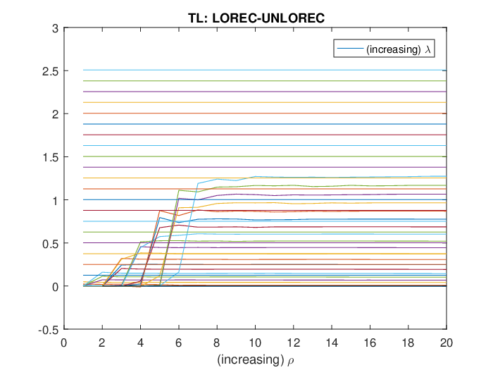
We start analyzing the performance of in comparison to the one of on our reference setting (Setting 1). In Figure 8 and 9 we report the differences between the Sample Total Losses and the Total Losses of LOREC and UNALCE for a grid of threshold pairs. We note that the gain is positive everywhere, with the exception of the threshold pairs which do not return the exact rank (because they do not satisfy the range of Theorem 2.1). This pattern is more remarkable for Sample Total Loss than for Total Loss. For both losses and each , we note that, as explained, the gain across never overcomes its maximum (plotted for each ).

In Figure 10 we report the plot of the estimated proportion of latent variance across thresholds for (in solid line the true ). In Figure 11 the same plot is reported for . The shape is exactly the same as for , the only difference is that all patterns are negatively shifted. In particular, gets closer to for respect to in correspondence to all threshold combinations.


Setting 1 Setting 2 Setting 3 UNALCE POET UNALCE POET UNALCE POET 0.6952 0.7314 0.6955 0.7324 0.7987 0.8151 0.0034 0.0000 0.0071 0.0000 0.0035 0.0000 0.0299 0.0003 0.0915 0.0079 0.1287 0.0132 6.98 7.39 11.69 11.70 9.95 10.47 0.72 2.79 0.57 2.22 1.26 3.85 7.63 9.32 12.36 12.95 11.39 13.26 6.91 7.58 11.59 11.62 9.85 10.74 0.72 1.74 0.78 1.33 1.55 2.52
Setting 2 Setting 4 Setting 5 UNALCE POET UNALCE POET UNALCE POET 0.6955 0.7324 0.7980 0.8233 0.7932 0.8284 0.0071 0.0000 0.0022 0.0000 0.0004 0.0000 0.0915 0.0079 0.0164 0.0115 0.0015 0.0010 11.69 11.70 13.02 13.31 20.92 21.41 0.57 2.22 1.94 2.90 3.91 4.38 12.36 12.95 14.25 14.89 22.49 23.97 11.59 11.62 12.93 13.38 20.85 21.53 0.78 1.33 1.32 1.51 1.65 2.44
Setting 1 Setting 2 Setting 3 UNALCE POET UNALCE POET UNALCE POET 0.0195 0.0242 0.0967 0.1250 0.0626 0.0808 0.111 0.0000 0.0183 0.0001 0.0193 0.0003 0.0093 0.0238 0.0507 0.1172 0.0270 0.0676 0.7019 0.0000 0.6977 0.0002 0.6077 0.0010 0.7105 0.0000 0.6909 0.0000 0.6294 0.0000 0.9869 0.9997 0.9536 0.9911 0.9387 0.9859
Setting 2 Setting 4 Setting 5 UNALCE POET UNALCE POET UNALCE POET 0.0967 0.1250 0.0321 0.0435 0.0359 0.0375 0.0183 0.0001 0.0147 0.0001 0.0025 0.0000 0.0507 0.1172 0.0245 0.0320 0.0356 0.0366 0.6977 0.0002 0.2318 0.0001 0.0284 0.0000 0.6909 0.0000 0.2414 0.0000 0.0262 0.0000 0.9536 0.9911 0.9915 0.9882 0.9995 0.9990
Setting 1 Setting 2 Setting 3 UNALCE POET UNALCE POET UNALCE POET 5.50 5.74 11.14 11.62 5.64 6.07 0.29 1.55 0.26 1.17 0.43 1.86 7.75 7.16 14.52 15.24 5.65 6.16 104110 34048 114210 14452 2207400 1141400 21571 4776.3 65628 1310.2 125170 40407 1.32 1.32 1.54 1.55 4.07 3.97 20.84 21.84 21.90 22.59 130.22 131.58 3.77 2.75 2.66 1.90 5.67 4.15 19.84 21.00 21.00 22.01 128.50 130.39
Setting 2 Setting 4 Setting 5 UNALCE POET UNALCE POET UNALCE POET 11.14 11.62 6.06 6.24 10.06 10.57 0.26 1.17 0.49 1.15 0.81 1.92 14.52 15.24 6.07 6.34 10.43 10.57 114210 14452 28321 192790 12857 20171 65628 1310.2 2469 1132.2 1406.9 1430 1.54 1.55 2.41 2.35 2.99 2.85 21.90 22.59 35.34 36.03 42.48 43.57 2.66 1.90 2.73 1.90 4.49 3.15 21.00 22.01 35.68 34.88 43.17 42.00
Table 6 contains some results about fitting measures across different degrees of spikiness (Settings 1,2,3). It is clear that UNALCE outperforms POET concerning all losses, and shows the superior performance of UNALCE concerning the proportion of latent variance, of residual covariance, of detected non-zeros. The same pattern can be deduced from Table 7, which contains the same results across different ratios (Settings 2,4,5). Nevertheless, we note that the gap progressively decreases as increases, due to the increased consistency with POET assumptions. We note, for instance, that the proportion of residual covariance is underestimated also by UNALCE for . At the same time, the performance of the proportion of residual variance detected by POET is upper biased, due to the natural bias of sample eigenvalues, and the bias decreases as the degree of spikiness increases.
Tables 8 and 9 contain the error measures about the detection of the residual pattern across the degree of spikiness and the ratio respectively. We note that POET, due to the lack of algebraic consistency, is completely unable to classify positive and negative elements. On the contrary, UNALCE shows a recovery rate around when is small, while the detection capability deteriorates as increases.
Tables 10 and 11 report the Euclidean distance between the vectors of estimated and true eigenvalues (denoted by ), the condition number of the estimates and the estimated spectral norms. This Table can be compared to Table 4 which contains the true spectral norms and condition numbers across settings. All statistics are generally in favour of UNALCE with some notable exceptions motivated by our theory. If is low and the eigenvalues are not spiked, the spectral norm tend to be underestimated by UNALCE, because the eigenvalues tend to be smaller and more concentrated. On the contrary, UNALCE may overestimate the condition number of and if is large, because the guarantee required for positive definiteness is stronger.
To sum up, our UNALCE estimator outperforms POET concerning fitting and conditioning properties, detection of sparsity pattern, and eigen-structure recovery. We note that POET does not detect positive and negative elements at all. This is because it only has parametric consistency and not also the algebraic one. In addition, in order to obtain a positive definite estimate, cross validation selects a very high threshold for POET, and this causes the sparse estimate to be almost completely diagonal if is large. On the contrary, the mathematical optimization procedure of UNALCE gets closer to the target and ensures to catch the algebraic spaces behind the two components.
Appendix B Proofs
B.1 Proof of Theorem 2.1
Theorem 2.1 relies on proving the equivalent of the following Lemma by Fan et al. (2013)
Lemma B.1
| (40) |
under our assumption setting. Lemma (40) in turn relies on the following Lemmas by Fan et al. (2011):
Lemma B.2
Lemma B.3
Lemma B.4
The first step of the proof consists in decomposing in its four components:
where:
where and are respectively the vectors of factor scores and residuals for each observation.
From the inequality (Fan et al. (2008), page 194, Assumption (B)), Lemma B.2 follows under Assumption 2.3. Therefore, Lemma B.2 is unaffected. Consequently, following Fan et al. (2013), we can argue that
In order to show how Lemma B.3 changes, we need to recall some key results of Bickel and Levina (2008a). Differently from Luo’s approach, in that setting (as in ours and in the POET one) the sparsity assumption is imposed to , and not to . While in Fan et al. (2013) the assumption , is needed to ensure POET consistency, here Assumption 2.4 prescribes .
Consider now the uniformity class of sparse matrices in Bickel and Levina (2008a) (with ):
| (41) |
Under Assumption 2.4 this class is no longer appropriate, because we can no longer write (see Bickel and Levina (2008a), page 2580)
since the quantity no longer scales to but to . Therefore, we need to replace by in the proof which derives the rate of the sample covariance matrix under class (41) (see Bickel and Levina (2008a), page 2582), thus proving under Assumptions 2.3 and 2.4 that:
Lemma B.5
To conclude, we analyze Lemma B.4:
Exploiting Assumption 2.5 we obtain . Therefore, the bound above becomes .
Applying the recalled proof strategy to we obtain
because by Assumption 2.1. The condition finally leads to:
| (43) |
Therefore, the following bound is proved
| (44) |
because from Assumption 2.2. In fact, if the condition of Theorem 2.1 would result in , thus violating Assumption 2.1.
In other words, the bound (44) means
| (45) |
The proof relies on the combined use of proof tools by Fan et al. (2013), Fan et al. (2011), Fan et al. (2008) and Bickel and Levina (2008a).
Exploiting the basic property and the minimum for in the range of Theorem 2.1, we can simply write
| (46) |
According to Chandrasekaran et al. (2012) and Luo (2011a), the only probabilistic component of the error norm is . Therefore, following the proof of Luo (2011a) and setting , we can finally prove, under all the assumptions and conditions of Theorem 2.1, the thesis
| (47) |
B.2 Proof of Corollary 2.1
The proof directly descends by bound (44), because if and only if as . As expected, the absolute bound vanishes only in the small dimensional case ().
B.3 Proof of Corollary 2.2
Defined as the covariance matrix formed by the first principal components, we know by dual Lidskii inequality that
We start studying the behaviour of . From bound (44) it descends the following Lemma
Lemma B.6
Let be the th largest eigenvalue of . If , then with probability approaching for some .
By Lidskii dual inequality, in fact, we note
Applying Lidskii dual inequality to we have . If , we obtain by Assumption 2.1, which means that is bounded away from and as we divide by for . Otherwise, we obtain .
Applying Weyl’s inequality to we obtain by bound (44). Therefore, dividing by , .
Finally, assuming , vanishes asymptotically dividing by because both the relative errors of and vanish (once assumed that is known a priori or consistently estimated by UNALCE).
Then Corollary 2.2 is proved because .
B.4 Proof of Theorem 2.2
Conditioning on , and , we aim to solve
By Cauchy-Schwartz inequality, it can be shown that
solves the problem
conditioning on the fact that is minimum over the same set.
Then we can write
By Cauchy-Schwartz inequality, it can be shown that
Hence
| (48) |
The problem in is solved taking out the first principal components of . By construction, the solution is .
The problem in , assuming that the diagonal of is given and the off-diagonal elements of are invariant, leads to:
The question now becomes: which diagonal elements of ensure the minimum of ? Term is fixed respect to , because we are assuming the invariance of diagonal elements in (). The minimization of term , given that , falls back into the previous case, i.e. is minimum if and only if .
Optimality holds over the cartesian product of the set of all positive semi-definite matrices with rank smaller or equal to , , and the set of all sparse matrices with the same sparsity pattern as such that , (we call this set .
Consequently, we can write:
B.5 Proof of Corollary 2.3
We know that . We can prove that
conditioning on the event
under prescribed assumptions (see Theorem 2.2). In fact we can write
because is uniquely determined by the conditioning event. The same inequality holds in spectral norm.
Since it holds
we can write
| (49) |
given the conditioning event. As a consequence, since , we obtain
| (50) |
The analogous triangular inequality for the sparse component is
In order to quantify , we need to study the behaviour of the term , which is less or equal to , because it is less or equal to .
As a consequence, we have . Analogously to , we can prove that
conditioning on the event
under prescribed assumptions (see Theorem 2.2). In fact we can write
because is uniquely determined by the conditioning event.
Therefore, we can write
| (51) |
The claim on is less immediate. We recall that . can be divided in the contribution coming from diagonal elements and the rest: . Both contributes are part of .
Given the matrix of eigenvectors , we can write , where is a null matrix except for the -th diagonal element equal to and is the -th row of . Similarly we can write where is a null matrix except for the element equal to . Note that the rows of , differently from the columns, are not orthogonal.
Since all summands are orthogonal to each other (), the triangular inequalities relative to , and become equalities. Therefore we can write:
| (52) | |||
| (53) | |||
| (54) |
From this consideration it follows that
Since, by definition, (because ), and recalling that has the best approximation property (for Theorem 2.2) given the conditioning event, we can conclude
| (55) |
B.6 Proof of Corollary 2.4
The relevant triangular inequality for the overall estimate is
We know that, by definition, . For the same considerations explained before,
As a consequence, recalling that under the described assumptions, we can conclude
| (56) |
Since , we have
| (57) |
We can then claim
| (58) |
Therefore, the real gain is terms of approximation of respect to ALCE measured in squared Frobenius norm is strictly positive and bounded from .
B.7 Proof of Theorem 2.3
Conditioning on , we can easily write
| (59) |
The quality of the estimation input does not depend on the estimation method.
Analogously, it is easy to prove that
| (61) |
B.8 Proof of Corollary 2.5
We recall the following expression:
From (61) we can conclude that
| (62) |
Analogously, since it holds
it is straightforward that
| (63) |
B.9 Proof of Corollary 2.6
We prove in sequence the three claims of the Corollary.
- 1.
We start noting that , and are - ranked. We denote the respective spectral decompositions by:
- (a)
with ;
- (b)
with ;
- (c)
As a consequence, by Lidskii dual inequality we note that
which proves the claim on .
- (a)
- 2.
By Lidskii dual inequality, we note that
The matrix is a -dimensional squared matrix having as th element the quantity , where , , is the i-th row of the matrix . Since , it descends that
, i.e.Therefore we obtain
which proves the claim on .
- 3.
By Lidskii dual inequality, we note that
Recalling the argument above and noting that
because , it descendswhich proves the claim on .
References
- Agarwal et al. (2012) Agarwal, A., S. Negahban, and M. J. Wainwright (2012). Noisy matrix decomposition via convex relaxation: Optimal rates in high dimensions. The Annals of Statistics, 1171–1197.
- Anderson (1984) Anderson, T. (1984). Multivariate statistical analysis. Wiley and Sons, New York, NY.
- Bai (2003) Bai, J. (2003). Inferential theory for factor models of large dimensions. Econometrica 71(1), 135–171.
- Bai and Ng (2002) Bai, J. and S. Ng (2002). Determining the number of factors in approximate factor models. Econometrica 70(1), 191–221.
- Bickel and Levina (2008a) Bickel, P. J. and E. Levina (2008a). Covariance regularization by thresholding. The Annals of Statistics, 2577–2604.
- Bickel and Levina (2008b) Bickel, P. J. and E. Levina (2008b). Regularized estimation of large covariance matrices. The Annals of Statistics, 199–227.
- Cai et al. (2010) Cai, J.-F., E. J. Candès, and Z. Shen (2010). A singular value thresholding algorithm for matrix completion. SIAM Journal on Optimization 20(4), 1956–1982.
- Cai and Liu (2011) Cai, T. and W. Liu (2011). Adaptive thresholding for sparse covariance matrix estimation. Journal of the American Statistical Association 106(494), 672–684.
- Cai et al. (2010) Cai, T. T., C.-H. Zhang, and H. H. Zhou (2010, 08). Optimal rates of convergence for covariance matrix estimation. The Annals of Statistics 38(4), 2118–2144.
- Chandrasekaran et al. (2012) Chandrasekaran, V., P. A. Parrilo, and A. S. Willsky (2012, 08). Latent variable graphical model selection via convex optimization. The Annals of Statistics 40(4), 1935–1967.
- Chandrasekaran et al. (2011) Chandrasekaran, V., S. Sanghavi, P. A. Parrilo, and A. S. Willsky (2011). Rank-sparsity incoherence for matrix decomposition. SIAM Journal on Optimization 21(2), 572–596.
- Clarke (1990) Clarke, F. H. (1990). Optimization and nonsmooth analysis. SIAM.
- Daubechies et al. (2004) Daubechies, I., M. Defrise, and C. De Mol (2004). An iterative thresholding algorithm for linear inverse problems with a sparsity constraint. Communications on pure and applied mathematics 57(11), 1413–1457.
- Davidson and Szarek (2001) Davidson, K. R. and S. J. Szarek (2001). Local operator theory, random matrices and banach spaces. Handbook of the geometry of Banach spaces 1(317-366), 131.
- Dey and Srinivasan (1985) Dey, D. K. and C. Srinivasan (1985). Estimation of a covariance matrix under stein’s loss. The Annals of Statistics, 1581–1591.
- Fan et al. (2008) Fan, J., Y. Fan, and J. Lv (2008). High dimensional covariance matrix estimation using a factor model. Journal of Econometrics 147(1), 186–197.
- Fan et al. (2016) Fan, J., Y. Liao, and H. Liu (2016). An overview of the estimation of large covariance and precision matrices. The Econometrics Journal 19(1).
- Fan et al. (2011) Fan, J., Y. Liao, and M. Mincheva (2011). High dimensional covariance matrix estimation in approximate factor models. The Annals of Statistics 39(6), 3320–3356.
- Fan et al. (2013) Fan, J., Y. Liao, and M. Mincheva (2013). Large covariance estimation by thresholding principal orthogonal complements. Journal of the Royal Statistical Society: Series B (Statistical Methodology) 75(4), 603–680.
- Farné (2016) Farné, M. (2016). Large Covariance Matrix Estimation by Composite Minimization. Ph. D. thesis, Alma Mater Studiorum.
- Farné and Montanari (2018) Farné, M. and A. Montanari (2018). A large covariance matrix estimator under intermediate spikiness regimes. https://data.mendeley.com/datasets/nh97vfvhkt.
- Fazel (2002) Fazel, M. (2002). Matrix rank minimization with applications. Ph. D. thesis, PhD thesis, Stanford University.
- Fazel et al. (2001) Fazel, M., H. Hindi, and S. P. Boyd (2001). A rank minimization heuristic with application to minimum order system approximation. In American Control Conference, 2001. Proceedings of the 2001, Volume 6, pp. 4734–4739. IEEE.
- Friedman et al. (2008) Friedman, J., T. Hastie, and R. Tibshirani (2008). Sparse inverse covariance estimation with the graphical lasso. Biostatistics 9(3), 432–441.
- Furrer and Bengtsson (2007) Furrer, R. and T. Bengtsson (2007). Estimation of high-dimensional prior and posterior covariance matrices in kalman filter variants. Journal of Multivariate Analysis 98(2), 227–255.
- Lam et al. (2016) Lam, C. et al. (2016). Nonparametric eigenvalue-regularized precision or covariance matrix estimator. The Annals of Statistics 44(3), 928–953.
- Ledoit and Wolf (2004) Ledoit, O. and M. Wolf (2004). A well-conditioned estimator for large-dimensional covariance matrices. Journal of multivariate analysis 88(2), 365–411.
- Ledoit and Wolf (2015) Ledoit, O. and M. Wolf (2015). Spectrum estimation: A unified framework for covariance matrix estimation and pca in large dimensions. Journal of Multivariate Analysis 139, 360–384.
- Luo (2011a) Luo, X. (2011a). High dimensional low rank and sparse covariance matrix estimation via convex minimization. Arxiv preprint.
- Luo (2011b) Luo, X. (2011b). Recovering model structures from large low rank and sparse covariance matrix estimation. arXiv preprint arXiv:1111.1133.
- Nesterov (2013) Nesterov, Y. (2013). Gradient methods for minimizing composite functions. Mathematical Programming 140(1), 125–161.
- Qiu and Chen (2015) Qiu, Y. and S. X. Chen (2015). Bandwidth selection for high-dimensional covariance matrix estimation. Journal of the American Statistical Association 110(511), 1160–1174.
- Rockafellar (2015) Rockafellar, R. T. (2015). Convex analysis. Princeton university press.
- Rothman et al. (2009) Rothman, A. J., E. Levina, and J. Zhu (2009). Generalized thresholding of large covariance matrices. Journal of the American Statistical Association 104(485), 177–186.