Ultra-Red Galaxies Signpost Candidate Proto-Clusters at High RedshiftNote: To be submitted to The Astrophysical Journal
Abstract
We present images obtained with the Atacama Pathfinder Experiment (APEX) telescope’s Large APEX BOlometer CAmera (LABOCA) of a sample of 22 galaxies selected via their red Herschel SPIRE (Spectral and Photometric Imaging Receiver) 250-, 350- and - colors. We aim to see if these luminous, rare and distant galaxies are signposting dense regions in the early Universe. Our survey covers an area of down to an average r.m.s. of , with our five deepest maps going deeper still. We catalog 86 dusty star-forming galaxies (DSFGs) around our ‘signposts’, detected above a significance of . This implies a over-density of DSFGs, excluding our signposts, when comparing our number counts to those in ‘blank fields’. Thus, we are 99.93% confident that our signposts are pinpointing over-dense regions in the Universe, and % [50%] confident that these regions are over-dense by a factor of at least []. Using template spectral energy distributions and SPIRE/LABOCA photometry we derive a median photometric redshift of for our signposts, with an interquartile range of , somewhat higher than expected for -selected galaxies. We constrain the DSFGs likely responsible for this over-density to within of their respective signposts; over half of our ultra-red targets () have an average of two DSFGs within . These ‘associated’ DSFGs are radially distributed within (physical) distances of from their signposts, have median star-formation rates (SFRs) of (for a Salpeter stellar initial mass function) and median gas reservoirs of . These candidate proto-clusters have average total SFRs of at least and space densities of , consistent with the idea that their constituents may evolve to become massive early-type galaxies in the centers of the rich galaxy clusters we see today.
Subject headings
galaxies: clusters: general — galaxies: high-redshift — galaxies: starburst — infrared: galaxies — submillimeter: galaxiesI. Introduction
Galaxy clusters whose cores are rich with early-type galaxies (ETGs, i.e. relatively passive ellipticals and lenticulars) mark the densest regions in the distribution of dark matter (DM), regions which have grown hierarchically from initial, Gaussian fluctuations, supposedly etched into the Universe at some arbitrarily early epoch [76, 115, 95, e.g.]. In the local Universe, these galaxy clusters harbor the majority of ETGs, which in turn harbor over half of the present-day stellar mass (). Thus studying their cosmic evolution can place valuable constraints on models of galaxy formation [96, 82, 74, 57, e.g.].
ETGs obey a tight scaling relation between their color and magnitude, where magnitude equates roughly to . This is known as the ‘red sequence’, in which more massive galaxies are typically redder with older stellar populations and less ongoing star formation [13, 4, 12, 7, e.g.]. Furthermore, ETGs in local galaxy clusters appear redder (and thus more massive, since they follow the scaling relation) as their distance to the cluster center decreases [9]. These properties are consistent with the concept of ‘cosmic downsizing’ (Cowie et al., 1996; and see Fig. 9 in Thomas et al., 2010), whereby the most massive ETGs formed their stars early () and over relatively short timescales [68, 106, 107, 94, 104, 105, —].
ETGs have commonly been viewed as transformed late-type galaxies (LTGs, i.e. star-forming spirals) which have had their star formation quenched via some mechanism, leaving behind an ETG on the red sequence [33, 41]. In local galaxy clusters this quenching is brought about rapidly via ram pressure stripping [46] or by so-called ‘starvation’ and/or ‘strangulation’ processes11 1 Galaxy clusters reside in deep gravitational potentials which heat the intracluster medium (ICM). As a consequence, the ICM strips the cold gas from infalling LTGs and subsequently starves/strangles them of cold gas, the fuel for further star formation. [59, 5, 35, 26, 104, 16]. However, at higher redshifts, could the most-massive ETGs, in the centers of galaxy clusters, be the remnants of colossal merger events instead?
An extreme event like this would require wildly different behavior for the precursors of ETGs at , with such systems exhibiting immensely high star-formation rates (SFRs, ). In a hierarchical context this large burst of star formation is driven by mergers in dense environments [56]. Although the existence of such large systems at such high redshifts places stress on the hierarchical paradigm [43], it is conceivable that dusty star-forming galaxies [10, 18, DSFGs — e.g.] are associated with these distant events at an epoch when the merger rates are comparatively high [47, 31].
Conventional wisdom places this dusty population at [21, 92], but recent work by Riechers et al. [79], Dowell et al. [32], Asboth et al. [2] and Ivison et al. [52, hereafter Paper I ], to name but a few, suggests that a rare, subset can be identified via their red, far-infrared (far-IR) colors as measured by the Spectral and Photometric Imaging Receiver [45, SPIRE —] on board the Herschel Space Observatory [77]. Lensed DSFGs at similarly high redshifts have also been found by surveys at with the South Pole Telescope – relying on flux-density ratios at even longer wavelengths to generate a sample of distant, dust-dominated sources [111, 114, 100].
With remarkably high median rest-frame, luminosities, , these so-called ‘ultra-red galaxies’ can provide the SFRs necessary to give birth to the most-massive ETGs in the centers of galaxy clusters and, thus, the red sequence. In this work, we go one step further than 52 exploiting a representative sample of ultra-red galaxies to decipher whether these DSFGs exhibit evidence of clustering consistent with their eventual membership of massive galaxy clusters at .
If ultra-red galaxies do indeed trace the precursors of the most massive ETGs in the centers of present-day galaxy clusters, we would expect to witness comparatively22 2 This important semantic reflects the fact that on some scale any system could be virialized, for e.g., a single proto-cluster may be unvirialized (for some foreseeable dynamical time) but it is comprised of many tens of virialized components. unvirialized systems characterized by over-densities of (physically associated) DSFGs [65, 17, i.e. a ‘proto-cluster’ —]. Such systems have already been discovered in the Universe via their submillimeter (submm) emission, with previous work typically relying either on high-redshift radio galaxies [49, 99, 98, 81, HzRGs — e.g.], pairs of quasi-stellar objects [109, QSOs —] or even strong over-densities of Lyman- emitters as signposts [15, 103, 108]. Predictions by Negrello et al. [66] suggested that bright-intensity peaks within low-resolution data taken with the Planck High Frequency Instrument, could represent of clumps DSFGs. Indeed, over-densities of DSFGs at have been found using this technique [23, i.e. ‘HATLAS12-00’ —].
Although DSFGs appear to be poor tracers of large structure below [63], the situation appears to be quite different by [62, 72] – albeit care must be taken when discovering over-densities within a rare (thus low-numbered) population of galaxy. At odds with this concept is the most-distant (), ultra-red galaxy discovered to date, ‘HFLS 3’ [79]. Confusion-limited observations of the environments surrounding this DSFG showed little evidence that it signposted an over-density of DSFGs [83]. However, in light of new and improved comparison data, it appears that HFLS 3 perhaps signposts regions that are over-dense by a factor of at least .
Thus, if our sample of ultra-red galaxies shows an excess of DSFGs compared to the field then we will have confirmed this novel technique for pinpointing primordial over-densities in the distant Universe. Combined with follow-up optical imaging/spectroscopy of their environments [97, 60, to detect so-called ‘Lyman-break’ galaxies, LBGs —] , we will be able to place strong constraints on their and DM components. A joint approach – combining models [96, e.g.] and observations – is necessary to fully predict the eventual fate of these proto-clusters at [17, 73] .
The structure of this paper is as follows. In the next section we outline our target sample, as well as our data acquisition and reduction methods. We analyze our data in §III and discuss their implications in §IV. Finally, our conclusions are presented in §V. Throughout our analysis and discussion, we adopt a ‘concordance cosmology’ with , and [48], in which corresponds to a (proper) distance of at . For a quantity, , we denote its mean and median values as and , respectively.
II. Target Sample and Data reduction
II.1. Target sample
We selected 12 targets33 3 These targets were initially chosen for follow-up observations as their preliminary, albeit shallow, data at suggested that they were robust detections. from the H-ATLAS [34, Herschel Astrophysical Terahertz Large Area Survey —] imaging survey. These targets are contained in the Data Release 1 [110, 11, dr1 —] H-ATLAS images of the two equatorial Galaxy And Mass Assembly (GAMA 09 and GAMA 15) fields and the South Galactic Pole (SGP) field. Our selection criteria are discussed fully in 52, which we briefly outline here.
We imposed color cuts of and in order to select rare, distant galaxies. We increased the reliability of our ultra-red galaxy sample by imposing a significance of , and by requiring flux densities consistent with a high redshift in ground-based snapshot images obtained at 850 or .
Additionally, we required that in order to reduce the fraction of gravitationally lensed galaxies in favour of intrinsically luminous galaxies [67, 25], though we draw attention to SGP-28124, with a flux density , which is significantly higher than its cataloged flux density at the time of our observations.
To this H-ATLAS sample, we added an additional ten targets from five fields in the HerMES [70, Herschel Multi-tiered Extragalactic Survey —] imaging survey – ultra-red galaxies selected in the Akari Deep Field-South (ADF-S), the Chandra Deep Field-South Survey (CDFS), the European Large-Area Infrared Survey-South 1 (ELAIS-S1) and the XMM/Newton-Large-Scale Survery fields are contained in the dr4.0 xID250 catalogs by Roseboom et al. [86], Roseboom et al. [87], whilst those selected from the HerMES Large Mode Survey (HeLMS) are amongst the 477 red galaxies presented by Asboth et al. [2]. All HerMES images and catalogs were accessed through the Herschel Database in Marseille [84, HeDaM —]44 4 http://hedam.oamp.fr/hermes/..
II.2. Observing strategy
| Nickname | (J2000) | Date observed | Program | |||||
|---|---|---|---|---|---|---|---|---|
| hr | yyyy–mm | |||||||
| SGP-28124 | 00:01:24.73 | 35:42:13.7 | 13.4 | 0.3 | 1.9 | 133 | 2013–04 | E-191.A-0748 |
| HeLMS-42 | 00:03:04.39 | 02:40:49.8 | 0.8 | 0.3 | 6.3 | 121 | 2013–10 | M-092.F |
| SGP-93302 | 00:06:24.26 | 32:30:21.4 | 16.6 | 0.3 | 1.7 | 129 | 2013–04 | E-191.A-0748 |
| ELAIS-S1-18 | 00:28:51.23 | 43:13:51.5 | 0.9 | 0.2 | 5.3 | 117 | 2013–04 | M-091.F |
| ELAIS-S1-26 | 00:33:52.52 | 45:20:11.9 | 4.4 | 0.4 | 4.0 | 118 | 2014–04 | M-093.F |
| SGP-208073 | 00:35:33.82 | 28:03:03.2 | 4.9 | 0.3 | 3.2 | 130 | 2013–04 | M-091.F, E-191.A-0748, M-092.F |
| ELAIS-S1-29 | 00:37:56.76 | 42:15:20.5 | 2.9 | 0.3 | 4.2 | 137 | 2013–10 | M-092.F, M-093.F |
| SGP-354388 | 00:42:23.23 | 33:43:41.8 | 11.4 | 0.3 | 1.8 | 124 | 2013–10 | M-092.F, E-191.A-0748 |
| SGP-380990 | 00:46:14.80 | 32:18:26.5 | 4.0 | 0.3 | 2.9 | 115 | 2012–11 | M-090.F |
| HeLMS-10 | 00:52:58.61 | 06:13:19.7 | 0.5 | 0.3 | 8.0 | 114 | 2013–10 | M-092.F |
| SGP-221606 | 01:19:18.98 | 29:45:14.4 | 1.3 | 0.4 | 6.0 | 112 | 2014–05 | M-093.F |
| SGP-146631 | 01:32:04.35 | 31:12:34.6 | 2.4 | 0.3 | 5.0 | 119 | 2014–04 | M-093.F |
| SGP-278539 | 01:42:09.08 | 32:34:23.0 | 3.2 | 0.4 | 4.4 | 121 | 2014–04 | M-093.F |
| SGP-142679 | 01:44:56.46 | 28:41:38.3 | 3.0 | 0.4 | 4.3 | 116 | 2014–04 | M-093.F |
| XMM-LSS-15 | 02:17:43.86 | 03:09:11.2 | 2.0 | 0.3 | 4.4 | 118 | 2013–10 | M-092.F |
| XMM-LSS-30 | 02:26:56.52 | 03:27:05.0 | 4.1 | 0.3 | 3.4 | 132 | 2013–09 | E-191.A-0748, M-090.F, M-092.F |
| CDFS-13 | 03:37:00.91 | 29:21:43.6 | 1.0 | 0.2 | 5.3 | 118 | 2013–10 | M-092.F |
| ADF-S-27 | 04:36:56.47 | 54:38:14.6 | 3.4 | 0.3 | 3.7 | 135 | 2012–09 | M-090.F |
| ADF-S-32 | 04:44:10.30 | 53:49:31.4 | 2.0 | 0.3 | 5.0 | 129 | 2013–04 | M-091.F, M-092.F |
| G09-83808 | 09:00:45.41 | 00:41:26.0 | 9.2 | 0.3 | 1.8 | 125 | 2013–10 | E-191.A-0748 |
| G15-82684 | 14:50:12.91 | 01:48:15.0 | 6.7 | 0.3 | 2.3 | 116 | 2014–03 | M-093.F |
| SGP-433089 | 22:27:36.98 | 33:38:33.9 | 13.2 | 0.3 | 1.8 | 117 | 2012–09 | M-090.F, M-091.F, M-093.F |
† Average depth computed across each beam-smoothed LABOCA map, where the resulting FWHM of a beam is .
‡ Extent of LABOCA map.
Note. Targets are listed in order of increasing right ascension.
Our sample of 22 ultra-red galaxies were imaged with the Atacama Pathfinder Experiment (APEX) telescope’s Large APEX BOlometer CAmera [55, 93, LABOCA —] instrument over six observing runs from 2012 September to 2014 March55 5 ESO program E-191.A-0748 and MPI programs M-090.F-0025-2012, M-091.F-0021-2013 and M-092.F-0015-2013.. The passband response for this instrument is centered on () and has a half-transmission width of ().
Targets were observed in a compact-raster scanning mode, whereby the telescope scans in an Archimedean spiral for at four equally spaced raster positions in a grid. Each scan was approximately long such that each raster position was visited three times, leading to a fully sampled map over the full -diameter field of view of LABOCA. An average time of was spent integrating on each target. Maps with longer integration times () provide deeper data sensitive to less luminous DSFGs in the vicinity of our signposts. Our shallower maps () help constrain the abundances of the brightest DSFGs, thus reducing the Poisson noise associated with these rare galaxies. These deep/shallow data are necessary to constrain the photometric redshifts of the brighter/fainter DSFGs within the vicinities of our signposts, therefore allowing us to identify members of any candidate proto-cluster found.
During our observations, we recorded typical precipitable water vapor (PWV) values between , corresponding to a zenith atmospheric opacity of . Finally, the flux density scale was determined to an r.m.s. accuracy of using observations of primary calibrators, Uranus and Neptune, whilst pointing was checked every hour using nearby quasars and found to be stable to (r.m.s.).
II.3. From raw timestreams to maps
The data were reduced using the Python-based BOlometer data Analysis Software package [88, BOA v4.1 —], following the prescription outlined in §10.2 and §3.1 of Siringo et al. [93] and Schuller et al. [89], respectively. We briefly outline the reduction steps below.
- –
Timestreams for each scan were calibrated onto the scale using primary or secondary flux density calibrators.
- –
Channels exhibiting strong cross talk with their neighbors, showing no signal or high noise were flagged, whilst the remaining channels were flatfielded.
- –
Timestreams were flagged in regions where the speed and acceleration of the telescope are too severe to guarantee reliable positional information at every timestamp.
- –
In an iterative manner, the following sequence was performed:
- 1.
Noisy channels were -clipped relative to all channels, where with each iteration.
- 2.
Sky noise determined across all channels was removed from each channel.
- 3.
Each channel’s timestreams were ‘despiked’ about their mean value.
- 4.
An -order polynomial baseline was subtracted from the timestreams to remove any low frequency drifts, where with each iteration.
- 1.
- –
Large discontinuities (jumps) in the timestreams, seen by all channels, and correlated noise between groups of channels (e.g. channels sharing the same part of the electronics or being connected to the same cable) were removed.
- –
The Fourier spectrum of the timestreams were high-pass filtered below using a noise-whitening algorithm to remove the noise. At this stage, the mean noise-weighted point-source sensitivity of all channels was calculated to remove scans corrupted by electronic interference. Uncorrupted scans were opacity-corrected using skydips and radiometer opacity values before being pixelated onto a map. We over-sampled the pixelization process by a factor of four to preserve the spatial information in the map. This results in a final map for a given scan with a pixel scale, .
We coadded, with inverse weighting, all of the reduced maps for each scan before beam smoothing the final map to remove any high-frequency noise on scales smaller than the beam. The effect of convolving with a Gaussian with full-width-at-half-maximum (i.e. the beam width, see Fig. 1) degrades the spatial resolution to . Thus we appropriately scale the final map in order to preserve the peak intensity.
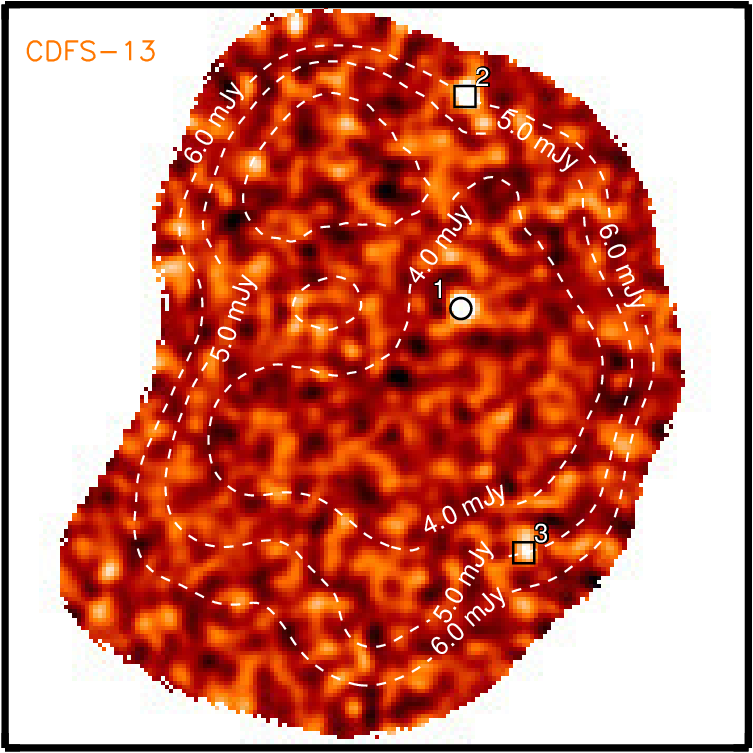
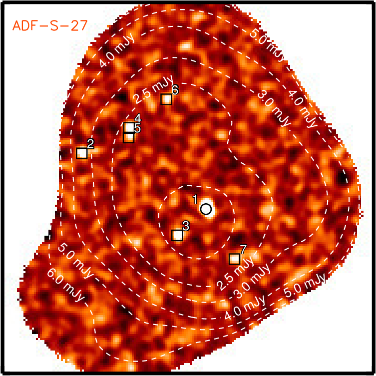
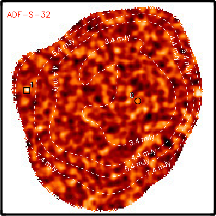
We repeated these reduction steps, this time using the final reduced map as a model to mask significant sources before flagging the timestreams. Using a model in this fashion helps to increase the final signal-to-noise ratio () of detections [89, 69, 8]. We find that one repetition is sufficient to achieve convergence in the of a point source, in agreement with the findings of Weiß et al. [113] and Gomez et al. [42]. We present the final maps for all of our ultra-red galaxies in Appendix A.

To model the instrumental noise of our maps, we generated so-called ‘jackknife’ maps by randomly inverting (i.e. multiplying by ) half of our reduced scans before coadding them. The result is a map free of astronomical sources and confusion, which we estimate to be in our deepest maps, and thus these realizations will underestimate the true noise. For each map, we created 100 jackknife realizations of the instrumental noise.
In Fig. 2, we show the pixel distributions of the final maps and their respective jackknife realizations. There is clearly a positive excess above in the final reduced maps compared to the jackknife maps. This excess is caused by the presence of astronomical sources.
III. Analysis


We chose a detection threshold () based on the values of a ‘fidelity’ or ‘trustworthiness’ parameter, , similar to that outlined in Aravena et al. [1]. For all of our maps, we ran our extraction algorithm (§III.1) and compared the number of sources detected in our maps, , to the mean number of sources detected in our 100 jackknife realizations for each map, , as a function of detection :
| (1) |
We show the average fidelity in the right-hand panel of Fig. 2 which illustrates that by increasing the detection we increase our confidence in the recovered sources. We reach a fidelity of at and a fidelity of at , the latter indicating that we would expect about half of our sources to be spurious at . We chose – as a compromise between reliability and the number of cataloged sources – a detection threshold of , where we have a fidelity, .
The intrinsic map-to-map scatter in the fidelity is caused by the varying abundance of sources in each map, due to the effects of cosmic variance and the differing r.m.s. noise levels. This scatter decreases with increasing detection threshold and is at .
III.1. Source extraction
We used a custom-written Interactive Data Language [58, idl —] source extraction algorithm to identify and extract sources in the beam-smoothed maps, noting that the beam-smoothing step described above optimizes the detection of point sources.
In a top-down fashion, we searched for pixels above66 6 To accommodate sources whose true peak falls between pixels we temporarily lowered by , keeping sources with bicubically interpolated sub-pixel values that meet our original detection threshold. our floor detection threshold . In Table 4, we catalog the peak flux density, noise and position determined from a three-parameter Gaussian fit made inside a box of width (i.e. ) centered on a source. After removing the fit from the map, we searched for and cataloged subsequent peaks until no more could be found.
During the extraction process we performed some additional steps: sources deemed too close to each other () have their parameters re-evaluated, fitting multiple three-parameter Gaussians simultaneously; sources deemed too close () to the map edges were rejected.
III.1.1 Completeness, flux boosting and positional offsets
We inserted simulated sources into our jackknife maps to quantify the statistical properties of our cataloged sources. To ensure that we did not encode any clustering, we randomize the injection sites of our simulated sources. We drew model fluxes densities down to from a Schechter function parameterization of the number counts
| (2) |
where and [19], which we scale to using a spectral index of , i.e. we divide the model fluxes by .
For each simulated source, we ran our source-extraction algorithm and if we detected a peak within a threshold radius, , of the injection site then we recorded the best-fitting Gaussian parameters. If we recovered multiple peaks within our threshold radius77 7 We note that due to the Gaussian nature of our jackknife maps, we expect peaks at in each map. we took the most significant. Finally, if we failed to recover a simulated source, we recorded the model flux density and the instrumental noise at the injection site.
This procedure was repeated times for each target so that we generated a large, realistic catalog of simulated sources. We used this to determine the noise-dependent completeness, , i.e. the fraction of recovered sources to input sources, as well as the flux boosting, , i.e. the ratio of recovered to input flux densities, and the radial offsets, , i.e. the distance between recovered and input positions for each cataloged source.
We calculated the median flux boosting in bins of recovered , which we use to translate the recovered flux densities of our detections into model flux densities (see Fig. 3). After this stage, we used our deboosted flux densities with their associated instrumental noise levels to determine their completenesses and radial offsets. The former, we compute from a spline interpolation of a two-dimensional surface of modeled flux density and instrumental noise [38, see Fig. 4 and, e.g.,], whilst the latter we compute from a spline interpolation of modeled (see left-hand panel of Fig. 5).

At our detection threshold, the flux density of a source in our deepest map, SGP-93302, is typically boosted by , which is in agreement with the literature at similar depths [39, e.g. —] whilst at the flux boosting becomes negligible. However, we draw attention to the relatively severe deboosting factors recorded for our noisiest maps (e.g. central r.m.s., for SGP-221606) due to the steep bright end () slope of the number counts.

For SGP-93302, our two-dimensional completeness function indicates that we are complete at a deboosted flux density and instrumental noise of and , respectively. In this same flux density plane, our completeness falls close to as the instrumental noise reaches .
In the left-hand panel of Fig. 5 we see that the mean radial offset is in good agreement with that expected from Equation B22 in Ivison et al. [50]. There exists a large scatter in the low bins, which indicates that our radial offsets at a given value can vary by as much as . We also note that our brightest detections with have radial offsets as little as , allowing us to accurately constrain the positions of such sources.
III.2. Herschel SPIRE photometry


In order to derive photometric redshifts for the LABOCA-detected DSFGs, we bicubically interpolated the SPIRE flux-density maps at the LABOCA source positions. We determined the errors and local sky values from a box of width centered on each detection, where , and for the 250-, 350- and 500- passbands, respectively [110].
To quantify the effect that the LABOCA radial offset has on determining our SPIRE measurements, we analyzed how the ‘true flux density’ of a source varied as we tweaked the position at which we measured it. For each survey field and passband, we selected a bright () point source and measured the true flux density at its cataloged position. We then performed 500 Monte Carlo simulations, drawing radial offset values from a Gaussian distribution centered on the cataloged position with a standard deviation88 8 As is defined as the radial distance from the injected to the recovered position of a simulated source, we vary each the coordinate of each spatial dimension ( and ) by . , which we allowed to range across . For each simulation, we measured the flux density at the adjusted positions and compared them to the true flux density. We used this ratio () to flux-boost a SPIRE photometric measurement, depending on the LABOCA radial offset it exhibited. We parameterize this value using , where and at 250-, 350- and 500-, respectively.
The right-hand panel of Fig. 5 shows that the average flux boosting is passband related, reflecting the different pixel scalings of 6, 8.3 and for the 250-, 350- and 500- passbands in H-ATLAS, respectively (similar values are recorded in HerMES). We see that for detections with low radial offsets, , and thus high values, we recover of the true flux density. Due to the large SPIRE pixel size, even at the highest radial offsets considered in this paper () for sources near to or at our detection threshold, we still recover of the true flux density. Conversely, however, we only recover and of the true flux densities for these highest offsets at and , respectively.
We draw attention to 16 (i.e. ) of our LABOCA sources that are undetected at the level in all SPIRE maps. The majority (12) of these possibly spurious sources have detection , in agreement with our fidelity analysis. The number of sources with higher values is also expected, once the intrinsic scatter in the fidelity parameter is taken into account. These sources do not affect our number counts as, on average, we correct for this effect. Thus our fidelity and high flux-boosting factors at these low thresholds weights these possibly-spurious sources accordingly. However, we choose not to include any of these sources in our photometric redshift analysis – we are unable to meaningfully constrain them.
Finally, we note that the SPIRE fluxes derived in this manner, i.e. using a LABOCA prior and a radial offset flux-boosting value, are consistent with those from which they were originally selected - varying by .
III.3. Photometric redshifts
We use a custom-written -minimization routine in idl to determine far-IR-based photometric redshifts for our catalog of sources, which have at least one SPIRE detection above . We fit to three well-sampled spectral energy distributions (SEDs) used in 52: that of the Cosmic Eyelash [101, 51] and synthesized templates from Pope et al. [78] and Swinbank et al. [102], ALESS99 9 Fig. 4 in 52 highlights the diversity of these SEDs in the rest frame, each normalized in flux density at ..
We use the deboosted and boosted SPIRE flux densities during our template fitting. The fitting is done in linear space (accommodating for negative fluxes) over a photometric redshift range down to a resolution of . We adopt the photometric redshift associated with the template that produces the overall minimum value () and report errors based on the values. We find that the errors determined in this way are consistent with the Monte Carlo method used by 52. However, they are inconsistent with the intrinsic scatter deduced from a training sample of spectroscopically-confirmed DSFGs that meet our ultra-red criteria. In 52, we find that the accuracy and scatter in are and , respectively. This scatter is representative of the minimum systematic uncertainty when determining photometric redshifts using these three templates — significantly larger than that determined from both the values at high redshift.
The results of these fits, as well as the rest-frame, luminosities are presented in Table 5.
IV. Discussion
We catalog 108 DSFGs from our 22 maps above and list their SPIRE and LABOCA flux densities and their mean flux boosting, , and mean fidelity, , parameters in Table 4. Our signpost ultra-red galaxies span a deboosted flux density range of , with a mean, . The surrounding field galaxies span a deboosted flux density range of with a mean, . There are two exceptionally bright, new DSFGs, with , but on average the new field galaxies are less bright than our target ultra-red galaxies.
We are unable to detect four of our target ultra-red galaxies above our threshold; all of these are located in our shallower maps. In such cases, we report the peak flux and r.m.s. pixel value within a aperture centered on the telescope pointing position. We do not provide completeness, flux boosting, fidelity or radial offset values for these sources.
IV.1. Number counts
We deduce number counts, which we list in Table 2 and display in the left-hand panel of Fig. 6, using the following equation:
| (3) |
where the sum is over all deboosted flux densities, , greater than some threshold flux, . Fidelity corrections, , are made using the detected values, whilst completeness corrections, , are made using the deboosted flux densities and instrumental noises. The area surveyed at a recovered flux density, , is obtained by cumulating the area across all of our maps where a given flux density is detected above our threshold. These three corrections account for the varying map r.m.s. values in our sample.
We exclude the target ultra-red galaxies, to partially1010 10 We note that this method does not fully remove all of the bias associated with imaging a region centered on a galaxy. This is due to the fact that galaxies themselves are known to cluster [44, 113]. Thus, these ‘galaxy-centric’ regions will be, by definition, over-dense relative to arbitrarily selected regions. remove the bias associated with imaging a region where a galaxy is already known to reside.
The errors on the number counts are deduced using
| (4) |
where are the double-sided Poisson errors [40] and are the number of sources above each threshold flux density.
Due to the large flux density uncertainties in some of the cataloged DSFGs, we compare the method outlined above to drawing realizations of the flux densities and computing Equation 3 for each realization, adjusting , and accordingly. We then take the median and errors from the and percentiles from the median. We find no significant variation in the results obtained from either method, which suggests that the large flux density uncertainties are not severely affecting our number counts analysis.
Finally, we note that we recover the Schechter source counts given in Equation 2 to within using Equation 3 on our simulated source maps described in §III.1.1.
| mJy | ||||||
|---|---|---|---|---|---|---|
| 5.5 | 0.68 | 1.54 | 0.98 | |||
| 7.0 | 0.70 | 1.49 | 0.98 | |||
| 8.5 | 0.74 | 1.45 | 0.99 | |||
| 10.0 | 0.81 | 1.42 | 1.00 | |||
| 11.5 | 0.88 | 1.25 | 1.00 | |||
| 13.0 | 0.88 | 1.26 | 1.00 | |||
| 14.5 | 0.87 | 1.26 | 1.00 | |||
| 16.0 | 0.98 | 1.13 | 1.00 |
† Flux density threshold levels are taken from Weiß et al. [113] to simplify the comparisons we made with LESS.
‡ Represents the raw number of galaxy detected above a given flux density threshold.
Our number counts are always above those from the LABOCA Extended Chandra Deep Field South (ECDFS) Submillimetre Survey [113, LESS —] and the SCUBA-2 Cosmology Legacy Survey [39, S2CLS —]. We see a slight break in the shape of counts at , similar to that seen in the LESS number counts.
Fig. 6 shows that there are similarities in the shape of our number counts to those of J21424423, a proto-cluster [6], at and . However, it is unclear whether Beelen et al. [6] removed the target source from their number counts which, as mentioned earlier, will bias their results higher. Futhermore, Beelen et al. [6] claim that the environments around J21424423 are only moderately over-dense compared to SHADES - but, as discussed previously, we beleive this be evidence that J21424423 is over-dense compared to LESS and S2CLS. Fig. 6 also shows the number counts of MRC 1138262 [61, 30, the so-called ‘Spiderweb galaxy’ —], a HzRG with an over-density of sources compared to LESS at (i.e. ). This proto-cluster is more over-dense compared to our work, but it should be noted that Dannerbauer et al. [30] neither account for flux boosting nor survey completeness, nor do the authors remove the target galaxy (DKB07). We crudely correct for the first two of these differences using the results obtained for SGP-93302, which was observed under similar conditions for a similar integration time to MRC 1138262. Adjusting for these corrections, we record less extreme number counts of ( Poisson errors) that exhibit a sharp break at . Thus, MRC 1138262 has number counts that are only slightly higher than those presented in this work.


In Fig. 7 we show how the contribution to our number counts at the flux densities provided in Table 2 varies in two, signpost-centric annuli of equal area (). We see that at , of the contribution to the number counts comes from DSFGs distributed within of our signposts. However, due to the low numbers of galaxies above these deboosted flux-density thresholds, this excess contribution is not significant (). However, the increasing instrumental noise with distance from our signposts makes comparisons of the number counts at all but the highest flux densities heavily biased. We see that at the higher flux-density thresholds this perceived excess diminishes rapidly and above the contribution appears to be equally split between the two annuli. Thus, without uniformly wide imaging of these environments, the number counts as a function of radial distance remains largely unconstrained for this sample.

Finally, in Fig. 8 we show the differential number counts for this work alongside those of the LESS and S2CLS blank fields and the two known proto-clusters J21424423 and MRC 1138262.

IV.2. Over-densities
In order to make a statistical analysis of the significance of our number counts, we employ an over-density parameter [64]:
| (5) |
where are the number counts expected in a blank-field survey above some threshold flux density.
When choosing a blank-field survey suitable for comparison it is important to compare ‘like-for-like’ [24, i.e.]. For instance, broad-beam surveys can hide the multiplicity of DSFGs predicted by models [29, e.g.] and proven by high-resolution observations [112, 92, 14, 72]. Furthermore, similar — if not identical — data reduction techniques ensure consistency in the flux densities and associated errors, which may otherwise lead to a lower or higher estimate of the number counts (see § IV.2.1).
Hence, we choose the LESS number counts (calculated directly from the source catalog) to make comparisons. These data and ours were obtained from the same instrument and are reduced in a similar manner using the same software. However, there are slight differences in the results when we run our source extraction algorithm on the LESS dr1.0 map1111 11 http://archive.eso.org/cms/eso-data/data-packages/less-data-release-v1-0.html.. Using a detection threshold of , we recover of their sources. Our flux density measurements are comparable to those in Weiß et al. [113] as we record a mean absolute offset of . These differences should have a relatively minor effect on comparisons made with the number counts. However, the computation of completeness and flux boosting parameters do differ. We record differences in the latter at a detection for sources around SGP-433089, which has a similar (albeit slightly higher) average depth to LESS. We note that Weiß et al. [113] claim that LESS is under-dense and also shows a deficit of bright sources relative to other blank fields. However, Fig. 6 shows that this is clearly not case when adopting the much deeper and wider data from S2CLS as a reference.
We make over-density comparisons at a flux density threshold of , which equates to a surveyed area of at our detection threshold. We choose this flux density threshold to be directly comparable to LESS. Furthermore, this threshold is high enough to minimize the correction effects needed for our low detections. At the same time it is low enough such that our results should not drastically change if our bright sources are magnified by .
We add our number-count error bars in quadrature to those given in Weiß et al. [113]. We determine an over-density of at . Or, put another way, we are confident that our signposts pinpoint over-dense regions in the Universe, and are confident that these regions are over-dense by a factor of at least compared to LESS.
However, we stress that by only removing the target galaxy from our number counts analysis we are left with a ‘residual bias’ due to imaging a region where a galaxy is known to reside. We estimate this residual bias increases our over-density parameter by over the typical map areas () that we have surveyed in this work.
Furthermore, we crudely test what effect removing sources with and has on this over-density calculation. This signal-to-noise regime is close enough to our detection threshold such that the completeness corrections and surveyed area values that we apply should be similar. Thus, we derive over-density values of and for sources with and , respectively. This suggests that, despite a non-negligible fraction of sources near our detection threshold potentially being spurious, our over-density above is comprised of secure LABOCA detections.
There exists a strong correlation in flux density with our over-density parameter, as seen in the right-hand panel of Fig. 6. Here we plot the over-density parameter for each target, which we have logarithmically scaled to reflect each target’s contribution to our overall number counts. We see a large scatter across our 22 maps indicative of cosmic variance and varying levels of map noise. The evolution in over-density increases from , although the Poisson error from the blank-field counts rises steeply at the higher flux densities, exacerbated by the large relative error in the number counts of bright sources in LESS. We believe that this evolution is caused by our ultra-red galaxies signposting regions that contain brighter DSFGs. However, without high-resolution imaging of the environments around our ultra-red galaxies, we cannot rule out gravitational lensing by chance alignment.
IV.2.1 Mundane, not cosmic, under-density in LESS
It is often claimed that LESS exhibits an under-density of DSFGs, which has resulted in the introduction, and use of [102, 30], a multiplicative ‘fudge-factor’ () to the number counts presented in Weiß et al. [113]. An ‘adjustment’ of this magnitude would require us to significantly lower the value of our reported over-density parameter, if necessary.
This perceived under-density in LESS is often concluded against the results presented in SHADES [27, SCUBA HAlf Degree Extragalactic Survey —] as it was the largest, ‘like-for-like’ survey with which to compare against. However, SCUBA-2 has uniformly reimaged the entirety of the Subaru/XMM–Newton Deep Field (SXDF) – one half of SHADES – improving upon its depth by a factor and thus allowing us to test the validity of this claim.
Using these new, deeper data1212 12 https://zenodo.org/record/57792#.WOtnkRiZNE5. , we are only able to match 27/60 (i.e. ) of the detections cataloged in SHADES1313 13 http://www.roe.ac.uk/ifa/shades/dataproducts.html. to a counterpart cataloged in the S2CLS. These ‘matched’ sources – with typical radial offsets of – have deboosted, flux densities that are on average greater than those reported in S2CLS. The 33/60 () ‘unmatched’ detections have a broad range of deboosted flux densities () that are typically higher than Gaussian fits at their positions in the S2CLS UDS map suggest.
If these results were to be replicated for the Lockman Hole East, it would appear that the spurious fraction of sources and/or flux-boosting corrections within SHADES have been miscalculated. Taken together, these findings suggest that the claimed under-density in LESS, and apparent deficit of bright DSFGs, is unlikely to be true and unlikely to be biasing our over-density parameter higher. Furthermore, these findings are very reminiscent of those discussed by Condon [24], who resolved the inconsistencies amid differing reports of the radio number counts at the time. Thus, in homage, the variance in the number counts between SHADES and LESS appears to be ‘mundane’ (likely due to instrumental and analysis effects) rather than ‘cosmic’.
IV.2.2 Probability of being ultra-red
As can be seen Table 4, half of our signposts have SPIRE photometry which is just consistent with them being ultra-red. This motivates us to derive, for the first time, a probability that a galaxy is actually ultra-red () based on its SPIRE photometry1414 14 These probabilities are calculated by assuming symmetric color uncertainties, and do not take account of the bias that more bluer galaxies will have had their colours scattered redward, into the ultra-red category, than vice-versa. However, these are only being used as a guide to the likelihood of being ultra-red.. To this end, we draw realizations of the SPIRE photometry from a Gaussian distribution and determine the number of times that these realizations meet our ultra-red criteria outlined in 52. By incorporating the photometric errors from all SPIRE bands, we are able to generate a subset of galaxies that are likely to be ultra-red. Finally, we derive errors assuming Poisson statistics for these ultra-red galaxy probabilities, which we list in Table 3.
| Nickname | |
|---|---|
| SGP-28124 | |
| HeLMS-42 | |
| SGP-93302 | |
| ELAIS-S1-18 | |
| ELAIS-S1-26 | |
| SGP-208073 | |
| ELAIS-S1-29 | |
| SGP-354388 | |
| SGP-380990 | |
| HeLMS-10 | |
| SGP-221606 | |
| SGP-146631 | |
| SGP-278539 | |
| SGP-142679 | |
| XMM-LSS-15 | |
| XMM-LSS-30 | |
| CDFS-13 | |
| ADF-S-27 | |
| ADF-S-32 | |
| G09-83808 | |
| G15-82684 | |
| SGP-433089 |
Note. Targets are listed in order of increasing right ascension, i.e. in the same order that they appear in Table 1.
In Fig. 9 we show how the over-density parameter above varies as a function of its probability of being ultra-red for our signposts. Clearly evident is that galaxies that have a higher probability of being ultra-red, typically have a much higher overdensity parameter. Furthermore, over-dense signposts (i.e. signposts with ) all have a probability of being ultra-red greater than . This lower limit value is caused by galaxies lying at the boundaries of both of our SPIRE colour-cuts outlined in 52. Above a probability of being ultra-red of , we see that only three () of our signposts have environments that are consistent with being under-dense (i.e. ). Such a low fraction of under-dense environments suggests that using this novel ultra-red-probability technique in conjunction with imaging provides a robust method for signposting over-densities in the distant Universe.

IV.3. Colors

We analyze the and colors to see if our field galaxies comprise similarly red galaxies as our signposts. Recall that in all further analysis we exclude 16 LABOCA detections as we are unable to constrain their photometric redshifts. This leaves us with DSFGs around our 22 ultra-red signposts above . Fig. 10 illustrates that only (DSFGs) of our field galaxies meet our ultra-red galaxy criteria. Such a low fraction might be expected as our ultra-red galaxy criteria selects the most luminous and rare DSFGs. If we relax the threshold (imposed in 52) to , our fraction of field ultra-red galaxies increases to (DSFGs) at the expense of being less reliable.
Our field galaxies have median and colors of and , respectively, with interquartile ranges of and . If we isolate the field galaxies that we assume to be physically associated to their target galaxy (see §IV.4), we notice a redder change as the color increases to a median with interquartile range . However, we see no appreciable change in the color. As can be seen in Fig. 10, this can be explained by five of signpost galaxies narrowly missing our original ultra-red criteria once their SPIRE photometry has been remeasured at their LABOCA position.
Thus, if we go one step further and isolate the associated field galaxies that contribute to the overdensity at , we find that they have redder median colors of and . This is in part due to the exclusion of SGP433089 and its associated galaxies, which – having had its SPIRE photometry remeasured at the position of its LABOCA emission – has a low probability of being ultra-red. We remind the reader that this is shown in Table 3 and Fig. 9, where galaxies with a higher probability of being ultra-red, and are thus more distant, are primarily contributing to our over-density parameter at .
IV.4. Physical associations
To quantify whether the galaxies responsible for the over-density are associated with their signpost ultra-red galaxy – thus comprising a proto-cluster – we analyze their photometric redshifts.
The simplest analysis we could perform is to calculate the absolute difference between the photometric redshifts of our field galaxies, , relative to their respective target ultra-red galaxy, . We therefore define a parameter
| (6) |
in order to determine the fraction of galaxies which lie at or below some association threshold, . Choosing such a threshold is complicated by the difficult task of determining photometric redshifts using far-IR photometry alone.
For example, if we were to account for the fraction, , of sources responsible for our over-density, , at we would require an association threshold (see Fig. 11). Put another way, we have an over-density of , comprised of 24 DSFGs with deboosted flux densities . We therefore expect (or 12) of these DSFGs to be responsible for this over-density. We achieve this association if we arbitrarily set our threshold to as shown in Fig. 11 where we plot the fraction of sources responsible for an overdensity against our association threshold.
On the other hand, if we choose a threshold dependent on the median fitting errors for our targets and field galaxies, , we are unable to account for of the galaxies responsible for the over-density. Finally, if we were to include in quadrature the intrinsic scatter in our three templates to the median fitting errors, our association threshold would increase to . As can be seen in Fig. 11, this threshold includes all of the galaxies responsible for the over-density but is likely contaminated by unassociated galaxies ().

Both the former and latter association thresholds are too large to make any reliable claim of association. We therefore compromise, knowingly missing some of the galaxies responsible for the over-density by choosing an association threshold, . We do this in order to increase the reliability of our further analysis of these potential proto-cluster systems. Utilizing this approach for our entire catalog we find that half of our target ultra-red galaxies have at least one associated DSFG.
We illustrate the results of this analysis in the top-panel of Fig. 12, where we have chosen to plot against the radial distance between field galaxies and their targets (). Half of these associated DSFGs are within - suggesting that there is a slight dependence on association with proximity, in agreement with the annuli analysis of our number counts in §IV.1. In terms of proper radial distances (derived at the redshift of the target), we see that these galaxies are distributed on scales of , reporting an average separation of with an interquartile range . We see no dependence on the redshift of the target ultra-red galaxy and the average target separation from .
The top-panel of Fig. 12 also shows that the majority of our field galaxies are at a lower redshift compared to their respective signpost galaxy, with the former lying at a median photometric redshift, , with interquartile range, , and the latter (our signposts) lying at a slightly higher redshift, , with an interquartile range, . If we remove the associated DSFGs, we refine the median photometric redshift for the ‘interloper’ galaxies to be with an interquartile range, , in good agreement with the general DSFG population [21, 92].
Our associated DSFGs have a median rest-frame luminosity, , with an interquartile range, . Between shells of proper radial distance from the target of and , we see an average difference in luminosity of . This slight increase in luminosity perhaps hints at the existence of a mechanism able to enhance the SF in denser environments [71, e.g.].
We translate rest-frame luminosities into SFRs using [see Equation 4 in 54, for starbursts using a Salpeter initial mass function, IMF, noting that a top-heavy IMF in distant dusty starbursts has been suggested multiple times — Romano et al. 85]. Hence, these associated galaxies have high median SFRs, , with an average total star formation rate, . This is consistent with a scenario wherein these galaxies form the bulk of their stellar mass quickly (in ) at and evolve to populate the centers of massive galaxy clusters seen today [106, 107, 36, 94].


To test the validity of this simplistic method for proto-cluster association, we calculate the same residual parameter but this time for all galaxy pairs and in each map , i.e. . We compare the average value of this parameter for all maps to that of a control sample. We determine the latter by replacing all galaxies except for our targets with a random galaxy drawn from the ALESS photometric redshift distribution presented in Simpson et al. [92].
This alternative analysis is shown in the bottom-panel of Fig. 12 where we see a similar excess of to that found in the previous analysis. Furthermore, this analysis shows that there is a deficit of pairs, indicating that our field galaxies are preferentially associated to their target galaxies below this level. This alternative analysis, however, does not tell us which field galaxies are associated with the signpost ultra-red galaxies.
The similarities between the findings of both methods suggests that we can trust our analysis.
IV.5. Consequent fate at
Here, we briefly discuss the eventual fate of the ultra-red galaxy environments that have at least one associated DSFG to their signpost.
To recap, just over half of our sample have at least one associated DSFG within . We have shown that these galaxies have high SFRs, with the candidate proto-clusters themselves having an average total SFR of . This supports a scenario wherein these galaxies evolve from to the present to populate the centers of the most massive galaxy clusters seen in the local Universe.
We now derive molecular gas masses, , using the far-IR continuum and an appropriate scaling constant [90, 91, —], determined from a sample of 28 SMGs with CO(1–0) measurements at
| (7) |
where is the rest-frame luminosity at determined from our best-fitting SEDs. We derive median gas masses, , with an interquartile range, , for our signpost ultra-red galaxies and their associated DSFGs. Thus, if each DSFG converts its reservoir of gas into stars, each would evolve into a present-day galaxy with an average total stellar mass of at least . Furthermore, we note that our signpost ultra-red galaxies have slightly elevated average gas masses of compared to their associated DSFGs. This is reminiscent of present-day massive cD ETGs, which dominate the centers of present-day galaxy clusters [53]. However, we stress that without optical/near-IR imaging of these ultra-red galaxy environments, we are potentially missing many galaxies, each of which could contribute worth of stars to the final system [75, 20]; thus the eventual stellar masses of these systems are largely unconstrained and all these results should be regarded as firm lower limits.
Finally, we perform a crude space density calculation of our ultra-red-galaxy-selected candidate proto-clusters. We adjust the space-density redshift limits used for Equation 3 in 52 to – motivated by the last epoch of virialized galaxy clusters [17] and the highest of our ultra-red galaxy redshifts [37, 116], respectively. We derive a space density of for our ultra-red galaxies within assuming a SF lifetime of . This roughly equates to the space density of galaxy clusters with DM masses of , i.e. so-called ‘Virgo-type’ galaxy clusters [22, 3]. Although, it should be noted that perhaps only of all proto-clusters within are actually rich in DSFG [17].
However, as can be seen in the right-hand panel of Fig. 6 and Fig. 9 not all of our ultra-red galaxies probe over-dense regions. In fact, we estimate that only of our sample have over-density parameters above . Thus, we scale the space density of ultra-red galaxies accordingly to derive a proto-cluster space density of .
IV.6. Remarks on selected ultra-red galaxies
We discuss some of the most exciting and/or over-dense fields, each of which clearly warrants further exploration. We remind the reader that the small areas and varying r.m.s. levels of each map makes all further analysis heavily subject to the effects of cosmic variance.
- •
SGP-93302: this is our deepest map, reaching an average beam-smoothed r.m.s. of . This 500- riser has a deboosted flux density of . We estimate this ultra-red galaxy lies at and note that one () of its field galaxies is an equally bright DSFG at with a deboosted flux density of . This associated DSFG also meets our strict criteria of being an ultra-red galaxy and is cataloged in 52 as SGP-261206 and reported by Fudamoto et al. [37] to lie at . Such an environment of robust ultra-red galaxies warrants spectroscopic follow-up and high-resolution imaging to explore the morphologies of its constituents. This map shows no particular over-/under-density compared to LESS in the low flux density regime, but it does show a excess at flux density thresholds of .
- •
SGP-354388: discussed by Oteo et al. [72], we revise the flux density of this extraordinary DSFG to , assuming that it can be deblended into two, LABOCA point sources, separated by as our extraction algorithm suggests. The multiplicitous nature of this source is also seen at higher resolutions, where ALMA 3-mm continuum maps resolve the central fragments further, into three or more components [72]. Like SGP-93302, this ultra-red galaxy only shows an over-density of sources at flux density thresholds, . We are only able to associate two of its nine field galaxies, although a further two DSFGs have unconstrained photometric redshifts. We refine its photometric redshift to using improved SPIRE measurements made at the position, which is consistent with its spectroscopic redshift, [71].
- •
SGP-433089: this galaxy marks the most over-dense field in our sample, which we place at a distance of . We associate six of its ten field galaxies with the signpost, noting that one of its field galaxies has an unconstrained photometric redshift. This map shows a deficit of bright DSFGs, compared to the other maps explored here. Thus it does not contribute to our over-density parameter at . Its brightest source (the signpost galaxy) has a deboosted flux density, , while the mean deboosted flux density of the detected field galaxies is . The detection of these relatively faint DSFGs is due to the low average r.m.s., , which allows us to report an over-density factor of at a flux density threshold of .
- •
ADFS-27: scans with ALMA suggest that this ultra-red galaxy lies at [80] - drastically different to the estimate that we provide in this paper. Riechers et al. [80] derive a dust temperature of for this source, which highlights the strong degeneracy between temperature and redshift when using far-IR photometry alone to derive photometric redshifts. For instance, when we use a hotter, but, on average, less accurate template for ultra-red galaxies [52], such as HFLS 3, we revise the photometric redshift for this galaxy to , i.e. to within of its reported spectroscopic value. This source has 2 associated DSFGs that lie within - making it an ideal high-redshift, candidate proto-cluster to follow-up further. Finally, we note that our SPIRE flux densities are higher by than those presented in Riechers et al. [80], i.e. from the HerMES xID250 catalog from which this source was originally selected. This is due to remeasuring these flux densities at the position of the LABOCA peak, resulting in photometry that makes ADFS-27 appear less red.
- •
G09-83808: this is a gravitationally lensed () ultra-red galaxy, with a photometric redshift estimate that is also catastrophically lower that its spectroscopic value. Recent work by Zavala et al. [116] shows that this galaxy actually resides at , rather than as presented here. Again, this DSFG highlights the temperature-redshift degeneracy as adopting HFLS 3 as a template yields a photometric redshift that is more consistent with its spectroscopic one, .
IV.7. Caveats
- •
A larger sample of ultra-red galaxies would help to reduce the effects of cosmic variance. We could improve our fidelity by achieving a uniform depth, comparable to that of SGP-93302, for example, so , for all existing ultra-red galaxies. This would reduce the number of potentially spurious LABOCA sources present in our catalog. A uniform, wide imaging survey would also allow the detection of less luminous DSFGs in the vicinity of our signposts, out to a radius of .
- •
The intrinsic luminosity of our associated DSFGs will depend on the gravitational lensing that each may have suffered. Although we have made an effort to avoid lensing in our selection of the signpost galaxies, as outlined in 52, a fraction of our ultra-red galaxies are gravitationally magnified by chance alignments [72]. Our SFRs, and average total SFRs, are thus upper limits, though the effect of invariant IMFs in these galaxies likely has a greater impact.
- •
When we utilize the number counts from S2CLS, our over-density parameter rises to at . Although the errors remain similar (as they are dominated by the Poisson noise) we find that is higher than that determined using LESS as a comparison.
- •
Our association analysis likely underestimates the number of true physical associations. Our template fitting algorithm is accurate to only , typically much larger than the errors determined from the values at high redshift. Thus our fixed association threshold leads us to miss some associated DSFGs. Some galaxies not associated with a signpost galaxy will be falsely assigned until ALMA spectroscopy can improve upon the accuracy of our photometric redshifts.
- •
Optical identification of the surrounding LBGs is necessary if we are to accurately constrain the total stellar mass – and thus DM component, and the eventual fate at – of these proto-clusters.
V. Conclusion
We have presented imaging obtained with LABOCA on APEX for a sample of 22 ultra-red galaxies – 12 and 10 from the H-ATLAS and HerMES imaging surveys, respectively – selected originally via their red Herschel 250-, 350-, flux-density ratios.
Our survey covers an area of down to an average r.m.s. depth of . Running our extraction algorithm at a detection threshold of , we detect 86 field galaxies around our 22 ultra-red galaxies. We compute number counts and compare them to those reported in a comparable survey, LESS [113]. We report an over-density factor (excluding our target ultra-red galaxies) of at . There exists a positive correlation between over-density and flux density, such that our sample of ultra-red galaxies traces dense regions, rich in brighter DSFGs.
We perform photometry on SPIRE maps at the positions of our LABOCA detections to derive photometric redshifts using three template SEDs. We find that our ultra-red galaxy sample has a median redshift , with interquartile range . We associate the field galaxies likely responsible for this over-density to within of their signpost ultra-red galaxy. Over half of our ultra-red galaxies have an average of two associated DSFGs within . Once these associated DSFGs have been removed, the median redshift of the field galaxies decreases to , in line with the general DSFG population. The majority of the associated DSFGs are distributed on scales of from their signpost galaxy and have high median SFRs, . We determine average total SFRs of for those systems with at least one associated DSFG. We derive gas masses for our ultra-red galaxies and their associated DSFGs, determining average total stellar masses of for these systems if they convert all of their gas into stars by . We determine an ultra-red galaxy proto-cluster space density of between , which is similar to that of the most-massive () galaxy clusters at [17, 73, 3]. It therefore seems plausible that these systems of DSFGs may evolve into the massive ETGs which populate the centers of rich galaxy clusters at .
We have increased the number of potential distant, DSFG proto-clusters using our novel signposting technique, based on ultra-red SPIRE flux-density ratios. With deep optical imaging/spectroscopy of these environments, we will be able to better determine their ultimate stellar masses – and thus DM properties, enabling us to predict the eventual fate of these systems.
Our catalogs and images form part of a formal data release.
Acknowledgments
AJRL, RJI, JMS, IO, LD, VA and ZYZ acknowledge support from the European Research Council (ERC) in the form of Advanced Grant, 321302, cosmicism.
H.D. acknowledges financial support from the Spanish Ministry of Economy and Competitiveness (MINECO) under the 2014 Ramón y Cajal program MINECO RYC-2014-15686. JLW acknowledges support from an STFC Ernest Rutherford Fellowship. D.R. acknowledges support from the National Science Foundation under grant number AST-1614213. GDZ acknowledges support from ASI/INAF agreement n. 2014-024-R.1. We pay special thanks to the useful feedback provided on the draft version of this work to D. Farrah, J. Greenslade, M. J. Michalowski and I. Valtchanov. This research has made use of data from HerMES project (http://hermes.sussex.ac.uk/). HerMES is a Herschel Key Programme utilizing Guaranteed Time from the SPIRE instrument team, ESAC scientists and a mission scientist. The H-ATLAS is a project with Herschel, which is an ESA space observatory with science instruments provided by European-led Principal Investigator consortia and with important participation from NASA. The H-ATLAS website is www.h-atlas.org. US participants in H-ATLAS acknowledge support from NASA through a contract from JPL. This publication is based on data acquired with the Atacama Pathfinder Experiment (APEX). APEX is a collaboration between the Max-Planck-Institut fur Radioastronomie, the European Southern Observatory, and the Onsala Space Observatory. Based on observations made with APEX under European Southern Observatory program E-191.A-0748 and Max Planck Institute (MPI) programs M-090.F-0025-2012, M-091.F-0021-2013 and M-092.F-0015-2013.
Facilities: APEX, Herschel.
References
- [1] Aravena, M., Decarli, R., Walter, F., et al. 2016, ApJ, 833, 68
- [2] Asboth, V., Conley, A., Sayers, J., et al. 2016, MNRAS, 462, 1989
- [3] Bahcall, N. A., & Cen, R. 1993, ApJ, 407, L49
- [4] Baldry, I. K., Glazebrook, K., Brinkmann, J., et al. 2004, ApJ, 600, 681
- [5] Balogh, M. L., Navarro, J. F., & Morris, S. L. 2000, ApJ, 540, 113
- [6] Beelen, A., Omont, A., Bavouzet, N., et al. 2008, A&A, 485, 645
- [7] Bell, E. F., Wolf, C., Meisenheimer, K., et al. 2004, ApJ, 608, 752
- [8] Belloche, A., Schuller, F., Parise, B., et al. 2011, A&A, 527, A145
- [9] Bernardi, M., Nichol, R. C., Sheth, R. K., Miller, C. J., & Brinkmann, J. 2006, AJ, 131, 1288
- [10] Blain, A. W., Smail, I., Ivison, R. J., Kneib, J.-P., & Frayer, D. T. 2002, Phys. Rep., 369, 111
- [11] Bourne, N., Dunne, L., Maddox, S. J., et al. 2016, MNRAS, 462, 1714
- [12] Bower, R. G., Benson, A. J., Malbon, R., et al. 2006, MNRAS, 370, 645
- [13] Bower, R. G., Kodama, T., & Terlevich, A. 1998, MNRAS, 299, 1193
- [14] Bussmann, R. S., Riechers, D., Fialkov, A., et al. 2015, ApJ, 812, 43
- [15] Capak, P. L., Riechers, D., Scoville, N. Z., et al. 2011, Nature, 470, 233
- [16] Casado, J., Ascasibar, Y., Gavilán, M., et al. 2015, MNRAS, 451, 888
- [17] Casey, C. M. 2016, ApJ, 824, 36
- [18] Casey, C. M., Narayanan, D., & Cooray, A. 2014, Phys. Rep., 541, 45
- [19] Casey, C. M., Chen, C.-C., Cowie, L. L., et al. 2013, MNRAS, 436, 1919
- [20] Casey, C. M., Cooray, A., Capak, P., et al. 2015, ApJ, 808, L33
- [21] Chapman, S. C., Blain, A. W., Smail, I., & Ivison, R. J. 2005, ApJ, 622, 772
- [22] Chiang, Y.-K., Overzier, R., & Gebhardt, K. 2013, ApJ, 779, 127
- [23] Clements, D. L., Braglia, F., Petitpas, G., et al. 2016, MNRAS, 461, 1719
- [24] Condon, J. J. 2007, in Astronomical Society of the Pacific Conference Series, Vol. 380, Deepest Astronomical Surveys, ed. J. Afonso, H. C. Ferguson, B. Mobasher, & R. Norris, 189
- [25] Conley, A., Cooray, A., Vieira, J. D., et al. 2011, ApJ, 732, L35
- [26] Cooper, M. C., Tremonti, C. A., Newman, J. A., & Zabludoff, A. I. 2008, MNRAS, 390, 245
- [27] Coppin, K., Chapin, E. L., Mortier, A. M. J., et al. 2006, MNRAS, 372, 1621
- [28] Cowie, L. L., Songaila, A., Hu, E. M., & Cohen, J. G. 1996, AJ, 112, 839
- [29] Cowley, W. I., Lacey, C. G., Baugh, C. M., & Cole, S. 2016, MNRAS, 461, 1621
- [30] Dannerbauer, H., Kurk, J. D., De Breuck, C., et al. 2014, A&A, 570, A55
- [31] Delahaye, A. G., Webb, T. M. A., Nantais, J., et al. 2017, ApJ, 843, 126
- [32] Dowell, C. D., Conley, A., Glenn, J., et al. 2014, ApJ, 780, 75
- [33] Dressler, A., Oemler, Jr., A., Couch, W. J., et al. 1997, ApJ, 490, 577
- [34] Eales, S., Dunne, L., Clements, D., et al. 2010, PASP, 122, 499
- [35] Elbaz, D., Daddi, E., Le Borgne, D., et al. 2007, A&A, 468, 33
- [36] Fassbender, R., Nastasi, A., Böhringer, H., et al. 2011, A&A, 527, L10
- [37] Fudamoto, Y., Ivison, R. J., Oteo, I., et al. 2017, MNRAS, 472, 2028
- [38] Geach, J. E., Chapin, E. L., Coppin, K. E. K., et al. 2013, MNRAS, 432, 53
- [39] Geach, J. E., Dunlop, J. S., Halpern, M., et al. 2017, MNRAS, 465, 1789
- [40] Gehrels, N. 1986, ApJ, 303, 336
- [41] Gerke, B. F., Newman, J. A., Faber, S. M., et al. 2007, MNRAS, 376, 1425
- [42] Gomez, H. L., Vlahakis, C., Stretch, C. M., et al. 2010, MNRAS, 401, L48
- [43] Granato, G. L., De Zotti, G., Silva, L., Bressan, A., & Danese, L. 2004, ApJ, 600, 580
- [44] Greve, T. R., Ivison, R. J., Bertoldi, F., et al. 2004, MNRAS, 354, 779
- [45] Griffin, M. J., Abergel, A., Abreu, A., et al. 2010, A&A, 518, L3
- [46] Gunn, J. E., & Gott, III, J. R. 1972, ApJ, 176, 1
- [47] Hine, N. K., Geach, J. E., Alexander, D. M., et al. 2016, MNRAS, 455, 2363
- [48] Hinshaw, G., Weiland, J. L., Hill, R. S., et al. 2009, ApJS, 180, 225
- [49] Ivison, R. J., Dunlop, J. S., Smail, I., et al. 2000, ApJ, 542, 27
- [50] Ivison, R. J., Greve, T. R., Dunlop, J. S., et al. 2007, MNRAS, 380, 199
- [51] Ivison, R. J., Swinbank, A. M., Swinyard, B., et al. 2010, A&A, 518, L35
- [52] Ivison, R. J., Lewis, A. J. R., Weiss, A., et al. 2016, ApJ, 832, 78
- [53] Kelvin, L. S., Driver, S. P., Robotham, A. S. G., et al. 2014, MNRAS, 444, 1647
- [54] Kennicutt, Jr., R. C. 1998, ARA&A, 36, 189
- [55] Kreysa, E., Bertoldi, F., Gemuend, H.-P., et al. 2003, in Society of Photo-Optical Instrumentation Engineers (SPIE) Conference Series, Vol. 4855, Millimeter and Submillimeter Detectors for Astronomy, ed. T. G. Phillips & J. Zmuidzinas, 41–48
- [56] Lacey, C., & Cole, S. 1993, MNRAS, 262, 627
- [57] Lacey, C. G., Baugh, C. M., Frenk, C. S., et al. 2016, MNRAS, 462, 3854
- [58] Landsman, W. B. 1993, in Astronomical Society of the Pacific Conference Series, Vol. 52, Astronomical Data Analysis Software and Systems II, ed. R. J. Hanisch, R. J. V. Brissenden, & J. Barnes, 246
- [59] Larson, R. B., Tinsley, B. M., & Caldwell, C. N. 1980, ApJ, 237, 692
- [60] Madau, P., Ferguson, H. C., Dickinson, M. E., et al. 1996, MNRAS, 283, 1388
- [61] Miley, G. K., Overzier, R. A., Zirm, A. W., et al. 2006, ApJ, 650, L29
- [62] Miller, T. B., Chapman, S. C., Hayward, C. C., et al. 2016, ArXiv e-prints, arXiv:1611.08552
- [63] Miller, T. B., Hayward, C. C., Chapman, S. C., & Behroozi, P. S. 2015, MNRAS, 452, 878
- [64] Morselli, L., Mignoli, M., Gilli, R., et al. 2014, A&A, 568, A1
- [65] Muldrew, S. I., Hatch, N. A., & Cooke, E. A. 2015, MNRAS, 452, 2528
- [66] Negrello, M., González-Nuevo, J., Magliocchetti, M., et al. 2005, MNRAS, 358, 869
- [67] Negrello, M., Hopwood, R., De Zotti, G., et al. 2010, Science, 330, 800
- [68] Nelan, J. E., Smith, R. J., Hudson, M. J., et al. 2005, ApJ, 632, 137
- [69] Nord, M., Basu, K., Pacaud, F., et al. 2009, A&A, 506, 623
- [70] Oliver, S. J., Bock, J., Altieri, B., et al. 2012, MNRAS, 424, 1614
- [71] Oteo, I., Ivison, R. J., Dunne, L., et al. 2017a, ArXiv e-prints, arXiv:1709.02809
- [72] Oteo, I., Ivison, R. J., Negrello, M., et al. 2017b, ArXiv e-prints, arXiv:1709.04191
- [73] Overzier, R. A. 2016, A&A Rev., 24, 14
- [74] Overzier, R. A., Guo, Q., Kauffmann, G., et al. 2009a, MNRAS, 394, 577
- [75] Overzier, R. A., Shu, X., Zheng, W., et al. 2009b, ApJ, 704, 548
- [76] Peebles, P. J. E., & Yu, J. T. 1970, ApJ, 162, 815
- [77] Pilbratt, G. L., Riedinger, J. R., Passvogel, T., et al. 2010, A&A, 518, L1+
- [78] Pope, A., Chary, R.-R., Alexander, D. M., et al. 2008, ApJ, 675, 1171
- [79] Riechers, D. A., Bradford, C. M., Clements, D. L., et al. 2013, Nature, 496, 329
- [80] Riechers, D. A., Leung, T. K. D., Ivison, R. J., et al. 2017, ArXiv e-prints, arXiv:1705.09660
- [81] Rigby, E. E., Hatch, N. A., Röttgering, H. J. A., et al. 2014, MNRAS, 437, 1882
- [82] Robertson, B., Li, Y., Cox, T. J., Hernquist, L., & Hopkins, P. F. 2007, ApJ, 667, 60
- [83] Robson, E. I., Ivison, R. J., Smail, I., et al. 2014, ApJ, 793, 11
- [84] Roehlly, Y., Buat, V., Heinis, S., Moreau, C., & Gimenez, S. 2011, in Astronomical Society of the Pacific Conference Series, Vol. 442, Astronomical Data Analysis Software and Systems XX, ed. I. N. Evans, A. Accomazzi, D. J. Mink, & A. H. Rots, 25
- [85] Romano, D., Matteucci, F., Zhang, Z.-Y., Papadopoulos, P. P., & Ivison, R. J. 2017, MNRAS, 470, 401
- [86] Roseboom, I. G., Oliver, S. J., Kunz, M., et al. 2010, MNRAS, 409, 48
- [87] Roseboom, I. G., Ivison, R. J., Greve, T. R., et al. 2012, MNRAS, 419, 2758
- [88] Schuller, F. 2012, in Society of Photo-Optical Instrumentation Engineers (SPIE) Conference Series, Vol. 8452, Society of Photo-Optical Instrumentation Engineers (SPIE) Conference Series
- [89] Schuller, F., Menten, K. M., Contreras, Y., et al. 2009, A&A, 504, 415
- [90] Scoville, N., Aussel, H., Sheth, K., et al. 2014, ApJ, 783, 84
- [91] Scoville, N., Sheth, K., Walter, F., et al. 2015, ApJ, 800, 70
- [92] Simpson, J. M., Swinbank, A. M., Smail, I., et al. 2014, ApJ, 788, 125
- [93] Siringo, G., Kreysa, E., Kovács, A., et al. 2009, A&A, 497, 945
- [94] Snyder, G. F., Brodwin, M., Mancone, C. M., et al. 2012, ApJ, 756, 114
- [95] Spergel, D. N., Verde, L., Peiris, H. V., et al. 2003, ApJS, 148, 175
- [96] Springel, V., White, S. D. M., Jenkins, A., et al. 2005, Nature, 435, 629
- [97] Steidel, C. C., Giavalisco, M., Pettini, M., Dickinson, M., & Adelberger, K. L. 1996, ApJ, 462, L17
- [98] Stevens, J. A., Page, M. J., Ivison, R. J., Smail, I., & Carrera, F. J. 2004, ApJ, 604, L17
- [99] Stevens, J. A., Ivison, R. J., Dunlop, J. S., et al. 2003, Nature, 425, 264
- [100] Strandet, M. L., Weiss, A., Vieira, J. D., et al. 2016, ApJ, 822, 80
- [101] Swinbank, A. M., Smail, I., Longmore, S., et al. 2010, Nature, 464, 733
- [102] Swinbank, A. M., Simpson, J. M., Smail, I., et al. 2014, MNRAS, 438, 1267
- [103] Tamura, Y., Kohno, K., Nakanishi, K., et al. 2009, Nature, 459, 61
- [104] Tanaka, M., Finoguenov, A., Mirkazemi, M., et al. 2013a, PASJ, 65, 17
- [105] Tanaka, M., Toft, S., Marchesini, D., et al. 2013b, ApJ, 772, 113
- [106] Thomas, D., Maraston, C., Bender, R., & Mendes de Oliveira, C. 2005, ApJ, 621, 673
- [107] Thomas, D., Maraston, C., Schawinski, K., Sarzi, M., & Silk, J. 2010, MNRAS, 404, 1775
- [108] Tozzi, P., Santos, J. S., Jee, M. J., et al. 2015, ApJ, 799, 93
- [109] Uchiyama, H., Toshikawa, J., Kashikawa, N., et al. 2017, ArXiv e-prints, arXiv:1704.06050
- [110] Valiante, E., Smith, M. W. L., Eales, S., et al. 2016, MNRAS, 462, 3146
- [111] Vieira, J. D., Crawford, T. M., Switzer, E. R., et al. 2010, ApJ, 719, 763
- [112] Wang, W.-H., Cowie, L. L., Barger, A. J., & Williams, J. P. 2011, ApJ, 726, L18
- [113] Weiß, A., Kovács, A., Coppin, K., et al. 2009, ApJ, 707, 1201
- [114] Weiß, A., De Breuck, C., Marrone, D. P., et al. 2013, ApJ, 767, 88
- [115] White, S. D. M. 1978, MNRAS, 184, 185
- [116] Zavala, J. A., Montaña, A., Hughes, D. H., et al. 2017, ArXiv e-prints, arXiv:1707.09022
Appendix A LABOCA and SPIRE maps
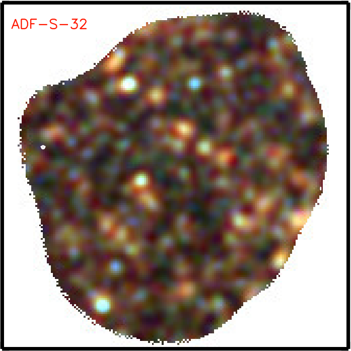
Here we present our LABOCA and Herschel imaging.






Appendix B Photometry and redshift catalogs
Here we present our photometry and photometric redshift catalogs for our sample of ultra-red galaxies and their surrounding DSFGs.
| IAU name | (J2000) | |||||||||||
| mJy | ||||||||||||
| . SGP-28124 . | ||||||||||||
| URG J000124.9354212 | 00:01:24.88 | 35:42:12.2 | 62.2 | 9.1 | 89.8 | 8.8 | 119.9 | 9.3 | 44.3 | 1.4 | 1.04 | 1.00 |
| URG J000145.0353822 | 00:01:44.95 | 35:38:22.1 | 55.9 | 7.9 | 67.4 | 8.6 | 52.4 | 9.4 | 15.9 | 2.6 | 1.15 | 1.00 |
| URG J00014.2354123 | 00:01:04.20 | 35:41:23.0 | 5.9 | 7.5 | 11.7 | 8.8 | 4.7 | 9.7 | 6.4 | 1.5 | 1.35 | 0.97 |
| URG J000122.9354211 | 00:01:22.91 | 35:42:11.2 | 31.9 | 9.0 | 47.9 | 8.7 | 87.8 | 9.4 | 10.2 | 1.4 | 1.11 | 0.92 |
| URG J000138.535442 | 00:01:38.50 | 35:44:02.3 | 4.0 | 9.2 | 9.2 | 9.2 | 3.6 | 10.3 | 4.7 | 1.2 | 1.55 | 0.85 |
| URG J000115.935411 | 00:01:15.90 | 35:41:01.3 | 28.4 | 8.1 | 27.4 | 8.6 | 6.2 | 9.3 | 4.4 | 1.2 | 1.59 | 0.85 |
| URG J000129.4354416 | 00:01:29.39 | 35:44:15.7 | 30.0 | 9.6 | 23.6 | 9.0 | 26.7 | 10.2 | 3.5 | 1.2 | 1.65 | 0.57 |
| . HeLMS-42 . | ||||||||||||
| URG J00034.2024114 | 00:03:04.17 | 02:41:13.7 | 39.8 | 9.2 | 60.3 | 9.9 | 81.0 | 11.3 | 42.6 | 3.6 | 1.89 | 1.00 |
| URG J000319.202371 | 00:03:19.16 | 02:37:00.7 | 1.3 | 8.6 | 3.6 | 8.9 | 1.1 | 11.0 | 24.5 | 6.5 | 5.06 | 0.87 |
| . SGP-93302 . | ||||||||||||
| URG J000624.4323018 | 00:06:24.44 | 32:30:17.7 | 32.1 | 7.1 | 59.6 | 8.3 | 59.6 | 8.9 | 32.0 | 1.3 | 1.03 | 1.00 |
| URG J00067.7322638 | 00:06:07.68 | 32:26:38.0 | 24.0 | 7.7 | 49.7 | 9.3 | 60.9 | 9.1 | 32.4 | 1.9 | 1.03 | 1.00 |
| URG J000621.332328 | 00:06:21.31 | 32:32:07.9 | 15.8 | 7.5 | 27.3 | 7.8 | 22.9 | 8.5 | 13.3 | 1.1 | 1.05 | 1.00 |
| URG J000619.9323126 | 00:06:19.92 | 32:31:26.2 | 23.2 | 7.6 | 21.6 | 8.0 | 21.2 | 8.4 | 5.3 | 1.2 | 1.43 | 0.99 |
| URG J00066.1323016 | 00:06:06.14 | 32:30:16.1 | 40.1 | 7.2 | 23.2 | 8.8 | 13.9 | 8.7 | 7.3 | 1.7 | 1.48 | 0.96 |
| URG J000619.9322847 | 00:06:19.91 | 32:28:46.8 | 23.7 | 7.8 | 23.3 | 8.5 | 18.6 | 8.8 | 4.7 | 1.2 | 1.57 | 0.85 |
| URG J000634.0323138 | 00:06:34.00 | 32:31:38.1 | 11.8 | 7.2 | 10.7 | 7.7 | 10.8 | 8.1 | 4.0 | 1.0 | 1.67 | 0.75 |
| URG J00068.5323338 | 00:06:08.47 | 32:33:38.2 | 6.7 | 7.4 | 6.3 | 8.1 | 5.3 | 8.0 | 5.7 | 1.7 | 1.79 | 0.61 |
| . ELAIS-S1-18 . | ||||||||||||
| URG J002851.3431353 | 00:28:51.31 | 43:13:52.8 | 33.4 | 5.7 | 48.8 | 7.0 | 46.5 | 7.3 | 17.8 | 2.9 | 1.44 | 1.00 |
| URG J00297.7431036 | 00:29:07.74 | 43:10:36.2 | 35.7 | 5.6 | 43.5 | 6.6 | 42.4 | 7.4 | 18.9 | 3.4 | 1.66 | 1.00 |
| URG J002913.443077 | 00:29:13.39 | 43:07:07.0 | 6.7 | 5.1 | 0.2 | 6.2 | 6.5 | 7.1 | 25.1 | 5.9 | 3.20 | 0.99 |
| URG J00294.0430737 | 00:29:03.95 | 43:07:37.2 | 17.7 | 5.8 | 11.1 | 6.6 | 4.2 | 7.2 | 18.0 | 4.6 | 4.60 | 0.87 |
| URG J002919.0430817 | 00:29:19.01 | 43:08:16.8 | 1.6 | 5.3 | 1.8 | 6.2 | 7.7 | 7.5 | 17.5 | 5.9 | 5.29 | 0.69 |
| . ELAIS-S1-26 . | ||||||||||||
| URG J003352.4452015 | 00:33:52.39 | 45:20:14.6 | 24.5 | 6.6 | 37.0 | 8.3 | 43.1 | 9.6 | 12.6 | 2.6 | 1.57 | 1.00 |
| URG J003410.4452230 | 00:34:10.40 | 45:22:29.7 | 45.7 | 9.2 | 37.6 | 9.1 | 18.6 | 10.2 | 14.8 | 3.1 | 1.55 | 1.00 |
| URG J003347.9451441 | 00:33:47.86 | 45:14:40.8 | 11.6 | 6.1 | 20.6 | 6.9 | 13.8 | 7.3 | 15.9 | 4.6 | 3.11 | 0.78 |
| . SGP-208073 . | ||||||||||||
| URG J003533.9280260 | 00:35:33.90 | 28:02:59.5 | 27.7 | 7.7 | 37.4 | 8.8 | 47.6 | 9.7 | 19.2 | 1.8 | 1.16 | 1.00 |
| URG J003540.1280459 | 00:35:40.07 | 28:04:58.7 | 32.3 | 7.6 | 31.2 | 8.5 | 28.1 | 9.8 | 12.4 | 2.0 | 1.22 | 1.00 |
| URG J003536.4280143 | 00:35:36.37 | 28:01:43.3 | 14.7 | 7.9 | 16.8 | 9.0 | 23.4 | 9.7 | 7.1 | 2.0 | 2.23 | 0.72 |
| . ELAIS-S1-29 . | ||||||||||||
| URG J003756.6421519† | 00:37:56.62 | 42:15:19.0 | 24.9 | 6.2 | 35.1 | 7.5 | 43.5 | 8.0 | 7.7 | 2.3 | — | — |
| URG J003831.5421418 | 00:38:31.49 | 42:14:18.4 | 2.3 | 5.7 | 1.8 | 6.6 | 1.4 | 7.3 | 20.0 | 4.8 | 2.02 | 0.95 |
| URG J003744.9421240 | 00:37:44.90 | 42:12:39.6 | 41.7 | 6.7 | 45.8 | 7.7 | 27.8 | 8.3 | 10.3 | 2.7 | 2.59 | 0.90 |
| URG J003811.742198 | 00:38:11.74 | 42:19:08.0 | 0.5 | 5.5 | 0.5 | 6.1 | 0.2 | 7.2 | 16.4 | 4.3 | 2.73 | 0.87 |
| URG J003825.542128 | 00:38:25.48 | 42:12:08.1 | 59.5 | 6.0 | 29.6 | 6.9 | 15.3 | 8.0 | 15.7 | 4.5 | 3.14 | 0.78 |
| URG J00388.4421742 | 00:38:08.44 | 42:17:41.7 | 23.8 | 5.7 | 33.7 | 6.4 | 22.8 | 7.7 | 9.3 | 2.7 | 3.22 | 0.72 |
| . SGP-354388 . | ||||||||||||
| URG J004223.7334325 | 00:42:23.73 | 33:43:25.0 | 15.4 | 8.6 | 47.6 | 8.8 | 59.7 | 9.8 | 34.3 | 1.2 | 1.04 | 1.00 |
| URG J004223.5334350 | 00:42:23.46 | 33:43:49.6 | 23.4 | 8.5 | 35.3 | 8.9 | 33.8 | 9.9 | 17.5 | 1.2 | 1.05 | 1.00 |
| URG J004233.233444 | 00:42:33.16 | 33:44:04.2 | 12.8 | 8.1 | 14.3 | 8.9 | 14.8 | 9.5 | 9.4 | 1.2 | 1.09 | 1.00 |
| URG J004223.2334117 | 00:42:23.25 | 33:41:16.9 | 18.8 | 8.0 | 13.8 | 9.0 | 17.6 | 9.6 | 8.7 | 1.2 | 1.11 | 1.00 |
| URG J004216.1334138 | 00:42:16.11 | 33:41:37.8 | 63.5 | 8.2 | 56.3 | 9.2 | 28.9 | 9.7 | 7.9 | 1.2 | 1.13 | 1.00 |
| URG J004219.8334435 | 00:42:19.79 | 33:44:35.2 | 16.8 | 8.7 | 34.0 | 8.9 | 34.1 | 10.0 | 7.2 | 1.2 | 1.16 | 1.00 |
| URG J004212.9334544 | 00:42:12.86 | 33:45:43.5 | 5.5 | 8.6 | 8.7 | 9.0 | 3.8 | 10.3 | 5.5 | 1.2 | 1.30 | 0.99 |
| URG J004210.1334040 | 00:42:10.09 | 33:40:40.0 | 1.8 | 8.6 | 1.1 | 8.6 | 9.0 | 9.6 | 4.9 | 1.4 | 1.57 | 0.75 |
| URG J004228.5334925 | 00:42:28.53 | 33:49:24.6 | 4.0 | 8.6 | 1.1 | 9.2 | 15.2 | 10.3 | 10.9 | 2.8 | 1.49 | 0.72 |
| . SGP-380990 . | ||||||||||||
| URG J004614.6321828 | 00:46:14.55 | 32:18:28.1 | 20.4 | 8.2 | 43.1 | 8.9 | 46.6 | 9.3 | 10.4 | 1.6 | 1.18 | 1.00 |
| URG J004620.232209 | 00:46:20.19 | 32:20:08.5 | 24.3 | 8.5 | 29.2 | 9.0 | 34.3 | 9.3 | 9.2 | 1.8 | 1.31 | 1.00 |
| URG J00464.4321844 | 00:46:04.41 | 32:18:44.2 | 23.2 | 8.0 | 17.4 | 8.6 | 8.3 | 9.3 | 7.6 | 2.2 | 2.18 | 0.69 |
| . HeLMS-10 . | ||||||||||||
| URG J005258.6061318 | 00:52:58.61 | 06:13:18.2 | 68.9 | 11.5 | 105.4 | 11.2 | 124.3 | 11.7 | 81.7 | 4.7 | 2.19 | 1.00 |
| URG J00532.4061113 | 00:53:02.41 | 06:11:12.9 | 7.3 | 9.8 | 3.7 | 10.7 | 6.7 | 12.3 | 23.8 | 5.8 | 7.62 | 0.98 |
| URG J005310.4061510 | 00:53:10.40 | 06:15:09.5 | 45.3 | 11.4 | 51.6 | 11.8 | 29.5 | 12.5 | 38.3 | 8.4 | 3.59 | 0.98 |
| . SGP-221606 . | ||||||||||||
| URG J011918.9294516 | 01:19:18.93 | 29:45:15.7 | 34.9 | 7.7 | 53.6 | 8.8 | 52.1 | 9.9 | 20.3 | 3.9 | 1.82 | 1.00 |
| URG J011915.9294748 | 01:19:15.86 | 29:47:47.6 | 1.2 | 8.0 | 0.0 | 9.0 | 22.6 | 9.1 | 16.2 | 4.1 | 3.80 | 0.94 |
| URG J01191.8294342 | 01:19:01.83 | 29:43:42.0 | 7.9 | 7.6 | 7.2 | 9.1 | 3.1 | 9.9 | 17.9 | 5.5 | 5.92 | 0.69 |
| URG J01199.6294241 | 01:19:09.59 | 29:42:40.6 | 0.1 | 7.7 | 0.9 | 9.6 | 0.5 | 9.8 | 15.5 | 4.6 | 5.87 | 0.61 |
| . SGP-146631 . | ||||||||||||
| URG J013155.8311147 | 01:31:55.82 | 31:11:47.0 | 26.1 | 7.4 | 32.7 | 7.5 | 39.9 | 8.0 | 15.0 | 3.3 | 1.87 | 0.98 |
| URG J01324.5311239 | 01:32:04.46 | 31:12:38.5 | 47.2 | 7.9 | 78.7 | 7.6 | 67.9 | 8.5 | 11.5 | 3.2 | 3.92 | 0.94 |
| URG J013215.5310837 | 01:32:15.51 | 31:08:36.6 | 5.7 | 8.5 | 8.6 | 8.8 | 6.4 | 9.4 | 14.9 | 4.0 | 3.73 | 0.85 |
| Continued on next page … | ||||||||||||
| IAU name | (J2000) | |||||||||||
| mJy | ||||||||||||
| . SGP-278539 . | ||||||||||||
| URG J01428.2323426† | 01:42:08.20 | 32:34:26.3 | 22.7 | 8.3 | 39.0 | 9.2 | 50.7 | 9.5 | 8.7 | 2.8 | — | — |
| URG J014226.2323324 | 01:42:26.25 | 32:33:23.8 | 7.0 | 8.4 | 2.6 | 8.5 | 8.2 | 9.2 | 17.2 | 3.2 | 1.40 | 1.00 |
| URG J01421.6323624 | 01:42:01.58 | 32:36:23.8 | 6.7 | 8.7 | 7.4 | 9.0 | 9.3 | 9.0 | 14.1 | 2.9 | 1.49 | 0.99 |
| URG J014214.432290 | 01:42:14.41 | 32:29:00.2 | 6.1 | 8.1 | 9.5 | 8.6 | 8.6 | 9.6 | 15.7 | 4.2 | 2.83 | 0.92 |
| URG J014218.232352 | 01:42:18.19 | 32:35:01.5 | 0.1 | 8.3 | 7.2 | 8.7 | 2.8 | 9.2 | 9.6 | 2.8 | 3.26 | 0.65 |
| . SGP-142679 . | ||||||||||||
| URG J014456.9284146 | 01:44:56.88 | 28:41:46.0 | 29.9 | 8.1 | 65.0 | 9.8 | 71.7 | 9.9 | 12.9 | 2.8 | 1.59 | 1.00 |
| URG J014448.8283535 | 01:44:48.78 | 28:35:35.4 | 7.5 | 7.7 | 9.0 | 8.5 | 10.5 | 8.9 | 18.3 | 4.2 | 1.88 | 0.97 |
| URG J01456.7284457 | 01:45:06.66 | 28:44:57.3 | 97.2 | 8.5 | 101.8 | 9.8 | 82.2 | 9.8 | 15.6 | 3.5 | 1.70 | 0.96 |
| . XMM-LSS-15 . | ||||||||||||
| URG J021745.3030912 | 02:17:45.30 | 03:09:12.3 | 12.6 | 6.2 | 22.2 | 7.2 | 24.0 | 7.8 | 17.6 | 3.0 | 1.47 | 1.00 |
| URG J021757.1030753 | 02:17:57.12 | 03:07:53.0 | 56.8 | 6.5 | 34.5 | 7.4 | 14.6 | 7.6 | 11.5 | 2.9 | 2.67 | 0.90 |
| URG J021737.303128 | 02:17:37.29 | 03:12:08.0 | 0.5 | 6.7 | 0.3 | 7.5 | 4.6 | 8.2 | 10.8 | 3.2 | 3.55 | 0.69 |
| . XMM-LSS-30 . | ||||||||||||
| URG J022656.6032711 | 02:26:56.60 | 03:27:11.1 | 25.6 | 6.3 | 44.8 | 7.0 | 61.6 | 7.1 | 23.3 | 2.0 | 1.16 | 1.00 |
| URG J022644.9032510 | 02:26:44.90 | 03:25:10.1 | 44.2 | 6.3 | 65.6 | 6.8 | 63.9 | 7.5 | 18.8 | 2.6 | 1.23 | 1.00 |
| URG J022630.2032530 | 02:26:30.16 | 03:25:30.0 | 20.7 | 5.7 | 24.3 | 7.0 | 18.4 | 7.7 | 29.8 | 6.4 | 2.04 | 0.97 |
| URG J02270.8032541 | 02:27:00.81 | 03:25:41.0 | 10.3 | 6.5 | 10.3 | 7.1 | 13.9 | 7.8 | 7.6 | 2.0 | 3.38 | 0.93 |
| URG J022650.0032542 | 02:26:50.00 | 03:25:41.9 | 28.9 | 6.5 | 28.6 | 6.7 | 18.0 | 7.3 | 7.6 | 2.1 | 3.53 | 0.61 |
| . CDFS-13 . | ||||||||||||
| URG J03370.7292148 | 03:37:00.72 | 29:21:48.0 | 41.1 | 5.9 | 51.0 | 7.1 | 55.4 | 7.2 | 26.2 | 3.5 | 1.45 | 1.00 |
| URG J03370.3291746 | 03:37:00.35 | 29:17:45.8 | 23.3 | 5.8 | 20.6 | 6.8 | 10.5 | 6.8 | 37.6 | 5.9 | 1.45 | 1.00 |
| URG J033655.2292627 | 03:36:55.23 | 29:26:26.9 | 11.6 | 7.3 | 15.7 | 7.3 | 7.6 | 7.0 | 17.8 | 5.0 | 5.46 | 0.75 |
| . ADF-S-27 . | ||||||||||||
| URG J043657.0543813 | 04:36:57.01 | 54:38:13.2 | 16.5 | 6.0 | 24.0 | 7.1 | 28.2 | 7.8 | 25.3 | 1.8 | 1.24 | 1.00 |
| URG J043729.954365 | 04:37:29.90 | 54:36:04.5 | 14.9 | 6.8 | 17.9 | 7.9 | 19.9 | 7.7 | 18.0 | 3.3 | 1.34 | 1.00 |
| URG J04374.7543914 | 04:37:04.65 | 54:39:13.7 | 3.7 | 6.0 | 2.4 | 8.0 | 0.4 | 7.8 | 10.2 | 1.9 | 1.35 | 1.00 |
| URG J043717.454356 | 04:37:17.35 | 54:35:06.2 | 13.5 | 7.1 | 21.7 | 7.9 | 25.5 | 7.6 | 8.8 | 2.4 | 2.35 | 0.98 |
| URG J043717.5543528 | 04:37:17.49 | 54:35:28.3 | 48.7 | 7.1 | 54.5 | 7.8 | 49.0 | 7.6 | 6.2 | 2.3 | 2.59 | 0.93 |
| URG J04377.554341 | 04:37:07.51 | 54:34:00.6 | 34.2 | 6.6 | 27.3 | 7.9 | 13.6 | 7.9 | 8.9 | 2.3 | 2.18 | 0.93 |
| URG J043649.454408 | 04:36:49.44 | 54:40:08.4 | 7.9 | 5.4 | 13.9 | 6.9 | 5.2 | 8.2 | 9.0 | 2.2 | 2.00 | 0.78 |
| . ADF-S-32 . | ||||||||||||
| URG J044410.1534949† | 04:44:10.13 | 53:49:49.1 | 13.1 | 6.0 | 16.6 | 6.8 | 20.8 | 8.0 | 5.5 | 2.8 | — | — |
| URG J04450.453496 | 04:45:00.43 | 53:49:06.2 | 9.3 | 5.6 | 0.9 | 6.8 | 0.6 | 8.0 | 20.0 | 6.0 | 3.81 | 0.78 |
| . G09-83808 . | ||||||||||||
| URG J090045.7004124 | 09:00:45.74 | 00:41:24.1 | 10.9 | 7.5 | 24.1 | 8.3 | 42.4 | 8.7 | 26.3 | 1.3 | 1.06 | 1.00 |
| URG J090032.8004313 | 09:00:32.77 | 00:43:13.0 | 79.5 | 6.6 | 69.2 | 7.7 | 40.9 | 8.1 | 18.5 | 1.4 | 1.06 | 1.00 |
| URG J090019.4004016 | 09:00:19.37 | 00:40:15.7 | 5.6 | 6.4 | 2.3 | 7.4 | 8.1 | 7.3 | 18.3 | 3.3 | 1.18 | 1.00 |
| URG J090057.300415 | 09:00:57.28 | 00:41:04.8 | 30.1 | 7.3 | 32.5 | 8.2 | 28.1 | 9.0 | 5.5 | 1.1 | 1.25 | 1.00 |
| URG J090054.2004343 | 09:00:54.21 | 00:43:43.1 | 19.2 | 7.5 | 18.8 | 8.2 | 19.9 | 8.9 | 3.7 | 1.1 | 1.66 | 0.75 |
| URG J090057.1004039 | 09:00:57.08 | 00:40:39.4 | 26.9 | 7.4 | 33.6 | 8.4 | 32.7 | 9.0 | 3.2 | 1.2 | 1.66 | 0.61 |
| URG J090037.1003624 | 09:00:37.14 | 00:36:24.3 | 72.9 | 6.6 | 65.4 | 7.4 | 43.8 | 8.3 | 8.6 | 2.4 | 1.60 | 0.61 |
| . G15-82684 . | ||||||||||||
| URG J14506.3015038 | 14:50:06.29 | 01:50:38.4 | 31.5 | 7.1 | 37.9 | 7.4 | 45.4 | 8.9 | 17.4 | 1.5 | 1.07 | 1.00 |
| URG J145013.1014810 | 14:50:13.10 | 01:48:09.8 | 17.7 | 7.5 | 36.4 | 8.1 | 39.0 | 9.2 | 17.2 | 1.5 | 1.08 | 1.00 |
| URG J145012.1015158 | 14:50:12.06 | 01:51:57.5 | 30.5 | 7.3 | 34.0 | 7.2 | 34.4 | 8.7 | 11.2 | 1.8 | 1.17 | 1.00 |
| URG J145015.4015237 | 14:50:15.43 | 01:52:37.1 | 18.5 | 7.3 | 33.9 | 7.6 | 37.9 | 8.5 | 13.2 | 2.3 | 1.21 | 1.00 |
| URG J145025.7015115 | 14:50:25.66 | 01:51:14.8 | 21.9 | 7.8 | 31.7 | 7.7 | 22.8 | 9.1 | 7.1 | 1.9 | 1.68 | 1.00 |
| URG J145023.801514 | 14:50:23.82 | 01:51:04.4 | 13.7 | 7.6 | 9.8 | 7.7 | 23.9 | 8.9 | 5.4 | 1.7 | 1.92 | 0.92 |
| . SGP-433089 . | ||||||||||||
| URG J222737.4333835 | 22:27:37.37 | 33:38:34.7 | 28.3 | 9.2 | 36.8 | 10.0 | 35.1 | 10.8 | 8.1 | 1.1 | 1.12 | 1.00 |
| URG J222725.2333920 | 22:27:25.22 | 33:39:19.5 | 35.3 | 9.4 | 38.8 | 10.4 | 20.2 | 11.3 | 8.1 | 1.4 | 1.16 | 1.00 |
| URG J222747.9333533 | 22:27:47.89 | 33:35:32.7 | 21.7 | 9.4 | 32.0 | 9.8 | 25.1 | 10.9 | 7.5 | 1.3 | 1.17 | 1.00 |
| URG J222731.133404 | 22:27:31.09 | 33:40:03.7 | 5.0 | 9.1 | 8.0 | 10.4 | 1.1 | 11.1 | 6.3 | 1.2 | 1.21 | 1.00 |
| URG J222733.7333440 | 22:27:33.67 | 33:34:40.2 | 40.2 | 9.7 | 43.8 | 10.0 | 28.8 | 10.7 | 6.4 | 1.3 | 1.24 | 1.00 |
| URG J222737.7333727 | 22:27:37.70 | 33:37:26.8 | 49.7 | 9.5 | 47.2 | 9.9 | 23.2 | 10.5 | 5.1 | 1.1 | 1.31 | 0.99 |
| URG J222730.4333534 | 22:27:30.44 | 33:35:33.6 | 18.5 | 9.5 | 18.8 | 9.9 | 18.2 | 11.0 | 5.5 | 1.3 | 1.35 | 0.96 |
| URG J222750.1334153 | 22:27:50.14 | 33:41:53.2 | 10.3 | 9.9 | 11.5 | 10.3 | 19.9 | 10.8 | 7.0 | 1.8 | 1.50 | 0.93 |
| URG J222753.8333529 | 22:27:53.81 | 33:35:28.5 | 4.3 | 9.7 | 38.1 | 10.2 | 16.2 | 10.9 | 6.4 | 1.7 | 1.55 | 0.90 |
| URG J222727.8334056 | 22:27:27.79 | 33:40:56.3 | 17.5 | 9.6 | 27.9 | 10.5 | 25.9 | 11.1 | 5.2 | 1.3 | 1.44 | 0.85 |
| URG J222744.7333741 | 22:27:44.74 | 33:37:40.8 | 5.5 | 9.4 | 37.0 | 9.9 | 27.6 | 10.8 | 4.5 | 1.1 | 1.46 | 0.75 |
‡ SPIRE flux densities have been boosted to reflect the radial offset of a LABOCA source. Additionally, flux densities have been deboosted.
† Signpost ultra-red galaxies that are undetected. We report the peak flux density and r.m.s. values for these sources within a aperture centered on the telescope pointing position. We do not provide flux boosting () or fidelity () values.
Note. Targets are listed in order of increasing right ascension and are highlighted in bold. Each source detected in a given field is subsequently listed in increasing order of detected .
| ID | ID | ||||||
| [] | [] | ||||||
| . SGP-28124 . | |||||||
| URG J000124.9354212 | URG J000145.0353822 | 0.19 | |||||
| URG J00014.2354123 | 0.36 | URG J000122.9354211 | 32.37 | ||||
| URG J000138.535442 | 1.02 | URG J000115.935411 | 0.69 | ||||
| URG J000129.4354416 | 2.20 | ||||||
| . HeLMS-42 . | |||||||
| URG J00034.2024114 | URG J000319.202371‡ | — | — | — | |||
| . SGP-93302 . | |||||||
| URG J000624.4323018 | URG J00067.7322638 | 0.02 | |||||
| URG J000621.332328 | 0.26 | URG J000619.9323126 | 0.64 | ||||
| URG J00066.1323016 | 1.05 | URG J000619.9322847 | 0.42 | ||||
| URG J000634.0323138 | 0.13 | URG J00068.5323338‡ | — | — | — | ||
| . ELAISS1-18 . | |||||||
| URG J002851.3431353 | URG J00297.7431036 | 0.81 | |||||
| URG J002913.443077 | 1.38 | URG J00294.0430737 | 0.37 | ||||
| URG J002919.0430817 | 0.75 | ||||||
| . ELAISS1-26 . | |||||||
| URG J003352.4452015 | URG J003410.4452230 | 1.44 | |||||
| URG J003347.9451441 | 0.16 | ||||||
| . SGP-208073 . | |||||||
| URG J003533.9280260 | URG J003540.1280459 | 0.64 | |||||
| URG J003536.4280143 | 1.25 | ||||||
| . ELAISS1-29 . | |||||||
| URG J003756.6421519 | URG J003831.5421418‡ | — | — | — | |||
| URG J003744.9421240 | 1.15 | URG J003811.742198‡ | — | — | — | ||
| URG J003825.542128 | 0.34 | URG J00388.4421742 | 1.66 | ||||
| . SGP-354388 . | |||||||
| URG J004223.7334325 | URG J004223.5334350 | 0.18 | |||||
| URG J004233.233444 | 0.36 | URG J004223.2334117 | 1.09 | ||||
| URG J004216.1334138 | 0.06 | URG J004219.8334435 | 2.39 | ||||
| URG J004212.9334544‡ | — | — | — | URG J004210.1334040‡ | — | — | — |
| URG J004228.5334925‡ | — | — | — | ||||
| . SGP-380990 . | |||||||
| URG J004614.6321828 | URG J004620.232209 | 1.34 | |||||
| URG J00464.4321844 | 0.23 | ||||||
| . HeLMS-10 . | |||||||
| URG J005258.6061318 | URG J00532.4061113‡ | — | — | — | |||
| URG J005310.4061510 | 0.12 | ||||||
| . SGP-221606 . | |||||||
| URG J011918.9294516 | URG J011915.9294748 | 2.72 | |||||
| URG J01191.8294342 | 0.56 | URG J01199.6294241‡ | — | — | — | ||
| . SGP-146631 . | |||||||
| URG J013155.8311147 | 2.26 | URG J01324.5311239 | |||||
| URG J013215.5310837‡ | — | — | — | ||||
| . SGP-278539 . | |||||||
| URG J01428.2323426 | URG J014226.2323324‡ | — | — | — | |||
| URG J01421.6323624 | 0.23 | URG J014214.432290 | 0.06 | ||||
| URG J014218.232352‡ | — | — | — | ||||
| . SGP-142679 . | |||||||
| URG J014456.9284146 | URG J014448.8283535 | 2.69 | |||||
| URG J01456.7284457 | 8.07 | ||||||
| . XMM-15 . | |||||||
| URG J021745.3030912 | URG J021757.1030753 | 0.09 | |||||
| URG J021737.303128‡ | — | — | — | ||||
| . XMM-30 . | |||||||
| URG J022656.6032711 | URG J022644.9032510 | 3.05 | |||||
| URG J022630.2032530 | 1.45 | URG J02270.8032541 | 0.53 | ||||
| URG J022650.0032542 | 0.70 | ||||||
| . CDFS-13 . | |||||||
| URG J03370.7292148 | URG J03370.3291746 | 13.23 | |||||
| URG J033655.2292627 | 0.15 | ||||||
| . ADFS-27 . | |||||||
| URG J043657.0543813 | URG J043729.954365 | 0.80 | |||||
| URG J04374.7543914‡ | — | — | — | URG J043717.454356 | 1.90 | ||
| URG J043717.5543528 | 11.45 | URG J04377.554341 | 0.05 | ||||
| Continued on next page | |||||||
| ID | ID | ||||||
|---|---|---|---|---|---|---|---|
| [] | [] | ||||||
| URG J043649.454408 | 0.54 | ||||||
| . ADFS-32 . | |||||||
| URG J044410.1534949 | URG J04450.453496‡ | — | — | — | |||
| . G09-83808 . | |||||||
| URG J090045.7004124 | URG J090032.8004313 | 6.55 | |||||
| URG J090019.4004016‡ | — | — | — | URG J090057.300415 | 1.20 | ||
| URG J090054.2004343 | 1.16 | URG J090057.1004039 | 6.49 | ||||
| URG J090037.1003624 | 2.45 | ||||||
| . G15-82684 . | |||||||
| URG J14506.3015038 | 1.24 | URG J145013.1014810 | |||||
| URG J145012.1015158 | 0.58 | URG J145015.4015237 | 0.83 | ||||
| URG J145025.7015115 | 0.83 | URG J145023.801514 | 2.67 | ||||
| . SGP-433089 . | |||||||
| URG J222737.4333835 | URG J222725.2333920 | 0.14 | |||||
| URG J222747.9333533 | 0.21 | URG J222731.133404‡ | — | — | — | ||
| URG J222733.7333440 | 0.66 | URG J222737.7333727 | 0.81 | ||||
| URG J222730.4333534 | 0.16 | URG J222750.1334153 | 0.51 | ||||
| URG J222753.8333529 | 4.51 | URG J222727.8334056 | 1.43 | ||||
| URG J222744.7333741 | 6.69 | ||||||
† We quote errors based on the values, without the adding the intrinsic template scatter in quadrature.
‡ SPIRE non-detections, for which we do not provide any photometric redshifts; we do not include these in our analysis.