跳到论文正文
W Papers独立论文阅读器 arXiv:1711.08736 论文正文 计算阅读时间 · 0%
引用这篇论文根据当前论文元数据生成,正式投稿前建议核对。


License: arXiv.org perpetual non-exclusive license
arXiv:1711.08736v2 [math.ST] 22 Sep 2018

Change-point inference on volatility in noisy Itô semimartingales

Markus Bibinger Address: Faculty of Mathematics and Computer Science, Philipps-Universität Marburg    Mehmet Madensoy Note: Madensoy acknowledges financial support from the Deutsche Forschungsgemeinschaft via RTG 1953. Address: School of Business Informatics and Mathematics, Mannheim University
This version: 06.09.2017
Abstract

This work is concerned with tests on structural breaks in the spot volatility process of a general Itô semimartingale based on discrete observations contaminated with i.i.d. microstructure noise. We construct a consistent test building up on infill asymptotic results for certain functionals of spectral spot volatility estimates. A weak limit theorem is established under the null hypothesis relying on extreme value theory. We prove consistency of the test and of an associated estimator for the change point. A simulation study illustrates the finite-sample performance of the method and efficiency gains compared to a skip-sampling approach.

Keywords:
Change-point analysis, high-frequency data , market microstructure , volatility estimation , volatility jump
2010 MSC
62M10 , 62G10

1 Introduction

Inference on structural breaks for discrete-time stochastic processes, particularly in time series analysis, is a very active research field within mathematical statistics. Whereas the latter is usually concerned with i.i.d. data, important contributions beyond that case are presented in Wu and Zhao (2007), proving limit theorems for nonparametric change-point analysis under weak dependence. These results serve as an important ingredient for the present work. So far inference on structural breaks for continuous-time stochastic processes has attracted less attention. Let us mention the very recent work by Bücher et al. (2017), which also deals with questions of detecting structural breaks of certain continuous-time stochastic processes. Our target of inference is the volatility process. Understanding the structure and dynamics of stochastic volatility processes is a highly important issue in finance and econometrics. Due to the outstanding role of volatility for quantifying financial risk, there is a vast literature on these topics.
Motivated by fundamental results in financial mathematics, the process modeling the logarithmic price of an asset belongs to the class of semimartingales. Whereas statistics for general semimartingales is less developed, a lot of work has been done if (Xt)t∈[0,1]\left(X_{t}\right)_{t\in\left[0,1\right]} is an Itô semimartingale, that is, a semimartingale with a characteristic triple being absolutely continuous with respect to the Lebesgue measure. An overview on existing theory is available by Jacod and Protter (2012). More precisely, our continuous-time model is

Xt=Ct+Jt,\displaystyle X_{t}=C_{t}+J_{t}\,, (1)

with (Ct)t∈[0,1]\left(C_{t}\right)_{t\in\left[0,1\right]} the continuous part,

Ct=X0+∫0tσs​d​Ws+∫0tas​𝑑s,\displaystyle C_{t}=X_{0}+\int_{0}^{t}\sigma_{s}\,dW_{s}+\int_{0}^{t}a_{s}\,ds\,, (2)

with a standard Brownian motion (Wt)t∈[0,1]\left(W_{t}\right)_{t\in\left[0,1\right]}, the volatility process (σt)t∈[0,1]\left(\sigma_{t}\right)_{t\in\left[0,1\right]} and the drift process (at)t∈[0,1]\left(a_{t}\right)_{t\in\left[0,1\right]}. We define the pure-jump process (Jt)t∈[0,1]\left(J_{t}\right)_{t\in\left[0,1\right]} through the Grigelionis representation

Jt=∫0t∫ℝδ(s,z)𝟙{|δ(s,z)|≤1}(μ−ν)(ds,dz)+∫0t∫ℝδ(s,z)𝟙{|δ(s,z)|>1}μ(ds,dz)\displaystyle J_{t}=\int_{0}^{t}\int_{\mathbb{R}}\delta(s,z)\mathbbm{1}_{\{|\delta(s,z)|\leq 1\}}(\mu-\nu)(ds,dz)+\int_{0}^{t}\int_{\mathbb{R}}\delta(s,z)\mathbbm{1}_{\{|\delta(s,z)|>1\}}\mu(ds,dz) (3)

with a Poisson random measure μ\mu having a compensator of the form ν⁡(d​s,d​z)=λ⁡(d​z)⊗d​s\nu(ds,dz)=\lambda(dz)\otimes ds with a σ\sigma-finite measure λ\lambda.

In this paper we are going to work with discrete observations and within the framework of infill asymptotics. That is, our data is generated by discretizing a path of the continuous-time stochastic process (Xt)t∈[0,1]\left(X_{t}\right)_{t\in\left[0,1\right]} on a regular, equidistant grid. Though the model (1) is quite flexible, empirical evidence suggests that the recorded financial high-frequency data in applications does not follow a ‘true’ semimartingale. Therefore, an extension of model (1) incorporating microstructure noise is necessary. Market microstructure noise is caused by various trading mechanisms as discreteness of prices and bid-ask spread bounce effects. The observed data is modeled through

Yi​Δn,i=0,…,Δn−1=n∈ℕ,\displaystyle Y_{i\Delta_{n}},\quad i=0,\ldots,\Delta^{-1}_{n}=n\in\mathbb{N}\,, (4)

as a discretization of a continuous-time stochastic process (Yt)t∈[0,1]\left(Y_{t}\right)_{t\in\left[0,1\right]}, given by a superposition

Yt=Xt+εt,\displaystyle Y_{t}=X_{t}+\varepsilon_{t}\,, (5)

with (εt)t∈[0,1]\left(\varepsilon_{t}\right)_{t\in\left[0,1\right]} being a centered white noise process modeling the microstructure noise. This prominent additive noise model has attained considerable attention in the econometrics and statistics literature, let us refer to the book by Aït-Sahalia and Jacod (2014) for an overview. Infill asymptotics implies Δn→0\Delta_{n}\rightarrow 0 or, equivalently, n→+∞n\rightarrow+\infty. Whereas the drift process (at)t∈[0,1]\left(a_{t}\right)_{t\in\left[0,1\right]} is not identifiable in a high-frequency framework, also without noise, quantities as the spot volatility process (σt2)t∈[0,1]\left(\sigma^{2}_{t}\right)_{t\in\left[0,1\right]} and the integrated volatility process ∫0.σ2sds\int_{0}^{.}\sigma^{2}_{s}\,ds, respectively, are identifiable. Since they constitute key quantities for an econometric risk analysis, there exists a rich literature on estimation theory. We refer to Jacod and Protter (2012) for a comprehensive presentation of these topics. This work is aimed to increase the understanding of the structure of the spot volatility process and to complement existing literature. The recent work by Bibinger et al. (2017) presents results on change-point detection for the model (1) without noise. We focus on a test that distinguishes continuous volatility paths from paths with volatility jumps. Inference on volatility jumps is currently of great interest in the literature, see, for instance, Jacod and Todorov (2010) and Tauchen and Todorov (2011). Moreover, it provides a necessary ingredient to analyze possible discontinuous leverage effects, see Aït-Sahalia et al. (2017) for a recent approach to this question. Inference on the volatility poses a challenging statistical problem, the volatility being latent and not directly observable. In the model (5) with microstructure noise, this becomes even more involved. The only work we are aware of addressing inference on volatility jumps in this model is by Bibinger and Winkelmann (2018) who extend the test for contemporaneous price and volatility jumps by Jacod and Todorov (2010) to noisy observations. Restricting to finitely many price-jump times, their results do not render general inference on volatility jumps. In this work we will extend the methods and results presented in Bibinger et al. (2017) in order to construct a general test for volatility jumps based on the model (5). Our statistics are functionals of spectral spot volatility estimates building up on the local Fourier method of moments in Altmeyer and Bibinger (2015) extending the volatility estimation approach introduced by Reiß (2011). While several linear estimators for functionals of the volatility have by now been generalized to noise-robust approaches, the considered change-point test is based on maximum statistics and its extension to an efficient method under noise requires new techniques.

The key theorem for the test is a limit theorem under the null hypothesis with an extreme value limit distribution of Gumbel-type. In particular, a clever rescaling of differences of local spot volatility estimates, quite different from the statistics considered in Bibinger et al. (2017), yields an asymptotic distribution-free test. In a certain sense, our test for volatility jumps complements the prominent Gumbel-test for price jumps proposed by Lee and Mykland (2008) and further studied by Palmes and Woerner (2016a) and Palmes and Woerner (2016b). An extension of the Gumbel-test for price jumps to noisy observations is given in Lee and Mykland (2012). We prove that our Gumbel-test for volatility jumps is consistent. Similar to the price-jump test, it facilitates also detection of the jump times – the change points. One main difficulty to prove the limit theorem is to uniformly control the spot volatility estimation errors.

The paper is organized as follows. Section 2 introduces the testing problem and the assumptions. Section 3 constructs the test. We begin with the test for a continuous semimartingale (Xt)t∈[0,1](X_{t})_{t\in[0,1]} which is then extended to the general case utilizing truncation techniques. Section 4 establishes the asymptotic theory including the limit theorem under the null hypothesis, consistency of the test and consistent estimation of the change point under the alternative hypothesis. In Section 5 we conduct a Monte Carlo simulation study. The main insight is that the new test considerably increases the power compared to (optimally) skip sampling the noisy data to lower frequencies and applying the not noise robust method by Bibinger et al. (2017) directly. Section 6 gathers the proofs.

2 Testing problem and theoretical setup

We will develop a test for volatility jumps. We aim to test for some càdlàg squared volatility process (σt2)t∈[0,1](\sigma_{t}^{2})_{t\in[0,1]} hypotheses of the form

H0:there is no jump in ​σt2vs.\displaystyle H_{0}:\text{there is no jump in }\sigma^{2}_{t}\quad\text{vs.} (6)
H1:there is at least one ​θ∈(0,1)​ such that ​|σθ2−lims→θ,s<θσs2|>0.\displaystyle H_{1}:\text{there is at least one }\theta\in\left(0,1\right)\text{ such that }\big|\sigma^{2}_{\theta}-\lim_{s\to\theta,s<\theta}\sigma_{s}^{2}\big|>0\,.

It is standard in the theory of statistics of high-frequency data to address such questions path-wise. This means that H0H_{0} and H1H_{1} are formulated for one particular path of the squared volatility (σt2​(ω))t∈[0,1](\sigma_{t}^{2}(\omega))_{t\in[0,1]} and we strive to make a decision based on discrete observations of the given path of (Yt​(ω))t∈[0,1](Y_{t}(\omega))_{t\in[0,1]}. The semimartingale (Xt)t∈[0,1]\left(X_{t}\right)_{t\in\left[0,1\right]} is defined on a filtered probability space (Ω(0),ℱ(0),(ℱ(0))t∈[0,1],ℙ(0))(\Omega^{(0)},\mathcal{F}^{(0)},(\mathcal{F}^{(0)})_{t\in\left[0,1\right]},\mathbb{P}^{(0)}). We need further assumptions on the coefficient processes of (Xt)(X_{t}).

Assumption 2.1.

The processes aa and σ\sigma are locally bounded. σ\sigma is almost surely strictly positive, that is, inft∈[0,1]σt2≥K−>0\inf_{t\in[0,1]}\sigma_{t}^{2}\geq K^{-}>0.

Our notation for jump processes follows Jacod and Protter (2012).

Assumption 2.2.

Suppose supω,x|δ⁡(s,x)|/γ⁡(x)\sup_{\omega,x}|\delta(s,x)|/\gamma(x) is locally bounded for some deterministic non-negative function γ\gamma which satisfies for some r∈[0,2]r\in[0,2]:

∫ℝ(1∧γr​(x))​λ​(𝑑x)<∞.\displaystyle\int_{\mathbb{R}}(1\wedge\gamma^{r}(x))\lambda(dx)<\infty\,. (7)

The smaller rr, the more restrictive Assumption 2.2. The case r=0r=0 is tantamount to jumps of finite activity.
On the null hypothesis, we allow for very general and rough continuous stochastic volatility processes.

Hypothesis (H0H_{0}-𝔞\mathfrak{a}).

Under the null hypothesis, the modulus of continuity

wδ​(σ)t=sups,r≤t{|σs−σr|:|s−r|<δ}w_{\delta}(\sigma)_{t}=\sup_{s,r\leq t}\{|\sigma_{s}-\sigma_{r}|:|s-r|<\delta\}

is locally bounded in the sense that there exists 𝔞>0\mathfrak{a}>0 and a sequence of stopping times Tn→∞T_{n}\to\infty, such that wδ​(σ)(Tn∧1)≤Ln​δ𝔞w_{\delta}(\sigma)_{(T_{n}\wedge 1)}\leq L_{n}\delta^{\mathfrak{a}}, for some 𝔞>0\mathfrak{a}>0 and some (almost surely finite) random variables LnL_{n}.

The regularity exponent 𝔞∈(0,1]\mathfrak{a}\in(0,1] is selected for the testing problem. The test can be repeated for different values also. The regularity exponent coincides with a usual Hölder exponent when LnL_{n} is a fix constant. Integrating a sequence LnL_{n} enables us to include stochastic volatility processes in our theory. Since stochastic processes as Brownian motion are not in some fix Hölder class, it is crucial to work with (slightly) more general smoothness classes determined by the exponent 𝔞>0\mathfrak{a}>0 and by LnL_{n}. Observe that if

𝔼⁡[|σt2−σs2|𝔟]≤C​|t−s|γ+𝔞​𝔟,for some ​𝔟,C>0​ and ​γ>1,\displaystyle\mathbb{E}\left[\left|\sigma^{2}_{t}-\sigma^{2}_{s}\right|^{\mathfrak{b}}\right]\leq C\left|t-s\right|^{\gamma+\mathfrak{a}\mathfrak{b}}\,,\text{for some }\mathfrak{b},\,C>0\text{ and }\gamma>1\,,

then the Kolmogorov Čentsov Theorem implies that

limn→+∞ℙ⁡(sups,t∈[0,1]|t−s|≤δ|σt2−σs2|≤Ln​δ𝔞)=1\displaystyle\lim_{n\to+\infty}\mathbb{P}\Big(\sup_{\begin{subarray}{c}s,t\in\left[0,1\right]\\ \left|t-s\right|\leq\delta\end{subarray}}\left|\sigma^{2}_{t}-\sigma^{2}_{s}\right|\leq L_{n}\delta^{\mathfrak{a}}\Big)=1

if Ln→+∞L_{n}\rightarrow+\infty arbitrarily slowly. In particular, we can impose that Ln=𝒪⁡(log⁡(n))L_{n}=\mathcal{O}(\log(n)) for our derivation of upper bounds in the sections below. The null hypothesis is the same as in Assumption 3.1 of Bibinger et al. (2017). Our test distinguishes the null hypothesis from alternative hypotheses of the following type.

Alternative (H1H_{1}-𝔞\mathfrak{a}).

Under the alternative hypothesis, there exists at least one θ∈(0,1)\theta\in\left(0,1\right), such that

|Δ​σθ2|=|σθ2−lims→θ,s<θσs2|=δ>0.\big|\Delta\sigma_{\theta}^{2}\big|=\big|\sigma_{\theta}^{2}-\lim_{s\to\theta,s<\theta}\sigma_{s}^{2}\big|=\delta>0\,.

We suppose that σt2=σt2,(c)+σt2,(j)\sigma_{t}^{2}=\sigma_{t}^{2,(c)}+\sigma_{t}^{2,(j)}, where (σt2,(c))t∈[0,1](\sigma_{t}^{2,(c)})_{t\in[0,1]} satisfies ( H 0 - a ). The jump component (σt2,(j))t∈[0,1](\sigma_{t}^{2,(j)})_{t\in[0,1]} is a pure-jump semimartingale which satisfies Assumption 2.2 with r≤2r\leq 2.

In particular, the alternative hypothesis does not restrict to only one jump. We establish a consistent test when at least one non-negligible jump is present. Multiple jumps and quite general jump components are possible. Consistency of our test only requires that in a small vicinity of θ\theta, (σt2,(c))(\sigma_{t}^{2,(c)}) and (σt2,(j)−Δ​σθ2​𝟙[θ,1]​(t))(\sigma_{t}^{2,(j)}-\Delta\sigma_{\theta}^{2}\mathbbm{1}_{[\theta,1]}(t)) are sufficiently regular such that the jump Δ​σθ2\Delta\sigma_{\theta}^{2} is detected. Bibinger et al. (2017) impose in their Theorem 4.3 the condition that all volatility jumps are positive. This condition is replaced here by the semimartingale assumption on (σt2,(j))t∈[0,1](\sigma_{t}^{2,(j)})_{t\in[0,1]}. Both ensure that Δ​σθ2\Delta\sigma_{\theta}^{2} can not be compensated by opposite jumps in an asymptotically small vicinity. In order to incorporate microstructure noise, we have to extend the original probability space. We set 𝒢t=ℱt(0)⊗σ(εs:s≤t)\mathcal{G}_{t}=\mathcal{F}^{(0)}_{t}\otimes\sigma\left(\varepsilon_{s}:\,s\leq t\right). The data generating process (Yt)t∈[0,1]\left(Y_{t}\right)_{t\in\left[0,1\right]} is defined on the filtered probability space (Ω,𝒢,(𝒢t)t∈[0,1],ℙ)\left(\Omega,\mathcal{G},(\mathcal{G}_{t})_{t\in\left[0,1\right]},\mathbb{P}\right). The construction can be pursued such that the process (Xt)t∈[0,1](X_{t})_{t\in[0,1]} remains a semimartingale on the extension with the same characteristic triplet and the same Grigelionis representation. For the details of the construction we refer to Chapter 16 in Jacod and Protter (2012). For the noise process, we impose further assumptions.

Assumption 2.3.

The stochastic process (εt)t∈[0,1]\left(\varepsilon_{t}\right)_{t\in\left[0,1\right]} is defined on (Ω,𝒢,(𝒢t)t∈[0,1],ℙ)\left(\Omega,\mathcal{G},(\mathcal{G}_{t})_{t\in\left[0,1\right]},\mathbb{P}\right) and fulfills the following conditions.

  1. (1)

    (εt)t∈[0,1]\left(\varepsilon_{t}\right)_{t\in\left[0,1\right]} is a centered white noise process, 𝔼⁡[εt]≡0\mathbb{E}[\varepsilon_{t}]\equiv 0, and with

    𝔼⁡[εt2]=η2.\displaystyle\mathbb{E}\left[\varepsilon^{2}_{t}\right]=\eta^{2}\,.
  2. (2)

    The following moment condition holds.

    𝔼⁡[|εt|m]<∞, for all ​m∈ℕ.\displaystyle\mathbb{E}\left[\left|\varepsilon_{t}\right|^{m}\right]<\infty,\text{ for all }m\in\mathbb{N}. (8)

It is well-known that η2\eta^{2} can be estimated in this model with n\sqrt{n}-rate by either a rescaled realized volatility or from the negative first-lag autocovariances of the noisy increments. Under Assumption 2.3, Zhang et al. (2005) provide a rate-optimal consistent estimator for η2\eta^{2}:

η^2=12​n∑i=1n(Yi​Δn−Y(i−1)​Δn)2=η2+𝒪ℙ(n−1/2).\displaystyle\hat{\eta}^{2}=\frac{1}{2n}\sum_{i=1}^{n}(Y_{i\Delta_{n}}-Y_{(i-1)\Delta_{n}})^{2}=\eta^{2}+\mathcal{O}_{\mathbb{P}}\big(n^{-1/2}\big)\,. (9)
Remark 2.4.

The moment condition (8) is standard in related literature, see, for instance, Assumption (WN) of (Aït-Sahalia and Jacod, 2014, page 221) or Assumption 16.1.1 of Jacod and Protter (2012), but in a certain sense purely technical. Let us stress that in our setting, we do impose as less assumptions as possible on the volatility process (σt)t∈[0,1]\left(\sigma_{t}\right)_{t\in\left[0,1\right]}. More precisely, the regularity under ( H 0 - a ), for arbitrarily small 𝔞∈(0,1]\mathfrak{a}\in\left(0,1\right], requires the existence of all moments in (8). More precisely, the smaller 𝔞\mathfrak{a}, the larger mm has to be chosen. Nevertheless, we point out that the moment condition is not that restrictive for standard models of volatility. In the usual case, for instance, where (σt)t∈[0,1]\left(\sigma_{t}\right)_{t\in\left[0,1\right]} itself is assumed to be an Itô semimartingale, when 𝔞≈1/2\mathfrak{a}\approx 1/2, only the existence of moments up to order m=8m=8 has to be imposed.

Remark 2.5.

While Assumption 2.3 is in line with standard conditions on the additive noise component in the literature, possible generalizations with respect to the structure of the noise process (εt)t∈[0,1](\varepsilon_{t})_{t\in\left[0,1\right]} in three directions are of interest: serial dependence, heterogeneity and endogeneity. Such generalizations are also motivated by stylized facts in econometrics, see Hansen and Lunde (2006) for a detailed discussion. For instance, Chapter 16 in Jacod and Protter (2012) includes conditional i.i.d. noise, endogenous as it may depend (in a certain way) on (Xt)(X_{t}), in the theory of pre-average estimators. This allows to model phenomena as noise by price discreteness (rounding). Bibinger and Winkelmann (2018) provide some first extensions of spectral spot volatility estimation to serially correlated and heterogeneous noise. Though the possible extensions appear to be relevant for applications, we work in the framework formulated in Assumption 2.3, mainly due to the lack of groundwork sufficient for the present work. Since we exploit some ingredients from previous works on spectral volatility estimation, particularly the form of the efficient asymptotic variance based on Altmeyer and Bibinger (2015), a generalization of our results requires non-trivial generalizations of these ingredients first. Furthermore, more general noise processes ask for extensive work on the estimation of the local long-run variance replacing (9). This topic, however, is beyond the scope of this work. Let us remark that it is as well not obvious how to apply strong embedding principles in these cases to generalize our proofs. Since Wu and Zhao (2007) provide strong approximation results for weakly dependent time series, we nevertheless conjecture that certain generalizations in the three directions are possible.

3 The statistical methods

3.1 The continuous case

In this paragraph, we construct the test first for the model (Xt)t∈[0,1]\left(X_{t}\right)_{t\in\left[0,1\right]} without jumps, that is, we assume that

Jt≡0.\displaystyle J_{t}\equiv 0.

The construction of the test is based on a combination of the techniques by Altmeyer and Bibinger (2015) and Bibinger et al. (2017). In order to do so, we pick a sequence hnh_{n} with

hn∝n−1/2log(n)\displaystyle h_{n}\varpropto n^{-1/2}\log\left(n\right) (10)

and hn−1∈ℕh_{n}^{-1}\in\mathbb{N}.
The observation interval [0,1]\left[0,1\right] is split into hn−1h_{n}^{-1} bins of length hnh_{n}, such that each bin is given by

[(k−1)​hn,k​hn],k=1,…,hn−1.\displaystyle\left[\left(k-1\right)h_{n},kh_{n}\right],\quad k=1,\ldots,h_{n}^{-1}.

Furthermore, we consider the L2​([0,1])L^{2}\left(\left[0,1\right]\right) orthonormal systems, given by

Φj​k​(t)\displaystyle\Phi_{jk}\left(t\right) =Φj​(t−(k−1)​hn)\displaystyle=\Phi_{j}\left(t-\left(k-1\right)h_{n}\right)
φj​k​(t)\displaystyle\varphi_{jk}\left(t\right) =φj​(t−(k−1)​hn)\displaystyle=\varphi_{j}\left(t-\left(k-1\right)h_{n}\right)

with

Φj​(t)\displaystyle\Phi_{j}\left(t\right) =2hn​sin⁡(j​π​hn−1​t)​𝟙[0,hn]​(t),j≥0,0≤t≤1,\displaystyle=\sqrt{\frac{2}{h_{n}}}\sin\left(j\pi h_{n}^{-1}t\right)\mathbbm{1}_{\left[0,h_{n}\right]}\left(t\right),\quad j\geq 0,0\leq t\leq 1\,,
φj​(t)\displaystyle\varphi_{j}\left(t\right) =2​n​2hn​sin⁡(j​π2​n​hn)​cos⁡(j​π​hn−1​t)​𝟙[0,hn]​(t).\displaystyle=2n\sqrt{\frac{2}{h_{n}}}\sin\left(\frac{j\pi}{2nh_{n}}\right)\cos\left(j\pi h_{n}^{-1}t\right)\mathbbm{1}_{\left[0,h_{n}\right]}\left(t\right).

We define, for any stochastic process (Lt)t∈[0,1]\left(L_{t}\right)_{t\in\left[0,1\right]}, the increments Δin​L\Delta_{i}^{n}L by

ΔinL=Lin−Li−1n,i=1,…,n,\displaystyle\Delta_{i}^{n}L=L_{\frac{i}{n}}-L_{\frac{i-1}{n}}\,,i=1,\ldots,n,

and the spectral statistics

Sj​k​(L):=∑i=1nΔin​L​Φj​k​(in).\displaystyle S_{jk}\left(L\right):=\sum_{i=1}^{n}\Delta_{i}^{n}L\,\Phi_{jk}\left(\frac{i}{n}\right).

The squared volatility σ(k−1)​hn2\sigma^{2}_{\left(k-1\right)h_{n}} can be estimated locally by a parametric estimator through oracle versions of bias corrected linear combinations of the squared spectral statistics,

σ^(k−1)​hn2=∑j=1⌊n​hn⌋−1wj​k​(Sj​k2​(Y)−[φj​k,φj​k]n​η2n),\displaystyle\hat{\sigma}^{2}_{\left(k-1\right)h_{n}}=\sum_{j=1}^{{\lfloor nh_{n}\rfloor}-1}w_{jk}\left(S^{2}_{jk}\left(Y\right)-\left[\varphi_{jk},\varphi_{jk}\right]_{n}\frac{\eta^{2}}{n}\right)\,, (11)

with variance minimizing oracle weights wj​kw_{jk}, given by

wj​k=(σ(k−1)​hn2+η2n​[φj​k,φj​k]n)−2∑m=1⌊n​hn⌋−1(σ(k−1)​hn2+η2n​[φm​k,φm​k]n)−2.\displaystyle w_{jk}=\frac{\left(\sigma^{2}_{\left(k-1\right)h_{n}}+\frac{\eta^{2}}{n}\left[\varphi_{jk},\varphi_{jk}\right]_{n}\right)^{-2}}{\sum_{m=1}^{{\lfloor nh_{n}\rfloor}-1}\left(\sigma^{2}_{\left(k-1\right)h_{n}}+\frac{\eta^{2}}{n}\left[\varphi_{mk},\varphi_{mk}\right]_{n}\right)^{-2}}\,. (12)

The empirical scalar products [f,g]n\left[f,g\right]_{n}, for any functions ff and gg, are given by

[f,g]n=1n​∑i=1nf⁡(i−12n)​g​(i−12n).\displaystyle\left[f,g\right]_{n}=\frac{1}{n}\sum_{i=1}^{n}f\left(\frac{i-\frac{1}{2}}{n}\right)g\left(\frac{i-\frac{1}{2}}{n}\right).

The order in (10) ensures that the error by discretization of the signal part and the error due to noise are balanced.
In a second step we split the observation interval [0,1]\left[0,1\right] by some “big blocks” with length αn​hn\alpha_{n}h_{n}:

[i​αn​hn,(i+1)​αn​hn],i=0,…,⌊(αn​hn)−1⌋−1,\displaystyle\left[i\alpha_{n}h_{n},\left(i+1\right)\alpha_{n}h_{n}\right],\quad i=0,\ldots,{\lfloor\left(\alpha_{n}h_{n}\right)^{-1}\rfloor}-1,

where (αn)n∈ℕ\left(\alpha_{n}\right)_{n\in\mathbb{N}} is some ℕ\mathbb{N}-valued sequence fulfilling as n→+∞n\rightarrow+\infty:

αn​(αn​hn)𝔞​log⁡(n)⟶0​ and ​hn−ϖ/αn⟶0\displaystyle\sqrt{\alpha_{n}}\left(\alpha_{n}h_{n}\right)^{\mathfrak{a}}\sqrt{\log\left(n\right)}\longrightarrow 0\text{ and }h_{n}^{-\varpi}/\alpha_{n}\longrightarrow 0 (13)

for some ϖ>0\varpi>0 and the regularity exponent 𝔞∈(0,1]\mathfrak{a}\in\left(0,1\right] under the null hypothesis ( H 0 - a ). Using spectral estimators and averaging within each big block [i​αn​hn,(i+1)​αn​hn]\left[i\alpha_{n}h_{n},\left(i+1\right)\alpha_{n}h_{n}\right] provides a consistent estimator for σi​αn​hn2\sigma^{2}_{i\alpha_{n}h_{n}}:

R​V¯n,i=1αn∑ℓ=1αnσ^hn​(i​αn+(ℓ−1))2,i=0,…,⌊(αnhn)−1⌋−1.\displaystyle\overline{RV}_{n,i}=\frac{1}{\alpha_{n}}\sum_{\ell=1}^{\alpha_{n}}\hat{\sigma}^{2}_{h_{n}(i\alpha_{n}+\left(\ell-1\right))},\quad i=0,\ldots,{\lfloor\left(\alpha_{n}h_{n}\right)^{-1}\rfloor}-1\,. (14)

A feasible adaptive estimation is obtained by a two-stage method where η^2\hat{\eta}^{2} from (9) and

1αn​∑l=k−αn∨0(k−1)∨(αn−1)∑j=1J1J​(Sj​l2​(Y)−[φj​l,φj​l]n​η^2n)=σ(k−1)​hn2+𝒪ℙ​(1)\displaystyle\frac{1}{\alpha_{n}}\sum_{l=k-\alpha_{n}\vee 0}^{(k-1)\vee(\alpha_{n}-1)}\,\sum_{j=1}^{J}\frac{1}{J}\left(S^{2}_{jl}\left(Y\right)-\left[\varphi_{jl},\varphi_{jl}\right]_{n}\frac{\hat{\eta}^{2}}{n}\right)=\sigma^{2}_{(k-1)h_{n}}+{\scriptstyle{\mathcal{O}}}_{\mathbb{P}}(1) (15)

are inserted in the oracle weights to derive feasible estimated weights w^j​k\hat{w}_{jk}. The result (15) has been established and used in previous works on spectral volatility estimation, see Bibinger and Winkelmann (2018). The pilot volatility estimator (15) is an average of squared bias corrected spectral statistics over JJ Fourier frequencies and αn\alpha_{n} bins. For some fix J∈ℕJ\in\mathbb{N} and an optimal choice of αn∝n𝔞/(2​𝔞+1)/log⁡(n)\alpha_{n}\propto n^{\mathfrak{a}/(2\mathfrak{a}+1)}/\log(n), it renders a rate-optimal estimator for which the 𝒪ℙ​(1){\scriptstyle{\mathcal{O}}}_{\mathbb{P}}(1)-term in (15) is 𝒪ℙ(n−𝔞/(4𝔞+2))\mathcal{O}_{\mathbb{P}}(n^{-\mathfrak{a}/(4\mathfrak{a}+2)}). A sub-optimal choice of αn\alpha_{n} will not affect our results, however. Other weights than (12) do not yield an asymptotically efficient estimator with minimal asymptotic variance. With estimated versions of the optimal weights (12), Altmeyer and Bibinger (2015) show that a Riemann sum over the estimates (11) yields a quasi-efficient estimator for the integrated squared volatility. Hence, we use the statistics (11) with exactly these weights and the orthogonal sine basis (Φj​k)(\Phi_{jk}) motivated by the efficiency results of Reiß (2011). Finally, with adaptive versions of the local volatility estimators (14)

R​V¯n,ia​d\displaystyle\overline{RV}_{n,i}^{ad} =1αn∑ℓ=1αnσ^hn​(i​αn+(ℓ−1))2,a​d,i=0,…,⌊(αnhn)−1⌋−1,\displaystyle=\frac{1}{\alpha_{n}}\sum_{\ell=1}^{\alpha_{n}}\hat{\sigma}^{2,ad}_{h_{n}(i\alpha_{n}+\left(\ell-1\right))},\quad i=0,\ldots,{\lfloor\left(\alpha_{n}h_{n}\right)^{-1}\rfloor}-1\,, (16)
σ^(k−1)​hn2,a​d\displaystyle\hat{\sigma}^{2,ad}_{(k-1)h_{n}} =∑j=1⌊n​hn⌋−1w^j​k​(Sj​k2​(Y)−[φj​k,φj​k]n​η^2n),\displaystyle=\sum_{j=1}^{{\lfloor nh_{n}\rfloor}-1}\hat{w}_{jk}\left(S^{2}_{jk}\left(Y\right)-\left[\varphi_{jk},\varphi_{jk}\right]_{n}\frac{\hat{\eta}^{2}}{n}\right)\,,

our test statistic is given by

V¯n=maxi=0,…,⌊(αn​hn)−1⌋−2|R​V¯n,ia​d−R​V¯n,i+1a​d8​η^​|R​V¯n,i+1a​d|3/4|,\displaystyle\overline{V}_{n}=\mathop{\mathrm{max}}\limits_{i=0,\ldots,{\lfloor\left(\alpha_{n}h_{n}\right)^{-1}\rfloor}-2}\left|\frac{\overline{RV}_{n,i}^{ad}-\overline{RV}_{n,i+1}^{ad}}{\sqrt{8\hat{\eta}}\;\big|\overline{RV}^{ad}_{n,i+1}\big|^{3/4}}\right|\,, (17)

where η^=η^2\hat{\eta}=\sqrt{\hat{\eta}^{2}}, with η^2\hat{\eta}^{2} from (9). We write the absolute value in the denominator, since due to the bias correction in (11) the statistics (R​V¯n,i)(\overline{RV}_{n,i}) and (R​V¯n,ia​d),i=0,…,⌊(αn​hn)−1⌋−1(\overline{RV}^{ad}_{n,i}),i=0,\ldots,{\lfloor\left(\alpha_{n}h_{n}\right)^{-1}\rfloor}-1 are not guaranteed to be positive.

Remark 3.1.
  1. 1.

    The construction of the test statistic (17) is based on the idea to compare the values of the spot volatility process (σt2)t∈[0,1]\left(\sigma^{2}_{t}\right)_{t\in\left[0,1\right]} on intervals [i​αn​hn,(i+1)​αn​hn]\left[i\alpha_{n}h_{n},\left(i+1\right)\alpha_{n}h_{n}\right] and [(i+1)​αn​hn,(i+2)​αn​hn]\left[\left(i+1\right)\alpha_{n}h_{n},\left(i+2\right)\alpha_{n}h_{n}\right] and to reject the null hypothesis of no jumps, if the test statistic V¯n\overline{V}_{n} fulfills V¯n≥cn\overline{V}_{n}\geq c_{n} for some accurate sequence cnc_{n}.

  2. 2.

    The statistic (17) significantly differs from the statistic VnV_{n} given in Equation (13) of Bibinger et al. (2017) beyond replacing spot volatility estimates by noise-robust spot volatility estimates. Though both statistics are quotients, the underlying structure of them is different. Whereas in Bibinger et al. (2017) the simple structure of the (asymptotic) variance of spot volatility estimates allows to use statistics based on their quotients, (17) is based on differences rescaled with their estimated variances. The statistics which are used to wipe out the influence of the noise process imply that volatility does not simply “cancel out” in our case as in Proposition A.3 of Bibinger et al. (2017). The construction of (17) is particularly appropriate from an implementation point of view, since it scales to obtain an asymptotic distribution-free test and makes it possible to avoid pre-estimation of higher order moments.∎

In order to increase the performance of the statistic, we also include a statistic V¯no​v\overline{V}^{ov}_{n} based on overlapping big blocks:

V¯no​v=maxi=αn,…,hn−1−αn|R​V¯n,io​v−R​V¯n,i+αno​v8​η^​|R​V¯n,i+αno​v|3/4|.\displaystyle\overline{V}^{ov}_{n}=\mathop{\mathrm{max}}\limits_{i=\alpha_{n},\ldots,h_{n}^{-1}-\alpha_{n}}\left|\frac{\overline{RV}^{ov}_{n,i}-\overline{RV}^{ov}_{n,i+\alpha_{n}}}{\sqrt{8\hat{\eta}}\;\big|\overline{RV}^{ov}_{n,i+\alpha_{n}}\big|^{3/4}}\right|. (18)

with R​V¯n,io​v\overline{RV}^{ov}_{n,i} given by

R​V¯o​vn,i=1αn∑ℓ=i−αn+1iσ^2,a​d(ℓ−1)​hn,i=αn,…,hn−1.\displaystyle\overline{RV}^{ov}_{n,i}=\frac{1}{\alpha_{n}}\sum_{\ell=i-\alpha_{n}+1}^{i}\hat{\sigma}^{2,ad}_{\left(\ell-1\right)h_{n}},\quad i=\alpha_{n},\ldots,h_{n}^{-1}\,.

3.2 The discontinuous case

In this paragraph, we generalize the method to be robust in the presence of jumps in (1). When (σt)t∈[0,1](\sigma_{t})_{t\in[0,1]} is our target of inference, the jumps are a nuisance quantity. In order to eliminate jumps of (Xt)t∈[0,1](X_{t})_{t\in[0,1]} in the approach, we consider truncated spot volatility estimates

R​V¯n,it​r=1αn∑ℓ=i−αn+1iσ^2,a​d(ℓ−1)​hn𝟙{|σ^2,a​d(ℓ−1)​hn|≤hnτ−1},i=αn,…,hn−1,\displaystyle\overline{RV}_{n,i}^{tr}=\frac{1}{\alpha_{n}}\sum_{\ell=i-\alpha_{n}+1}^{i}\hat{\sigma}^{2,ad}_{\left(\ell-1\right)h_{n}}\mathbbm{1}_{\{|\hat{\sigma}^{2,ad}_{\left(\ell-1\right)h_{n}}|\leq h_{n}^{\tau-1}\}},\quad i=\alpha_{n},\ldots,h_{n}^{-1}\,, (19)

with a truncation exponent τ∈(0,1)\tau\in(0,1). Truncated volatility estimators have been introduced first for integrated volatility estimation by Mancini (2009) and Jacod (2008). We define the test statistics with the truncated spot volatility estimates (19)

V¯nτ\displaystyle\overline{V}_{n}^{\tau} =maxi=1,…,⌊(αn​hn)−1⌋−1|R​V¯n,i​αnt​r−R​V¯n,(i+1)​αnt​r8​η^​|R​V¯n,(i+1)​αnt​r|3/4|,\displaystyle=\mathop{\mathrm{max}}\limits_{i=1,\ldots,{\lfloor\left(\alpha_{n}h_{n}\right)^{-1}\rfloor}-1}\left|\frac{\overline{RV}_{n,i\alpha_{n}}^{tr}-\overline{RV}_{n,(i+1)\alpha_{n}}^{tr}}{\sqrt{8\hat{\eta}}\;\big|\overline{RV}^{tr}_{n,(i+1)\alpha_{n}}\big|^{3/4}}\right|\,, (20a)
V¯no​v,τ\displaystyle\overline{V}^{ov,\tau}_{n} =maxi=αn,…,hn−1−αn|R​V¯n,it​r−R​V¯n,i+αnt​r8​η^​|R​V¯n,i+αnt​r|3/4|.\displaystyle=\mathop{\mathrm{max}}\limits_{i=\alpha_{n},\ldots,h_{n}^{-1}-\alpha_{n}}\left|\frac{\overline{RV}_{n,i}^{tr}-\overline{RV}_{n,i+\alpha_{n}}^{tr}}{\sqrt{8\hat{\eta}}\;\big|\overline{RV}^{tr}_{n,i+\alpha_{n}}\big|^{3/4}}\right|\,. (20b)

4 Asymptotic theory

4.1 Limit theorem under the null hypothesis

The hypothesis test formulated in Section 2 is based on asymptotic results for the statistics V¯n\overline{V}_{n} and V¯no​v\overline{V}^{ov}_{n}, constructed in Section 3.

Theorem 4.1.

Set mn=⌊(αn​hn)−1⌋m_{n}=\lfloor\left(\alpha_{n}h_{n}\right)^{-1}\rfloor, γmn=[4​log⁡(mn)−2​log⁡(log⁡(mn))]1/2\gamma_{m_{n}}=[4\log(m_{n})-2\log(\log(m_{n}))]^{1/2} and assume that Jt≡0J_{t}\equiv 0. If Assumptions 2.1 and 2.3 hold and αn\alpha_{n} satisfies condition (13), then we have under ( H 0 - a ) that

log⁡(mn)​(αn​V¯n−γmn)​⟶d​V\displaystyle\sqrt{\log\left(m_{n}\right)}\left(\sqrt{\alpha_{n}}\overline{V}_{n}-\gamma_{m_{n}}\right)\overset{\mathrm{d}}{\longrightarrow}V (21)

where VV follows an extreme value distribution with distribution function

ℙ(V≤x)=exp(−π−1/2exp(−x)).\displaystyle\mathbb{P}(V\leq x)=\exp(-\pi^{-1/2}\exp(-x)).\

Theorem 4.1 is a key tool tackling the testing problem which is based on non-overlapping big blocks. The following result covers the case of overlapping big blocks.

Corollary 4.2.

Given the assumptions of Theorem 4.1, the following weak convergence holds under ( H 0 - a ):

log⁡(mn)​αn​V¯no​v−2​log⁡(mn)−12​log⁡(log⁡(mn))−log⁡(3)​⟶d​V,\displaystyle\sqrt{\log\left(m_{n}\right)}\sqrt{\alpha_{n}}\overline{V}^{ov}_{n}-2\log\left(m_{n}\right)-\frac{1}{2}\log\left(\log\left(m_{n}\right)\right)-\log\left(3\right)\overset{\mathrm{d}}{\longrightarrow}V, (22)

with VV as in Theorem 4.1.

We extend this result to the setup with jumps in (Xt)t∈[0,1](X_{t})_{t\in[0,1]} when using truncated functionals.

Proposition 4.3.

Let mnm_{n} and γmn\gamma_{m_{n}} be the sequences defined in Theorem 4.1. Suppose αn=κ​hn−β\alpha_{n}=\kappa h_{n}^{-\beta} for a constant κ\kappa and with 0<β<10<\beta<1, Assumption 2.1, Assumption 2.3 and Assumption 2.2 with

r<min⁡(2−βτ,2​τ−1​(1−β),τ−1,34​(1+τ−β2)).\displaystyle r<\min{\Big(2-\frac{\beta}{\tau},2\tau^{-1}(1-\beta),\tau^{-1},\frac{3}{4}\big(1+\tau-\frac{\beta}{2}\big)\Big)}\,. (23)

Then we have under ( H 0 - a ) that

log⁡(mn)​(αn​V¯nτ−γmn)​⟶d​V,\displaystyle\sqrt{\log\left(m_{n}\right)}\left(\sqrt{\alpha_{n}}\,\overline{V}^{\tau}_{n}-\gamma_{m_{n}}\right)\overset{\mathrm{d}}{\longrightarrow}V\,, (24a)
log⁡(mn)​αn​V¯no​v,τ−2​log⁡(mn)−12​log⁡(log⁡(mn))−log⁡(3)​⟶d​V,\displaystyle\sqrt{\log\left(m_{n}\right)}\sqrt{\alpha_{n}}\,\overline{V}^{ov,\tau}_{n}-2\log\left(m_{n}\right)-\frac{1}{2}\log\left(\log\left(m_{n}\right)\right)-\log\left(3\right)\overset{\mathrm{d}}{\longrightarrow}V\,, (24b)

with VV as in Theorem 4.1.

It is natural that we derive the same limit results as above, since the truncation aims to eliminate the nuisance jumps. Proposition 4.3 gives rather minimal conditions, in particular (23), under that we can guarantee that the truncation works in this sense.

Remark 4.4.

Condition (23) ensures that different error terms in the proof of Proposition 4.3 are asymptotically negligible. Though we state it in terms of upper bounds on the jump activity rr, it rather puts restrictions on the interplay between rr, τ\tau and β\beta. Given 𝔞\mathfrak{a} from ( H 0 - a ), we choose β\beta close to 2​𝔞/(2​𝔞+1)2\mathfrak{a}/(2\mathfrak{a}+1) to attain the highest possible power of the test. This results in 0<β<2/30<\beta<2/3, where the case β≈1/2\beta\approx 1/2 for 𝔞=1/2\mathfrak{a}=1/2 appears the most relevant one including a test for jumps in a semimartingale volatility process. Rewritten in terms of bounds on τ\tau, (23) gives:

max⁡(β2−r,43​r+β2−1)<τ<min⁡(r−1,2​r−1​(1−β)).\max\Big(\frac{\beta}{2-r},\frac{4}{3}r+\frac{\beta}{2}-1\Big)<\tau<\min\Big(r^{-1},2r^{-1}(1-\beta)\Big)\,.

For finite activity, r=0r=0, we only have mild lower bounds on the choice of τ\tau. Usually, a choice of τ\tau close to 1 is advocated in previous works on truncated volatility estimation. For β≈1/2\beta\approx 1/2, this requires r<1r<1. The different error terms under noise for the maximum obtained here actually suggest that τ=3/4\tau=3/4 is an even better choice when we require only r<4/3r<4/3. Overall, the conditions on the jumps are not much more restrictive than required for central limit theorems of linear volatility estimators, see Chapter 13 of Jacod and Protter (2012). Compared to Proposition 3.5 of Bibinger et al. (2017), we relax the conditions on (Jt)(J_{t}) by a more sophisticated strategy of our proof. In particular, we do not have to restrict to a Lévy-type process with independent increments, since we work with Doob’s submartingale maximal inequality instead of Kolmogorov’s maximal inequality. With this strategy it is also possible to generalize the result in Proposition 3.5 of Bibinger et al. (2017).

4.2 Key ideas of the proof of the limit results

Since the proofs of the results stated in Section 4.1 are quite long, we want to sketch the key ideas of the proof shortly. The details are worked out in Section 6.
Starting with the continuous case, for the results given in Theorem 4.1 and Corollary 4.2, the main ingredients are described as follows. In the first step we carry out the crucial approximation where we show that the error, replacing the true log-price increments of (Xt)t∈[0,1](X_{t})_{t\in[0,1]} by Brownian increments multiplied with a locally constant approximated volatility, is negligible. More precisely, we show that the spectral statistics Sj​k​(Y)S_{jk}\left(Y\right) are adequately approximated through σ⌊αn−1​(k−1)⌋​αn​hn​Sj​k​(W)+Sj​k​(ε)\sigma_{{\lfloor\alpha_{n}^{-1}\left(k-1\right)\rfloor}\alpha_{n}h_{n}}S_{jk}\left(W\right)+S_{jk}\left(\varepsilon\right) with the volatility approximated constant over the big blocks. The analogues of R​V¯n,i\overline{RV}_{n,i} after the approximation are denoted Z¯n,i\overline{Z}_{n,i}, given in (32).
In the second step, we conduct a time shift with respect to the volatility in Z¯n,i+1\overline{Z}_{n,i+1} to approximate the volatility by the same constant in the differences Z¯n,i−Z¯n,i+1\overline{Z}_{n,i}-\overline{Z}_{n,i+1}.
The third step is to replace the estimated asymptotic standard deviation in the denominator in (17) by its stochastic limit. The latter step is essentially completed by a Taylor expansion. Finally, we establish in a fourth step that the difference between the statistics using (14) with oracle weights and the statistics using (16) with adaptive weights is sufficiently small to extend the results to the feasible statistics.
The approximation steps combine Fourier analysis for the spectral estimation with methods from stochastic calculus. Disentangling the approximation errors of maximum statistics requires a deeper study than for linear statistics. After an appropriate decomposition of the terms, we frequently use Burkholder, Jensen, Rosenthal and Minkowski inequalities to derive upper bounds.
The final step is to apply strong invariance principles by Komlós et al. (1976) and to apply results from Sakhanenko (1996) to conclude with Lemma 1 and Lemma 2, respectively, in Wu and Zhao (2007). Concerning the non-overlapping statistics we need Lemma 1, whereas the overlapping case needs the more involved limit result presented in Lemma 2 of Wu and Zhao (2007).
In order to prove Proposition 4.3, we show that under the stated conditions the jump robust statistics provide the same limit as in the continuous case. That is, the jumps do not affect the limit at all. We decompose the additional error term by truncation in several terms of different structure which we prove to be asymptotically negligible under the mild conditions (23) on the jump activity and its interplay with the truncation and smoothing parameters. We use Doob’s maximal submartingale inequality to bound one crucial remainder without imposing a more restrictive Lévy structural assumption as has been used in Bibinger et al. (2017).

4.3 Rejection rules and consistency

Based on the limit results presented in Section 4.1, we can summarize the following rejection rules. Thereto, let cαc_{\alpha} be the (1−α)(1-\alpha)-quantile of the Gumbel-type limit law ℙV\mathbb{P}_{V} of VV in the limit theorems. Since the latter is absolutely continuous with respect to the Lebesgue measure, there is a unique solution, given by

cα=−log⁡(−log⁡(1−α))−12​log⁡(π).\displaystyle c_{\alpha}=-\log\left(-\log\left(1-\alpha\right)\right)-\frac{1}{2}\log\left(\pi\right).
  1. (R)

    Based on Theorem 4.1 and the notations used there, we

    reject H0-𝔞 if V¯n≥αn−1/2((log(mn))−1/2cα+γmn).\displaystyle\text{reject }\penalty\ H_{0}\text{-}\mathfrak{a}\text{ if }\penalty\ \overline{V}_{n}\geq\alpha_{n}^{-1/2}\left(\left(\log(m_{n})\right)^{-1/2}c_{\alpha}+\gamma_{m_{n}}\right)\,. (25)
  2. (Ro​v\text{R}^{ov})

    Based on Corollary 4.2 and the notations used there, we

    reject ​H0​-​𝔞​ if ​V¯no​v≥(cα+2​log⁡(mn)+12​log⁡(log⁡(mn))+log⁡(3))(log⁡(mn)​αn)1/2.\displaystyle\text{reject }\penalty\ H_{0}\text{-}\mathfrak{a}\text{ if }\penalty\ \overline{V}^{ov}_{n}\geq\frac{\left(c_{\alpha}+2\log\left(m_{n}\right)+\frac{1}{2}\log\left(\log\left(m_{n}\right)\right)+\log\left(3\right)\right)}{\left(\log(m_{n})\alpha_{n}\right)^{1/2}}\,. (26)
  3. (Rτ\text{R}^{\tau})

    Based on Proposition 4.3 and the notations used there, we

    reject H0-𝔞 if V¯nτ≥αn−1/2((log(mn))−1/2cα+γmn).\displaystyle\text{reject }\penalty\ H_{0}\text{-}\mathfrak{a}\text{ if }\penalty\ \overline{V}^{\tau}_{n}\geq\alpha_{n}^{-1/2}\left(\left(\log(m_{n})\right)^{-1/2}c_{\alpha}+\gamma_{m_{n}}\right)\,. (27)
  4. (Ro​v,τ\text{R}^{ov,\tau})

    Based on Proposition 4.3 and the notations used there, we

    reject ​H0​-​𝔞​ if ​V¯no​v,τ≥(cα+2​log⁡(mn)+12​log⁡(log⁡(mn))+log⁡(3))(log⁡(mn)​αn)1/2.\displaystyle\text{reject }\penalty\ H_{0}\text{-}\mathfrak{a}\text{ if }\penalty\ \overline{V}^{ov,\tau}_{n}\geq\frac{\left(c_{\alpha}+2\log\left(m_{n}\right)+\frac{1}{2}\log\left(\log\left(m_{n}\right)\right)+\log\left(3\right)\right)}{\left(\log(m_{n})\alpha_{n}\right)^{1/2}}\,. (28)
Theorem 4.5.

Suppose Assumption 2.1, Assumption 2.3, and Assumption 2.2 with (23) in the case with jumps. The decision rules (25), (26), (27) and (28) provide consistent tests to distinguish the null hypothesis ( H 0 - a ) from the alternative hypothesis ( H 1 - a ) for the testing problem (6).

Consistency of the test means that under the alternative hypothesis, if for some θ∈(0,1)\theta\in\left(0,1\right) we have that |σθ2−σθ−2|=δ>0\big|\sigma^{2}_{\theta}-\sigma^{2}_{\theta-}\big|=\delta>0 for some fix δ>0\delta>0, the power of the test, for instance by (25), tends to one as n→∞n\rightarrow\infty:

ℙH1(V¯n≥αn−1/2((log(mn))−1/2cα+γmn))⟶n→∞1.\mathbb{P}_{H_{1}}\big(\overline{V}_{n}\geq\alpha_{n}^{-1/2}\big(\left(\log(m_{n})\right)^{-1/2}c_{\alpha}+\gamma_{m_{n}}\big)\big)\stackrel{{\scriptstyle n\rightarrow\infty}}{{\longrightarrow}}1\,.

Theorem 4.1 ensures that (25) facilitates an asymptotic level-α\alpha-test that correctly controls the type 1 error, that is,

ℙH0(V¯n≥αn−1/2((log(mn))−1/2cα+γmn))⟶n→∞α.\mathbb{P}_{H_{0}}\big(\overline{V}_{n}\geq\alpha_{n}^{-1/2}\big(\left(\log(m_{n})\right)^{-1/2}c_{\alpha}+\gamma_{m_{n}}\big)\big)\stackrel{{\scriptstyle n\rightarrow\infty}}{{\longrightarrow}}\alpha\,.

Thereby, even for small 𝔞>0\mathfrak{a}>0, the test can distinguish continuous volatility paths from paths with jumps.

Remark 4.6.

The rate log⁡(mn)​αn\sqrt{\log(m_{n})\alpha_{n}} in (21), (22), (24a) and (24b) determines how fast the power of the test increases in the sample size nn. The convergence rate, for αn\alpha_{n} close to the upper bound in (13), is close to n𝔞/(4​𝔞+2)n^{\mathfrak{a}/(4\mathfrak{a}+2)}. The latter coincides with the optimal convergence rate for spot volatility estimation under noise, see Munk and Schmidt-Hieber (2010). In light of the lower bound for the testing problem without noise established in Bibinger et al. (2017) and the relation of the models with and without noise studied in Gloter and Jacod (2001), we conjecture that the above test yields an asymptotic minimax-optimal decision rule. A formal generalization of the proof for the detection boundary from Theorem 4.1 of Bibinger et al. (2017) to our setting however appears not to be feasible, since it heavily exploits simple χ2\chi^{2}-approximations of squared increments.

4.4 Consistent estimation of the change point

In this subsection, we present an estimator for the change point θ\theta, which is of importance, once we have decided to reject ( H 0 - a ). Therefore, we suppose ( H 1 - a ) and that there exists one θ∈(0,1)\theta\in(0,1) with |Δ​σθ2|>0|\Delta\sigma^{2}_{\theta}|>0. The aim is to estimate θ\theta, in general referred to as the change point or break date in change-point statistics, which here gives the time of the volatility jump. We suggest the estimator θ^n\hat{\theta}_{n}, given by

θ^n=hn​argmaxi=αn,…,hn−1−αn​V¯n,i⋄\displaystyle\hat{\theta}_{n}=h_{n}\operatorname{argmax}_{i=\alpha_{n},\ldots,h_{n}^{-1}-\alpha_{n}}\overline{V}_{n,i}^{\diamond} (29)

where

V¯n,i⋄=αn−1/2|∑ℓ=i−αn+1iσ^2,a​d(ℓ−1)​hn−∑ℓ=i+1i+αnσ^2,a​d(ℓ−1)​hn|.\displaystyle\overline{V}_{n,i}^{\diamond}=\alpha_{n}^{-1/2}\left|\sum_{\ell=i-\alpha_{n}+1}^{i}\hat{\sigma}^{2,ad}_{(\ell-1)h_{n}}-\sum_{\ell=i+1}^{i+\alpha_{n}}\hat{\sigma}^{2,ad}_{(\ell-1)h_{n}}\right|\,.

It is sufficient to use these modified non-rescaled versions of the statistics in (18). We prove the following consistency result for our estimator.

Proposition 4.7.

Given the assumptions of Theorem 4.1, that is, Assumptions 2.1 and 2.3, Jt≡0J_{t}\equiv 0 and αn\alpha_{n} satisfies (13), and assume that ( H 1 - a ) applies with one jump time θ∈(0,1)\theta\in(0,1). For Δ​σθ2=δ≠0\Delta\sigma^{2}_{\theta}=\delta\neq 0, it holds that

|θ^n−θ|=𝒪ℙ​(hn​|δ−1|​αn​log⁡(n)).\displaystyle\big|\hat{\theta}_{n}-\theta\big|=\mathcal{O}_{\mathbb{P}}\big(h_{n}|\delta^{-1}|\sqrt{\alpha_{n}\log(n)}\big)\,.

In particular, θ^n​⟶ℙ​θ.\hat{\theta}_{n}\overset{\mathbb{P}}{\longrightarrow}\theta\,.

Remark 4.8.

Put another way, we can detect jump times associated with sequences of jump sizes δn→0\delta_{n}\to 0 as n→+∞n\to+\infty as long as hn−1(αnlog(n))−1/2=𝒪(δn)h_{n}^{-1}(\alpha_{n}\log(n))^{-1/2}={\scriptstyle{\mathcal{O}}}(\delta_{n}) in the sense of weak consistency. Choosing αn\alpha_{n} as small as possible, such that (13) is satisfied, yields the best possible rate, while for the testing problem in Theorem 4.1 we select αn\alpha_{n} as large as possible. In the optimal case, a jump with fix size δ≠0\delta\neq 0 can be detected with a convergence rate close to hn−1h_{n}^{-1}. This provides important information how precisely volatility jump times can be located under noisy observations. With jumps in (Xt)(X_{t}), we conjecture that an analogous results holds true under the conditions of Proposition 4.3. A sequential application of our methods allows for testing and the estimation of multiple change points. The extension of the estimation from the one change to the multiple change-point alternative is accomplished similarly to Algorithm 4.9 from paragraph 4.2.2. in Bibinger et al. (2017).

5 Simulations and a bootstrap adjustment

In this section we investigate the finite-sample performance of the new method in a simulation study. We also analyze the efficiency gains of our noise-robust approach based on the spectral volatility estimation methodology in comparison to simply skip sampling the data and applying the non noise-robust method from Bibinger et al. (2017). Skip sampling the data, which means we only consider every 60th datapoint, reduces the dilution by the noise and is a standard way to deal with high-frequency data in practice. We consider n=30,000n=30,000 observations of (5), a typical sample size of high-frequency returns over one trading day. The noise is centered and normally distributed with a realistic magnitude, η=0.005\eta=0.005, see, for instance, Bibinger et al. (2018). We implement the same volatility model as in Section 5 of Bibinger et al. (2017), where

σt=(∫0tc⋅ρ​d​Ws+∫0t1−ρ2⋅c​d​Ws⊥)⋅vt\displaystyle\sigma_{t}=\left(\int_{0}^{t}c\cdot\rho\,dW_{s}+\int_{0}^{t}\sqrt{1-\rho^{2}}\cdot c\,dW_{s}^{\bot}\right)\cdot v_{t}\, (30)

is a semimartingale volatility process fluctuating around the seasonality function

vt=1−0.2​sin⁡(34​π​t),t∈[0,1],\displaystyle v_{t}=1-0.2\sin\big(\tfrac{3}{4}\pi\,t),\,t\in[0,1]\,, (31)

Refer to caption Refer to caption

Figure 1: Left: Histogram of statistics left-hand side in (24b) for hn−1=120h_{n}^{-1}=120 and αn=15\alpha_{n}=15, n=30,000n=30,000, under null hypothesis and alternative hypothesis and limit law density marked by the line. Right: Histogram of corresponding not noise-robust statistics from Bibinger et al. (2017) applied after (most efficiently) skip sampling to a subset with ns​k​i​p=500n_{skip}=500 observations, kn=125k_{n}=125, and limit law density marked by the line.

where c=0.1c=0.1 and ρ=0.5\rho=0.5, with W⊥W^{\bot} a standard Brownian motion independent of WW. We set X0=4X_{0}=4 and the drift a=0.1a=0.1. We perform the simulations in R using an Euler-Maruyama discretization scheme.

5.1 Performance of the test, comparison to skip sampling, bootstrap adjustment and sensitivity analysis

Concerning the jumps of (Xt)(X_{t}) and (σt)(\sigma_{t}) under the alternative hypothesis, we implement two different model configurations. In order to grant a good comparison to Bibinger et al. (2017) in the evaluation of the efficiency gains by our method instead of a skip-sample approach, we adopt in Section 5.1 the setup from Section 5 of Bibinger et al. (2017). There, under the alternative hypothesis, the volatility admits one jump of size 0.20.2 at time t=2/3t=2/3. The jump size equals the range of the expected continuous movement. Under the alternative hypothesis, (Xt)(X_{t}) admits a jump at the same time t=2/3t=2/3. Under the null hypothesis and the alternative hypothesis, (Xt)(X_{t}) also jumps at some uniformly drawn time. All price jumps are normally distributed with expected size 0.50.5 and variance 0.10.1. More general jumps are considered in Section 5.2.

We consider the test statistic (20b) with overlapping blocks and truncation. Section 5.2 confirms that it outperforms the non-overlapping version (20a). We set hn−1=120h_{n}^{-1}=120 and αn=15\alpha_{n}=15. Robustness with respect to different choices of hnh_{n} and αn\alpha_{n} is discussed below. For the truncation, we set τ=3/4\tau=3/4 according to Remark 4.4. In all cases, we compute the adaptive feasible statistics and do not make use of the generated volatility paths to derive the weights (12). We rather rely on the two-stage method and insert (15) with J=20J=20 and (9) in the statistics. The spectral estimates from (11) are computed as sums up to the spectral cut-off Jn=50J_{n}=50, smaller than ⌊n​hn⌋−1=254\lfloor nh_{n}\rfloor-1=254, as the fast decay of the weights (12) in jj, compare also (48), renders higher frequencies completely negligible. The investigated test statistics will be identically feasible in data applications.

Figure 1 visualizes the empirical distribution from 10,00010,000 Monte Carlo iterations under the null hypothesis and the alternative hypothesis. The left plot shows our statistics while the right plot gives the results for the statistics from Bibinger et al. (2017) applied to a skip sample of 500 observations. The skip-sampling frequency has been chosen to maximize the performance of these statistics. While they are reasonably robust to minor modifications, too large samples lead to an explosion of the statistics also under the null hypothesis and much smaller samples result in poor power. The length of the smoothing window knk_{n} for the statistics given in Equation (24) of Bibinger et al. (2017) is set kn=125k_{n}=125, adopted from the simulations in Bibinger et al. (2017). In the optimal case, null and alternative hypothesis are reasonably well distinguished by the skip-sampling method – but the two plots confirm that our approach improves the finite-sample power considerably. For the spectral approach, 88%88\% of the outcomes under H1H_{1} exceed the 90%90\%-decile of the empirical distribution under H0H_{0}. For the optimized skip-sample approach this number reduces to 75%75\%. The approximation of the limit law appears somewhat imprecise. The relevant high quantiles, however, fit their empirical counterparts quite well.
Nevertheless, we propose a bootstrap procedure to fit the distribution of V¯no​v,τ\overline{V}^{ov,\tau}_{n} under H0H_{0} with improved finite-sample accuracy. We start with an estimator for the spot volatility R​V¯n,it​r,i=αn,…,hn−1\overline{RV}_{n,i}^{tr},\quad i=\alpha_{n},\ldots,h_{n}^{-1}, from (19), using the same hn−1h_{n}^{-1} and αn\alpha_{n} as for the test. We also define and compute R​V¯n,it​r,i=1,…,αn−1\overline{RV}_{n,i}^{tr},\quad i=1,\ldots,\alpha_{n}-1, averaging over the available number of blocks, smaller than αn\alpha_{n}, back in time. In order to smooth the random fluctuations of the spot volatility pre-estimates, we apply a filter to the estimates of length 30 with equal weights and denote σ~n,i2,i=1,…,hn−1\tilde{\sigma}_{n,i}^{2},\quad i=1,\ldots,h_{n}^{-1}, the resulting estimated volatility path. At the boundaries we interpolate linearly to R​V¯n,1t​r\overline{RV}_{n,1}^{tr} and R​V¯n,hn−1t​r\overline{RV}_{n,h_{n}^{-1}}^{tr}, respectively. Repeating each entry n​hn=250nh_{n}=250 times, we obtain a (bin-wise constant) estimator σ~n,i2,i=1,…,n\tilde{\sigma}_{n,i}^{2},\quad i=1,\ldots,n. For two sequences of i.i.d. standard normals {Zi}1≤i≤n,{Ei}1≤i≤n\{Z_{i}\}_{1\leq i\leq n},\{E_{i}\}_{1\leq i\leq n}, and X0∗=Y0∗=Y0X_{0}^{*}=Y_{0}^{*}=Y_{0}, denote with

Xi∗=Xi−1∗+σ~n,i2n⋅Zi,Yi∗=Xi∗+η^⋅Ei,1≤i≤n,X_{i}^{*}=X_{i-1}^{*}+\sqrt{\frac{\tilde{\sigma}_{n,i}^{2}}{n}}\cdot Z_{i}\penalty\ ,Y_{i}^{*}=X_{i}^{*}+\hat{\eta}\cdot E_{i}\penalty\ ,1\leq i\leq n\,,

a pseudo path Y∗Y^{*} generated with the estimated volatility path and estimated noise variance and the (Zi,Ei)(Z_{i},E_{i}). We can iterate the procedure as a Monte Carlo simulation and produce N=10,000N=10,000 different pseudo paths Y∗Y^{*} using independent generalizations of random variables (Zi,Ei)(Z_{i},E_{i}). With

σ^2∗(k−1)​hn\displaystyle\hat{\sigma}^{2*}_{\left(k-1\right)h_{n}} =∑j=1⌊n​hn⌋−1w^j​k​(Sj​k2​(Y∗)−[φj​k,φj​k]n​η^2n),\displaystyle=\sum_{j=1}^{{\lfloor nh_{n}\rfloor}-1}\hat{w}_{jk}\left(S^{2}_{jk}\left(Y^{*}\right)-\left[\varphi_{jk},\varphi_{jk}\right]_{n}\frac{\hat{\eta}^{2}}{n}\right)\,,
R​V¯n,i∗\displaystyle\overline{RV}_{n,i}^{*} =1αn∑ℓ=i−αn+1iσ^2∗(ℓ−1)​hn𝟙{|σ^2∗(ℓ−1)​hn|≤hnτ−1},i=αn,…,hn−1,\displaystyle=\frac{1}{\alpha_{n}}\sum_{\ell=i-\alpha_{n}+1}^{i}\hat{\sigma}^{2*}_{\left(\ell-1\right)h_{n}}\mathbbm{1}_{\{|\hat{\sigma}^{2*}_{\left(\ell-1\right)h_{n}}|\leq h_{n}^{\tau-1}\}},\quad i=\alpha_{n},\ldots,h_{n}^{-1}\,,

we derive the pseudo test statistic

V^n†=maxi=αn,…,hn−1−1|R​V¯n,i∗−R​V¯n,i+1∗8​η^​|R​V¯n,i+1∗|3/4|.\hat{V}_{n}^{\dagger}=\mathop{\mathrm{max}}\limits_{i=\alpha_{n},\ldots,h_{n}^{-1}-1}\left|\frac{\overline{RV}_{n,i}^{*}-\overline{RV}_{n,i+1}^{*}}{\sqrt{8\hat{\eta}}\;\big|\overline{RV}^{*}_{n,i+1}\big|^{3/4}}\right|\,.

In fact, the truncation with the indicator function is obsolete, since we do not have jumps in the pseudo samples. For a test, we can use the approximative (conditional) quantiles

q^α​(V^n†|ℱ)=inf{x≥0:ℙ⁡(V^n†≤x|ℱ)≥α}\displaystyle\hat{q}_{\alpha}(\hat{V}_{n}^{\dagger}|\mathcal{F})=\inf\bigl\{x\geq 0\,:\,\mathbb{P}(\hat{V}_{n}^{\dagger}\leq x|\mathcal{F})\geq\alpha\bigr\}

and compute q^α​(V^n†|ℱ)\hat{q}_{\alpha}(\hat{V}_{n}^{\dagger}|\mathcal{F}) based on Monte Carlo approximation. We reject H0H_{0} when

V¯no​v,τ>q^1−α​(V^n†|ℱ).\overline{V}^{ov,\tau}_{n}>\hat{q}_{1-\alpha}(\hat{V}_{n}^{\dagger}|\mathcal{F})\,.

Refer to caption Refer to caption

Figure 2: Left: Empirical size and power of the new test for hn−1=120h_{n}^{-1}=120 and αn=15\alpha_{n}=15, n=30,000n=30,000, by comparing empirical percentiles to ones of limit law under H0H_{0} and H1H_{1} (light points). Empirical percentiles compared to bootstrapped percentiles under H0H_{0} (dark points). Right: Percentage of exceedances under H1H_{1} of the 90%90\% empirical quantile under H0H_{0} for hn−1=60,90,120,150,180,210,240,270,300h_{n}^{-1}=60,90,120,150,180,210,240,270,300 and αn=5,10,15,20,25\alpha_{n}=5,10,15,20,25. The line gives the marginal curve for hn−1=120h_{n}^{-1}=120.

In the left plot of Figure 2 the black dots compare the empirical percentiles of the left-hand side in (24b), the standardized versions of V¯no​v,τ\overline{V}^{ov,\tau}_{n}, under H0H_{0} to the ones of the bootstrap, i.e. q^α​(V^n†|ℱ)\hat{q}_{\alpha}(\hat{V}_{n}^{\dagger}|\mathcal{F}). The finite-sample accuracy of the bootstrap for the distribution under H0H_{0} is significantly better than the limit law (light points). Since the high percentiles of bootstrap and limit law are quite close, the power of both tests is comparable. For a level α=10%\alpha=10\% test, we obtain approx. 88%88\% power using the limit law and 89%89\% power using the bootstrap. For a level α=5%\alpha=5\% test, we obtain approx. 79%79\% and 75%75\%, respectively.

Finally, we consider different parameter configurations (hn−1,αn)(h_{n}^{-1},\alpha_{n}). Since we can exploit the bootstrap to ensure a good fit under H0H_{0}, we concentrate on the ability of V¯no​v,τ\overline{V}^{ov,\tau}_{n} to distinguish hypothesis and alternative. To quantify the ability to separate H0H_{0} and H1H_{1}, we visualize the relative number of exceedances under H1H_{1} of the 90%90\% empirical quantile under H0H_{0}. We plot the percentage numbers in the right plot of Figure 2 over a grid of different values for (hn−1,αn)(h_{n}^{-1},\alpha_{n}). Additionally, we draw the marginal curve for hn−1=120h_{n}^{-1}=120 at points αn=5,10,15,20,25\alpha_{n}=5,10,15,20,25 (black line). Choosing a different (reasonable) quantile under H0H_{0} does not change the shape of the surface with respect to the values of (hn−1,αn)(h_{n}^{-1},\alpha_{n}). Figure 2 confirms that the test is reasonably robust with respect to different values of the tuning parameters. For hn−1h_{n}^{-1} sufficiently large, setting αn\alpha_{n} between 1515 and 2020 yields the highest power. For hn−1h_{n}^{-1}, values between 60 and 180 grant a good performance. Hence, we choose hn−1=120h_{n}^{-1}=120 and αn=15\alpha_{n}=15 as suitable configuration for the simulation study.

5.2 Comparison of tests with overlapping and non-overlapping statistics

We illustrate the improvement in the power of the test based on (20b) compared to the non-overlapping version (20a). Here, we use a prominent general model for jumps of (Xt)(X_{t}) often considered in related literature, including Jacod and Todorov (2010), with a predictable compensator ν(ds,dz)=(𝟙{z∈[−1,−0.2]∪[0.2,1]})/1.6dtdz\nu(ds,dz)=(\mathbbm{1}_{\{z\in[-1,-0.2]\cup[0.2,1]\}})/1.6\,dt\,dz. Since jumps of very small absolute sizes are not generated, the truncation works well and we do not see a manipulation of the empirical distribution of the test statistics due to errors in the truncation step. We investigate the power of the tests for different volatility-jump sizes under the alternative, Δσθ2=(10+5⋅i)/100,i=1,…,7\Delta\sigma^{2}_{\theta}=(10+5\cdot i)/100,i=1,\ldots,7. The volatility-jump time θ\theta is randomly generated in each run according to a uniform distribution on (αn​hn,1−αn​hn)(\alpha_{n}h_{n},1-\alpha_{n}h_{n}). Note that not excluding the boundary intervals [0,αn​hn]∪[1−αn​hn,1][0,\alpha_{n}h_{n}]\cup[1-\alpha_{n}h_{n},1] would slightly reduce the power in all configurations, since the test is not able to detect jumps in these boundary blocks. In order to include common price and volatility jumps, we add an additional price jump at θ\theta with uniformly distributed size as according to ν\nu above. We keep to the parameters hn−1=120h_{n}^{-1}=120, αn=15\alpha_{n}=15 and τ=3/4\tau=3/4 and compute the adaptive statistics as in Section 5.1 in 10,00010,000 iterations.

Refer to caption

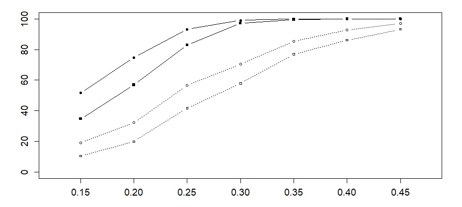
Figure 3: Empirical power of the test based on (20b) with overlapping statistics (dark, solid) and (20a) with non-overlapping statistics (light, dashed) for the level 10% (points) and 5% (squares) under the alternative hypothesis as function of the volatility-jump size Δ​σθ2\Delta\sigma^{2}_{\theta}. The plot gives empirical percentiles exceeding the bootstrapped percentiles under the null hypothesis for hn−1=120h_{n}^{-1}=120, αn=15\alpha_{n}=15 and n=30,000n=30,000.

Figure 3 confirms that the test using (20b) with overlapping statistics has a significantly higher power than the test based on (20a) and non-overlapping statistics. The largest difference for Δ​σθ2=0.2\Delta\sigma^{2}_{\theta}=0.2 is 17.8% at 10% testing level and for Δ​σθ2=0.25\Delta\sigma^{2}_{\theta}=0.25, 14.8% at 5% testing level. Thus, for volatility jumps with moderate absolute size in the range considered in Figure 3, the overlapping statistics attain relevant efficiency gains. The location of the volatility jump – when the boundaries are excluded – does not affect the power of the tests. Figure 3 illustrates increasing power of both tests as Δ​σθ2\Delta\sigma^{2}_{\theta} gets larger. It also reveals that volatility jumps with Δ​σθ2≤0.15\Delta\sigma^{2}_{\theta}\leq 0.15 are difficult to detect in our setting where this corresponds only to approximately 20 times the average absolute increment |Δin​Y||\Delta_{i}^{n}Y|. Due to the required smoothing over blocks we cannot expect to detect such small volatility jumps with good power. We can further report a better accuracy of the theoretical limit law under H0H_{0} from Proposition 4.3 for the empirical distribution of the statistics with overlapping compared to non-overlapping blocks. The average amount of realizations of simulated statistics (20a) exceeding the theoretical 90%-percentile is 9.99% and exceeding the 95%-percentile 6.41%. For the statistics (20b) these values are 21.00% and 11.11%, respectively.

6 Proofs

6.1 Proof of Theorem 4.1

For notational convenience, we replace

maxi=0,…,⌊(αn​hn)−1⌋−2bymaxi,\displaystyle\mathop{\mathrm{max}}\limits_{i=0,\ldots,{\lfloor\left(\alpha_{n}h_{n}\right)^{-1}\rfloor}-2}\quad\text{by}\quad\mathop{\mathrm{max}}\limits_{i},

and

mini=0,…,⌊(αn​hn)−1⌋−2bymini,\displaystyle\mathop{\mathrm{min}}\limits_{i=0,\ldots,{\lfloor\left(\alpha_{n}h_{n}\right)^{-1}\rfloor}-2}\quad\text{by}\quad\mathop{\mathrm{min}}\limits_{i},

respectively.
We also introduce the following notation, adapting the elements of the spectral statistics on each big block. Set

Φi​j​ℓ​(t)\displaystyle\Phi_{ij\ell}\left(t\right) =Φj​(t−(hn​(i​αn+(ℓ−1))))\displaystyle=\Phi_{j}\left(t-\left(h_{n}(i\alpha_{n}+\left(\ell-1\right))\right)\right)

and

φi​j​ℓ​(t)\displaystyle\varphi_{ij\ell}\left(t\right) =φj​(t−(hn​(i​αn+(ℓ−1)))).\displaystyle=\varphi_{j}\left(t-\left(h_{n}(i\alpha_{n}+\left(\ell-1\right))\right)\right)\,.

Furthermore, we define the big block-wise spectral statistics

Si​j​ℓ​(L)=∑ν=1nΔin​Φi​j​ℓ​(νn)\displaystyle S_{ij\ell}\left(L\right)=\sum_{\nu=1}^{n}\Delta_{i}^{n}\Phi_{ij\ell}\left(\frac{\nu}{n}\right)

and the associated variance minimizing oracle weights

wi​j​ℓ=(σhn​(i​αn+(ℓ−1))2+η2n​[φi​j​ℓ,φi​j​ℓ]n)−2∑j=1⌊n​hn⌋−1(σhn​(i​αn+(ℓ−1))2+η2n​[φi​j​ℓ,φi​j​ℓ]n)−2.\displaystyle w_{ij\ell}=\frac{\left(\sigma^{2}_{h_{n}(i\alpha_{n}+\left(\ell-1\right))}+\frac{\eta^{2}}{n}\left[\varphi_{ij\ell},\varphi_{ij\ell}\right]_{n}\right)^{-2}}{\sum_{j=1}^{{\lfloor nh_{n}\rfloor}-1}\left(\sigma^{2}_{h_{n}(i\alpha_{n}+\left(\ell-1\right))}+\frac{\eta^{2}}{n}\left[\varphi_{ij\ell},\varphi_{ij\ell}\right]_{n}\right)^{-2}}\,.

We further introduce the bias correction terms

μi​j​ℓ=[φi​j​ℓ,φi​j​ℓ]n​η2n.\mu_{ij\ell}=[\varphi_{ij\ell},\varphi_{ij\ell}]_{n}\;\frac{\eta^{2}}{n}\,.

We can strengthen the assumptions, presented in Assumption 2.1 and ( H 0 - a ), as follows. We replace local boundedness of (σt)t∈[0,1]\left(\sigma_{t}\right)_{t\in\left[0,1\right]}, (at)t∈[0,1]\left(a_{t}\right)_{t\in\left[0,1\right]}, and the modulus of continuity (wδ​(σ)t)t∈[0,1](w_{\delta}(\sigma)_{t})_{t\in\left[0,1\right]} under ( H 0 - a ) by global boundedness. We refer to Section 4.4.1 of Jacod and Protter (2012) for a proof and the construction through localization. We set

U¯n=maxi=0,…,⌊(αn​hn)−1⌋−2|Z¯n,i−Z¯n,i+1|Z¯n,i+1|3/4|,\displaystyle\overline{U}_{n}=\mathop{\mathrm{max}}\limits_{i=0,\ldots,{\lfloor\left(\alpha_{n}h_{n}\right)^{-1}\rfloor}-2}\left|\frac{\overline{Z}_{n,i}-\overline{Z}_{n,i+1}}{\big|\overline{Z}_{n,i+1}\big|^{3/4}}\right|\,,

with

Z¯n,i:=1αn​∑ℓ=1αn∑j=1⌊n​hn⌋−1wi​j​ℓ​((σi​αn​hn​Si​j​ℓ​(W)+Si​j​ℓ​(ε))2−μi​j​ℓ).\displaystyle\overline{Z}_{n,i}:=\frac{1}{\alpha_{n}}\sum_{\ell=1}^{\alpha_{n}}\sum_{j=1}^{{\lfloor nh_{n}\rfloor}-1}w_{ij\ell}\left(\left(\sigma_{i\alpha_{n}h_{n}}S_{ij\ell}\left(W\right)+S_{ij\ell}\left(\varepsilon\right)\right)^{2}-\mu_{ij\ell}\right). (32)

Finally we fix some constants K+,K−>0K^{+},K^{-}>0, such that almost surely

K−​<inft∈[0,1]σt2andK+>​supt∈[0,1]σt2.\displaystyle K^{-}<\inf_{t\in[0,1]}\sigma^{2}_{t}\quad\text{and}\quad K^{+}>\sup_{t\in[0,1]}\sigma^{2}_{t}\,.

The first step described in Section 4.2 is accomplished in the next proposition.

Proposition 6.1.

Given the assumptions of Theorem 4.1, it holds under ( H 0 - a ) that

αn​log⁡(hn−1)​maxi||R​V¯n,i−R​V¯n,i+1|R​V¯n,i+1|3/4|−|Z¯n,i−Z¯n,i+1|Z¯n,i+1|3/4||​⟶ℙ​0.\displaystyle\sqrt{\alpha_{n}\log\left(h_{n}^{-1}\right)}\mathop{\mathrm{max}}\limits_{i}\left|\bigg|\frac{\overline{RV}_{n,i}-\overline{RV}_{n,i+1}}{\left|\overline{RV}_{n,i+1}\right|^{3/4}}\bigg|-\bigg|\frac{\overline{Z}_{n,i}-\overline{Z}_{n,i+1}}{\left|\overline{Z}_{n,i+1}\right|^{3/4}}\bigg|\right|\overset{\mathbb{P}}{\longrightarrow}0\,.

Proof of Proposition 6.1.
Since hn∝n−1/2log(n)h_{n}\propto n^{-1/2}\log(n) we can proceed as follows. The reverse triangle inequality and the decomposition

R​V¯n,i−R​V¯n,i+1|R​V¯n,i+1|3/4−Z¯n,i−Z¯n,i+1|Z¯n,i+1|3/4\displaystyle\frac{\overline{RV}_{n,i}-\overline{RV}_{n,i+1}}{\left|\overline{RV}_{n,i+1}\right|^{3/4}}-\frac{\overline{Z}_{n,i}-\overline{Z}_{n,i+1}}{\left|\overline{Z}_{n,i+1}\right|^{3/4}}
=R​V¯n,i|R​V¯n,i+1|3/4−R​V¯n,i|Z¯n,i+1|3/4+R​V¯n,i−Z¯n,i|Z¯n,i+1|3/4−R​V¯n,i+1|R​V¯n,i+1|3/4+Z¯n,i+1−R​V¯n,i+1|Z¯n,i+1|3/4\displaystyle=\frac{\overline{RV}_{n,i}}{\left|\overline{RV}_{n,i+1}\right|^{3/4}}-\frac{\overline{RV}_{n,i}}{\left|\overline{Z}_{n,i+1}\right|^{3/4}}+\frac{\overline{RV}_{n,i}-\overline{Z}_{n,i}}{\left|\overline{Z}_{n,i+1}\right|^{3/4}}-\frac{\overline{RV}_{n,i+1}}{\left|\overline{RV}_{n,i+1}\right|^{3/4}}+\frac{\overline{Z}_{n,i+1}-\overline{RV}_{n,i+1}}{\left|\overline{Z}_{n,i+1}\right|^{3/4}}

yield the following decomposition:

maxi|R​V¯n,i​(1|R​V¯n,i+1|3/4−1|Z¯n,i+1|3/4)|+maxi|R​V¯n,i−Z¯n,i|Z¯n,i+1|3/4|\displaystyle\mathop{\mathrm{max}}\limits_{i}\left|\overline{RV}_{n,i}\left(\frac{1}{\left|\overline{RV}_{n,i+1}\right|^{3/4}}-\frac{1}{\left|\overline{Z}_{n,i+1}\right|^{3/4}}\right)\right|+\mathop{\mathrm{max}}\limits_{i}\left|\frac{\overline{RV}_{n,i}-\overline{Z}_{n,i}}{\left|\overline{Z}_{n,i+1}\right|^{3/4}}\right|
+maxi|R​V¯n,i+1(1|Z¯n,i+1|3/4−1|R​V¯n,i+1|3/4)|+maxi|Z¯n,i+1−R​V¯n,i+1|Z¯n,i+1|3/4|\displaystyle\quad+\mathop{\mathrm{max}}\limits_{i}\left|\overline{RV}_{n,i+1}\left(\frac{1}{\left|\overline{Z}_{n,i+1}\right|^{3/4}}-\frac{1}{\big|\overline{RV}_{n,i+1}\big|^{3/4}}\right)\right|+\mathop{\mathrm{max}}\limits_{i}\left|\frac{\overline{Z}_{n,i+1}-\overline{RV}_{n,i+1}}{\left|\overline{Z}_{n,i+1}\right|^{3/4}}\right|
=:(I)+(II)+(III)+(IV).\displaystyle=:\left(\textbf{I}\right)+\left(\textbf{II}\right)+\left(\textbf{III}\right)+\left(\textbf{IV}\right)\,. (33)

Starting with (II)\left(\textbf{II}\right) in (33) we proceed as follows.
For all δ>0\delta>0 and κ−>0\kappa^{-}>0, such that κ−∈(0,K−)\kappa^{-}\in\left(0,K^{-}\right), the following holds:

ℙ[maxi|αn​log⁡(n)​(R​V¯n,i−Z¯n,i)|Z¯n,i+1|3/4|>δ]\displaystyle\mathbb{P}\left[\mathop{\mathrm{max}}\limits_{i}\left|\frac{\sqrt{\alpha_{n}\log\left(n\right)}\left(\overline{RV}_{n,i}-\overline{Z}_{n,i}\right)}{\left|\overline{Z}_{n,i+1}\right|^{3/4}}\right|>\delta\right]
=ℙ[maxi|αn​log⁡(n)​(R​V¯n,i−Z¯n,i)|Z¯n,i+1|3/4|>δ,mini|Z¯n,i+1|≥K−−κ−]\displaystyle=\mathbb{P}\left[\mathop{\mathrm{max}}\limits_{i}\left|\frac{\sqrt{\alpha_{n}\log\left(n\right)}\left(\overline{RV}_{n,i}-\overline{Z}_{n,i}\right)}{\left|\overline{Z}_{n,i+1}\right|^{3/4}}\right|>\delta,\,\mathop{\mathrm{min}}\limits_{i}\left|\overline{Z}_{n,i+1}\right|\geq K^{-}\hskip-6.00006pt-\kappa^{-}\right]
+ℙ[maxi|αn​log⁡(n)​(R​V¯n,i−Z¯n,i)|Z¯n,i+1|3/4|>δ,mini|Z¯n,i+1|<K−−κ−]\displaystyle+\mathbb{P}\left[\mathop{\mathrm{max}}\limits_{i}\left|\frac{\sqrt{\alpha_{n}\log\left(n\right)}\left(\overline{RV}_{n,i}-\overline{Z}_{n,i}\right)}{\left|\overline{Z}_{n,i+1}\right|^{3/4}}\right|>\delta,\,\mathop{\mathrm{min}}\limits_{i}\left|\overline{Z}_{n,i+1}\right|<K^{-}\hskip-6.00006pt-\kappa^{-}\right]
≤ℙ[maxiαn​log⁡(n)|R​V¯n,i−Z¯n,i|>δ(K−−κ−)3/4]+ℙ[mini|Z¯n,i+1|<K−−κ−]\displaystyle\leq\mathbb{P}\left[\mathop{\mathrm{max}}\limits_{i}\sqrt{\alpha_{n}\log\left(n\right)}\left|\overline{RV}_{n,i}-\overline{Z}_{n,i}\right|>\delta\left(K^{-}\hskip-6.00006pt-\kappa^{-}\right)^{3/4}\right]+\mathbb{P}\left[\mathop{\mathrm{min}}\limits_{i}\,\left|\overline{Z}_{n,i+1}\right|<K^{-}\hskip-6.00006pt-\kappa^{-}\right]
=:An+Bn.\displaystyle=:A_{n}+B_{n}. (34)

In (34) we dropped the dependence on the constants δ\delta and K−K^{-} for notational convenience. We start with the term AnA_{n}. We split the term into various summands in the following way:

R​V¯n,i−Z¯n,i=\displaystyle\overline{RV}_{n,i}-\overline{Z}_{n,i}= 1αn​∑ℓ=1αn∑j=1⌊n​hn⌋−1wi​j​ℓ​(Si​j​ℓ2​(X)−σi​αn​hn2​Si​j​ℓ2​(W))\displaystyle\frac{1}{\alpha_{n}}\sum_{\ell=1}^{\alpha_{n}}\sum_{j=1}^{{\lfloor nh_{n}\rfloor}-1}w_{ij\ell}\left(S^{2}_{ij\ell}\left(X\right)-\sigma^{2}_{i\alpha_{n}h_{n}}S^{2}_{ij\ell}\left(W\right)\right)
+2αn∑ℓ=1αn∑j=1⌊n​hn⌋−1wi​j​ℓSi​j​ℓ(ε)(Si​j​ℓ(X)−σi​αn​hnSi​j​ℓ(W)).\displaystyle\quad+\frac{2}{\alpha_{n}}\sum_{\ell=1}^{\alpha_{n}}\sum_{j=1}^{{\lfloor nh_{n}\rfloor}-1}w_{ij\ell}S_{ij\ell}\left(\varepsilon\right)\left(S_{ij\ell}\left(X\right)-\sigma_{i\alpha_{n}h_{n}}S_{ij\ell}\left(W\right)\right).

That yields

An\displaystyle A_{n} ≤ℙ[maxi|log⁡(n)αn∑ℓ=1αn∑j=1⌊n​hn⌋−1wi​j​ℓ(Si​j​ℓ2(X)−σi​αn​hn2Si​j​ℓ2(W))|>δ​(K−−κ−)3/42]\displaystyle\leq\mathbb{P}\left[\mathop{\mathrm{max}}\limits_{i}\left|\frac{\sqrt{\log\left(n\right)}}{\sqrt{\alpha_{n}}}\sum_{\ell=1}^{\alpha_{n}}\sum_{j=1}^{{\lfloor nh_{n}\rfloor}-1}w_{ij\ell}\left(S^{2}_{ij\ell}\left(X\right)-\sigma^{2}_{i\alpha_{n}h_{n}}S^{2}_{ij\ell}\left(W\right)\right)\right|>\frac{\delta\left(K^{-}\hskip-6.00006pt-\kappa^{-}\right)^{3/4}}{2}\right]
+ℙ[maxi|log⁡(n)αn∑ℓ=1αn∑j=1⌊n​hn⌋−1wi​j​ℓSi​j​ℓ(ε)(Si​j​ℓ(X)−σi​αn​hnSi​j​ℓ(W))|>δ​(K−−κ−)3/44]\displaystyle\quad+\mathbb{P}\left[\mathop{\mathrm{max}}\limits_{i}\left|\frac{\sqrt{\log\left(n\right)}}{\sqrt{\alpha_{n}}}\sum_{\ell=1}^{\alpha_{n}}\sum_{j=1}^{{\lfloor nh_{n}\rfloor}-1}w_{ij\ell}S_{ij\ell}\left(\varepsilon\right)\left(S_{ij\ell}\left(X\right)-\sigma_{i\alpha_{n}h_{n}}S_{ij\ell}\left(W\right)\right)\right|>\frac{\delta\left(K^{-}\hskip-6.00006pt-\kappa^{-}\right)^{3/4}}{4}\right]
=:An1+An2.\displaystyle=:A^{1}_{n}+A^{2}_{n}\,. (35)

In order to handle An,1A^{1}_{n,}, we rewrite the spectral statistics Si​j​ℓ​(L)S_{ij\ell}\left(L\right), for any stochastic process (Lt)t∈[0,1]\left(L_{t}\right)_{t\in\left[0,1\right]}, using step functions ξi​j​ℓ(n)\xi^{\left(n\right)}_{ij\ell}, given by

ξi​j​ℓ(n)​(t):\displaystyle\xi^{\left(n\right)}_{ij\ell}\left(t\right): =∑ν=1nΦi​j​ℓ​(νn)​𝟙(ν−1n,νn]​(t)\displaystyle=\sum_{\nu=1}^{n}\Phi_{ij\ell}\left(\frac{\nu}{n}\right)\mathbbm{1}_{\left(\frac{\nu-1}{n},\frac{\nu}{n}\right]}(t)

which yield

Si​j​ℓ​(L)=∫hn​(i​αn+(ℓ−1))−n−1i​αn​hn+ℓ​hnξi​j​ℓ(n)​(s)​d​Ls\displaystyle S_{ij\ell}\left(L\right)=\int_{h_{n}(i\alpha_{n}+\left(\ell-1\right))-n^{-1}}^{i\alpha_{n}h_{n}+\ell h_{n}}\xi^{\left(n\right)}_{ij\ell}\left(s\right)\,dL_{s}

for any semimartingale L=(Lt)t∈[0,1]L=\left(L_{t}\right)_{t\in\left[0,1\right]}.
By virtue of the Itô process structure of (Xt)(X_{t}), we obtain that

∫hn​(i​αn+(ℓ−1))−n−1i​αn​hn+ℓ​hnξi​j​ℓ(n)​(s)​d​Xs=∫hn​(i​αn+(ℓ−1))−n−1i​αn​hn+ℓ​hnξi​j​ℓ(n)​(s)​as​𝑑s+∫hn​(i​αn+(ℓ−1))−n−1i​αn​hn+ℓ​hnξi​j​ℓ(n)​(s)​σs​d​Ws.\displaystyle\int_{h_{n}(i\alpha_{n}+\left(\ell-1\right))-n^{-1}}^{i\alpha_{n}h_{n}+\ell h_{n}}\xi^{\left(n\right)}_{ij\ell}\left(s\right)\,dX_{s}=\int_{h_{n}(i\alpha_{n}+\left(\ell-1\right))-n^{-1}}^{i\alpha_{n}h_{n}+\ell h_{n}}\xi^{\left(n\right)}_{ij\ell}\left(s\right)a_{s}\,ds+\int_{h_{n}(i\alpha_{n}+\left(\ell-1\right))-n^{-1}}^{i\alpha_{n}h_{n}+\ell h_{n}}\xi^{\left(n\right)}_{ij\ell}\left(s\right)\sigma_{s}\,dW_{s}\,.

Itô’s formula yields

Si​j​ℓ2​(X)=\displaystyle S^{2}_{ij\ell}\left(X\right)= 2​∫hn​(i​αn+(ℓ−1))−n−1i​αn​hn+ℓ​hn(X~τ−X~hn​(i​αn+(ℓ−1))−n−1)​ξi​j​ℓ(n)​(τ)​στ​d​Wτ\displaystyle 2\int_{h_{n}(i\alpha_{n}+\left(\ell-1\right))-n^{-1}}^{i\alpha_{n}h_{n}+\ell h_{n}}\left(\widetilde{X}_{\tau}-\widetilde{X}_{h_{n}(i\alpha_{n}+\left(\ell-1\right))-n^{-1}}\right)\xi^{\left(n\right)}_{ij\ell}\left(\tau\right)\sigma_{\tau}\,dW_{\tau}
+2∫hn​(i​αn+(ℓ−1))−n−1i​αn​hn+ℓ​hn(X~τ−X~hn​(i​αn+(ℓ−1))−n−1)ξi​j​ℓ(n)(τ)aτdτ\displaystyle\quad+2\int_{h_{n}(i\alpha_{n}+\left(\ell-1\right))-n^{-1}}^{i\alpha_{n}h_{n}+\ell h_{n}}\left(\widetilde{X}_{\tau}-\widetilde{X}_{h_{n}(i\alpha_{n}+\left(\ell-1\right))-n^{-1}}\right)\xi^{\left(n\right)}_{ij\ell}\left(\tau\right)a_{\tau}\,d\tau
+∫hn​(i​αn+(ℓ−1))−n−1i​αn​hn+ℓ​hn(ξi​j​ℓ(n)(τ))2στ2dτ\displaystyle\quad+\int_{h_{n}(i\alpha_{n}+\left(\ell-1\right))-n^{-1}}^{i\alpha_{n}h_{n}+\ell h_{n}}\left(\xi^{\left(n\right)}_{ij\ell}\left(\tau\right)\right)^{2}\sigma^{2}_{\tau}\,d\tau

with

X~t:=X0+∫0tξi​j​ℓ(n)​(s)​as​𝑑s+∫0tξi​j​ℓ(n)​(s)​σs​d​Ws.\displaystyle\widetilde{X}_{t}:=X_{0}+\int_{0}^{t}\xi^{\left(n\right)}_{ij\ell}\left(s\right)a_{s}\,ds+\int_{0}^{t}\xi^{\left(n\right)}_{ij\ell}\left(s\right)\sigma_{s}\,dW_{s}.

Similarly,

Si​j​ℓ2​(W)=2​∫hn​(i​αn+(ℓ−1))−n−1i​αn​hn+ℓ​hnW~τ​ξi​j​ℓ(n)​(τ)​d​Wτ+∫hn​(i​αn+(ℓ−1))−n−1i​αn​hn+ℓ​hn(ξi​j​ℓ(n)​(τ))2​𝑑τ\displaystyle S^{2}_{ij\ell}\left(W\right)=2\int_{h_{n}(i\alpha_{n}+\left(\ell-1\right))-n^{-1}}^{i\alpha_{n}h_{n}+\ell h_{n}}\widetilde{W}_{\tau}\,\xi^{\left(n\right)}_{ij\ell}\left(\tau\right)\,dW_{\tau}+\int_{h_{n}(i\alpha_{n}+\left(\ell-1\right))-n^{-1}}^{i\alpha_{n}h_{n}+\ell h_{n}}\left(\xi^{\left(n\right)}_{ij\ell}\left(\tau\right)\right)^{2}\,d\tau

with

W~t:=∫0tξi​j​ℓ(n)​(s)​d​Ws.\displaystyle\widetilde{W}_{t}:=\int_{0}^{t}\xi^{\left(n\right)}_{ij\ell}\left(s\right)\,dW_{s}\,.

For notational brevity, we suppress the dependence of X~t\widetilde{X}_{t} and W~t\widetilde{W}_{t}, respectively, on (i,j,ℓ,n)\left(i,j,\ell,n\right). We bound An1A_{n}^{1} via

An1≤An1,1+An1,2+An1,3,\displaystyle A^{1}_{n}\leq A^{1,1}_{n}+A^{1,2}_{n}+A^{1,3}_{n}\,,

where

An1,1\displaystyle A^{1,1}_{n} =ℙ[maxi|log⁡(n)αn∑ℓ=1αn∑j=1⌊n​hn⌋−1wi​j​ℓ∫hn​(i​αn+(ℓ−1))−n−1i​αn​hn+ℓ​hn(X~τ−X~hn​(i​αn+(ℓ−1))−n−1)\displaystyle=\mathbb{P}\bigg[\mathop{\mathrm{max}}\limits_{i}\bigg|\frac{\sqrt{\log\left(n\right)}}{\sqrt{\alpha_{n}}}\sum_{\ell=1}^{\alpha_{n}}\sum_{j=1}^{{\lfloor nh_{n}\rfloor}-1}w_{ij\ell}\int_{h_{n}(i\alpha_{n}+\left(\ell-1\right))-n^{-1}}^{i\alpha_{n}h_{n}+\ell h_{n}}\left(\widetilde{X}_{\tau}-\widetilde{X}_{h_{n}(i\alpha_{n}+\left(\ell-1\right))-n^{-1}}\right)
×ξi​j​ℓ(n)(τ)aτdτ|>δ​(K−−κ−)3/412],\displaystyle\hskip 170.71652pt\times\xi^{\left(n\right)}_{ij\ell}\left(\tau\right)a_{\tau}\,d\tau\bigg|>\frac{\delta\left(K^{-}\hskip-6.00006pt-\kappa^{-}\right)^{3/4}}{12}\bigg]\,,
An1,2=ℙ[maxi|log⁡(n)αn∑ℓ=1αn∑j=1⌊n​hn⌋−1wi​j​ℓ∫hn​(i​αn+(ℓ−1))−n−1i​αn​hn+ℓ​hn(ξi​j​ℓ(n)(τ))2\displaystyle A_{n}^{1,2}=\mathbb{P}\Bigg[\mathop{\mathrm{max}}\limits_{i}\bigg|\frac{\sqrt{\log\left(n\right)}}{\sqrt{\alpha_{n}}}\sum_{\ell=1}^{\alpha_{n}}\sum_{j=1}^{{\lfloor nh_{n}\rfloor}-1}w_{ij\ell}\int_{h_{n}(i\alpha_{n}+\left(\ell-1\right))-n^{-1}}^{i\alpha_{n}h_{n}+\ell h_{n}}\left(\xi^{\left(n\right)}_{ij\ell}\left(\tau\right)\right)^{2}
×(στ2−σi​αn​hn2)dτ|>δ​(K−−κ−)3/46],\displaystyle\hskip 113.81102pt\times\left(\sigma^{2}_{\tau}-\sigma^{2}_{i\alpha_{n}h_{n}}\right)\,d\tau\bigg|>\frac{\delta\left(K^{-}\hskip-6.00006pt-\kappa^{-}\right)^{3/4}}{6}\Bigg]\,,

and

An1,3\displaystyle A_{n}^{1,3} =ℙ[maxi|log⁡(n)αn∑ℓ=1αn∑j=1⌊n​hn⌋−1wi​j​ℓ∫hn​(i​αn+(ℓ−1))−n−1i​αn​hn+ℓ​hnξi​j​ℓ(n)(τ)\displaystyle=\mathbb{P}\left[\mathop{\mathrm{max}}\limits_{i}\left|\frac{\sqrt{\log\left(n\right)}}{\sqrt{\alpha_{n}}}\sum_{\ell=1}^{\alpha_{n}}\sum_{j=1}^{{\lfloor nh_{n}\rfloor}-1}w_{ij\ell}\int_{h_{n}(i\alpha_{n}+\left(\ell-1\right))-n^{-1}}^{i\alpha_{n}h_{n}+\ell h_{n}}\xi^{\left(n\right)}_{ij\ell}\left(\tau\right)\right.\right.
×((X~τ−X~hn​(i​αn+(ℓ−1))−n−1)στ−σi​αn​hn2W~τ)dWτ|>δ​(K−−κ−)3/412].\displaystyle\quad\left.\left.{\vphantom{\mathop{\mathrm{max}}\limits_{i}\frac{\sqrt{\log\left(n\right)}}{\sqrt{\alpha_{n}}}\sum_{\ell=1}^{\alpha_{n}}}}\times\left(\left(\widetilde{X}_{\tau}-\widetilde{X}_{h_{n}(i\alpha_{n}+\left(\ell-1\right))-n^{-1}}\right)\sigma_{\tau}-\sigma^{2}_{i\alpha_{n}h_{n}}\widetilde{W}_{\tau}\right)dW_{\tau}\right|>\frac{\delta\left(K^{-}\hskip-6.00006pt-\kappa^{-}\right)^{3/4}}{12}\right]\,.

Starting with An1,1A_{n}^{1,1} we employ Markov’s inequality, applied to the function z↦|z|rz\mapsto\left|z\right|^{r}, r>0r>0 and r∈ℕr\in\mathbb{N}:

ℙ[|log⁡(n)αn∑ℓ=1αn∑j=1⌊n​hn⌋−1wi​j​ℓ∫hn​(i​αn+(ℓ−1))−n−1i​αn​hn+ℓ​hn(X~τ−X~hn​(i​αn+(ℓ−1))−n−1)ξi​j​ℓ(n)(τ)aτdτ|>δ​(K−−κ−)3/412]\displaystyle\mathbb{P}\hskip-1.42271pt\bigg[\bigg|\frac{\sqrt{\log\left(n\right)}}{\sqrt{\alpha_{n}}}\hskip-1.42271pt\sum_{\ell=1}^{\alpha_{n}}\hskip-2.84544pt\sum_{j=1}^{{\lfloor nh_{n}\rfloor}-1}\hskip-5.69046ptw_{ij\ell}\hskip-1.42271pt\int_{h_{n}(i\alpha_{n}+\left(\ell-1\right))-n^{-1}}^{i\alpha_{n}h_{n}+\ell h_{n}}\hskip-2.84544pt\left(\widetilde{X}_{\tau}\hskip-1.42271pt-\hskip-1.42271pt\widetilde{X}_{h_{n}(i\alpha_{n}+\left(\ell-1\right))-n^{-1}}\right)\xi^{\left(n\right)}_{ij\ell}\hskip-1.42271pt\left(\tau\right)a_{\tau}\,d\tau\bigg|>\frac{\delta(K^{-}\hskip-6.00006pt-\kappa^{-})^{3/4}}{12}\bigg]
≤(12δ​(K−−κ−)3/4)r(log(n))r/2αn−r/2\displaystyle\leq\left(\frac{12}{\delta\left(K^{-}\hskip-6.00006pt-\kappa^{-}\right)^{3/4}}\right)^{r}\left(\log\left(n\right)\right)^{r/2}\alpha_{n}^{-r/2}
×𝔼⁡[|∑ℓ=1αn∑j=1⌊n​hn⌋−1wi​j​ℓ​∫hn​(i​αn+(ℓ−1))−n−1i​αn​hn+ℓ​hn(X~τ−X~hn​(i​αn+(ℓ−1))−n−1)​ξi​j​ℓ(n)​(τ)​aτ​𝑑τ|r].\displaystyle\quad\quad\quad\times\mathbb{E}\left[\left|\sum_{\ell=1}^{\alpha_{n}}\sum_{j=1}^{{\lfloor nh_{n}\rfloor}-1}w_{ij\ell}\int_{h_{n}(i\alpha_{n}+\left(\ell-1\right))-n^{-1}}^{i\alpha_{n}h_{n}+\ell h_{n}}\left(\widetilde{X}_{\tau}-\widetilde{X}_{h_{n}(i\alpha_{n}+\left(\ell-1\right))-n^{-1}}\right)\xi^{\left(n\right)}_{ij\ell}\left(\tau\right)a_{\tau}\,d\tau\right|^{r}\right].

The identity

𝔼⁡[|∑ℓ=1αn∑j=1⌊n​hn⌋−1wi​j​ℓ​∫hn​(i​αn+(ℓ−1))−n−1i​αn​hn+ℓ​hn(X~τ−X~hn​(i​αn+(ℓ−1))−n−1)​ξi​j​ℓ(n)​(τ)​aτ​𝑑τ|r]\displaystyle\mathbb{E}\left[\left|\sum_{\ell=1}^{\alpha_{n}}\sum_{j=1}^{{\lfloor nh_{n}\rfloor}-1}w_{ij\ell}\int_{h_{n}(i\alpha_{n}+\left(\ell-1\right))-n^{-1}}^{i\alpha_{n}h_{n}+\ell h_{n}}\left(\widetilde{X}_{\tau}-\widetilde{X}_{h_{n}(i\alpha_{n}+\left(\ell-1\right))-n^{-1}}\right)\xi^{\left(n\right)}_{ij\ell}\left(\tau\right)a_{\tau}\,d\tau\right|^{r}\right]
=αnr​𝔼​[|∑ℓ=1αn1αn​∑j=1⌊n​hn⌋−1wi​j​ℓ​∫hn​(i​αn+(ℓ−1))−n−1i​αn​hn+ℓ​hn(X~τ−X~hn​(i​αn+(ℓ−1))−n−1)​ξi​j​ℓ(n)​(τ)​aτ​𝑑τ|r]\displaystyle=\alpha_{n}^{r}\,\mathbb{E}\left[\left|\sum_{\ell=1}^{\alpha_{n}}\frac{1}{\alpha_{n}}\sum_{j=1}^{{\lfloor nh_{n}\rfloor}-1}w_{ij\ell}\int_{h_{n}(i\alpha_{n}+\left(\ell-1\right))-n^{-1}}^{i\alpha_{n}h_{n}+\ell h_{n}}\left(\widetilde{X}_{\tau}-\widetilde{X}_{h_{n}(i\alpha_{n}+\left(\ell-1\right))-n^{-1}}\right)\xi^{\left(n\right)}_{ij\ell}\left(\tau\right)a_{\tau}\,d\tau\right|^{r}\right]

implies, together with Jensen’s inequality, that

αnr/2​𝔼​[|∑ℓ=1αn1αn​∑j=1⌊n​hn⌋−1wi​j​ℓ​∫hn​(i​αn+(ℓ−1))−n−1i​αn​hn+ℓ​hn(X~τ−X~hn​(i​αn+(ℓ−1))−n−1)​ξi​j​ℓ(n)​(τ)​aτ​𝑑τ|r]\displaystyle\alpha_{n}^{r/2}\mathbb{E}\left[\left|\sum_{\ell=1}^{\alpha_{n}}\frac{1}{\alpha_{n}}\sum_{j=1}^{{\lfloor nh_{n}\rfloor}-1}w_{ij\ell}\int_{h_{n}(i\alpha_{n}+\left(\ell-1\right))-n^{-1}}^{i\alpha_{n}h_{n}+\ell h_{n}}\left(\widetilde{X}_{\tau}-\widetilde{X}_{h_{n}(i\alpha_{n}+\left(\ell-1\right))-n^{-1}}\right)\xi^{\left(n\right)}_{ij\ell}\left(\tau\right)a_{\tau}\,d\tau\right|^{r}\right]
≤αnr/2−1​∑ℓ=1αn𝔼⁡[|∑j=1⌊n​hn⌋−1wi​j​ℓ​∫hn​(i​αn+(ℓ−1))−n−1i​αn​hn+ℓ​hn(X~τ−X~hn​(i​αn+(ℓ−1))−n−1)​ξi​j​ℓ(n)​(τ)​aτ​𝑑τ|r]\displaystyle\leq\alpha_{n}^{r/2-1}\sum_{\ell=1}^{\alpha_{n}}\mathbb{E}\left[\left|\sum_{j=1}^{{\lfloor nh_{n}\rfloor}-1}w_{ij\ell}\int_{h_{n}(i\alpha_{n}+\left(\ell-1\right))-n^{-1}}^{i\alpha_{n}h_{n}+\ell h_{n}}\left(\widetilde{X}_{\tau}-\widetilde{X}_{h_{n}(i\alpha_{n}+\left(\ell-1\right))-n^{-1}}\right)\xi^{\left(n\right)}_{ij\ell}\left(\tau\right)a_{\tau}\,d\tau\right|^{r}\right]
≤αnr/2−1​∑ℓ=1αn∑j=1⌊n​hn⌋−1wi​j​ℓ​𝔼​[|∫hn​(i​αn+(ℓ−1))−n−1i​αn​hn+ℓ​hn(X~τ−X~hn​(i​αn+(ℓ−1))−n−1)​ξi​j​ℓ(n)​(τ)​aτ​𝑑τ|r].\displaystyle\leq\alpha_{n}^{r/2-1}\sum_{\ell=1}^{\alpha_{n}}\sum_{j=1}^{{\lfloor nh_{n}\rfloor}-1}w_{ij\ell}\mathbb{E}\left[\left|\int_{h_{n}(i\alpha_{n}+\left(\ell-1\right))-n^{-1}}^{i\alpha_{n}h_{n}+\ell h_{n}}\left(\widetilde{X}_{\tau}-\widetilde{X}_{h_{n}(i\alpha_{n}+\left(\ell-1\right))-n^{-1}}\right)\xi^{\left(n\right)}_{ij\ell}\left(\tau\right)a_{\tau}\,d\tau\right|^{r}\right].

Concerning the second inequality we have taken into account, that ∑jwi​j​ℓ=1\sum_{j}w_{ij\ell}=1 in order to apply Jensen’s inequality a second time.
We employ the generalized Minkowski inequality for double measure integrals, which implies

𝔼⁡[|∫hn​(i​αn+(ℓ−1))−n−1i​αn​hn+ℓ​hn(X~τ−X~hn​(i​αn+(ℓ−1))−n−1)​ξi​j​ℓ(n)​(τ)​aτ​𝑑τ|r]\displaystyle\mathbb{E}\left[\left|\int_{h_{n}(i\alpha_{n}+\left(\ell-1\right))-n^{-1}}^{i\alpha_{n}h_{n}+\ell h_{n}}\left(\widetilde{X}_{\tau}-\widetilde{X}_{h_{n}(i\alpha_{n}+\left(\ell-1\right))-n^{-1}}\right)\xi^{\left(n\right)}_{ij\ell}\left(\tau\right)a_{\tau}\,d\tau\right|^{r}\right]
≤\displaystyle\leq (∫hn​(i​αn+(ℓ−1))−n−1i​αn​hn+ℓ​hn𝔼​[|(X~τ−X~hn​(i​αn+(ℓ−1))−n−1)​ξi​j​ℓ(n)​(τ)​aτ|r]1/r​𝑑τ)r.\displaystyle\left(\int_{h_{n}(i\alpha_{n}+\left(\ell-1\right))-n^{-1}}^{i\alpha_{n}h_{n}+\ell h_{n}}\mathbb{E}\left[\left|\left(\widetilde{X}_{\tau}-\widetilde{X}_{h_{n}(i\alpha_{n}+\left(\ell-1\right))-n^{-1}}\right)\xi^{\left(n\right)}_{ij\ell}\left(\tau\right)a_{\tau}\right|^{r}\right]^{1/r}\,d\tau\right)^{r}\,. (36)

In order to bound the expectation in (36), we apply Burkolder’s inequality to the local martingale part. The general case can be handled via the elementary inequality |a+b|p≤2p​(|a|p+|b|p)\left|a+b\right|^{p}\leq 2^{p}\left(\left|a\right|^{p}+\left|b\right|^{p}\right) and the standard bound for Lebesgue integrals

∫Ωf⁡(s)​𝑑μ​(s)≤μ⁡(Ω)​sups|f⁡(s)|,\displaystyle\int_{\Omega}f(s)\,d\mu(s)\leq\mu\left(\Omega\right)\sup_{s}\left|f(s)\right|\,, (37)

applied to the finite variation part. Taking into account, that the quadratic variation process, ([X~,X~]t)t∈[0,1]\big([\widetilde{X},\widetilde{X}]_{t}\big)_{t\in[0,1]}, is given by

[X~,X~]t=∫0t(ξi​j​ℓ(n)​(s))2​σs2​𝑑s.\displaystyle[\widetilde{X},\widetilde{X}]_{t}=\int_{0}^{t}\left(\xi^{\left(n\right)}_{ij\ell}\left(s\right)\right)^{2}\sigma^{2}_{s}\,ds.

yields

𝔼⁡[|X~τ−X~hn​(i​αn+(ℓ−1))−n−1|r]≤\displaystyle\mathbb{E}\left[\left|\widetilde{X}_{\tau}-\widetilde{X}_{h_{n}(i\alpha_{n}+\left(\ell-1\right))-n^{-1}}\right|^{r}\right]\leq Cr​𝔼​[(∫hn​(i​αn+(ℓ−1))−n−1τ(ξi​j​ℓ(n)​(s))2​σs2​𝑑s)r/2]\displaystyle C_{r}\mathbb{E}\left[\left(\int_{h_{n}(i\alpha_{n}+\left(\ell-1\right))-n^{-1}}^{\tau}\left(\xi^{\left(n\right)}_{ij\ell}\left(s\right)\right)^{2}\sigma^{2}_{s}\,ds\right)^{r/2}\right]
≤\displaystyle\leq Cr​𝔼​[(∫hn​(i​αn+(ℓ−1))−n−1i​αn​hn+ℓ​hn(ξi​j​ℓ(n)​(s))2​σs2​𝑑s)r/2]\displaystyle C_{r}\mathbb{E}\left[\left(\int_{h_{n}(i\alpha_{n}+\left(\ell-1\right))-n^{-1}}^{i\alpha_{n}h_{n}+\ell h_{n}}\left(\xi^{\left(n\right)}_{ij\ell}\left(s\right)\right)^{2}\sigma^{2}_{s}\,ds\right)^{r/2}\right]
≤\displaystyle\leq Crhnr/2hn−r/2=𝒪(1).\displaystyle C_{r}h_{n}^{r/2}h_{n}^{-r/2}=\mathcal{O}(1)\,. (38)

(38) is a consequence of (37),

ξi​j​ℓ(n)​(x)=𝒪⁡(1hn),\displaystyle\xi^{\left(n\right)}_{ij\ell}\left(x\right)=\mathcal{O}\left(\frac{1}{\sqrt{h_{n}}}\right)\,, (39)

and the global boundedness of (σt2)t∈[0,1]\left(\sigma^{2}_{t}\right)_{t\in\left[0,1\right]}. Consequently the above yields

(log⁡(n))r/2αn1−r/2​∑ℓ=1αn∑j=1⌊n​hn⌋−1wi​j​ℓ​𝔼​[|∫hn​(i​αn+(ℓ−1))−n−1i​αn​hn+ℓ​hn(X~τ−X~hn​(i​αn+(ℓ−1))−n−1)​ξi​j​ℓ(n)​(τ)​aτ​𝑑τ|r]\displaystyle\frac{\left(\log\left(n\right)\right)^{r/2}}{\alpha_{n}^{1-r/2}}\sum_{\ell=1}^{\alpha_{n}}\sum_{j=1}^{{\lfloor nh_{n}\rfloor}-1}\hskip-4.26773ptw_{ij\ell}\mathbb{E}\left[\left|\int_{h_{n}(i\alpha_{n}+\left(\ell-1\right))-n^{-1}}^{i\alpha_{n}h_{n}+\ell h_{n}}\left(\widetilde{X}_{\tau}\hskip-1.42271pt-\hskip-1.42271pt\widetilde{X}_{h_{n}(i\alpha_{n}+\left(\ell-1\right))-n^{-1}}\hskip-1.42271pt\right)\xi^{\left(n\right)}_{ij\ell}\left(\tau\right)a_{\tau}\,d\tau\right|^{r}\right]
≤(log(n))r/2αnr/2−1∑ℓ=1αn∑j=1⌊n​hn⌋−1wi​j​ℓhnrhn−r/2=𝒪(log(n)r/2αnr/2hnr/2).\displaystyle\leq\left(\log\left(n\right)\right)^{r/2}\alpha_{n}^{r/2-1}\sum_{\ell=1}^{\alpha_{n}}\sum_{j=1}^{{\lfloor nh_{n}\rfloor}-1}w_{ij\ell}h^{r}_{n}h^{-r/2}_{n}=\mathcal{O}\left(\log\left(n\right)^{r/2}\alpha_{n}^{r/2}h^{r/2}_{n}\right)\,.

Taking into account that

αn​hn=𝒪⁡(n−14​𝔞+2​(log⁡(n))1−2​𝔞2​𝔞+1),\displaystyle\alpha_{n}h_{n}=\mathcal{O}\left(n^{-\frac{1}{4\mathfrak{a}+2}}\left(\log\left(n\right)\right)^{1-\frac{2\mathfrak{a}}{2\mathfrak{a}+1}}\right)\,,

we can conclude, if r>2r>2, that

An1,1\displaystyle A^{1,1}_{n} =𝒪⁡((αn​hn)−1​log⁡(n)r/2​αnr/2​hnr/2)=𝒪⁡(1), as ​n→∞.\displaystyle=\mathcal{O}\left(\left(\alpha_{n}h_{n}\right)^{-1}\log\left(n\right)^{r/2}\alpha_{n}^{r/2}h^{r/2}_{n}\right)={\scriptstyle{\mathcal{O}}}\left(1\right)\,,\text{ as }n\rightarrow\infty\,.

For the term An1,2A^{1,2}_{n}, we start with

log⁡(n)αn​|∑ℓ=1αn∑j=1⌊n​hn⌋−1wi​j​ℓ​∫hn​(i​αn+(ℓ−1))−n−1i​αn​hn+ℓ​hn(ξi​j​ℓ(n)​(τ))2​(στ2−σi​αn​hn2)​𝑑τ|\displaystyle\frac{\sqrt{\log\left(n\right)}}{\sqrt{\alpha_{n}}}\left|\sum_{\ell=1}^{\alpha_{n}}\sum_{j=1}^{{\lfloor nh_{n}\rfloor}-1}w_{ij\ell}\int_{h_{n}(i\alpha_{n}+\left(\ell-1\right))-n^{-1}}^{i\alpha_{n}h_{n}+\ell h_{n}}\left(\xi^{\left(n\right)}_{ij\ell}\left(\tau\right)\right)^{2}\left(\sigma^{2}_{\tau}-\sigma^{2}_{i\alpha_{n}h_{n}}\right)\,d\tau\right|
≤log⁡(n)αn​∑ℓ=1αn∑j=1⌊n​hn⌋−1wi​j​ℓ​∫hn​(i​αn+(ℓ−1))−n−1i​αn​hn+ℓ​hn(ξi​j​ℓ(n)​(τ))2​|στ2−σi​αn​hn2|​𝑑τ.\displaystyle\leq\frac{\sqrt{\log\left(n\right)}}{\sqrt{\alpha_{n}}}\sum_{\ell=1}^{\alpha_{n}}\sum_{j=1}^{{\lfloor nh_{n}\rfloor}-1}w_{ij\ell}\int_{h_{n}(i\alpha_{n}+\left(\ell-1\right))-n^{-1}}^{i\alpha_{n}h_{n}+\ell h_{n}}\left(\xi^{\left(n\right)}_{ij\ell}\left(\tau\right)\right)^{2}\left|\sigma^{2}_{\tau}-\sigma^{2}_{i\alpha_{n}h_{n}}\right|\,d\tau\,. (40)

In (40) the triangle inequality and Jensen’s inequality are applied. Combining the regularity under ( H 0 - a ) and (13) gives

log⁡(n)αn​∑ℓ=1αn∑j=1⌊n​hn⌋−1wi​j​ℓ​∫hn​(i​αn+(ℓ−1))−n−1i​αn​hn+ℓ​hn(ξi​j​ℓ(n)​(τ))2​|στ2−σi​αn​hn2|​𝑑τ\displaystyle\frac{\sqrt{\log\left(n\right)}}{\sqrt{\alpha_{n}}}\sum_{\ell=1}^{\alpha_{n}}\sum_{j=1}^{{\lfloor nh_{n}\rfloor}-1}w_{ij\ell}\int_{h_{n}(i\alpha_{n}+\left(\ell-1\right))-n^{-1}}^{i\alpha_{n}h_{n}+\ell h_{n}}\left(\xi^{\left(n\right)}_{ij\ell}\left(\tau\right)\right)^{2}\left|\sigma^{2}_{\tau}-\sigma^{2}_{i\alpha_{n}h_{n}}\right|\,d\tau
=𝒪ℙ​(log⁡(n)​αn​(αn​hn)𝔞),uniformly in i\displaystyle=\mathcal{O}_{\mathbb{P}}\left(\sqrt{\log\left(n\right)}\sqrt{\alpha_{n}}\left(\alpha_{n}h_{n}\right)^{\mathfrak{a}}\right)\,,\,\text{uniformly in $i$}
=𝒪⁡(1), as ​n→∞.\displaystyle={\scriptstyle{\mathcal{O}}}\left(1\right)\,,\text{ as }n\rightarrow\infty.

Concerning An1,3A^{1,3}_{n} we use further decompositions rewriting

(X~τ−X~hn​(i​αn+(ℓ−1))−n−1)​στ−W~τ​σi​αn​hn2\displaystyle\left(\widetilde{X}_{\tau}-\widetilde{X}_{h_{n}(i\alpha_{n}+\left(\ell-1\right))-n^{-1}}\right)\sigma_{\tau}-\widetilde{W}_{\tau}\sigma^{2}_{i\alpha_{n}h_{n}} (41)

in the following way:

(X~τ−X~hn​(i​αn+(ℓ−1))−n−1)​στ−W~τ​σi​αn​hn2\displaystyle\left(\widetilde{X}_{\tau}-\widetilde{X}_{h_{n}(i\alpha_{n}+\left(\ell-1\right))-n^{-1}}\right)\sigma_{\tau}-\widetilde{W}_{\tau}\sigma^{2}_{i\alpha_{n}h_{n}}
=στ​∫hn​(i​αn+(ℓ−1))−n−1τξi​j​ℓ(n)​(s)​as​𝑑s\displaystyle=\sigma_{\tau}\int_{h_{n}(i\alpha_{n}+\left(\ell-1\right))-n^{-1}}^{\tau}\xi^{\left(n\right)}_{ij\ell}\left(s\right)a_{s}\,ds
+στ∫hn​(i​αn+(ℓ−1))−n−1τξi​j​ℓ(n)(s)σsdWs−σi​αn​hn∫hn​(i​αn+(ℓ−1))−n−1τξi​j​ℓ(n)(s)σsdWs\displaystyle+\sigma_{\tau}\int_{h_{n}(i\alpha_{n}+\left(\ell-1\right))-n^{-1}}^{\tau}\xi^{\left(n\right)}_{ij\ell}\left(s\right)\sigma_{s}\,dW_{s}-\sigma_{i\alpha_{n}h_{n}}\int_{h_{n}(i\alpha_{n}+\left(\ell-1\right))-n^{-1}}^{\tau}\xi^{\left(n\right)}_{ij\ell}\left(s\right)\sigma_{s}\,dW_{s}
+σi​αn​hn∫hn​(i​αn+(ℓ−1))−n−1τξi​j​ℓ(n)(s)σsdWs−σi​αn​hn∫hn​(i​αn+(ℓ−1))−n−1τξi​j​ℓ(n)(s)σi​αn​hndWs\displaystyle+\sigma_{i\alpha_{n}h_{n}}\int_{h_{n}(i\alpha_{n}+\left(\ell-1\right))-n^{-1}}^{\tau}\xi^{\left(n\right)}_{ij\ell}\left(s\right)\sigma_{s}\,dW_{s}-\sigma_{i\alpha_{n}h_{n}}\int_{h_{n}(i\alpha_{n}+\left(\ell-1\right))-n^{-1}}^{\tau}\xi^{\left(n\right)}_{ij\ell}\left(s\right)\sigma_{i\alpha_{n}h_{n}}\,dW_{s}
=στ​∫hn​(i​αn+(ℓ−1))−n−1τξi​j​ℓ(n)​(s)​as​𝑑s\displaystyle=\sigma_{\tau}\int_{h_{n}(i\alpha_{n}+\left(\ell-1\right))-n^{-1}}^{\tau}\xi^{\left(n\right)}_{ij\ell}\left(s\right)a_{s}\,ds (42)
+(στ−σi​αn​hn)∫hn​(i​αn+(ℓ−1))−n−1τξi​j​ℓ(n)(s)σsdWs\displaystyle+\left(\sigma_{\tau}-\sigma_{i\alpha_{n}h_{n}}\right)\int_{h_{n}(i\alpha_{n}+\left(\ell-1\right))-n^{-1}}^{\tau}\xi^{\left(n\right)}_{ij\ell}\left(s\right)\sigma_{s}\,dW_{s} (43)
+σi​αn​hn∫hn​(i​αn+(ℓ−1))−n−1τξi​j​ℓ(n)(s)(σs−σi​αn​hn)dWs.\displaystyle+\sigma_{i\alpha_{n}h_{n}}\int_{h_{n}(i\alpha_{n}+\left(\ell-1\right))-n^{-1}}^{\tau}\xi^{\left(n\right)}_{ij\ell}\left(s\right)\left(\sigma_{s}-\sigma_{i\alpha_{n}h_{n}}\right)\,dW_{s}\,. (44)

Using this decomposition, we can bound An1,3A_{n}^{1,3} via

An1,3≤An1,3​a+An1,3​b+An1,3​c.\displaystyle A_{n}^{1,3}\leq A_{n}^{1,3a}+A_{n}^{1,3b}+A_{n}^{1,3c}\,.

We start with the probability involving the summand (42). We have to bound the probability

ℙ[|log⁡(n)αn∑ℓ=1αn∑j=1⌊n​hn⌋−1∫hn​(i​αn+(ℓ−1))−n−1i​αn​hn+ℓ​hnwi​j​ℓξi​j​ℓ(n)(τ)στ\displaystyle\mathbb{P}\left[\left|\frac{\sqrt{\log\left(n\right)}}{\sqrt{\alpha_{n}}}\sum_{\ell=1}^{\alpha_{n}}\sum_{j=1}^{{\lfloor nh_{n}\rfloor}-1}\int_{h_{n}(i\alpha_{n}+\left(\ell-1\right))-n^{-1}}^{i\alpha_{n}h_{n}+\ell h_{n}}w_{ij\ell}\xi^{\left(n\right)}_{ij\ell}\left(\tau\right)\sigma_{\tau}\right.\right.
×∫hn​(i​αn+(ℓ−1))−n−1τξi​j​ℓ(n)(s)asdsdWτ|>δ​(K−−κ−)3/436]\displaystyle\left.\left.\hskip 113.81102pt\quad\quad\times\int_{h_{n}(i\alpha_{n}+\left(\ell-1\right))-n^{-1}}^{\tau}\xi^{\left(n\right)}_{ij\ell}\left(s\right)a_{s}\,ds\,dW_{\tau}\right|>\frac{\delta\left(K^{-}\hskip-6.00006pt-\kappa^{-}\right)^{3/4}}{36}\right]
≤(36δ​(K−−κ−)3/4)r​(log⁡(n)αn)r\displaystyle\leq\left(\frac{36}{\delta\left(K^{-}\hskip-6.00006pt-\kappa^{-}\right)^{3/4}}\right)^{r}\left(\frac{\sqrt{\log\left(n\right)}}{\sqrt{\alpha_{n}}}\right)^{r}
×𝔼⁡[|∑ℓ=1αn∑j=1⌊n​hn⌋−1wi​j​ℓ​∫hn​(i​αn+(ℓ−1))−n−1i​αn​hn+ℓ​hnξi​j​ℓ(n)​(τ)​στ​∫hn​(i​αn+(ℓ−1))−n−1τξi​j​ℓ(n)​(s)​as​𝑑s​d​Wτ|r],\displaystyle\quad\times\mathbb{E}\left[\left|\sum_{\ell=1}^{\alpha_{n}}\sum_{j=1}^{{\lfloor nh_{n}\rfloor}-1}w_{ij\ell}\int_{h_{n}(i\alpha_{n}+\left(\ell-1\right))-n^{-1}}^{i\alpha_{n}h_{n}+\ell h_{n}}\xi^{\left(n\right)}_{ij\ell}\left(\tau\right)\sigma_{\tau}\int_{h_{n}(i\alpha_{n}+\left(\ell-1\right))-n^{-1}}^{\tau}\xi^{\left(n\right)}_{ij\ell}\left(s\right)a_{s}\,ds\,dW_{\tau}\right|^{r}\right]\,,

where we have applied Markov’s inequality with some exponent r>0r>0 and r∈ℕr\in\mathbb{N}. Set

cn,i​(τ)=∑ℓ=1αnστ​∑j=1⌊n​hn⌋−1wi​j​ℓ​ξi​j​ℓ(n)​(τ)​∫hn​(i​αn+(ℓ−1))−n−1τξi​j​ℓ(n)​(s)​as​𝑑s\displaystyle c_{n,i}\left(\tau\right)=\sum_{\ell=1}^{\alpha_{n}}\sigma_{\tau}\sum_{j=1}^{{\lfloor nh_{n}\rfloor}-1}w_{ij\ell}\xi^{\left(n\right)}_{ij\ell}\left(\tau\right)\int_{h_{n}(i\alpha_{n}+\left(\ell-1\right))-n^{-1}}^{\tau}\xi^{\left(n\right)}_{ij\ell}\left(s\right)a_{s}\,ds
×𝟙(hn(iαn+(ℓ−1))−n−1,iαnhn+ℓhn](τ).\displaystyle\times\mathbbm{1}_{\left(h_{n}(i\alpha_{n}+\left(\ell-1\right))-n^{-1},i\alpha_{n}h_{n}+\ell h_{n}\right]}\left(\tau\right)\,.

In order to apply Itô isometry, we set r=2​mr=2m, with some m>0m>0 and m∈ℕm\in\mathbb{N}. We derive that

𝔼⁡[|∑ℓ=1αn∑j=1⌊n​hn⌋−1wi​j​ℓ​∫hn​(i​αn+(ℓ−1))−n−1i​αn​hn+ℓ​hnξi​j​ℓ(n)​(τ)​στ​∫hn​(i​αn+(ℓ−1))−n−1τξi​j​ℓ(n)​(s)​as​𝑑s​d​Wτ|r]\displaystyle\mathbb{E}\left[\left|\sum_{\ell=1}^{\alpha_{n}}\sum_{j=1}^{{\lfloor nh_{n}\rfloor}-1}w_{ij\ell}\int_{h_{n}(i\alpha_{n}+\left(\ell-1\right))-n^{-1}}^{i\alpha_{n}h_{n}+\ell h_{n}}\xi^{\left(n\right)}_{ij\ell}\left(\tau\right)\sigma_{\tau}\int_{h_{n}(i\alpha_{n}+\left(\ell-1\right))-n^{-1}}^{\tau}\xi^{\left(n\right)}_{ij\ell}\left(s\right)a_{s}dsdW_{\tau}\right|^{r}\right]
=𝔼⁡[(∫i​αn​hn(i+1)​αn​hn(cn,i​(τ))2​𝑑τ)m]≤(∫i​αn​hn(i+1)​αn​hn𝔼​[(cn,i​(τ))2​m]1/m​𝑑τ)m,\displaystyle=\mathbb{E}\left[\left(\int_{i\alpha_{n}h_{n}}^{\left(i+1\right)\alpha_{n}h_{n}}(c_{n,i}\left(\tau\right))^{2}\,d\tau\right)^{m}\right]\leq\left(\int_{i\alpha_{n}h_{n}}^{\left(i+1\right)\alpha_{n}h_{n}}\mathbb{E}\left[\left(c_{n,i}\left(\tau\right)\right)^{2m}\right]^{1/m}\,d\tau\right)^{m}\,,

where we have again used the Minkowski inequality for double measure integrals. Since (iαnhn+(ℓ1−1)hn,iαnhn+ℓ1hn]\left(i\alpha_{n}h_{n}+\left(\ell_{1}-1\right)h_{n},i\alpha_{n}h_{n}+\ell_{1}h_{n}\right] and (αnhn+(ℓ2−1)hn,iαnhn+ℓ2hn]\left(\alpha_{n}h_{n}+\left(\ell_{2}-1\right)h_{n},i\alpha_{n}h_{n}+\ell_{2}h_{n}\right] are disjoint if ℓ1≠ℓ2\ell_{1}\neq\ell_{2} and τ\tau is fixed, we get

𝔼⁡[(cn,i​(τ))2​m]\displaystyle\mathbb{E}\left[\left(c_{n,i}\left(\tau\right)\right)^{2m}\right] =∑ℓ=1αn𝔼⁡[στ2​m​(∑j=1⌊n​hn⌋−1wi​j​ℓ​ξi​j​ℓ(n)​(τ)​∫hn​(i​αn+(ℓ−1))−n−1τξi​j​ℓ(n)​(s)​as​𝑑s)2​m]\displaystyle=\sum_{\ell=1}^{\alpha_{n}}\mathbb{E}\left[\sigma^{2m}_{\tau}\left(\sum_{j=1}^{{\lfloor nh_{n}\rfloor}-1}w_{ij\ell}\xi^{\left(n\right)}_{ij\ell}\left(\tau\right)\int_{h_{n}(i\alpha_{n}+\left(\ell-1\right))-n^{-1}}^{\tau}\xi^{\left(n\right)}_{ij\ell}\left(s\right)a_{s}\,ds\right)^{2m}\right]
×𝟙(hn(iαn+(ℓ−1))−n−1,iαnhn+ℓhn](τ).\displaystyle\hskip 184.9429pt\times\mathbbm{1}_{(h_{n}(i\alpha_{n}+\left(\ell-1\right))-n^{-1},i\alpha_{n}h_{n}+\ell h_{n}]}\left(\tau\right).

We proceed with Jensen’s inequality, which yields

∑ℓ=1αn𝔼⁡[στ2​m​(∑j=1⌊n​hn⌋−1wi​j​ℓ​ξi​j​ℓ(n)​(τ)​∫hn​(i​αn+(ℓ−1))−n−1τξi​j​ℓ(n)​(s)​as​𝑑s)2​m]\displaystyle\sum_{\ell=1}^{\alpha_{n}}\mathbb{E}\left[\sigma^{2m}_{\tau}\left(\sum_{j=1}^{{\lfloor nh_{n}\rfloor}-1}w_{ij\ell}\xi^{\left(n\right)}_{ij\ell}\left(\tau\right)\int_{h_{n}(i\alpha_{n}+\left(\ell-1\right))-n^{-1}}^{\tau}\xi^{\left(n\right)}_{ij\ell}\left(s\right)a_{s}\,ds\right)^{2m}\right]
×𝟙(hn(iαn+(ℓ−1))−n−1,iαnhn+ℓhn](τ)\displaystyle\quad\quad\quad\quad\quad\quad\quad\quad\quad\quad\quad\quad\quad\quad\times\mathbbm{1}_{\left(h_{n}(i\alpha_{n}+\left(\ell-1\right))-n^{-1},i\alpha_{n}h_{n}+\ell h_{n}\right]}\left(\tau\right)
≤∑ℓ=1αn𝔼⁡[στ2​m​∑j=1⌊n​hn⌋−1wi​j​ℓ​(ξi​j​ℓ(n)​(τ)​∫hn​(i​αn+(ℓ−1))−n−1τξi​j​ℓ(n)​(s)​as​𝑑s)2​m]\displaystyle\leq\sum_{\ell=1}^{\alpha_{n}}\mathbb{E}\left[\sigma^{2m}_{\tau}\sum_{j=1}^{{\lfloor nh_{n}\rfloor}-1}w_{ij\ell}\left(\xi^{\left(n\right)}_{ij\ell}\left(\tau\right)\int_{h_{n}(i\alpha_{n}+\left(\ell-1\right))-n^{-1}}^{\tau}\xi^{\left(n\right)}_{ij\ell}\left(s\right)a_{s}\,ds\right)^{2m}\right]
×𝟙(hn(iαn+(ℓ−1))−n−1,iαnhn+ℓhn](τ).\displaystyle\quad\quad\quad\quad\quad\quad\quad\quad\quad\quad\quad\quad\quad\quad\times\mathbbm{1}_{\left(h_{n}(i\alpha_{n}+\left(\ell-1\right))-n^{-1},i\alpha_{n}h_{n}+\ell h_{n}\right]}\left(\tau\right)\,.

Using (39), global boundedness of the volatility and (38) we can conclude that

𝔼⁡[(cn,i​(τ))2​m]=𝒪⁡(1).\displaystyle\mathbb{E}\left[\left(c_{n,i}\left(\tau\right)\right)^{2m}\right]=\mathcal{O}\left(1\right)\,.

Consequently, we can conclude as follows using (38):

(∫i​αn​hn(i+1)​αn​hn𝔼​[(cn,i​(τ))τ2​m]1/m​𝑑τ)m=𝒪⁡((αn​hn)m).\displaystyle\left(\int_{i\alpha_{n}h_{n}}^{\left(i+1\right)\alpha_{n}h_{n}}\mathbb{E}\left[(c_{n,i}(\tau))^{2m}_{\tau}\right]^{1/m}\,d\tau\right)^{m}=\mathcal{O}\left(\left(\alpha_{n}h_{n}\right)^{m}\right)\,. (45)

That yields the following bound for An1,3​aA_{n}^{1,3a}

An1,3​a\displaystyle A_{n}^{1,3a} =𝒪⁡((log⁡(n))m​hnm​(αn​hn)−1)=𝒪⁡(1), as ​n→∞,\displaystyle=\mathcal{O}\left(\left(\log\left(n\right)\right)^{m}h_{n}^{m}\left(\alpha_{n}h_{n}\right)^{-1}\right)={\scriptstyle{\mathcal{O}}}\left(1\right)\,,\text{ as }n\rightarrow\infty\,,

for mm sufficiently large.
We proceed with the probability An1,3​bA^{1,3b}_{n} involving the term (43). We first get the standard bound by the Markov inequality with some exponent r>0r>0 and r∈ℕr\in\mathbb{N}:

ℙ[log⁡(n)αn|∑ℓ=1αn∑j=1⌊n​hn⌋−1wi​j​ℓ∫hn​(i​αn+(ℓ−1))−n−1i​αn​hn+ℓ​hnξi​j​ℓ(n)(τ)(στ−σi​αn​hn)\displaystyle\mathbb{P}\left[\frac{\sqrt{\log\left(n\right)}}{\sqrt{\alpha_{n}}}\left|\sum_{\ell=1}^{\alpha_{n}}\sum_{j=1}^{{\lfloor nh_{n}\rfloor}-1}w_{ij\ell}\int_{h_{n}(i\alpha_{n}+\left(\ell-1\right))-n^{-1}}^{i\alpha_{n}h_{n}+\ell h_{n}}\xi^{\left(n\right)}_{ij\ell}\left(\tau\right)\left(\sigma_{\tau}-\sigma_{i\alpha_{n}h_{n}}\right)\right.\right.
×∫hn​(i​αn+(ℓ−1))−n−1τξi​j​ℓ(n)(s)σsdWsdWτ|>δ​(K−−κ−)3/436]\displaystyle\left.\left.{\vphantom{\frac{\sqrt{\log\left(n\right)}}{\sqrt{\alpha_{n}}}\sum_{\ell=1}^{\alpha_{n}}}}\quad\quad\quad\quad\quad\quad\times\int_{h_{n}(i\alpha_{n}+\left(\ell-1\right))-n^{-1}}^{\tau}\xi^{\left(n\right)}_{ij\ell}\left(s\right)\sigma_{s}\,dW_{s}dW_{\tau}\right|>\frac{\delta\left(K^{-}\hskip-6.00006pt-\kappa^{-}\right)^{3/4}}{36}\right]
≤(36δ​(K−−κ−)3/4)r(log⁡(n)αn)r𝔼[|∑ℓ=1αn∑j=1⌊n​hn⌋−1wi​j​ℓ∫hn​(i​αn+(ℓ−1))−n−1i​αn​hn+ℓ​hnξi​j​ℓ(n)(τ)\displaystyle\leq\left(\frac{36}{\delta\left(K^{-}\hskip-6.00006pt-\kappa^{-}\right)^{3/4}}\right)^{r}\left(\frac{\sqrt{\log\left(n\right)}}{\sqrt{\alpha_{n}}}\right)^{r}\mathbb{E}\left[\left|\sum_{\ell=1}^{\alpha_{n}}\sum_{j=1}^{{\lfloor nh_{n}\rfloor}-1}w_{ij\ell}\int_{h_{n}(i\alpha_{n}+\left(\ell-1\right))-n^{-1}}^{i\alpha_{n}h_{n}+\ell h_{n}}\xi^{\left(n\right)}_{ij\ell}\left(\tau\right)\right.\right.
×(στ−σi​αn​hn)∫hn​(i​αn+(ℓ−1))−n−1τξi​j​ℓ(n)(s)σsdWsdWτ|r].\displaystyle\quad\quad\quad\quad\quad\quad\quad\quad\quad\quad\quad\quad\quad\quad\times\left(\sigma_{\tau}-\sigma_{i\alpha_{n}h_{n}}\right){\vphantom{\sum_{\ell=1}^{\alpha_{n}}}}\left.\left.\int_{h_{n}(i\alpha_{n}+\left(\ell-1\right))-n^{-1}}^{\tau}\xi^{\left(n\right)}_{ij\ell}\left(s\right)\sigma_{s}\,dW_{s}dW_{\tau}\right|^{r}\right]\,.

We define

sn,i​(τ)=∑ℓ=1αn(στ−σi​αn​hn)​∑j=1⌊n​hn⌋−1wi​j​ℓ​ξi​j​ℓ(n)​(τ)​∫hn​(i​αn+(ℓ−1))−n−1τξi​j​ℓ(n)​(s)​σs​d​Ws\displaystyle s_{n,i}\left(\tau\right)=\sum_{\ell=1}^{\alpha_{n}}\left(\sigma_{\tau}-\sigma_{i\alpha_{n}h_{n}}\right)\sum_{j=1}^{{\lfloor nh_{n}\rfloor}-1}w_{ij\ell}\xi^{\left(n\right)}_{ij\ell}\left(\tau\right)\int_{h_{n}(i\alpha_{n}+\left(\ell-1\right))-n^{-1}}^{\tau}\xi^{\left(n\right)}_{ij\ell}\left(s\right)\sigma_{s}\,dW_{s}
×𝟙(hn(iαn+(ℓ−1))−n−1,iαnhn+ℓhn](τ).\displaystyle\quad\quad\quad\quad\times\mathbbm{1}_{\left(h_{n}(i\alpha_{n}+\left(\ell-1\right))-n^{-1},i\alpha_{n}h_{n}+\ell h_{n}\right]}\left(\tau\right).

In order to apply Itô isometry, we set r=2​mr=2m, with m>0m>0 and m∈ℕm\in\mathbb{N}. We obtain that

𝔼⁡[|∫i​αn​hn(i+1)​αn​hnsn,i​(τ)​d​Wτ|2​m]\displaystyle\mathbb{E}\left[\left|\int_{i\alpha_{n}h_{n}}^{\left(i+1\right)\alpha_{n}h_{n}}s_{n,i}\left(\tau\right)\,dW_{\tau}\right|^{2m}\right] =𝔼⁡[(∫i​αn​hn(i+1)​αn​hn(sn,i​(τ))2​𝑑τ)m]\displaystyle=\mathbb{E}\left[\left(\int_{i\alpha_{n}h_{n}}^{\left(i+1\right)\alpha_{n}h_{n}}\left(s_{n,i}\left(\tau\right)\right)^{2}\,d\tau\right)^{m}\right]
≤(∫i​αn​hn(i+1)​αn​hn𝔼​[(sn,i​(τ))2​m]1/m​𝑑τ)m.\displaystyle\leq\left(\int_{i\alpha_{n}h_{n}}^{\left(i+1\right)\alpha_{n}h_{n}}\mathbb{E}\left[\left(s_{n,i}\left(\tau\right)\right)^{2m}\right]^{1/m}\,d\tau\right)^{m}.

We have that

𝔼⁡[(sn,i​(τ))2​m]\displaystyle\mathbb{E}\left[\left(s_{n,i}\left(\tau\right)\right)^{2m}\right]
=𝔼⁡[∑ℓ=1αn(στ−σi​αn​hn)2​m​(∑j=1⌊n​hn⌋−1wi​j​ℓ​ξi​j​ℓ(n)​(s)​∫hn​(i​αn+(ℓ−1))−n−1τξi​j​ℓ(n)​(s)​σs​d​Ws)2​m]\displaystyle=\mathbb{E}\left[\sum_{\ell=1}^{\alpha_{n}}\left(\sigma_{\tau}-\sigma_{i\alpha_{n}h_{n}}\right)^{2m}\left(\sum_{j=1}^{{\lfloor nh_{n}\rfloor}-1}w_{ij\ell}\xi^{\left(n\right)}_{ij\ell}(s)\int_{h_{n}(i\alpha_{n}+\left(\ell-1\right))-n^{-1}}^{\tau}\xi^{\left(n\right)}_{ij\ell}\left(s\right)\sigma_{s}\,dW_{s}\right)^{2m}\right]
×𝟙(hn(iαn+(ℓ−1))−n−1,iαnhn+ℓhn](τ)\displaystyle\quad\quad\quad\quad\quad\quad\quad\quad\quad\quad\quad\quad\quad\quad\times\mathbbm{1}_{\left(h_{n}(i\alpha_{n}+\left(\ell-1\right))-n^{-1},i\alpha_{n}h_{n}+\ell h_{n}\right]}\left(\tau\right)
=𝔼⁡[∑ℓ=1αn(στ−σi​αn​hn)2​m​∑j=1⌊n​hn⌋−1wi​j​ℓ​ξi​j​ℓ(n)​(s)​(∫hn​(i​αn+(ℓ−1))−n−1τξi​j​ℓ(n)​(s)​σs​d​Ws)2​m]\displaystyle=\mathbb{E}\left[\sum_{\ell=1}^{\alpha_{n}}\left(\sigma_{\tau}-\sigma_{i\alpha_{n}h_{n}}\right)^{2m}\sum_{j=1}^{{\lfloor nh_{n}\rfloor}-1}w_{ij\ell}\xi^{\left(n\right)}_{ij\ell}(s)\left(\int_{h_{n}(i\alpha_{n}+\left(\ell-1\right))-n^{-1}}^{\tau}\xi^{\left(n\right)}_{ij\ell}\left(s\right)\sigma_{s}\,dW_{s}\right)^{2m}\right]
×𝟙(hn(iαn+(ℓ−1))−n−1,iαnhn+ℓhn](τ)\displaystyle\quad\quad\quad\quad\quad\quad\quad\quad\quad\quad\quad\quad\quad\quad\times\mathbbm{1}_{\left(h_{n}(i\alpha_{n}+\left(\ell-1\right))-n^{-1},i\alpha_{n}h_{n}+\ell h_{n}\right]}\left(\tau\right)
≤𝔼⁡[∑ℓ=1αn(αn​hn)2​m​𝔞​∑j=1⌊n​hn⌋−1wi​j​ℓ​(ξi​j​ℓ(n)​(τ)​∫hn​(i​αn+(ℓ−1))−n−1τξi​j​ℓ(n)​(s)2​σs2​𝑑s)m]\displaystyle\leq\mathbb{E}\left[\sum_{\ell=1}^{\alpha_{n}}\left(\alpha_{n}h_{n}\right)^{2m\mathfrak{a}}\sum_{j=1}^{{\lfloor nh_{n}\rfloor}-1}w_{ij\ell}\left(\xi^{\left(n\right)}_{ij\ell}\left(\tau\right)\int_{h_{n}(i\alpha_{n}+\left(\ell-1\right))-n^{-1}}^{\tau}\xi^{\left(n\right)}_{ij\ell}\left(s\right)^{2}\sigma^{2}_{s}\,d{s}\right)^{m}\right]
×𝟙(hn(iαn+(ℓ−1))−n−1,iαnhn+ℓhn](τ)\displaystyle\quad\quad\quad\quad\quad\quad\quad\quad\quad\quad\quad\quad\quad\quad\times\mathbbm{1}_{\left(h_{n}(i\alpha_{n}+\left(\ell-1\right))-n^{-1},i\alpha_{n}h_{n}+\ell h_{n}\right]}\left(\tau\right)
=𝒪⁡((αn​hn)2​m​𝔞​hn−m),\displaystyle=\mathcal{O}\left(\left(\alpha_{n}h_{n}\right)^{2m\mathfrak{a}}h^{-m}_{n}\right)\,,

by the regularity under ( H 0 - a ). Overall, we can deduce for An1,3​bA^{1,3b}_{n} that

An1,3​b\displaystyle A^{1,3b}_{n} =𝒪⁡((αn​hn)−1​(αn​hn)2​m​𝔞​log⁡(n)m)=𝒪⁡(1), as ​n→∞,\displaystyle=\mathcal{O}\left(\left(\alpha_{n}h_{n}\right)^{-1}\left(\alpha_{n}h_{n}\right)^{2m\mathfrak{a}}\log(n)^{m}\right)={\scriptstyle{\mathcal{O}}}\left(1\right)\,,\text{ as }n\rightarrow\infty\,,

if m∈ℕm\in\mathbb{N} sufficiently large. Proceeding with An1,3​cA^{1,3c}_{n}, we have with r>0r>0 and r∈ℕr\in\mathbb{N}:

ℙ[|log⁡(n)αn∑ℓ=1αn∑j=1⌊n​hn⌋−1wi​j​ℓ∫hn​(i​αn+(ℓ−1))−n−1i​αn​hn+ℓ​hnξi​j​ℓ(n)(τ)σi​αn​hn\displaystyle\mathbb{P}\left[\left|\frac{\sqrt{\log\left(n\right)}}{\sqrt{\alpha_{n}}}\sum_{\ell=1}^{\alpha_{n}}\sum_{j=1}^{{\lfloor nh_{n}\rfloor}-1}w_{ij\ell}\int_{h_{n}(i\alpha_{n}+\left(\ell-1\right))-n^{-1}}^{i\alpha_{n}h_{n}+\ell h_{n}}\xi^{\left(n\right)}_{ij\ell}\left(\tau\right)\sigma_{i\alpha_{n}h_{n}}\right.\right.
×∫hn​(i​αn+(ℓ−1))−n−1i​αn​hn+ℓ​hnξi​j​ℓ(n)(s)(σs−σi​αn​hn)dWsdWτ|>δ​(K−−κ−)3/436]\displaystyle\left.\left.{\vphantom{\frac{\sqrt{\log\left(n\right)}}{\sqrt{\alpha_{n}}}}}\quad\quad\quad\times\int_{h_{n}(i\alpha_{n}+\left(\ell-1\right))-n^{-1}}^{i\alpha_{n}h_{n}+\ell h_{n}}\xi^{\left(n\right)}_{ij\ell}\left(s\right)\left(\sigma_{s}-\sigma_{i\alpha_{n}h_{n}}\right)dW_{s}dW_{\tau}\right|>\frac{\delta\left(K^{-}\hskip-6.00006pt-\kappa^{-}\right)^{3/4}}{36}\right] (46)
≤(36δ​(K−−κ−)3/4)r(log⁡(n)αn)r𝔼[|∑ℓ=1αn∑j=1⌊n​hn⌋−1wi​j​ℓ∫hn​(i​αn+(ℓ−1))−n−1i​αn​hn+ℓ​hnξi​j​ℓ(n)(τ)σi​αn​hn\displaystyle\leq\left(\frac{36}{\delta\left(K^{-}\hskip-6.00006pt-\kappa^{-}\right)^{3/4}}\right)^{r}\left(\frac{\sqrt{\log\left(n\right)}}{\sqrt{\alpha_{n}}}\right)^{r}\mathbb{E}\left[\left|\sum_{\ell=1}^{\alpha_{n}}\sum_{j=1}^{{\lfloor nh_{n}\rfloor}-1}w_{ij\ell}\int_{h_{n}(i\alpha_{n}+\left(\ell-1\right))-n^{-1}}^{i\alpha_{n}h_{n}+\ell h_{n}}\xi^{\left(n\right)}_{ij\ell}\left(\tau\right)\sigma_{i\alpha_{n}h_{n}}\right.\right.
×∫hn​(i​αn+(ℓ−1))−n−1i​αn​hn+ℓ​hnξi​j​ℓ(n)(s)(σs−σi​αn​hn)dWsdWτ|r].\displaystyle\left.\left.{\vphantom{\sum_{\ell=1}^{\alpha_{n}}}}\hskip 142.26378pt\times\int_{h_{n}(i\alpha_{n}+\left(\ell-1\right))-n^{-1}}^{i\alpha_{n}h_{n}+\ell h_{n}}\xi^{\left(n\right)}_{ij\ell}\left(s\right)\left(\sigma_{s}-\sigma_{i\alpha_{n}h_{n}}\right)dW_{s}dW_{\tau}\right|^{r}\right].

Analogously, we set

qn,i​(τ):=∑ℓ=1αnσi​αn​hn​∑j=1⌊n​hn⌋−1wi​j​ℓ​ξi​j​ℓ(n)​(τ)​∫hn​(i​αn+(ℓ−1))−n−1τξi​j​ℓ(n)​(s)​(σs−σi​αn​hn)​d​Ws\displaystyle q_{n,i}(\tau):=\sum_{\ell=1}^{\alpha_{n}}\sigma_{i\alpha_{n}h_{n}}\sum_{j=1}^{{\lfloor nh_{n}\rfloor}-1}w_{ij\ell}\xi^{\left(n\right)}_{ij\ell}\left(\tau\right)\int_{h_{n}(i\alpha_{n}+\left(\ell-1\right))-n^{-1}}^{\tau}\xi^{\left(n\right)}_{ij\ell}\left(s\right)\left(\sigma_{s}-\sigma_{i\alpha_{n}h_{n}}\right)dW_{s}
×𝟙(hn(iαn+(ℓ−1))−n−1,iαnhn+ℓhn](τ).\displaystyle\quad\quad\quad\quad\quad\quad\quad\quad\quad\quad\quad\quad\quad\quad\times\mathbbm{1}_{\left(h_{n}(i\alpha_{n}+\left(\ell-1\right))-n^{-1},i\alpha_{n}h_{n}+\ell h_{n}\right]}\left(\tau\right).

With r=2​mr=2m, r>0r>0 and r∈ℕr\in\mathbb{N} we apply Itô isometry and Minkowski inequality.

𝔼⁡[(∫i​αn​hn(i+1)​αn​hnqn,i​(τ)​d​Wτ)2​m]\displaystyle\mathbb{E}\left[\left(\int_{i\alpha_{n}h_{n}}^{\left(i+1\right)\alpha_{n}h_{n}}q_{n,i}(\tau)\,dW_{\tau}\right)^{2m}\right] =𝔼⁡[(∫i​αn​hn(i+1)​αn​hn(qn,i​(τ))2​𝑑τ)m]\displaystyle=\mathbb{E}\left[\left(\int_{i\alpha_{n}h_{n}}^{\left(i+1\right)\alpha_{n}h_{n}}\left(q_{n,i}(\tau)\right)^{2}\,d\tau\right)^{m}\right]
≤(∫i​αn​hn(i+1)​αn​hn𝔼​[(qn,i​(τ))2​m]1/m​𝑑τ)m.\displaystyle\leq\left(\int_{i\alpha_{n}h_{n}}^{\left(i+1\right)\alpha_{n}h_{n}}\mathbb{E}\left[\left(q_{n,i}(\tau)\right)^{2m}\right]^{1/m}d\tau\right)^{m}.

Since (iαnhn+(ℓ1−1)hn,iαnhn+ℓ1hn]\left(i\alpha_{n}h_{n}+\left(\ell_{1}-1\right)h_{n},i\alpha_{n}h_{n}+\ell_{1}h_{n}\right] and (iαnhn+(ℓ2−1)hn,iαnhn+ℓ2hn]\left(i\alpha_{n}h_{n}+\left(\ell_{2}-1\right)h_{n},i\alpha_{n}h_{n}+\ell_{2}h_{n}\right] are disjoint if ℓ1≠ℓ2\ell_{1}\neq\ell_{2} and τ\tau is fixed, we get

𝔼⁡[(qn,i​(τ))2​m]\displaystyle\mathbb{E}\left[\left(q_{n,i}(\tau)\right)^{2m}\right]
=𝔼⁡[∑ℓ=1αnσi​αn​hn2​m​(∑j=1⌊n​hn⌋−1wi​j​ℓ​ξi​j​ℓ(n)​(τ)​∫hn​(i​αn+(ℓ−1))−n−1τξi​j​ℓ(n)​(s)​(σs−σi​αn​hn)​d​Ws)2​m]\displaystyle=\mathbb{E}\left[\sum_{\ell=1}^{\alpha_{n}}\sigma^{2m}_{i\alpha_{n}h_{n}}\left(\sum_{j=1}^{{\lfloor nh_{n}\rfloor}-1}w_{ij\ell}\xi^{\left(n\right)}_{ij\ell}\left(\tau\right)\int_{h_{n}(i\alpha_{n}+\left(\ell-1\right))-n^{-1}}^{\tau}\xi^{\left(n\right)}_{ij\ell}\left(s\right)\left(\sigma_{s}-\sigma_{i\alpha_{n}h_{n}}\right)dW_{s}\right)^{2m}\right]
×𝟙(hn(iαn+(ℓ−1))−n−1,iαnhn+ℓhn](τ)\displaystyle\quad\quad\quad\quad\quad\quad\quad\quad\quad\quad\quad\quad\quad\quad\times\mathbbm{1}_{\left(h_{n}(i\alpha_{n}+\left(\ell-1\right))-n^{-1},i\alpha_{n}h_{n}+\ell h_{n}\right]}\left(\tau\right)
≤𝔼⁡[∑ℓ=1αnσi​αn​hn2​m​∑j=1⌊n​hn⌋−1wi​j​ℓ​(ξi​j​ℓ(n)​(τ))2​m​(∫hn​(i​αn+(ℓ−1))−n−1τξi​j​ℓ(n)​(s)​(σs−σi​αn​hn)​d​Ws)2​m]\displaystyle\leq\mathbb{E}\left[\sum_{\ell=1}^{\alpha_{n}}\sigma^{2m}_{i\alpha_{n}h_{n}}\sum_{j=1}^{{\lfloor nh_{n}\rfloor}-1}w_{ij\ell}\left(\xi^{\left(n\right)}_{ij\ell}\left(\tau\right)\right)^{2m}\left(\int_{h_{n}(i\alpha_{n}+\left(\ell-1\right))-n^{-1}}^{\tau}\xi^{\left(n\right)}_{ij\ell}\left(s\right)\left(\sigma_{s}-\sigma_{i\alpha_{n}h_{n}}\right)dW_{s}\right)^{2m}\right]
×𝟙(hn(iαn+(ℓ−1))−n−1,iαnhn+ℓhn](τ)\displaystyle\quad\quad\quad\quad\quad\quad\quad\quad\quad\quad\quad\quad\quad\quad\times\mathbbm{1}_{\left(h_{n}(i\alpha_{n}+\left(\ell-1\right))-n^{-1},i\alpha_{n}h_{n}+\ell h_{n}\right]}\left(\tau\right)

where we applied Jensen’s inequality. Proceeding with Burkholder’s inequality and (37), we get

𝔼⁡[∑ℓ=1αnσi​αn​hn2​m​∑j=1⌊n​hn⌋−1wi​j​ℓ​(ξi​j​ℓ(n)​(τ))2​m​(∫hn​(i​αn+(ℓ−1))−n−1τξi​j​ℓ(n)​(s)​(σs−σi​αn​hn)​d​Ws)2​m]\displaystyle\mathbb{E}\left[\sum_{\ell=1}^{\alpha_{n}}\sigma^{2m}_{i\alpha_{n}h_{n}}\sum_{j=1}^{{\lfloor nh_{n}\rfloor}-1}w_{ij\ell}\left(\xi^{\left(n\right)}_{ij\ell}\left(\tau\right)\right)^{2m}\left(\int_{h_{n}(i\alpha_{n}+\left(\ell-1\right))-n^{-1}}^{\tau}\xi^{\left(n\right)}_{ij\ell}\left(s\right)\left(\sigma_{s}-\sigma_{i\alpha_{n}h_{n}}\right)dW_{s}\right)^{2m}\right]
×𝟙(hn(iαn+(ℓ−1))−n−1,iαnhn+ℓhn](τ)\displaystyle\quad\quad\quad\quad\quad\quad\quad\quad\quad\quad\quad\quad\quad\quad\times\mathbbm{1}_{\left(h_{n}(i\alpha_{n}+\left(\ell-1\right))-n^{-1},i\alpha_{n}h_{n}+\ell h_{n}\right]}\left(\tau\right)
≤Km​𝔼​[∑ℓ=1αnσi​αn​hn2​m​∑j=1⌊n​hn⌋−1wi​j​ℓ​(ξi​j​ℓ(n)​(τ))2​m​(∫hn​(i​αn+(ℓ−1))−n−1τ(ξi​j​ℓ(n)​(s))2​(σs−σi​αn​hn)2​𝑑s)m]\displaystyle\leq K_{m}\mathbb{E}\left[\sum_{\ell=1}^{\alpha_{n}}\sigma^{2m}_{i\alpha_{n}h_{n}}\sum_{j=1}^{{\lfloor nh_{n}\rfloor}-1}w_{ij\ell}\left(\xi^{\left(n\right)}_{ij\ell}\left(\tau\right)\right)^{2m}\left(\int_{h_{n}(i\alpha_{n}+\left(\ell-1\right))-n^{-1}}^{\tau}\left(\xi^{\left(n\right)}_{ij\ell}\left(s\right)\right)^{2}\left(\sigma_{s}-\sigma_{i\alpha_{n}h_{n}}\right)^{2}d{s}\right)^{m}\right]
×𝟙(hn(iαn+(ℓ−1))−n−1,iαnhn+ℓhn](τ)\displaystyle\quad\quad\quad\quad\quad\quad\quad\quad\quad\quad\quad\quad\quad\quad\times\mathbbm{1}_{\left(h_{n}(i\alpha_{n}+\left(\ell-1\right))-n^{-1},i\alpha_{n}h_{n}+\ell h_{n}\right]}\left(\tau\right)
=𝒪⁡((αn​hn)2​m​𝔞​hn−m),\displaystyle=\mathcal{O}\left(\left(\alpha_{n}h_{n}\right)^{2m\mathfrak{a}}h_{n}^{-m}\right)\,,

which gives the following bound concerning An1,3​cA^{1,3c}_{n}:

An1,3​c\displaystyle A^{1,3c}_{n} =𝒪⁡((αn​hn)−1​(log⁡(n))m​(αn​hn)2​m​𝔞)=𝒪⁡(1), as ​n→∞,\displaystyle=\mathcal{O}\left(\left(\alpha_{n}h_{n}\right)^{-1}\left(\log\left(n\right)\right)^{m}\left(\alpha_{n}h_{n}\right)^{2m\mathfrak{a}}\right)={\scriptstyle{\mathcal{O}}}\left(1\right)\,,\text{ as }n\rightarrow\infty\,,

if mm is sufficiently large. We have completed the third term An1,3​cA^{1,3c}_{n} and so An1,3A^{1,3}_{n}. Overall, the term An1A^{1}_{n} has shown to be negligible. We proceed with An2A_{n}^{2} from (35). Therefore, we take into account that

Si​j​ℓ​(X)−σi​αn​hn​Si​j​ℓ​(W)\displaystyle S_{ij\ell}\left(X\right)-\sigma_{i\alpha_{n}h_{n}}S_{ij\ell}\left(W\right)
=∫hn​(i​αn+(ℓ−1))−n−1i​αn​hn+ℓ​hnξi​j​ℓ(n)​(s)​d​Xs−σi​αn​hn​∫hn​(i​αn+(ℓ−1))−n−1i​αn​hn+ℓ​hnξi​j​ℓ(n)​(s)​d​Ws\displaystyle=\int_{h_{n}(i\alpha_{n}+\left(\ell-1\right))-n^{-1}}^{i\alpha_{n}h_{n}+\ell h_{n}}\xi^{\left(n\right)}_{ij\ell}(s)\,dX_{s}-\sigma_{i\alpha_{n}h_{n}}\int_{h_{n}(i\alpha_{n}+\left(\ell-1\right))-n^{-1}}^{i\alpha_{n}h_{n}+\ell h_{n}}\xi^{\left(n\right)}_{ij\ell}(s)\,dW_{s}
=∫hn​(i​αn+(ℓ−1))−n−1i​αn​hn+ℓ​hnξi​j​ℓ(n)​(s)​(σs−σi​αn​hn)​d​Ws+∫hn​(i​αn+(ℓ−1))−n−1i​αn​hn+ℓ​hnξi​j​ℓ(n)​(s)​as​𝑑s.\displaystyle=\int_{h_{n}(i\alpha_{n}+\left(\ell-1\right))-n^{-1}}^{i\alpha_{n}h_{n}+\ell h_{n}}\xi^{\left(n\right)}_{ij\ell}(s)\left(\sigma_{s}-\sigma_{i\alpha_{n}h_{n}}\right)dW_{s}+\int_{h_{n}(i\alpha_{n}+\left(\ell-1\right))-n^{-1}}^{i\alpha_{n}h_{n}+\ell h_{n}}\xi^{\left(n\right)}_{ij\ell}(s)a_{s}\,ds\,. (47)

Using this identity, we bound An2A^{2}_{n} by

An2≤An2,1+An2,2,\displaystyle A^{2}_{n}\leq A^{2,1}_{n}+A^{2,2}_{n}\,,

where the probability An2,1A^{2,1}_{n} is based on the local martingale part in (47) and An2,2A^{2,2}_{n} is based on the finite variation part. The elementary inequality |a+b|p≤2p​(|a|p+|b|p)\left|a+b\right|^{p}\leq 2^{p}\left(\left|a\right|^{p}+\left|b\right|^{p}\right) allows to split the discussion of An2A^{2}_{n}. Starting with An2,1A^{2,1}_{n} we proceed as follows using Markov’s inequality with an exponent r>0r>0 and r∈ℕr\in\mathbb{N}.

ℙ[|∑ℓ=1αn∑j=1⌊n​hn⌋−1wi​j​ℓSi​j​ℓ(ε)∫hn​(i​αn+(ℓ−1))−n−1i​αn​hn+ℓ​hnξi​j​ℓ(n)(s)(σs−σi​αn​hn)dWs|>δ​(K−−κ−)3/48]\displaystyle\mathbb{P}\left[\left|\sum_{\ell=1}^{\alpha_{n}}\sum_{j=1}^{{\lfloor nh_{n}\rfloor}-1}w_{ij\ell}S_{ij\ell}\left(\varepsilon\right)\int_{h_{n}(i\alpha_{n}+\left(\ell-1\right))-n^{-1}}^{i\alpha_{n}h_{n}+\ell h_{n}}\xi^{\left(n\right)}_{ij\ell}\left(s\right)\left(\sigma_{s}-\sigma_{i\alpha_{n}h_{n}}\right)dW_{s}\right|>\frac{\delta\left(K^{-}\hskip-6.00006pt-\kappa^{-}\right)^{3/4}}{8}\right]
≤(8δ​(K−−κ−)3/4)r​𝔼​[|∑ℓ=1αn∑j=1⌊n​hn⌋−1wi​j​ℓ​Si​j​ℓ​(ε)​∫hn​(i​αn+(ℓ−1))−n−1i​αn​hn+ℓ​hnξi​j​ℓ(n)​(s)​(σs−σi​αn​hn)​d​Ws|r]\displaystyle\leq\left(\frac{8}{\delta\left(K^{-}\hskip-6.00006pt-\kappa^{-}\right)^{3/4}}\right)^{r}\mathbb{E}\left[\left|\sum_{\ell=1}^{\alpha_{n}}\sum_{j=1}^{{\lfloor nh_{n}\rfloor}-1}w_{ij\ell}S_{ij\ell}\left(\varepsilon\right)\int_{h_{n}(i\alpha_{n}+\left(\ell-1\right))-n^{-1}}^{i\alpha_{n}h_{n}+\ell h_{n}}\xi^{\left(n\right)}_{ij\ell}\left(s\right)\left(\sigma_{s}-\sigma_{i\alpha_{n}h_{n}}\right)dW_{s}\right|^{r}\right]

We define

vn,i​(τ)\displaystyle v_{n,i}\left(\tau\right) =1hn​∑ℓ=1αn∑j=1⌊n​hn⌋−1wi​j​ℓ​Si​j​ℓ​(ε)​∫hn​(i​αn+(ℓ−1))−n−1τξi​j​ℓ(n)​(s)​(σs−σi​αn​hn)​d​Ws\displaystyle=\frac{1}{h_{n}}\sum_{\ell=1}^{\alpha_{n}}\sum_{j=1}^{{\lfloor nh_{n}\rfloor}-1}w_{ij\ell}S_{ij\ell}\left(\varepsilon\right)\int_{h_{n}(i\alpha_{n}+\left(\ell-1\right))-n^{-1}}^{\tau}\xi^{\left(n\right)}_{ij\ell}\left(s\right)\left(\sigma_{s}-\sigma_{i\alpha_{n}h_{n}}\right)dW_{s}
×𝟙(hn(iαn+(ℓ−1))−n−1,iαnhn+ℓhn](τ),\displaystyle\quad\quad\quad\quad\quad\quad\quad\quad\quad\quad\quad\quad\quad\quad\times\mathbbm{1}_{\left(h_{n}(i\alpha_{n}+\left(\ell-1\right))-n^{-1},i\alpha_{n}h_{n}+\ell h_{n}\right]}\left(\tau\right)\,,

such that with r=2​mr=2m, m>0m>0 and m∈ℕm\in\mathbb{N}

=𝔼⁡[|∑ℓ=1αn∑j=1⌊n​hn⌋−1wi​j​ℓ​Si​j​ℓ​(ε)​∫hn​(i​αn+(ℓ−1))−n−1i​αn​hn+ℓ​hnξi​j​ℓ(n)​(s)​(σs−σi​αn​hn)​d​Ws|r]\displaystyle=\mathbb{E}\left[\left|\sum_{\ell=1}^{\alpha_{n}}\sum_{j=1}^{{\lfloor nh_{n}\rfloor}-1}w_{ij\ell}S_{ij\ell}\left(\varepsilon\right)\int_{h_{n}(i\alpha_{n}+\left(\ell-1\right))-n^{-1}}^{i\alpha_{n}h_{n}+\ell h_{n}}\xi^{\left(n\right)}_{ij\ell}\left(s\right)\left(\sigma_{s}-\sigma_{i\alpha_{n}h_{n}}\right)dW_{s}\right|^{r}\right]
=𝔼⁡[|∫i​αn​hn(i+1)​αn​hnvn,i​(τ)​𝑑τ|2​m]≤(∫i​αn​hn(i+1)​αn​hn𝔼​[(vn,i​(τ))2​m]1/2​m​𝑑τ)2​m.\displaystyle=\mathbb{E}\left[\left|\int_{i\alpha_{n}h_{n}}^{(i+1)\alpha_{n}h_{n}}v_{n,i}\left(\tau\right)d\tau\right|^{2m}\right]\leq\left(\int_{i\alpha_{n}h_{n}}^{(i+1)\alpha_{n}h_{n}}\mathbb{E}\left[\left(v_{n,i}\left(\tau\right)\right)^{2m}\right]^{1/2m}d\tau\right)^{2m}\,.

In order to bound this expectation, we split the jj-sum using the elementary inequality |a+b|p≤2p​(|a|p+|b|p)\left|a+b\right|^{p}\leq 2^{p}\left(\left|a\right|^{p}+\left|b\right|^{p}\right) and that the weights fulfill the following growth behaviour:

wj​k∝{1,for j≤n​hnj−4​n2​hn4,for j>n​hn.w_{jk}\propto\begin{cases}\hphantom{-}1,&\text{for $j\leq\sqrt{n}h_{n}$}\\ j^{-4}n^{2}h_{n}^{4},&\text{for $j>\sqrt{n}h_{n}$}\,.\end{cases} (48)

That yields

𝔼⁡[(vn,i​(τ))2​m]\displaystyle\mathbb{E}\left[\left(v_{n,i}\left(\tau\right)\right)^{2m}\right]
=𝔼⁡[1hn2​m​∑ℓ=1αn(∑j=1⌊n​hn⌋−1wi​j​ℓ​Si​j​ℓ​(ε)​∫hn​(i​αn+(ℓ−1))−n−1i​αn​hn+ℓ​hnξi​j​ℓ(n)​(s)​(σs−σi​αn​hn)​d​Ws)2​m]\displaystyle=\mathbb{E}\left[\frac{1}{h_{n}^{2m}}\sum_{\ell=1}^{\alpha_{n}}\left(\sum_{j=1}^{{\lfloor nh_{n}\rfloor}-1}w_{ij\ell}S_{ij\ell}\left(\varepsilon\right)\int_{h_{n}(i\alpha_{n}+\left(\ell-1\right))-n^{-1}}^{i\alpha_{n}h_{n}+\ell h_{n}}\xi^{\left(n\right)}_{ij\ell}\left(s\right)\left(\sigma_{s}-\sigma_{i\alpha_{n}h_{n}}\right)dW_{s}\right)^{2m}\right]
×𝟙(hn(iαn+(ℓ−1))−n−1,iαnhn+ℓhn](τ)\displaystyle\quad\quad\quad\quad\quad\quad\quad\quad\quad\quad\quad\quad\quad\quad\times\mathbbm{1}_{\left(h_{n}(i\alpha_{n}+\left(\ell-1\right))-n^{-1},i\alpha_{n}h_{n}+\ell h_{n}\right]}\left(\tau\right)
≤22​mhn2​m​∑ℓ=1αn𝔼⁡[(∑j=1n​hnSi​j​ℓ​(ε)​∫hn​(i​αn+(ℓ−1))−n−1τξi​j​ℓ(n)​(s)​(σs−σi​αn​hn)​d​Ws)2​m]\displaystyle\leq\frac{2^{2m}}{h_{n}^{2m}}\sum_{\ell=1}^{\alpha_{n}}\mathbb{E}\left[\left(\sum_{j=1}^{\sqrt{n}h_{n}}S_{ij\ell}\left(\varepsilon\right)\int_{h_{n}(i\alpha_{n}+\left(\ell-1\right))-n^{-1}}^{\tau}\xi^{\left(n\right)}_{ij\ell}(s)\left(\sigma_{s}-\sigma_{i\alpha_{n}h_{n}}\right)dW_{s}\right)^{2m}\right]
×𝟙(hn(iαn+(ℓ−1))−n−1,iαnhn+ℓhn](τ)\displaystyle\quad\quad\quad\quad\quad\quad\quad\quad\quad\quad\quad\quad\quad\quad\times\mathbbm{1}_{\left(h_{n}(i\alpha_{n}+\left(\ell-1\right))-n^{-1},i\alpha_{n}h_{n}+\ell h_{n}\right]}\left(\tau\right)
+22​mhn2​m∑ℓ=1αn𝔼[(∑j=n​hn+1⌊n​hn⌋−1j−4nhnSi​j​ℓ(ε)∫hn​(i​αn+(ℓ−1))−n−1τξi​j​ℓ(n)(s)(σs−σi​αn​hn)dWs)2​m]\displaystyle+\frac{2^{2m}}{h_{n}^{2m}}\sum_{\ell=1}^{\alpha_{n}}\mathbb{E}\left[\left(\sum_{j=\sqrt{n}h_{n}+1}^{{\lfloor nh_{n}\rfloor}-1}j^{-4}nh_{n}S_{ij\ell}\left(\varepsilon\right)\int_{h_{n}(i\alpha_{n}+\left(\ell-1\right))-n^{-1}}^{\tau}\xi^{\left(n\right)}_{ij\ell}(s)\left(\sigma_{s}-\sigma_{i\alpha_{n}h_{n}}\right)dW_{s}\right)^{2m}\right]
×𝟙(hn(iαn+(ℓ−1))−n−1,iαnhn+ℓhn](τ).\displaystyle\quad\quad\quad\quad\quad\quad\quad\quad\quad\quad\quad\quad\quad\quad\times\mathbbm{1}_{\left(h_{n}(i\alpha_{n}+\left(\ell-1\right))-n^{-1},i\alpha_{n}h_{n}+\ell h_{n}\right]}\left(\tau\right)\,.

Since

j−4​n2​hn4=𝒪⁡(1)forn​hn≤j≤n​hn,\displaystyle j^{-4}n^{2}h_{n}^{4}=\mathcal{O}\left(1\right)\quad\text{for}\quad\sqrt{n}h_{n}\leq j\leq nh_{n}\,,

it is sufficient to consider the first summand only.
The calculations pursued in Lemma 2 in Bibinger and Winkelmann (2018) imply the following, using the fact, that (εt)t∈[0,1]\left(\varepsilon_{t}\right)_{t\in\left[0,1\right]} is independent of ℱ(0)\mathcal{F}^{(0)}.

𝔼⁡[1hn2​m​∑ℓ=1αn(∑j=1n​hnwi​j​ℓ​Si​j​ℓ​(ε)​∫hn​(i​αn+(ℓ−1))−n−1i​αn​hn+ℓ​hnξi​j​ℓ(n)​(s)​(σs−σi​αn​hn)​d​Ws)2​m]\displaystyle\mathbb{E}\left[\frac{1}{h_{n}^{2m}}\sum_{\ell=1}^{\alpha_{n}}\left(\sum_{j=1}^{\sqrt{n}h_{n}}w_{ij\ell}S_{ij\ell}\left(\varepsilon\right)\int_{h_{n}(i\alpha_{n}+\left(\ell-1\right))-n^{-1}}^{i\alpha_{n}h_{n}+\ell h_{n}}\xi^{\left(n\right)}_{ij\ell}\left(s\right)\left(\sigma_{s}-\sigma_{i\alpha_{n}h_{n}}\right)dW_{s}\right)^{2m}\right]
≤Cm​𝔼​[(∫hn​(i​αn+(ℓ−1))−n−1i​αn​hn+ℓ​hn(ξi​j​ℓ(n)​(s))2​(σs−σi​αn​hn)2​𝑑s)m]\displaystyle\leq C_{m}\mathbb{E}\left[\left(\int_{h_{n}(i\alpha_{n}+\left(\ell-1\right))-n^{-1}}^{i\alpha_{n}h_{n}+\ell h_{n}}\left(\xi^{\left(n\right)}_{ij\ell}(s)\right)^{2}\left(\sigma_{s}-\sigma_{i\alpha_{n}h_{n}}\right)^{2}ds\right)^{m}\right]
=𝒪⁡((αn​hn)2​m​𝔞​hn−2​m),\displaystyle=\mathcal{O}\left(\left(\alpha_{n}h_{n}\right)^{2m\mathfrak{a}}h_{n}^{-2m}\right)\,,

such that

𝔼⁡[(vn,i​(τ))2]=𝒪⁡((αn​hn)2​m​𝔞​hn−2​m).\displaystyle\mathbb{E}\left[\left(v_{n,i}\left(\tau\right)\right)^{2}\right]=\mathcal{O}\left(\left(\alpha_{n}h_{n}\right)^{2m\mathfrak{a}}h_{n}^{-2m}\right)\,.

We can conclude that

𝔼⁡[|∫i​αn​hn(i+1)​αn​hnvn,i​(τ)​𝑑τ|2​m]=𝒪⁡((αn​hn)2​m​𝔞​αn2​m).\displaystyle\mathbb{E}\left[\left|\int_{i\alpha_{n}h_{n}}^{(i+1)\alpha_{n}h_{n}}v_{n,i}\left(\tau\right)d\tau\right|^{2m}\right]=\mathcal{O}\left(\left(\alpha_{n}h_{n}\right)^{2m\mathfrak{a}}\alpha_{n}^{2m}\right)\,.

Overall, we get

An2,1\displaystyle A_{n}^{2,1} =𝒪⁡((αn​hn)2​m​𝔞​(log⁡(n))m​αnm​(αn​hn)−1)=𝒪⁡(1), as ​n→∞,\displaystyle=\mathcal{O}\left(\left(\alpha_{n}h_{n}\right)^{2m\mathfrak{a}}\left(\log\left(n\right)\right)^{m}\alpha_{n}^{m}\left(\alpha_{n}h_{n}\right)^{-1}\right)={\scriptstyle{\mathcal{O}}}(1)\,,\text{ as }n\rightarrow\infty\,,

if m∈ℕm\in\mathbb{N} is sufficiently large.
The term An2,2,A_{n}^{2,2,} can be handled easier, using (37) instead of Burkholder’s inequality. Overall, it is shown that An2=𝒪⁡(1)A_{n}^{2}={\scriptstyle{\mathcal{O}}}(1).
We can proceed with BnB_{n} from (34). Note that

ℙ[mini|Z¯n,i+1|<K−−κ−]\displaystyle\mathbb{P}\left[\mathop{\mathrm{min}}\limits_{i}\left|\overline{Z}_{n,i+1}\right|<K^{-}\hskip-6.00006pt-\kappa^{-}\right] ≤ℙ[miniZ¯n,i+1<K−−κ−]\displaystyle\leq\mathbb{P}\left[\mathop{\mathrm{min}}\limits_{i}\overline{Z}_{n,i+1}<K^{-}\hskip-6.00006pt-\kappa^{-}\right]
≤∑i=0⌊(αn​hn)−1⌋−2ℙ[Z¯n,i+1<K−−κ−].\displaystyle\leq\sum_{i=0}^{{\lfloor\left(\alpha_{n}h_{n}\right)^{-1}\rfloor}-2}\mathbb{P}\left[\overline{Z}_{n,i+1}<K^{-}\hskip-6.00006pt-\kappa^{-}\right]\,.

It is sufficient to bound the probability

ℙ[Z¯n,i+1<K−−κ−]\displaystyle\mathbb{P}\left[\overline{Z}_{n,i+1}<K^{-}\hskip-6.00006pt-\kappa^{-}\right]
=ℙ[1αn∑ℓ=1αn∑j=1⌊n​hn⌋−1wi​j​ℓ((σi​αn​hnSi​j​ℓ(W)+Si​j​ℓ(ε))2−μi​j​ℓ)<K−−κ−]\displaystyle=\mathbb{P}\left[\frac{1}{\alpha_{n}}\sum_{\ell=1}^{\alpha_{n}}\sum_{j=1}^{{\lfloor nh_{n}\rfloor}-1}w_{ij\ell}\left(\left(\sigma_{i\alpha_{n}h_{n}}S_{ij\ell}\left(W\right)+S_{ij\ell}\left(\varepsilon\right)\right)^{2}-\mu_{ij\ell}\right)<K^{-}\hskip-6.00006pt-\kappa^{-}\right]
=ℙ[1αn∑ℓ=1αn∑j=1⌊n​hn⌋−1wi​j​ℓ((σi​αn​hnSi​j​ℓ(W)+Si​j​ℓ(ε))2−μi​j​ℓ)−σi​αn​hn2<K−−σi​αn​hn2−κ−].\displaystyle=\mathbb{P}\left[\frac{1}{\alpha_{n}}\sum_{\ell=1}^{\alpha_{n}}\sum_{j=1}^{{\lfloor nh_{n}\rfloor}-1}w_{ij\ell}\left(\left(\sigma_{i\alpha_{n}h_{n}}S_{ij\ell}\left(W\right)+S_{ij\ell}\left(\varepsilon\right)\right)^{2}-\mu_{ij\ell}\right)-\sigma^{2}_{i\alpha_{n}h_{n}}<K^{-}\hskip-6.00006pt-\sigma^{2}_{i\alpha_{n}h_{n}}\hskip-6.00006pt-\kappa^{-}\right].

Note that K−−σi​αn​hn2<0K^{-}-\sigma^{2}_{i\alpha_{n}h_{n}}<0 and κ−>0\kappa^{-}>0, such that we can proceed with Markov’s inequality with an exponent r>0r>0 and the elementary inequality |a+b+c|r≤3r​(|a|r+|b|r+|c|r)\left|a+b+c\right|^{r}\leq 3^{r}\left(\left|a\right|^{r}+\left|b\right|^{r}+\left|c\right|^{r}\right):

ℙ[1αn∑ℓ=1αn∑j=1⌊n​hn⌋−1wi​j​ℓ((σi​αn​hnSi​j​ℓ(W)+Si​j​ℓ(ε))2−μi​j​ℓ)−σi​αn​hn2<K−−σi​αn​hn2−κ−]\displaystyle\mathbb{P}\left[\frac{1}{\alpha_{n}}\sum_{\ell=1}^{\alpha_{n}}\sum_{j=1}^{{\lfloor nh_{n}\rfloor}-1}w_{ij\ell}\left(\left(\sigma_{i\alpha_{n}h_{n}}S_{ij\ell}\left(W\right)+S_{ij\ell}\left(\varepsilon\right)\right)^{2}-\mu_{ij\ell}\right)-\sigma^{2}_{i\alpha_{n}h_{n}}<K^{-}\hskip-6.00006pt-\sigma^{2}_{i\alpha_{n}h_{n}}\hskip-6.00006pt-\kappa^{-}\right]
≤ℙ[1αn|∑ℓ=1αn∑j=1⌊n​hn⌋−1wi​j​ℓ((σi​αn​hnSi​j​ℓ(W)+Si​j​ℓ(ε))2−μi​j​ℓ)−σi​αn​hn2|>κ−]\displaystyle\leq\mathbb{P}\left[\frac{1}{\alpha_{n}}\left|\sum_{\ell=1}^{\alpha_{n}}\sum_{j=1}^{{\lfloor nh_{n}\rfloor}-1}w_{ij\ell}\left(\left(\sigma_{i\alpha_{n}h_{n}}S_{ij\ell}\left(W\right)+S_{ij\ell}\left(\varepsilon\right)\right)^{2}-\mu_{ij\ell}\right)-\sigma^{2}_{i\alpha_{n}h_{n}}\right|>\kappa^{-}\right]
≤(3rκ−)r​𝔼​[|1αn​∑ℓ=1αn∑j=1⌊n​hn⌋−1wi​j​ℓ​σi​αn​hn2​(Si​j​ℓ2​(W)−1)|r]\displaystyle\leq\left(\frac{3^{r}}{\kappa^{-}}\right)^{r}\mathbb{E}\left[\left|\frac{1}{\alpha_{n}}\sum_{\ell=1}^{\alpha_{n}}\sum_{j=1}^{{\lfloor nh_{n}\rfloor}-1}w_{ij\ell}\sigma^{2}_{i\alpha_{n}h_{n}}\left(S^{2}_{ij\ell}\left(W\right)-1\right)\right|^{r}\right]
+(2⋅3rκ−)r​𝔼​[|1αn​∑ℓ=1αn∑j=1⌊n​hn⌋−1wi​j​ℓ​σi​αn​hn​Si​j​ℓ​(W)​Si​j​ℓ​(ε)|r]\displaystyle+\left(\frac{2\cdot 3^{r}}{\kappa^{-}}\right)^{r}\mathbb{E}\left[\left|\frac{1}{\alpha_{n}}\sum_{\ell=1}^{\alpha_{n}}\sum_{j=1}^{{\lfloor nh_{n}\rfloor}-1}w_{ij\ell}\sigma_{i\alpha_{n}h_{n}}S_{ij\ell}\left(W\right)S_{ij\ell}\left(\varepsilon\right)\right|^{r}\right]
+(3rκ−)r​𝔼​[|1αn​∑ℓ=1αn∑j=1⌊n​hn⌋−1wi​j​ℓ​(Si​j​ℓ2​(ε)−μi​j​ℓ)2|r]\displaystyle+\left(\frac{3^{r}}{\kappa^{-}}\right)^{r}\mathbb{E}\left[\left|\frac{1}{\alpha_{n}}\sum_{\ell=1}^{\alpha_{n}}\sum_{j=1}^{{\lfloor nh_{n}\rfloor}-1}w_{ij\ell}\left(S^{2}_{ij\ell}\left(\varepsilon\right)-\mu_{ij\ell}\right)^{2}\right|^{r}\right]
≤(3r​K+κ−)r​𝔼​[1αnr/2​|1αn​∑ℓ=1αn∑j=1⌊n​hn⌋−1wi​j​ℓ​(Si​j​ℓ2​(W)−1)|r]\displaystyle\leq\left(\frac{3^{r}K^{+}}{\kappa^{-}}\right)^{r}\mathbb{E}\left[\frac{1}{\alpha_{n}^{r/2}}\left|\frac{1}{\sqrt{\alpha_{n}}}\sum_{\ell=1}^{\alpha_{n}}\sum_{j=1}^{{\lfloor nh_{n}\rfloor}-1}w_{ij\ell}\left(S^{2}_{ij\ell}\left(W\right)-1\right)\right|^{r}\right]
+(2​K+​3rκ−)r​𝔼​[1αnr/2​|1αn​∑ℓ=1αn∑j=1⌊n​hn⌋−1wi​j​ℓ​Si​j​ℓ​(W)​Si​j​ℓ​(ε)|r]\displaystyle+\left(\frac{2K^{+}3^{r}}{\kappa^{-}}\right)^{r}\mathbb{E}\left[\frac{1}{\alpha_{n}^{r/2}}\left|\frac{1}{\sqrt{\alpha_{n}}}\sum_{\ell=1}^{\alpha_{n}}\sum_{j=1}^{{\lfloor nh_{n}\rfloor}-1}w_{ij\ell}S_{ij\ell}\left(W\right)S_{ij\ell}\left(\varepsilon\right)\right|^{r}\right]
+(3rκ−)r​𝔼​[1αnr/2​|1αn​∑ℓ=1αn∑j=1⌊n​hn⌋−1wi​j​ℓ​(Si​j​ℓ2​(ε)−μi​j​ℓ)2|r]\displaystyle+\left(\frac{3^{r}}{\kappa^{-}}\right)^{r}\mathbb{E}\left[\frac{1}{\alpha_{n}^{r/2}}\left|\frac{1}{\sqrt{\alpha_{n}}}\sum_{\ell=1}^{\alpha_{n}}\sum_{j=1}^{{\lfloor nh_{n}\rfloor}-1}w_{ij\ell}\left(S^{2}_{ij\ell}\left(\varepsilon\right)-\mu_{ij\ell}\right)^{2}\right|^{r}\right]
=𝒪(αn−r/2),\displaystyle=\mathcal{O}\left(\alpha_{n}^{-r/2}\right)\,,

by the classical central limit theorem. This implies

ℙ[mini|Z¯n,i+1|<K−−κ−]\displaystyle\mathbb{P}\left[\mathop{\mathrm{min}}\limits_{i}\left|\overline{Z}_{n,i+1}\right|<K^{-}\hskip-6.00006pt-\kappa^{-}\right] =𝒪(αn−r/2(αnhn)−1)=𝒪(1), as n→∞,\displaystyle=\mathcal{O}\left(\alpha_{n}^{-r/2}\left(\alpha_{n}h_{n}\right)^{-1}\right)={\scriptstyle{\mathcal{O}}}(1)\,,\text{ as }n\rightarrow\infty\,,

if r>0r>0 sufficiently large. Thus, we have completed the term BnB_{n}, and so the term (II).
We proceed with (I) from (33). It holds that

R​V¯n,i​(1|R​V¯n,i+1|3/4−1|Z¯n,i+1|3/4)=R​V¯n,i​(|Z¯n,i+1|3/4−|R​V¯n,i+1|3/4|R​V¯n,i+1|3/4​|Z¯n,i+1|3/4),\displaystyle\overline{RV}_{n,i}\left(\frac{1}{\left|\overline{RV}_{n,i+1}\right|^{3/4}}-\frac{1}{\left|\overline{Z}_{n,i+1}\right|^{3/4}}\right)=\overline{RV}_{n,i}\left(\frac{\left|\overline{Z}_{n,i+1}\right|^{3/4}-\left|\overline{RV}_{n,i+1}\right|^{3/4}}{\left|\overline{RV}_{n,i+1}\right|^{3/4}\left|\overline{Z}_{n,i+1}\right|^{3/4}}\right)\,,

such that for every δ>0\delta>0 we have

ℙ[maxiαn​log⁡(n)|R​V¯n,i(1|R​V¯n,i+1|3/4−1|Z¯n,i+1|3/4)|>δ]\displaystyle\mathbb{P}\left[\mathop{\mathrm{max}}\limits_{i}\sqrt{\alpha_{n}\log\left(n\right)}\left|\overline{RV}_{n,i}\left(\frac{1}{\left|\overline{RV}_{n,i+1}\right|^{3/4}}-\frac{1}{\left|\overline{Z}_{n,i+1}\right|^{3/4}}\right)\right|>\delta\right]
=ℙ[maxiαn​log⁡(n)|R​V¯n,i(|Z¯n,i+1|3/4−|R​V¯n,i+1|3/4|R​V¯n,i+1|3/4​|Z¯n,i+1|3/4)|>δ,\displaystyle=\mathbb{P}\left[\mathop{\mathrm{max}}\limits_{i}\sqrt{\alpha_{n}\log\left(n\right)}\left|\overline{RV}_{n,i}\left(\frac{\left|\overline{Z}_{n,i+1}\right|^{3/4}-\left|\overline{RV}_{n,i+1}\right|^{3/4}}{\left|\overline{RV}_{n,i+1}\right|^{3/4}\left|\overline{Z}_{n,i+1}\right|^{3/4}}\right)\right|>\delta,\right.
mini|R​V¯n,i+1||Z¯n,i+1|≥(K−−κ−)22]\displaystyle\quad\quad\quad\quad\quad\quad\quad\quad\quad\quad\quad\quad\quad\quad\quad\left.\mathop{\mathrm{min}}\limits_{i}\left|\overline{RV}_{n,i+1}\right|\left|\overline{Z}_{n,i+1}\right|\geq\frac{\left(K^{-}\hskip-6.00006pt-\kappa^{-}\right)^{2}}{2}\right]
+ℙ[maxiαn​log⁡(n)|R​V¯n,i(|Z¯n,i+1|3/4−|R​V¯n,i+1|3/4|R​V¯n,i+1|3/4​|Z¯n,i+1|3/4)|>δ,\displaystyle+\mathbb{P}\left[\mathop{\mathrm{max}}\limits_{i}\sqrt{\alpha_{n}\log\left(n\right)}\left|\overline{RV}_{n,i}\left(\frac{\left|\overline{Z}_{n,i+1}\right|^{3/4}-\left|\overline{RV}_{n,i+1}\right|^{3/4}}{\left|\overline{RV}_{n,i+1}\right|^{3/4}\left|\overline{Z}_{n,i+1}\right|^{3/4}}\right)\right|>\delta,\right.
mini|R​V¯n,i+1||Z¯n,i+1|<(K−−κ−)22]\displaystyle\quad\quad\quad\quad\quad\quad\quad\quad\quad\quad\quad\quad\quad\quad\quad\left.\mathop{\mathrm{min}}\limits_{i}\left|\overline{RV}_{n,i+1}\right|\left|\overline{Z}_{n,i+1}\right|<\frac{\left(K^{-}\hskip-6.00006pt-\kappa^{-}\right)^{2}}{2}\right]
≤ℙ[maxiαn​log⁡(n)|R​V¯n,i(|Z¯n,i+1|3/4−|R​V¯n,i+1|3/4)|>4δ(K−−κ−)3/2]\displaystyle\leq\mathbb{P}\left[\mathop{\mathrm{max}}\limits_{i}\sqrt{\alpha_{n}\log\left(n\right)}\left|\overline{RV}_{n,i}\left(\left|\overline{Z}_{n,i+1}\right|^{3/4}-\left|\overline{RV}_{n,i+1}\right|^{3/4}\right)\right|>4\delta\left(K^{-}\hskip-6.00006pt-\kappa^{-}\right)^{3/2}\right] (49)
+ℙ[mini|R​V¯n,i+1||Z¯n,i+1|<(K−−κ−)24].\displaystyle\quad\quad\quad+\mathbb{P}\left[\mathop{\mathrm{min}}\limits_{i}\left|\overline{RV}_{n,i+1}\right|\left|\overline{Z}_{n,i+1}\right|<\frac{\left(K^{-}\hskip-6.00006pt-\kappa^{-}\right)^{2}}{4}\right]\,. (50)

We start with the second probability (50).

ℙ[mini|R​V¯n,i+1||Z¯n,i+1|<(K−−κ−)24]\displaystyle\mathbb{P}\left[\mathop{\mathrm{min}}\limits_{i}\left|\overline{RV}_{n,i+1}\right|\left|\overline{Z}_{n,i+1}\right|<\frac{\left(K^{-}\hskip-6.00006pt-\kappa^{-}\right)^{2}}{4}\right]
≤ℙ[mini|R​V¯n,i+1|<K−−κ−2]+ℙ[mini|Z¯n,i+1|<K−−κ−2]\displaystyle\quad\leq\mathbb{P}\left[\mathop{\mathrm{min}}\limits_{i}\left|\overline{RV}_{n,i+1}\right|<\frac{K^{-}\hskip-6.00006pt-\kappa^{-}}{2}\right]+\mathbb{P}\left[\mathop{\mathrm{min}}\limits_{i}\left|\overline{Z}_{n,i+1}\right|<\frac{K^{-}\hskip-6.00006pt-\kappa^{-}}{2}\right]

The second probability has already been considered, since

ℙ[mini|Z¯n,i+1|<K−−κ−2]\displaystyle\mathbb{P}\left[\mathop{\mathrm{min}}\limits_{i}\left|\overline{Z}_{n,i+1}\right|<\frac{K^{-}\hskip-6.00006pt-\kappa^{-}}{2}\right] =ℙ[miniZ¯n,i+1<K−−κ−2]=𝒪(Bn).\displaystyle=\mathbb{P}\left[\mathop{\mathrm{min}}\limits_{i}\overline{Z}_{n,i+1}<\frac{K^{-}\hskip-6.00006pt-\kappa^{-}}{2}\right]=\mathcal{O}\left(B_{n}\right)\,.

Concerning the first one, it holds that

ℙ[mini|R​V¯n,i+1|<K−−κ−2]≤ℙ[miniR​V¯n,i+1<K−−κ−2]\displaystyle\mathbb{P}\left[\mathop{\mathrm{min}}\limits_{i}\left|\overline{RV}_{n,i+1}\right|<\frac{K^{-}\hskip-6.00006pt-\kappa^{-}}{2}\right]\leq\mathbb{P}\left[\mathop{\mathrm{min}}\limits_{i}\overline{RV}_{n,i+1}<\frac{K^{-}\hskip-6.00006pt-\kappa^{-}}{2}\right]
=ℙ[miniR​V¯n,i+1<K−−κ−2,maxi|R​V¯n,i+1−Z¯n,i+1|≤K−−κ−2]\displaystyle=\mathbb{P}\left[\mathop{\mathrm{min}}\limits_{i}\overline{RV}_{n,i+1}<\frac{K^{-}\hskip-6.00006pt-\kappa^{-}}{2},\mathop{\mathrm{max}}\limits_{i}\left|\overline{RV}_{n,i+1}-\overline{Z}_{n,i+1}\right|\leq\frac{K^{-}\hskip-6.00006pt-\kappa^{-}}{2}\right]
+ℙ⁡[miniR​V¯n,i+1​<K−−κ−2,maxi|R​V¯n,i+1−Z¯n,i+1|>​K−−κ−2]\displaystyle+\mathbb{P}\left[\mathop{\mathrm{min}}\limits_{i}\overline{RV}_{n,i+1}<\frac{K^{-}\hskip-6.00006pt-\kappa^{-}}{2},\mathop{\mathrm{max}}\limits_{i}\left|\overline{RV}_{n,i+1}-\overline{Z}_{n,i+1}\right|>\frac{K^{-}\hskip-6.00006pt-\kappa^{-}}{2}\right]
≤ℙ[miniZ¯n,i+1<K−−κ−]+ℙ[maxi|R​V¯n,i+1−Z¯n,i+1|>K−−κ−2].\displaystyle\leq\mathbb{P}\left[\mathop{\mathrm{min}}\limits_{i}\overline{Z}_{n,i+1}<K^{-}\hskip-6.00006pt-\kappa^{-}\right]+\mathbb{P}\left[\mathop{\mathrm{max}}\limits_{i}\left|\overline{RV}_{n,i+1}-\overline{Z}_{n,i+1}\right|>\frac{K^{-}\hskip-6.00006pt-\kappa^{-}}{2}\right]\,.

Since

ℙ[maxi|R​V¯n,i+1−Z¯n,i+1|>K−−κ−2]=𝒪(An),\displaystyle\mathbb{P}\left[\mathop{\mathrm{max}}\limits_{i}\left|\overline{RV}_{n,i+1}-\overline{Z}_{n,i+1}\right|>\frac{K^{-}\hskip-6.00006pt-\kappa^{-}}{2}\right]=\mathcal{O}\left(A_{n}\right)\,,

we can proceed with (49). For every δ>0\delta>0 and κ+∈(K+,∞)\kappa^{+}\in\left(K^{+},\infty\right), it holds that

ℙ[maxiαn​log⁡(n)|R​V¯n,i(|Z¯n,i+1|3/4−|R​V¯n,i+1|3/4)|>4δ(K−−κ−)3/2]\displaystyle\mathbb{P}\left[\mathop{\mathrm{max}}\limits_{i}\sqrt{\alpha_{n}\log\left(n\right)}\left|\overline{RV}_{n,i}\left(\left|\overline{Z}_{n,i+1}\right|^{3/4}-\left|\overline{RV}_{n,i+1}\right|^{3/4}\right)\right|>4\delta\left(K^{-}\hskip-6.00006pt-\kappa^{-}\right)^{3/2}\right]
=ℙ[maxiαn​log⁡(n)|R​V¯n,i(|Z¯n,i+1|3/4−|R​V¯n,i+1|3/4)|>4δ(K−−κ−)3/2,\displaystyle=\mathbb{P}\left[\mathop{\mathrm{max}}\limits_{i}\sqrt{\alpha_{n}\log\left(n\right)}\left|\overline{RV}_{n,i}\left(\left|\overline{Z}_{n,i+1}\right|^{3/4}-\left|\overline{RV}_{n,i+1}\right|^{3/4}\right)\right|>4\delta\left(K^{-}\hskip-6.00006pt-\kappa^{-}\right)^{3/2},\right. (51)
maxiZ¯n,i≤K++κ+]\displaystyle\hskip 241.84842pt\left.\mathop{\mathrm{max}}\limits_{i}\overline{Z}_{n,i}\leq K^{+}+\kappa^{+}\right]
+ℙ[maxiαn​log⁡(n)|R​V¯n,i(|Z¯n,i+1|3/4−|R​V¯n,i+1|3/4)|>4δ(K−−κ−)3/2,\displaystyle+\mathbb{P}\left[\mathop{\mathrm{max}}\limits_{i}\sqrt{\alpha_{n}\log\left(n\right)}\left|\overline{RV}_{n,i}\left(\left|\overline{Z}_{n,i+1}\right|^{3/4}-\left|\overline{RV}_{n,i+1}\right|^{3/4}\right)\right|>4\delta\left(K^{-}\hskip-6.00006pt-\kappa^{-}\right)^{3/2},\right. (52)
maxiZ¯n,i>K++κ+]\displaystyle\hskip 241.84842pt\left.\mathop{\mathrm{max}}\limits_{i}\overline{Z}_{n,i}>K^{+}+\kappa^{+}\right]

We start with (51).

ℙ[maxiαn​log⁡(n)|R​V¯n,i(|Z¯n,i+1|3/4−|R​V¯n,i+1|3/4)|>4δ(K−−κ−)3/2,\displaystyle\mathbb{P}\left[\mathop{\mathrm{max}}\limits_{i}\sqrt{\alpha_{n}\log\left(n\right)}\left|\overline{RV}_{n,i}\left(\left|\overline{Z}_{n,i+1}\right|^{3/4}-\left|\overline{RV}_{n,i+1}\right|^{3/4}\right)\right|>4\delta\left(K^{-}\hskip-6.00006pt-\kappa^{-}\right)^{3/2},\right.
maxiZ¯n,i≤K++κ+]\displaystyle\quad\quad\quad\quad\quad\quad\quad\quad\quad\quad\quad\quad\quad\quad\quad\left.\mathop{\mathrm{max}}\limits_{i}\overline{Z}_{n,i}\leq K^{+}\hskip-3.99994pt+\kappa^{+}\right]
≤ℙ[maxi|R​V¯n,i|>2(K++κ+)]\displaystyle\leq\mathbb{P}\left[\mathop{\mathrm{max}}\limits_{i}\left|\overline{RV}_{n,i}\right|>2\left(K^{+}\hskip-3.99994pt+\kappa^{+}\right)\right]
+ℙ[maxiαn​log⁡(n)|(|Z¯n,i+1|3/4−|R​V¯n,i+1|3/4)|>2​δ​(K−−κ−)3/2K++κ+]\displaystyle+\mathbb{P}\left[\mathop{\mathrm{max}}\limits_{i}\sqrt{\alpha_{n}\log\left(n\right)}\left|\left(\left|\overline{Z}_{n,i+1}\right|^{3/4}-\left|\overline{RV}_{n,i+1}\right|^{3/4}\right)\right|>\frac{2\delta\left(K^{-}\hskip-6.00006pt-\kappa^{-}\right)^{3/2}}{K^{+}\hskip-3.99994pt+\kappa^{+}}\right]
≤ℙ[maxi|R​V¯n,i−Z¯n,i|+|Z¯n,i|>2(K++κ+)]\displaystyle\leq\mathbb{P}\left[\mathop{\mathrm{max}}\limits_{i}\left|\overline{RV}_{n,i}-\overline{Z}_{n,i}\right|+\left|\overline{Z}_{n,i}\right|>2\left(K^{+}+\kappa^{+}\right)\right]
+ℙ[maxiαn​log⁡(n)|(|Z¯n,i+1|3/4−|R​V¯n,i+1|)3/4)|>2​δ​(K−−κ−)3/2K++κ+]\displaystyle+\mathbb{P}\left[\mathop{\mathrm{max}}\limits_{i}\sqrt{\alpha_{n}\log\left(n\right)}\left|\left(\left|\overline{Z}_{n,i+1}\right|^{3/4}-\left|\overline{RV}_{n,i+1}\right|)^{3/4}\right)\right|>\frac{2\delta\left(K^{-}\hskip-6.00006pt-\kappa^{-}\right)^{3/2}}{K^{+}\hskip-3.99994pt+\kappa^{+}}\right]
≤ℙ[maxi|R​V¯n,i−Z¯n,i|>K++κ+]+ℙ[maxi|Z¯n,i|>K++κ+]\displaystyle\leq\mathbb{P}\left[\mathop{\mathrm{max}}\limits_{i}\left|\overline{RV}_{n,i}-\overline{Z}_{n,i}\right|>K^{+}\hskip-3.99994pt+\kappa^{+}\right]+\mathbb{P}\left[\mathop{\mathrm{max}}\limits_{i}\left|\overline{Z}_{n,i}\right|>K^{+}\hskip-3.99994pt+\kappa^{+}\right] (53)
+ℙ[maxiαn​log⁡(n)|(|Z¯n,i+1|3/4−|R​V¯n,i+1|3/4)|>2​δ​(K−−κ−)3/2K++κ+]\displaystyle+\mathbb{P}\left[\mathop{\mathrm{max}}\limits_{i}\sqrt{\alpha_{n}\log\left(n\right)}\left|\left(\left|\overline{Z}_{n,i+1}\right|^{3/4}-\left|\overline{RV}_{n,i+1}\right|^{3/4}\right)\right|>\frac{2\delta\left(K^{-}\hskip-6.00006pt-\kappa^{-}\right)^{3/2}}{K^{+}+\kappa^{+}}\right] (54)

Note that

ℙ[maxi|Z¯n,i|>K++κ+]≤∑i=0⌊(αn​hn)−1⌋−2ℙ[|Z¯n,i|>K++κ+]\displaystyle\mathbb{P}\left[\mathop{\mathrm{max}}\limits_{i}\left|\overline{Z}_{n,i}\right|>K^{+}+\kappa^{+}\right]\leq\sum_{i=0}^{{\lfloor\left(\alpha_{n}h_{n}\right)^{-1}\rfloor}-2}\mathbb{P}\left[\left|\overline{Z}_{n,i}\right|>K^{+}+\kappa^{+}\right]

holds. We proceed with the triangle inequality and using that K+−σi​αn​hn2>0K^{+}-\sigma^{2}_{i\alpha_{n}h_{n}}>0 uniformly in ii,

ℙ[maxi|Z¯n,i|>K++κ+]≤ℙ[|1αn∑ℓ=1αn∑j=1⌊n​hn⌋−1wi​j​ℓσi​αn​hn2(Si​j​ℓ(W)−1)|>κ+]\displaystyle\mathbb{P}\left[\mathop{\mathrm{max}}\limits_{i}\left|\overline{Z}_{n,i}\right|>K^{+}+\kappa^{+}\right]\leq\mathbb{P}\left[\left|\frac{1}{\alpha_{n}}\sum_{\ell=1}^{\alpha_{n}}\sum_{j=1}^{{\lfloor nh_{n}\rfloor}-1}w_{ij\ell}\sigma^{2}_{i\alpha_{n}h_{n}}\big(S_{ij\ell}\left(W\right)-1\big)\right|>\kappa^{+}\right]
+ℙ[|1αn∑ℓ=1αn∑j=1⌊n​hn⌋−1wi​j​ℓσi​αn​hnSi​j​ℓ(W)Si​j​ℓ(ε)|>κ+]\displaystyle\quad\quad\quad\quad\quad\quad\quad\quad\quad\quad\quad\quad+\mathbb{P}\left[\left|\frac{1}{\alpha_{n}}\sum_{\ell=1}^{\alpha_{n}}\sum_{j=1}^{{\lfloor nh_{n}\rfloor}-1}w_{ij\ell}\sigma_{i\alpha_{n}h_{n}}S_{ij\ell}\left(W\right)S_{ij\ell}\left(\varepsilon\right)\right|>\kappa^{+}\right]
+ℙ[|1αn∑ℓ=1αn∑j=1⌊n​hn⌋−1wi​j​ℓ(Si​j​ℓ(ε)−μi​j​ℓ)|>κ+].\displaystyle\quad\quad\quad\quad\quad\quad\quad\quad\quad\quad\quad\quad+\mathbb{P}\left[\left|\frac{1}{\alpha_{n}}\sum_{\ell=1}^{\alpha_{n}}\sum_{j=1}^{{\lfloor nh_{n}\rfloor}-1}w_{ij\ell}\big(S_{ij\ell}\left(\varepsilon\right)-\mu_{ij\ell}\big)\right|>\kappa^{+}\right]\,.

Applying the Markov inequality, bounding the volatility from above, and concluding with a classical central limit theorem argument, yields the bound

ℙ[|Z¯n,i|>K++κ+]=𝒪(αn−r/2),\displaystyle\mathbb{P}\left[\left|\overline{Z}_{n,i}\right|>K^{+}+\kappa^{+}\right]=\mathcal{O}\left(\alpha_{n}^{-r/2}\right)\,,

such that

ℙ[maxi|Z¯n,i|>K++κ+]\displaystyle\mathbb{P}\left[\mathop{\mathrm{max}}\limits_{i}\left|\overline{Z}_{n,i}\right|>K^{+}+\kappa^{+}\right] =𝒪(αn−r/2(αnhn)−1)=𝒪(1), as n→∞,\displaystyle=\mathcal{O}\left(\alpha_{n}^{-r/2}\left(\alpha_{n}h_{n}\right)^{-1}\right)={\scriptstyle{\mathcal{O}}}(1)\,,\text{ as }n\rightarrow\infty\,,

holds if the exponent r>0r>0 is sufficiently large. This completes (53), since the first probability therein is included in AnA_{n}.
We proceed with (54). The discussion of this term can be traced back to AnA_{n} with a Taylor expansion. More precisely, we set ψ⁡(x)=x3/4\psi\left(x\right)=x^{3/4} and expand around the point a=|Z¯n,i+1|a=\left|\overline{Z}_{n,i+1}\right|,

ψ⁡(|R​V¯n,i+1|)−ψ⁡(|Z¯n,i+1|)\displaystyle\psi\left(\left|\overline{RV}_{n,i+1}\right|\right)-\psi\left(\left|\overline{Z}_{n,i+1}\right|\right) =ψ′​(|Z¯n,i+1|)​(|R​V¯n,i+1|−|Z¯n,i+1|)\displaystyle=\psi^{\prime}\left(\left|\overline{Z}_{n,i+1}\right|\right)\left(\left|\overline{RV}_{n,i+1}\right|-\left|\overline{Z}_{n,i+1}\right|\right)
+(|R​V¯n,i+1|−|Z¯n,i+1|)​ℛ​(|R​V¯n,i+1|−|Z¯n,i+1|).\displaystyle+\left(\left|\overline{RV}_{n,i+1}\right|-\left|\overline{Z}_{n,i+1}\right|\right)\mathcal{R}\left(\left|\overline{RV}_{n,i+1}\right|-\left|\overline{Z}_{n,i+1}\right|\right)\,.

Since ψ′​(|Z¯n,i+1|)=𝒪ℙ​(1)\begin{aligned} \psi^{\prime}\left(\left|\overline{Z}_{n,i+1}\right|\right)=\mathcal{O}_{\mathbb{P}}\left(1\right)\end{aligned}, and since the remainder ℛ\mathcal{R} is negligible,

ℛ⁡(|R​V¯n,i+1|−|Z¯n,i+1|)=𝒪ℙ​(1),\displaystyle\mathcal{R}\left(\left|\overline{RV}_{n,i+1}\right|-\left|\overline{Z}_{n,i+1}\right|\right)={\scriptstyle{\mathcal{O}}}_{\mathbb{P}}(1)\,,

by the reverse triangle inequality and the estimates for AnA_{n}. Therefore, only

|R​V¯n,i+1|−|Z¯n,i+1|\displaystyle\left|\overline{RV}_{n,i+1}\right|-\left|\overline{Z}_{n,i+1}\right|

is crucial. But, using the reverse triangle inequality again this has already been worked out in AnA_{n}, too. So we have completed (54) and so (51). We proceed with (52). It holds that

ℙ[maxiαn​log⁡(n)|R​V¯n,i(|Z¯n,i+1|3/4−|R​V¯n,i+1|3/4)|>4δ(K−−κ−)3/2,\displaystyle\mathbb{P}\left[\mathop{\mathrm{max}}\limits_{i}\sqrt{\alpha_{n}\log\left(n\right)}\left|\overline{RV}_{n,i}\left(\left|\overline{Z}_{n,i+1}\right|^{3/4}-\left|\overline{RV}_{n,i+1}\right|^{3/4}\right)\right|>4\delta\left(K^{-}\hskip-6.00006pt-\kappa^{-}\right)^{3/2},\right.
maxiZ¯n,i>K++κ+]\displaystyle\hskip 241.84842pt\left.\mathop{\mathrm{max}}\limits_{i}\overline{Z}_{n,i}>K^{+}+\kappa^{+}\right]
≤ℙ[maxiZ¯n,i>K++κ+]≤ℙ[maxi|Z¯n,i|>K++κ+].\displaystyle\leq\mathbb{P}\left[\mathop{\mathrm{max}}\limits_{i}\overline{Z}_{n,i}>K^{+}+\kappa^{+}\right]\leq\mathbb{P}\left[\mathop{\mathrm{max}}\limits_{i}\left|\overline{Z}_{n,i}\right|>K^{+}+\kappa^{+}\right]\,.

Thus, this probability has already been considered within (53). Therefore, we also have completed (52), such that we are done with (I)(\textbf{I}) The terms (III)(\textbf{III}) and (IV)\left(\textbf{IV}\right) in (33) are only shifted in ii. So we have finished the proof of Proposition 6.1. ∎
For the second step described in Section 4.2 we approximate the volatility locally constant over two consecutive blocks by shifting the index of σ(i+1)​αn​hn\sigma_{(i+1)\alpha_{n}h_{n}} in Z¯n,i+1\overline{Z}_{n,i+1} as follows: i+1↦ii+1\mapsto i. We set

Z~n,i:=1αn​∑ℓ=1αn∑j=1⌊n​hn⌋−1wi​j​ℓ​((σ(i−1)​αn​hn​Si​j​ℓ​(W)+Si​j​ℓ​(ε))2−μi​j​ℓ).\displaystyle\widetilde{Z}_{n,i}:=\frac{1}{\alpha_{n}}\sum_{\ell=1}^{\alpha_{n}}\sum_{j=1}^{{\lfloor nh_{n}\rfloor}-1}w_{ij\ell}\left(\left(\sigma_{\left(i-1\right)\alpha_{n}h_{n}}S_{ij\ell}\left(W\right)+S_{ij\ell}\left(\varepsilon\right)\right)^{2}-\mu_{ij\ell}\right)\,.
Proposition 6.2.

Given the assumptions of Theorem 4.1, it holds under ( H 0 - a ) that

αn​log⁡(hn−1)​maxi||Z¯n,i−Z¯n,i+1|Z¯n,i+1|3/4|−|Z¯n,i−Z~n,i+1|Z~n,i+1|3/4||​⟶ℙ​0.\displaystyle\sqrt{\alpha_{n}\log\left(h_{n}^{-1}\right)}\mathop{\mathrm{max}}\limits_{i}\left|\bigg|\frac{\overline{Z}_{n,i}-\overline{Z}_{n,i+1}}{\left|\overline{Z}_{n,i+1}\right|^{3/4}}\bigg|-\bigg|\frac{\overline{Z}_{n,i}-\widetilde{Z}_{n,i+1}}{\left|\widetilde{Z}_{n,i+1}\right|^{3/4}}\bigg|\right|\overset{\mathbb{P}}{\longrightarrow}0\,.

Proof of Proposition 6.2.
The decomposition

Z¯n,i−Z¯n,i+1|Z¯n,i+1|3/4−Z¯n,i−Z~n,i+1|Z~n,i+1|3/4\displaystyle\frac{\overline{Z}_{n,i}-\overline{Z}_{n,i+1}}{\left|\overline{Z}_{n,i+1}\right|^{3/4}}-\frac{\overline{Z}_{n,i}-\widetilde{Z}_{n,i+1}}{\left|\widetilde{Z}_{n,i+1}\right|^{3/4}}
=Z¯n,i|Z¯n,i+1|3/4−Z¯n,i|Z~n,i+1|3/4+Z¯n,i+1|Z~n,i+1|3/4−Z¯n,i+1|Z¯n,i+1|3/4+Z~n,i+1−Z¯n,i+1|Z¯n,i+1|3/4\displaystyle=\frac{\overline{Z}_{n,i}}{\left|\overline{Z}_{n,i+1}\right|^{3/4}}-\frac{\overline{Z}_{n,i}}{\left|\widetilde{Z}_{n,i+1}\right|^{3/4}}+\frac{\overline{Z}_{n,i+1}}{\left|\widetilde{Z}_{n,i+1}\right|^{3/4}}-\frac{\overline{Z}_{n,i+1}}{\left|\overline{Z}_{n,i+1}\right|^{3/4}}+\frac{\widetilde{Z}_{n,i+1}-\overline{Z}_{n,i+1}}{\left|\overline{Z}_{n,i+1}\right|^{3/4}}

yields, via the triangle inequality, the three terms

maxi|Z¯n,i​(1|Z¯n,i+1|3/4−1|Z~n,i+1|3/4)|+maxi|Z¯n,i+1​(1|Z~n,i+1|3/4−1|Z¯n,i+1|3/4)|\displaystyle\mathop{\mathrm{max}}\limits_{i}\Bigg|\overline{Z}_{n,i}\bigg(\frac{1}{\left|\overline{Z}_{n,i+1}\right|^{3/4}}-\frac{1}{\left|\widetilde{Z}_{n,i+1}\right|^{3/4}}\bigg)\Bigg|+\mathop{\mathrm{max}}\limits_{i}\Bigg|\overline{Z}_{n,i+1}\bigg(\frac{1}{\left|\widetilde{Z}_{n,i+1}\right|^{3/4}}-\frac{1}{\left|\overline{Z}_{n,i+1}\right|^{3/4}}\bigg)\Bigg|
+maxi|Z~n,i+1−Z¯n,i+1|Z¯n,i+1|3/4|\displaystyle\quad\quad\quad\quad+\mathop{\mathrm{max}}\limits_{i}\left|\frac{\widetilde{Z}_{n,i+1}-\overline{Z}_{n,i+1}}{\left|\overline{Z}_{n,i+1}\right|^{3/4}}\right|
=:(I)+(II)+(III).\displaystyle=:\text{({I})}+\text{({II})}+\text{({III})}\,.

We start with (III). For any δ>0\delta>0 it holds that

ℙ[maxi|n​log⁡(n)​(Z~n,i+1−Z¯n,i+1)|Z~n,i+1|3/4|>δ]\displaystyle\mathbb{P}\left[\mathop{\mathrm{max}}\limits_{i}\left|\frac{\sqrt{n\log\left(n\right)}\left(\widetilde{Z}_{n,i+1}-\overline{Z}_{n,i+1}\right)}{\left|\widetilde{Z}_{n,i+1}\right|^{3/4}}\right|>\delta\right]
=ℙ[maxi|n​log⁡(n)​(Z~n,i+1−Z¯n,i+1)|Z~n,i+1|3/4|>δ,mini|Z~n,i+1|≥K−−κ−]\displaystyle=\mathbb{P}\left[\mathop{\mathrm{max}}\limits_{i}\left|\frac{\sqrt{n\log\left(n\right)}\left(\widetilde{Z}_{n,i+1}-\overline{Z}_{n,i+1}\right)}{\left|\widetilde{Z}_{n,i+1}\right|^{3/4}}\right|>\delta,\mathop{\mathrm{min}}\limits_{i}\left|\widetilde{Z}_{n,i+1}\right|\geq K^{-}\hskip-6.00006pt-\kappa^{-}\right]
+ℙ[maxi|n​log⁡(n)​(Z~n,i+1−Z¯n,i+1)|Z~n,i+1|3/4|>δ,mini|Z~n,i+1|<K−−κ−]\displaystyle+\mathbb{P}\left[\mathop{\mathrm{max}}\limits_{i}\left|\frac{\sqrt{n\log\left(n\right)}\left(\widetilde{Z}_{n,i+1}-\overline{Z}_{n,i+1}\right)}{\left|\widetilde{Z}_{n,i+1}\right|^{3/4}}\right|>\delta,\mathop{\mathrm{min}}\limits_{i}\left|\widetilde{Z}_{n,i+1}\right|<K^{-}\hskip-6.00006pt-\kappa^{-}\right]
≤ℙ[maxin​log⁡(n)|Z~n,i+1−Z¯n,i+1|>δ(K−−κ−)3/4]\displaystyle\leq\mathbb{P}\left[\mathop{\mathrm{max}}\limits_{i}\sqrt{n\log\left(n\right)}\left|\widetilde{Z}_{n,i+1}-\overline{Z}_{n,i+1}\right|>\delta\big(K^{-}\hskip-6.00006pt-\kappa^{-}\big)^{3/4}\right] (55)
+ℙ[mini|Z~n,i+1|<K−−κ−].\displaystyle+\mathbb{P}\left[\mathop{\mathrm{min}}\limits_{i}\left|\widetilde{Z}_{n,i+1}\right|<K^{-}\hskip-6.00006pt-\kappa^{-}\right]\,. (56)

The probability (56) has already been done, since it only differs by a shift in ii with respect to the volatility from the term in Proposition 6.1. We continue with (55). It holds that

Z~n,i−Z¯n,i\displaystyle\widetilde{Z}_{n,i}-\overline{Z}_{n,i} =(σ(i−1)​αn​hn2−σi​αn​hn2)​1αn​∑ℓ=1αn∑j=1⌊n​hn⌋−1wi​j​ℓ​Si​j​ℓ2​(W)\displaystyle=\left(\sigma^{2}_{(i-1)\alpha_{n}h_{n}}-\sigma^{2}_{i\alpha_{n}h_{n}}\right)\frac{1}{\alpha_{n}}\sum_{\ell=1}^{\alpha_{n}}\sum_{j=1}^{{\lfloor nh_{n}\rfloor}-1}w_{ij\ell}S^{2}_{ij\ell}\left(W\right)
+(σ(i−1)​αn​hn−σi​αn​hn)1αn∑ℓ=1αn∑j=1⌊n​hn⌋−1wi​j​ℓSi​j​ℓ(W)Si​j​ℓ(ε).\displaystyle+\left(\sigma_{(i-1)\alpha_{n}h_{n}}-\sigma_{i\alpha_{n}h_{n}}\right)\frac{1}{\alpha_{n}}\sum_{\ell=1}^{\alpha_{n}}\sum_{j=1}^{{\lfloor nh_{n}\rfloor}-1}w_{ij\ell}S_{ij\ell}\left(W\right)S_{ij\ell}\left(\varepsilon\right)\,.

That yields

ℙ[maxiαn​log⁡(n)|Z~n,i+1−Z¯n,i+1|>δ(K−−κ−)3/4]\displaystyle\mathbb{P}\left[\mathop{\mathrm{max}}\limits_{i}\sqrt{\alpha_{n}\log\left(n\right)}\left|\widetilde{Z}_{n,i+1}-\overline{Z}_{n,i+1}\right|>\delta\big(K^{-}\hskip-6.00006pt-\kappa^{-}\big)^{3/4}\right]
≤ℙ[maxiαn​log⁡(n)(σi​αn​hn2−σ(i+1)​αn​hn2)\displaystyle\leq\mathbb{P}\left[\mathop{\mathrm{max}}\limits_{i}\sqrt{\alpha_{n}\log\left(n\right)}\left(\sigma^{2}_{i\alpha_{n}h_{n}}-\sigma^{2}_{(i+1)\alpha_{n}h_{n}}\right)\right.
×1αn|∑ℓ=1αn∑j=1⌊n​hn⌋−1w(i+1)​j​ℓS(i+1)​j​ℓ2(W)|>(K−−κ−)3/42]\displaystyle\quad\quad\quad\quad\quad\quad\quad\quad\times\left.\frac{1}{\alpha_{n}}\left|\sum_{\ell=1}^{\alpha_{n}}\sum_{j=1}^{{\lfloor nh_{n}\rfloor}-1}w_{(i+1)j\ell}S^{2}_{(i+1)j\ell}\left(W\right)\right|>\frac{\big(K^{-}\hskip-6.00006pt-\kappa^{-}\big)^{3/4}}{2}\right]
+ℙ[maxiαn​log⁡(n)(σi​αn​hn−σ(i+1)​αn​hn)\displaystyle+\mathbb{P}\left[\mathop{\mathrm{max}}\limits_{i}\sqrt{\alpha_{n}\log\left(n\right)}\left(\sigma_{i\alpha_{n}h_{n}}-\sigma_{(i+1)\alpha_{n}h_{n}}\right)\right.
×1αn|∑ℓ=1αn∑j=1⌊n​hn⌋−1w(i+1)​j​ℓS(i+1)​j​ℓ(W)S(i+1)​j​ℓ(ε)|>(K−−κ−)3/44]\displaystyle\quad\quad\quad\quad\quad\quad\quad\quad\times\left.\frac{1}{\alpha_{n}}\left|\sum_{\ell=1}^{\alpha_{n}}\sum_{j=1}^{{\lfloor nh_{n}\rfloor}-1}w_{(i+1)j\ell}S_{(i+1)j\ell}\left(W\right)S_{(i+1)j\ell}\left(\varepsilon\right)\right|>\frac{\big(K^{-}\hskip-6.00006pt-\kappa^{-}\big)^{3/4}}{4}\right]
≤ℙ[maxiαn​log⁡(n)|σi​αn​hn2−σ(i+1)​αn​hn2|>(K−−κ−)3/44]\displaystyle\leq\mathbb{P}\left[\mathop{\mathrm{max}}\limits_{i}\sqrt{\alpha_{n}\log\left(n\right)}\left|\sigma^{2}_{i\alpha_{n}h_{n}}-\sigma^{2}_{(i+1)\alpha_{n}h_{n}}\right|>\frac{\big(K^{-}\hskip-6.00006pt-\kappa^{-}\big)^{3/4}}{4}\right]
+ℙ[maxi1αn∑ℓ=1αn∑j=1⌊n​hn⌋−1w(i+1)​j​ℓS(i+1)​j​ℓ2(W)>2].\displaystyle+\mathbb{P}\left[\mathop{\mathrm{max}}\limits_{i}\frac{1}{\alpha_{n}}\sum_{\ell=1}^{\alpha_{n}}\sum_{j=1}^{{\lfloor nh_{n}\rfloor}-1}w_{(i+1)j\ell}S^{2}_{(i+1)j\ell}\left(W\right)>2\right]\,.

Concerning the first term it holds that

maxiαn​log⁡(n)​|σi​αn​hn2−σ(i+1)​αn​hn2|\displaystyle\mathop{\mathrm{max}}\limits_{i}\sqrt{\alpha_{n}\log\left(n\right)}\left|\sigma^{2}_{i\alpha_{n}h_{n}}-\sigma^{2}_{(i+1)\alpha_{n}h_{n}}\right| =𝒪ℙ​(αn​log⁡(n)​(αn​hn)𝔞), uniformly in ​i\displaystyle=\mathcal{O}_{\mathbb{P}}\left(\sqrt{\alpha_{n}\log\left(n\right)}\left(\alpha_{n}h_{n}\right)^{\mathfrak{a}}\right)\,,\text{ uniformly in }i
=𝒪ℙ(1), as n→∞, by (13).\displaystyle={\scriptstyle{\mathcal{O}}}_{\mathbb{P}}(1)\,,\text{ as }n\rightarrow\infty\,,\text{ by }\eqref{eq:an2}.

It remains to show that

ℙ[maxi1αn∑ℓ=1αn∑j=1⌊n​hn⌋−1w(i+1)​j​ℓS(i+1)​j​ℓ2(W)>2]=𝒪(1).\displaystyle\mathbb{P}\left[\mathop{\mathrm{max}}\limits_{i}\frac{1}{\alpha_{n}}\sum_{\ell=1}^{\alpha_{n}}\sum_{j=1}^{{\lfloor nh_{n}\rfloor}-1}w_{(i+1)j\ell}S^{2}_{(i+1)j\ell}\left(W\right)>2\right]={\scriptstyle{\mathcal{O}}}(1)\,.

We conclude with a classical central limit theorem argument, using Markov’s inequality with r>0r>0.

ℙ[maxi1αn∑ℓ=1αn∑j=1⌊n​hn⌋−1w(i+1)​j​ℓS(i+1)​j​ℓ2(W)>2]\displaystyle\mathbb{P}\left[\mathop{\mathrm{max}}\limits_{i}\frac{1}{\alpha_{n}}\sum_{\ell=1}^{\alpha_{n}}\sum_{j=1}^{{\lfloor nh_{n}\rfloor}-1}w_{(i+1)j\ell}S^{2}_{(i+1)j\ell}\left(W\right)>2\right]
=ℙ[maxi1αn∑ℓ=1αn∑j=1⌊n​hn⌋−1w(i+1)​j​ℓ(S(i+1)​j​ℓ2(W)−1)>1]\displaystyle=\mathbb{P}\left[\mathop{\mathrm{max}}\limits_{i}\frac{1}{\alpha_{n}}\sum_{\ell=1}^{\alpha_{n}}\sum_{j=1}^{{\lfloor nh_{n}\rfloor}-1}w_{(i+1)j\ell}\big(S^{2}_{(i+1)j\ell}\left(W\right)-1\big)>1\right]
≤(αn​hn)−1​𝔼​[1αnr/2​|1αn​∑j=1⌊n​hn⌋−1w(i+1)​j​ℓ​(S(i+1)​j​ℓ2​(W)−1)|r]\displaystyle\leq\left(\alpha_{n}h_{n}\right)^{-1}\mathbb{E}\left[\frac{1}{\alpha_{n}^{r/2}}\left|\frac{1}{\sqrt{\alpha_{n}}}\sum_{j=1}^{{\lfloor nh_{n}\rfloor}-1}w_{(i+1)j\ell}\big(S^{2}_{(i+1)j\ell}\left(W\right)-1\big)\right|^{r}\right]
=𝒪((αnhn)−1αn−r/2)=𝒪(1), as n→∞,\displaystyle=\mathcal{O}\left(\left(\alpha_{n}h_{n}\right)^{-1}\alpha_{n}^{-r/2}\right)={\scriptstyle{\mathcal{O}}}(1)\,,\text{ as }n\rightarrow\infty\,,

with r>0r>0 sufficiently large. We have completed (55) and so (III).
We proceed with (I). For any δ>0\delta>0 it holds that

ℙ[maxi|Z¯n,i(1|Z¯n,i+1|3/4−1|Z~n,i+1|3/4)|>δ]\displaystyle\mathbb{P}\left[\mathop{\mathrm{max}}\limits_{i}\left|\overline{Z}_{n,i}\left(\frac{1}{\left|\overline{Z}_{n,i+1}\right|^{3/4}}-\frac{1}{\left|\widetilde{Z}_{n,i+1}\right|^{3/4}}\right)\right|>\delta\right]
=ℙ[maxi|Z¯n,i(|Z~n,i+1|3/4−|Z¯n,i+1|3/4|Z¯n,i+1|3/4​|Z~n,i+1|3/4)|>δ]\displaystyle=\mathbb{P}\left[\mathop{\mathrm{max}}\limits_{i}\left|\overline{Z}_{n,i}\left(\frac{\left|\widetilde{Z}_{n,i+1}\right|^{3/4}-\left|\overline{Z}_{n,i+1}\right|^{3/4}}{\left|\overline{Z}_{n,i+1}\right|^{3/4}\left|\widetilde{Z}_{n,i+1}\right|^{3/4}}\right)\right|>\delta\right]
=ℙ[maxi|Z¯n,i(|Z~n,i+1|3/4−|Z¯n,i+1|3/4|Z¯n,i+1|3/4​|Z~n,i+1|3/4)|>δ,mini|Z¯n,i+1||Z~n,i+1|≥(K−−κ−)2]\displaystyle=\mathbb{P}\left[\mathop{\mathrm{max}}\limits_{i}\left|\overline{Z}_{n,i}\left(\frac{\left|\widetilde{Z}_{n,i+1}\right|^{3/4}-\left|\overline{Z}_{n,i+1}\right|^{3/4}}{\left|\overline{Z}_{n,i+1}\right|^{3/4}\left|\widetilde{Z}_{n,i+1}\right|^{3/4}}\right)\right|>\delta,\mathop{\mathrm{min}}\limits_{i}\left|\overline{Z}_{n,i+1}\right|\left|\widetilde{Z}_{n,i+1}\right|\geq\left(K^{-}\hskip-6.00006pt-\kappa^{-}\right)^{2}\right]
+ℙ[maxi|Z¯n,i(|Z~n,i+1|3/4−|Z¯n,i+1|3/4|Z¯n,i+1|3/4​|Z~n,i+1|3/4)|>δ,mini|Z¯n,i+1||Z~n,i+1|<(K−−κ−)2]\displaystyle+\mathbb{P}\left[\mathop{\mathrm{max}}\limits_{i}\left|\overline{Z}_{n,i}\left(\frac{\left|\widetilde{Z}_{n,i+1}\right|^{3/4}-\left|\overline{Z}_{n,i+1}\right|^{3/4}}{\left|\overline{Z}_{n,i+1}\right|^{3/4}\left|\widetilde{Z}_{n,i+1}\right|^{3/4}}\right)\right|>\delta,\mathop{\mathrm{min}}\limits_{i}\left|\overline{Z}_{n,i+1}\right|\left|\widetilde{Z}_{n,i+1}\right|<\left(K^{-}\hskip-6.00006pt-\kappa^{-}\right)^{2}\right]
≤ℙ[maxi|Z¯n,i(|Z~n,i+1|3/4−|Z¯n,i+1|3/4)|>δ(K−−κ−)3/2]\displaystyle\leq\mathbb{P}\left[\mathop{\mathrm{max}}\limits_{i}\left|\overline{Z}_{n,i}\left(\left|\widetilde{Z}_{n,i+1}\right|^{3/4}-\left|\overline{Z}_{n,i+1}\right|^{3/4}\right)\right|>\delta\left(K^{-}\hskip-6.00006pt-\kappa^{-}\right)^{3/2}\right] (57)
+ℙ[mini|Z¯n,i+1||Z~n,i+1|<(K−−κ−)2].\displaystyle+\mathbb{P}\left[\mathop{\mathrm{min}}\limits_{i}\left|\overline{Z}_{n,i+1}\right|\left|\widetilde{Z}_{n,i+1}\right|<\left(K^{-}\hskip-6.00006pt-\kappa^{-}\right)^{2}\right]\,. (58)

We start with (58).

ℙ[mini|Z¯n,i+1||Z~n,i+1|<(K−−κ−)2]\displaystyle\mathbb{P}\left[\mathop{\mathrm{min}}\limits_{i}\left|\overline{Z}_{n,i+1}\right|\left|\widetilde{Z}_{n,i+1}\right|<\left(K^{-}\hskip-6.00006pt-\kappa^{-}\right)^{2}\right]
≤ℙ[mini|Z¯n,i+1|<K−−κ−]+ℙ[mini|Z~n,i+1|<K−−κ−].\displaystyle\leq\mathbb{P}\left[\mathop{\mathrm{min}}\limits_{i}\left|\overline{Z}_{n,i+1}\right|<K^{-}\hskip-6.00006pt-\kappa^{-}\right]+\mathbb{P}\left[\mathop{\mathrm{min}}\limits_{i}\left|\widetilde{Z}_{n,i+1}\right|<K^{-}\hskip-6.00006pt-\kappa^{-}\right]\,.

Only the second probability has to be considered. But, since the involved statistic only differs by a shift in the volatility, we can bound the latter from below and argue with the central limit theorem. So we have completed (58) and continue with (57).
We handle (57) via a Taylor expansion. So, expanding the function ψ⁡(x)=x3/4\psi\left(x\right)=x^{3/4} around the point a=|Z~n,i+1|a=|\widetilde{Z}_{n,i+1}| yields the desired result using the procedure for (III). We will omit the details for (II), since it only differs by a shift in ii. So Proposition 6.2 is proven. ∎
We do a further approximation step, replacing the denominator in Proposition 6.2 by its limit. This is the third step outlined in Section 4.2. Here, we use the estimator η^2\hat{\eta}^{2} from (9).

Proposition 6.3.

Given the assumptions of Theorem 4.1, it holds under ( H 0 - a ) that

αn​log⁡(hn−1)​maxi||Z¯n,i−Z~n,i+18​η^​|Z~n,i+1|3/4|−|Z¯n,i−Z~n,i+18​η​σi​αn​hn3/2||​⟶ℙ​0.\displaystyle\sqrt{\alpha_{n}\log\left(h_{n}^{-1}\right)}\mathop{\mathrm{max}}\limits_{i}\left|\left|\frac{\overline{Z}_{n,i}-\widetilde{Z}_{n,i+1}}{\sqrt{8\hat{\eta}}\left|\widetilde{Z}_{n,i+1}\right|^{3/4}}\right|-\left|\frac{\overline{Z}_{n,i}-\widetilde{Z}_{n,i+1}}{\sqrt{8\eta}\sigma^{3/2}_{i\alpha_{n}h_{n}}}\right|\right|\overset{\mathbb{P}}{\longrightarrow}0\,.

Proof of Proposition 6.3.
We have to bound the term

maxiαn​log⁡(n)​|(Z¯n,i−Z~n,i+1)​(18​η^​|Z~n,i+1|3/4−18​η​σi​αn​hh3/2)|\displaystyle\mathop{\mathrm{max}}\limits_{i}\sqrt{\alpha_{n}\log\left(n\right)}\left|\left(\overline{Z}_{n,i}-\widetilde{Z}_{n,i+1}\right)\left(\frac{1}{\sqrt{8\hat{\eta}}\left|\widetilde{Z}_{n,i+1}\right|^{3/4}}-\frac{1}{\sqrt{8\eta}\sigma^{3/2}_{i\alpha_{n}h_{h}}}\right)\right|
=maxiαn​log⁡(n)​|Z¯n,i−Z~n,i+1|​maxi|18​η^​|Z~n,i+1|3/4−18​η​σi​αn​hh3/2|.\displaystyle=\mathop{\mathrm{max}}\limits_{i}\sqrt{\alpha_{n}\log(n)}\left|\overline{Z}_{n,i}-\widetilde{Z}_{n,i+1}\right|\mathop{\mathrm{max}}\limits_{i}\left|\frac{1}{\sqrt{8\hat{\eta}}\left|\widetilde{Z}_{n,i+1}\right|^{3/4}}-\frac{1}{\sqrt{8\eta}\sigma^{3/2}_{i\alpha_{n}h_{h}}}\right|\,.

We will employ a 2-dimensional Taylor expansion of order 1 with respect to the second term. We set ψ(x,y)=x−1/2y−3/4\psi(x,y)=x^{-1/2}y^{-3/4} and expand around the point (a,b)=(η,σi​αn​hn2)(a,b)=(\eta,\sigma^{2}_{i\alpha_{n}h_{n}}). Therefore, we have to bound the term

∂ψ⁡(η,σi​αn​hn2)∂x​(η^−η)+∂ψ⁡(η,σi​αn​hn2)∂y​(|Z~n,i+1|−σi​αn​hn2)+𝒪ℙ​(1).\displaystyle\frac{\partial{\psi(\eta,\sigma^{2}_{i\alpha_{n}h_{n}})}}{\partial{x}}\left(\hat{\eta}-\eta\right)+\frac{\partial{\psi(\eta,\sigma^{2}_{i\alpha_{n}h_{n}})}}{\partial{y}}\Big(\left|\widetilde{Z}_{n,i+1}\right|-\sigma^{2}_{i\alpha_{n}h_{n}}\Big)+{\scriptstyle{\mathcal{O}}}_{\mathbb{P}}(1). (59)

Since (σt2)t∈[0,1](\sigma^{2}_{t})_{t\in[0,1]} can be bounded globally, we get the following uniform bounds in ii:

max⁡(∂ψ⁡(η,σi​αn​hn2)∂x,∂ψ⁡(η,σi​αn​hn2)∂y)=𝒪ℙ​(1).\displaystyle\max\bigg(\frac{\partial{\psi(\eta,\sigma^{2}_{i\alpha_{n}h_{n}})}}{\partial{x}}\,,\frac{\partial{\psi(\eta,\sigma^{2}_{i\alpha_{n}h_{n}})}}{\partial{y}}\bigg)=\mathcal{O}_{\mathbb{P}}(1)\,.

The first summand in (59) with (η^−η)\left(\hat{\eta}-\eta\right) can be handled easily, using

(η^−η)=𝒪ℙ(n−1/2).\displaystyle\left(\hat{\eta}-\eta\right)=\mathcal{O}_{\mathbb{P}}(n^{-1/2})\,.

This implies

maxi∂ψ⁡(η,σi​αn​hn2)∂x​(η^−η)=𝒪ℙ​(1).\displaystyle\mathop{\mathrm{max}}\limits_{i}\frac{\partial{\psi(\eta,\sigma^{2}_{i\alpha_{n}h_{n}})}}{\partial{x}}\left(\hat{\eta}-\eta\right)={\scriptstyle{\mathcal{O}}}_{\mathbb{P}}(1).

Proceeding with the second term in (59), we need a bound for the uniform error. It can be obtained in a similar (in fact easier) way as for the term AnA_{n} in (34). Such a bound is already given in Bibinger and Reiß (2013) on page 10 for the estimators in (15) with J=1J=1, and readily extends to the case J>1J>1. Since αn∝hn−2​𝔞2​𝔞+1\alpha_{n}\propto h_{n}^{\frac{-2\mathfrak{a}}{2\mathfrak{a}+1}} is the rate-optimal choice, we get with the upper bound from Bibinger and Reiß (2013) that

maxi∂ψ⁡(η,σi​αn​hn2)∂y​(|Z~n,i+1|−σi​αn​hn2)\displaystyle\mathop{\mathrm{max}}\limits_{i}\frac{\partial{\psi(\eta,\sigma^{2}_{i\alpha_{n}h_{n}})}}{\partial{y}}\Big(\left|\widetilde{Z}_{n,i+1}\right|-\sigma^{2}_{i\alpha_{n}h_{n}}\Big) =𝒪ℙ​(hn𝔞2​𝔞+1​(log⁡(hn−1))𝔞2​𝔞+1)=𝒪ℙ​(1).\displaystyle=\mathcal{O}_{\mathbb{P}}\left(h_{n}^{\frac{\mathfrak{a}}{2\mathfrak{a}+1}}\left(\log(h_{n}^{-1})\right)^{\frac{\mathfrak{a}}{2\mathfrak{a}+1}}\right)={\scriptstyle{\mathcal{O}}}_{\mathbb{P}}(1)\,.

Proceeding with the term

maxiαn​log⁡(n)​|Z¯n,i−Z~n,i+1|\displaystyle\mathop{\mathrm{max}}\limits_{i}\sqrt{\alpha_{n}\log(n)}\left|\overline{Z}_{n,i}-\widetilde{Z}_{n,i+1}\right|

we conclude similarly with the triangle inequality,

maxiαn​log⁡(n)​|Z¯n,i−Z~n,i+1|\displaystyle\mathop{\mathrm{max}}\limits_{i}\sqrt{\alpha_{n}\log(n)}\left|\overline{Z}_{n,i}-\widetilde{Z}_{n,i+1}\right|
≤maxiαn​log⁡(n)​|Z¯n,i−σi​αn​hn2|+maxiαn​log⁡(n)​|Z~n,i+1−σi​αn​hn2|,\displaystyle\leq\mathop{\mathrm{max}}\limits_{i}\sqrt{\alpha_{n}\log(n)}\left|\overline{Z}_{n,i}-\sigma^{2}_{i\alpha_{n}h_{n}}\right|+\mathop{\mathrm{max}}\limits_{i}\sqrt{\alpha_{n}\log(n)}\left|\widetilde{Z}_{n,i+1}-\sigma^{2}_{i\alpha_{n}h_{n}}\right|\,,

the uniform bound applied to each summand and the regularity of (σt2)t∈[0,1]\left(\sigma^{2}_{t}\right)_{t\in\left[0,1\right]} under the null hypothesis ( H 0 - a ). This implies

maxiαn​log⁡(n)​|Z¯n,i−Z~n,i+1|=𝒪ℙ​(1),\displaystyle\mathop{\mathrm{max}}\limits_{i}\sqrt{\alpha_{n}\log(n)}\left|\overline{Z}_{n,i}-\widetilde{Z}_{n,i+1}\right|=\mathcal{O}_{\mathbb{P}}(1)\,,

such that the convergence in Proposition 6.3 follows. ∎
In order to conclude the convergence for the adaptive statistics in Theorem 4.1, we have to show that replacing the oracle versions by the adaptive statistics does not affect the limit. It is sufficient to show the following for the fourth step to complete the proof of the approximation steps mentioned in Section 4.2.

Proposition 6.4.

Given the assumptions of Theorem 4.1, it holds under ( H 0 - a ) that

αn​log⁡(hn−1)​maxi|R​V¯n,ia​d−R​V¯n,i|​⟶ℙ​0.\displaystyle\sqrt{\alpha_{n}\log\left(h_{n}^{-1}\right)}\mathop{\mathrm{max}}\limits_{i}\left|\overline{RV}^{ad}_{n,i}-\overline{RV}_{n,i}\right|\overset{\mathbb{P}}{\longrightarrow}0\,.

Proof of Proposition 6.4.
As we have argued above, η2\eta^{2} can be replaced by the n\sqrt{n}-rate consistent estimator (9) without affecting the limit behaviour of the statistics. Therefore it is sufficient to consider the plug-in estimation of the spot volatility in the weights (wi​j​ℓ)(w_{ij\ell}). First of all, taking into account that the asymptotic order of the weights (48) do not depend on i,ℓi,\ell, we may consider them as a function wj=wj​(σ2)w_{j}=w_{j}(\sigma^{2}) of the spot volatility. Calculating the first derivative, wj′w^{\prime}_{j} as pursued on page 40 in Altmeyer and Bibinger (2015), we get the upper bound

w′​(σ2)=𝒪ℙ​(wj​(σ2)​log2⁡(n)).\displaystyle w^{\prime}(\sigma^{2})=\mathcal{O}_{\mathbb{P}}(w_{j}(\sigma^{2})\log^{2}(n))\,. (60)

In order to bound maxi|R​V¯n,ia​d−R​V¯n,i|\mathop{\mathrm{max}}\limits_{i}|\overline{RV}_{n,i}^{ad}-\overline{RV}_{n,i}|, take into account that ∑jwj​(x)=1\sum_{j}w_{j}(x)=1 for every xx. So, it is sufficient to consider the term

maxi1αn​∑j=1⌊n​hn⌋−1(wj​(σi​αn​hn2)−wj​(σ^i​αn​hn2))​∑ℓ=1αn(Si​j​ℓ2​(Y)−𝔼⁡[Si​j​ℓ2​(Y)]).\displaystyle\mathop{\mathrm{max}}\limits_{i}\frac{1}{\alpha_{n}}\sum_{j=1}^{{\lfloor nh_{n}\rfloor}-1}(w_{j}(\sigma^{2}_{i\alpha_{n}h_{n}})-w_{j}(\hat{\sigma}^{2}_{i\alpha_{n}h_{n}}))\sum_{\ell=1}^{\alpha_{n}}(S^{2}_{ij\ell}(Y)-\mathbb{E}[S^{2}_{ij\ell}(Y)])\,.

The only difference compared with Bibinger and Winkelmann (2018) and Altmeyer and Bibinger (2015), is to replace the point-wise L1L^{1} bound for |σ^i​αn​hn2−σi​αn​hn2||\hat{\sigma}^{2}_{i\alpha_{n}h_{n}}-{\sigma}^{2}_{i\alpha_{n}h_{n}}| by the uniform bound from Proposition 6.3, with that the bound

|wj​(σi​αn​hn2)−wj​(σ^i​αn​hn2)|=𝒪ℙ​(wj​(σ2)​log2⁡(n)​hn𝔞2​𝔞+1​log​(n)𝔞2​𝔞+1).\displaystyle|w_{j}(\sigma^{2}_{i\alpha_{n}h_{n}})-w_{j}(\hat{\sigma}^{2}_{i\alpha_{n}h_{n}})|=\mathcal{O}_{\mathbb{P}}(w_{j}(\sigma^{2})\log^{2}(n)h_{n}^{\frac{\mathfrak{a}}{2\mathfrak{a}+1}}\log(n)^{\frac{\mathfrak{a}}{2\mathfrak{a}+1}}).

follows, using the mean value theorem and (60). ∎
The key, proving the last conclusion is to apply strong invariance principles by Komlós et al. (1976). First of all, we have to take into account, that the rescaling factors in U~′/8​η\widetilde{U}^{\prime}/\sqrt{8\eta} provide only an asymptotically distribution-free limit. So it is more adequate for our purpose to rescale with the exact finite-sample standard deviation, that is

2​(∑m=1⌊n​hn⌋−1(σi​αn​hn2+η2n​[φm​k,φm​k]n)−2)−1.2\bigg(\sum_{m=1}^{{\lfloor nh_{n}\rfloor}-1}\left(\sigma^{2}_{i\alpha_{n}h_{n}}+\frac{\eta^{2}}{n}\left[\varphi_{mk},\varphi_{mk}\right]_{n}\right)^{-2}\bigg)^{-1}\,.

Using a Taylor approximation and the convergence of the above variances to 8​σi​αn​hn3​η8\sigma_{i\alpha_{n}h_{n}}^{3}\eta, presented in Section 6.2. of Altmeyer and Bibinger (2015), it is clear that the approximation holds.
Let Ii,νI_{i,\nu} and I~i,ν\widetilde{I}_{i,\nu} be the exact finite-sample variances and define 𝕃i,ν(n)\mathbb{L}^{\left(n\right)}_{i,\nu} and 𝕃~i,ν(n)\widetilde{\mathbb{L}}^{\left(n\right)}_{i,\nu} given by

𝕃i,ν(n)\displaystyle\mathbb{L}^{\left(n\right)}_{i,\nu} =∑j=1⌊n​hn⌋−1wi​j​ν​((σi​αn​hn​Sj​ν​(W)+Sj​ν​(ε))2−μi,ν,j)Ii,ν,\displaystyle=\frac{\sum_{j=1}^{{\lfloor nh_{n}\rfloor}-1}w_{ij\nu}\left(\left(\sigma_{i\alpha_{n}h_{n}}S_{j\nu}\left(W\right)+S_{j\nu}\left(\varepsilon\right)\right)^{2}-\mu_{i,\nu,j}\right)}{\sqrt{I_{i,\nu}}}\,,
𝕃~i,ν(n)\displaystyle\widetilde{\mathbb{L}}^{\left(n\right)}_{i,\nu} =∑j=1⌊n​hn⌋−1wi​j​ν​((σ(i−1)​αn​hn​Sj​ν​(W)+Sj​ν​(ε))2−μi,ν,j)I~i,ν.\displaystyle=\frac{\sum_{j=1}^{{\lfloor nh_{n}\rfloor}-1}w_{ij\nu}\left(\left(\sigma_{(i-1)\alpha_{n}h_{n}}S_{j\nu}\left(W\right)+S_{j\nu}\left(\varepsilon\right)\right)^{2}-\mu_{i,\nu,j}\right)}{\sqrt{\widetilde{I}_{i,\nu}}}\,.

The distributions of (𝕃i,ν(n))ν\left(\mathbb{L}^{\left(n\right)}_{i,\nu}\right)_{\nu} and (𝕃~i+1,ν(n))ν\left(\widetilde{\mathbb{L}}^{\left(n\right)}_{i+1,\nu}\right)_{\nu} do not depend on the volatility. Therefore, and due to the independence of Brownian increments, the latter are two independent families. Furthermore, the independence of Brownian increments also yields that each family itself forms an independent family in ν\nu. Taking into account the remark in Komlós et al. (1976) below Theorem 4, we can proceed as follows. Since we want to ensure the existence of a properly approximating independent Gaussian family (Zi)i\left(Z_{i}\right)_{i}, according to Theorem 4 in Komlós et al. (1976), we have to pick a function HH such that

H⁡(x)x3+δ​ is increasing for some ​δ>0,\displaystyle\frac{H(x)}{x^{3+\delta}}\text{ is increasing for some }\delta>0\,, (61)
log⁡(H⁡(|x|))x​ is decreasing and\displaystyle\frac{\log\left(H\left(\left|x\right|\right)\right)}{x}\text{ is decreasing and} (62)
∫H⁡(|x|)​d​ℙ𝕃i,ν(n)<∞.\displaystyle\int H\left(\left|x\right|\right)\,d\mathbb{P}_{{\mathbb{L}}^{\left(n\right)}_{i,\nu}}<\infty\,. (63)

We pick a power function HH and set H⁡(x)=|x|pH(x)=\left|x\right|^{p} with some p≥4p\geq 4 such that (61) and (62) are fulfilled. For the latter condition (63), by Jensen’s inequality and Rosenthal’s inequality, we require at this point (8) up to m=8m=8. In order to control the remainder term in the approximation, we take into account that

maxi|∑ν=1(i+1)​αn(𝕃i,ν(n)−Zν)−∑ν=1i​αn(𝕃i,ν(n)−Zν)|≤4⋅maxi|∑ν=1(i+1)​αn(𝕃i,ν(n)−Zν)|.\displaystyle\mathop{\mathrm{max}}\limits_{i}\left|\sum_{\nu=1}^{\left(i+1\right)\alpha_{n}}\left(\mathbb{L}^{\left(n\right)}_{i,\nu}-Z_{\nu}\right)-\sum_{\nu=1}^{i\alpha_{n}}\left(\mathbb{L}^{\left(n\right)}_{i,\nu}-Z_{\nu}\right)\right|\leq 4\cdot\mathop{\mathrm{max}}\limits_{i}\left|\sum_{\nu=1}^{\left(i+1\right)\alpha_{n}}\left(\mathbb{L}^{\left(n\right)}_{i,\nu}-Z_{\nu}\right)\right|.

Furthermore, the triangle inequality and the Markov inequality yield

ℙ[maxi|∑ν=1(i+1)​αn(𝕃i,ν(n)−Zν)|≥xn]\displaystyle\mathbb{P}\left[\mathop{\mathrm{max}}\limits_{i}\left|\sum_{\nu=1}^{\left(i+1\right)\alpha_{n}}\left(\mathbb{L}^{\left(n\right)}_{i,\nu}-Z_{\nu}\right)\right|\geq x_{n}\right]
≤ℙ[maxi∑ν=1(i+1)​αn|𝕃i,ν(n)−Zν|≥xn]≤∑ν=1hn−1ℙ[|𝕃i,ν(n)−Zν|≥xn]\displaystyle\leq\mathbb{P}\left[\mathop{\mathrm{max}}\limits_{i}\sum_{\nu=1}^{\left(i+1\right)\alpha_{n}}\left|\mathbb{L}^{\left(n\right)}_{i,\nu}-Z_{\nu}\right|\geq x_{n}\right]\leq\sum_{\nu=1}^{h^{-1}_{n}}\mathbb{P}\left[\left|\mathbb{L}^{\left(n\right)}_{i,\nu}-Z_{\nu}\right|\geq x_{n}\right]
≤∑ν=1hn−1xn−p​𝔼​[|𝕃i,ν(n)−Zν|p].\displaystyle\leq\sum_{\nu=1}^{h^{-1}_{n}}x^{-p}_{n}\mathbb{E}\left[\left|\mathbb{L}^{\left(n\right)}_{i,\nu}-Z_{\nu}\right|^{p}\right]\,.

Applying (1.6) in Sakhanenko (1996), we get

ℙ[maxi|∑ν=1(i+1)​αn(𝕃i,ν(n)−Zν)|≥xn]≤∑ν=1hn−1xn−p𝔼[|𝕃i,ν(n)|p]≤Chn−1xn−p,\displaystyle\mathbb{P}\left[\mathop{\mathrm{max}}\limits_{i}\left|\sum_{\nu=1}^{\left(i+1\right)\alpha_{n}}\left(\mathbb{L}^{\left(n\right)}_{i,\nu}-Z_{\nu}\right)\right|\geq x_{n}\right]\leq\sum_{\nu=1}^{h^{-1}_{n}}x^{-p}_{n}\mathbb{E}\left[\left|\mathbb{L}^{\left(n\right)}_{i,\nu}\right|^{p}\right]\leq Ch^{-1}_{n}x^{-p}_{n},

where C>0C>0 is the positive constant given in (1.6) in Sakhanenko (1996). We set

xn=αn(log(hn−1))−1/2.\displaystyle x_{n}=\sqrt{\alpha_{n}}\left(\log\left(h_{n}^{-1}\right)\right)^{-1/2}.

Since there are more bins than big blocks, the conditions of Theorem 4 in Komlós et al. (1976) are fulfilled. Furthermore, we can choose pp by (13) such that

αn−p/2hn−1=𝒪((log(hn−1))−p/2).\displaystyle\alpha_{n}^{-p/2}h^{-1}_{n}={\scriptstyle{\mathcal{O}}}\left(\left(\log\left(h_{n}^{-1}\right)\right)^{-p/2}\right)\,.

So the remainder term fulfills

maxi|∑ν=1(i+1)​αn(𝕃i,ν(n)−Zν)−∑ν=1i​αn(𝕃i,ν(n)−Zν)|=𝒪ℙ(αn(log(hn−1))−1/2).\displaystyle\mathop{\mathrm{max}}\limits_{i}\left|\sum_{\nu=1}^{\left(i+1\right)\alpha_{n}}\left(\mathbb{L}^{\left(n\right)}_{i,\nu}-Z_{\nu}\right)-\sum_{\nu=1}^{i\alpha_{n}}\left(\mathbb{L}^{\left(n\right)}_{i,\nu}-Z_{\nu}\right)\right|={\scriptstyle{\mathcal{O}}}_{\mathbb{P}}\left(\sqrt{\alpha_{n}}\left(\log\left(h_{n}^{-1}\right)\right)^{-1/2}\right)\,.

Let 𝔹\mathbb{B} be the Brownian Motion in the invariance principle. This implies, that the family (Zi)i(Z_{i})_{i} defined as

Zi:=αn−1/2(𝔹((i+1)αn)−𝔹(iαn))\displaystyle Z_{i}:=\alpha_{n}^{-1/2}(\mathbb{B}((i+1)\alpha_{n})-\mathbb{B}(i\alpha_{n}))

are i.i.d. standard normal variables. We set

ηi:=1αn(𝔹((i+1)αn)−𝔹(iαn)+𝒪ℙ((log(n))−1/2)).\displaystyle\eta_{i}:=\frac{1}{\sqrt{\alpha_{n}}}\left(\mathbb{B}\left(\left(i+1\right)\alpha_{n}\right)-\mathbb{B}\left(i\alpha_{n}\right)+{\scriptstyle{\mathcal{O}}}_{\mathbb{P}}\left(\left(\log\left(n\right)\right)^{-1/2}\right)\right)\,.

The scaling properties of Brownian motion and the upper bound given for the remainder term give the desired result using Lemma 1 in Wu and Zhao (2007) applied to (ηi)i(\eta_{i})_{i}. ∎

6.2 Proof of Corollary 4.2

The proof of Corollary 4.2 works along the same lines as the one of Theorem 4.1. More precisely,

  1. 1.

    in a first step, we have to show that the overlapping versions R​V¯n,io​v\overline{RV}^{ov}_{n,i} can be replaced by Z¯n,io​v\overline{Z}^{ov}_{n,i}. In a second step, we

  2. 2.

    have to do a shift in the volatility and proceed

  3. 3.

    by showing that the estimated asymptotic standard deviations can be replaced by their limits and that

  4. 4.

    the difference between oracle and adaptive versions is asymptotically negligible, where the final step is to

  5. 5.

    use a limit theorem for extreme value statistics similar to Lemma 1 in Wu and Zhao (2007). The appropriate tool for the overlapping versions is given by Lemma 2 in Wu and Zhao (2007), which can be directly applied choosing HH as the rectangular kernel. The latter works, since even if the big blocks may intersect, it is crucial that the bins remain to be disjoint.

Starting with (a) we will argue that the estimates provided in the proof of Theorem 4.1 are sufficient to conclude the limit for the overlapping statistics. We have to show that

maxi=αn,…,hn−1−αn||R​V¯n,io​v−R​V¯n,i+1o​v|R​V¯n,i+1o​v|3/4|−|Z¯n,io​v−Z¯n,i+1o​v|Z¯n,i+1o​v|3/4||=𝒪ℙ(αn−1/2log(n)−1/2).\displaystyle\mathop{\mathrm{max}}\limits_{i=\alpha_{n},\ldots,h_{n}^{-1}-\alpha_{n}}\left|\left|\frac{\overline{RV}^{ov}_{n,i}-\overline{RV}^{ov}_{n,i+1}}{|\overline{RV}^{ov}_{n,i+1}|^{3/4}}\right|-\left|\frac{\overline{Z}^{ov}_{n,i}-\overline{Z}^{ov}_{n,i+1}}{|\overline{Z}^{ov}_{n,i+1}|^{3/4}}\right|\right|={\scriptstyle{\mathcal{O}}}_{\mathbb{P}}(\alpha_{n}^{-1/2}\log(n)^{-1/2})\,.

The triangle inequality, the decomposition (33) and a Taylor expansion yield that it is sufficient to prove

maxi=αn,…,hn−1−1αn​log⁡(n)​|R​V¯n,io​v−Z¯n,io​v|​⟶ℙ​0.\displaystyle\mathop{\mathrm{max}}\limits_{i=\alpha_{n},\ldots,h_{n}^{-1}-1}\sqrt{\alpha_{n}\log\left(n\right)}\left|\overline{RV}^{ov}_{n,i}-\overline{Z}^{ov}_{n,i}\right|\overset{\mathbb{P}}{\longrightarrow}0\,.

The key step proving this is to consider the term corresponding to AnA_{n} in (34). It is basically sufficient to translate the terms An1,1A^{1,1}_{n} and An1,2A^{1,2}_{n} to the overlapping case. Starting with An1,1A^{1,1}_{n} we have to take into account the fact, that in the overlapping case, the index set, i∈{αn,…,hn−1−αn}i\in\{\alpha_{n},\ldots,h_{n}^{-1}-\alpha_{n}\} is a factor αn\alpha_{n} times larger than the index set for the non-overlapping case. But, since we can adapt the exponent rr in the Markov inequality by (8), we get a similar upper bound for An1,1A^{1,1}_{n}. Considering the corresponding part to the term An1,2A^{1,2}_{n} we proceed as follows using Assumption ( H 0 - a ) and (39):

log⁡(n)αn​∑ℓ=1αn∑j=1⌊n​hn⌋−1wi​j​ℓ​∫(ℓ+i−1)​hn(ℓ+i−1+αn)​hn(ξi​j​ℓ(n)​(τ))2​|στ2−σi​hn2|​𝑑τ\displaystyle\frac{\sqrt{\log\left(n\right)}}{\sqrt{\alpha_{n}}}\sum_{\ell=1}^{\alpha_{n}}\sum_{j=1}^{{\lfloor nh_{n}\rfloor}-1}w_{ij\ell}\int_{\left(\ell+i-1\right)h_{n}}^{\left(\ell+i-1+\alpha_{n}\right)h_{n}}\left(\xi^{\left(n\right)}_{ij\ell}\left(\tau\right)\right)^{2}\left|\sigma^{2}_{\tau}-\sigma^{2}_{ih_{n}}\right|\,d\tau
≤Ln​log⁡(n)αn​hn​∑ℓ=1αn(ℓ​hn)𝔞​hn≤Ln​log⁡(n)​αn​(αn​hn)𝔞⟶0​, as ​n→∞.\displaystyle\leq L_{n}\frac{\sqrt{\log\left(n\right)}}{\sqrt{\alpha_{n}}h_{n}}\sum_{\ell=1}^{\alpha_{n}}\left(\ell h_{n}\right)^{\mathfrak{a}}h_{n}\leq L_{n}\sqrt{\log\left(n\right)}\sqrt{\alpha_{n}}\left(\alpha_{n}h_{n}\right)^{\mathfrak{a}}\longrightarrow 0\text{, as }n\rightarrow\infty.

Concerning (b) we have to show that

maxi=αn,…,hn−1−αn||Z¯n,io​v−Z¯n,i+1o​v|Z¯n,i+1o​v|3/4|−|Z¯n,io​v−Z~n,i+1o​v|Z~n,i+1o​v|3/4||=𝒪ℙ(αn−1/2log(n)−1/2).\displaystyle\mathop{\mathrm{max}}\limits_{i=\alpha_{n},\ldots,h_{n}^{-1}-\alpha_{n}}\left|\left|\frac{\overline{Z}^{ov}_{n,i}-\overline{Z}^{ov}_{n,i+1}}{|\overline{Z}^{ov}_{n,i+1}|^{3/4}}\right|-\left|\frac{\overline{Z}^{ov}_{n,i}-\widetilde{Z}^{ov}_{n,i+1}}{|\widetilde{Z}^{ov}_{n,i+1}|^{3/4}}\right|\right|={\scriptstyle{\mathcal{O}}}_{\mathbb{P}}(\alpha_{n}^{-1/2}\log(n)^{-1/2})\,.

Again, after a proper decomposition of the terms and a Taylor expansion, it is sufficient to show that

maxi=αn,…,hn−1−αn|Z¯n,io​v−Z~n,io​v|=𝒪ℙ(αn−1/2log(n)−1/2).\displaystyle\mathop{\mathrm{max}}\limits_{i=\alpha_{n},\ldots,h_{n}^{-1}-\alpha_{n}}|\overline{Z}^{ov}_{n,i}-\widetilde{Z}^{ov}_{n,i}|={\scriptstyle{\mathcal{O}}}_{\mathbb{P}}(\alpha_{n}^{-1/2}\log(n)^{-1/2})\,.

The discussion of this term works very similar as in the non-overlapping case. Using ( H 0 - a ) and the central limit theorem, as presented above, we can conclude the desired asymptotic behaviour by adapting the exponent rr in the Markov inequality. The third and fourth steps (c) and (d) are analogues of Propositions 6.3 and 6.4. Since the upper bound, which is presented in Bibinger and Reiß (2013), is not affected for overlapping big blocks, we omit the details. Concerning (e) let us only mention, that an additional tool which is necessary, is Lévy’s modulus of continuity theorem in order to control the discretization error. Then, the limit (21) in Corollary 4.2 is an immediate consequence of Lemma 2 in Wu and Zhao (2007).

6.3 Proof of Proposition 4.3

We decompose the process Yt=Ct+Jt+εtY_{t}=C_{t}+J_{t}+\varepsilon_{t} with the continuous semimartingale part

Ct=X0+∫0tas​𝑑s+∫0tσs​d​Ws\displaystyle C_{t}=X_{0}+\int_{0}^{t}a_{s}\,ds+\int_{0}^{t}\sigma_{s}\,dW_{s}

and write R​V¯n,ia​d​(C+ε)\overline{RV}^{ad}_{n,i}(C+\varepsilon) for the statistics (16) applied to observations of a process where the jump part (Jt)t∈[0,1]\left(J_{t}\right)_{t\in\left[0,1\right]} is eliminated. We begin with some preliminaries for the proof. Throughout this proof, KK is a generic constant that may change from line to line. For Nn​(vn)N^{n}(v_{n}) a sequence of counting processes with Ntn(vn)=∫0t∫ℝ𝟙{γ(x)>vn}μ(ds,dx)N_{t}^{n}(v_{n})=\int_{0}^{t}\int_{\mathbb{R}}\mathbbm{1}_{\{\gamma(x)>v_{n}\}}\mu(ds,dx), with γ⁡(x)\gamma(x) from Assumption 2.2, we have by (13.1.14) from Jacod and Protter (2012) that

ℙ⁡(Nhnn​(vn)≥l)≤K​hnl​vn−r​l\displaystyle\mathbb{P}\Big(N^{n}_{h_{n}}(v_{n})\geq l\Big)\leq Kh_{n}^{l}v_{n}^{-rl} (64)

with rr from (7). We may restrict to the more difficult result for V¯no​v,τ\overline{V}_{n}^{ov,\tau} with overlapping statistics. With an analogous decomposition as in (33), the proof reduces to

maxi=αn,…,hn−1|R​V¯n,it​r−R​V¯n,ia​d(C+ε)|=𝒪ℙ((log(n)αn)−1/2).\displaystyle\mathop{\mathrm{max}}\limits_{i=\alpha_{n},\ldots,h_{n}^{-1}}\big|\overline{RV}_{n,i}^{tr}-\overline{RV}^{ad}_{n,i}(C+\varepsilon)\big|={\scriptstyle{\mathcal{O}}}_{\mathbb{P}}\left(\big(\log(n)\alpha_{n}\big)^{-1/2}\right)\,. (65)

We separate bins on that truncations occur from (most) other bins

maxi=αn,…,hn−1|R​V¯n,it​r−R​V¯n,ia​d​(C+ε)|\displaystyle\mathop{\mathrm{max}}\limits_{i=\alpha_{n},\ldots,h_{n}^{-1}}\big|\overline{RV}_{n,i}^{tr}-\overline{RV}^{ad}_{n,i}(C+\varepsilon)\big|
=αn−1maxi|∑ℓ=i−αn+1i(σ^(ℓ−1)​hn2,a​d𝟙{|σ^2,a​d(ℓ−1)​hn|≤hnτ−1}−σ^(ℓ−1)​hn2,a​d(C+ε))|\displaystyle=\alpha_{n}^{-1}\mathop{\mathrm{max}}\limits_{i}\Big|\sum_{\ell=i-\alpha_{n}+1}^{i}\Big(\hat{\sigma}^{2,ad}_{\left(\ell-1\right)h_{n}}\mathbbm{1}_{\{|\hat{\sigma}^{2,ad}_{\left(\ell-1\right)h_{n}}|\leq h_{n}^{\tau-1}\}}-\hat{\sigma}^{2,ad}_{\left(\ell-1\right)h_{n}}(C+\varepsilon)\Big)\Big|
≤αn−1maxi|∑ℓ=i−αn+1i𝟙{|σ^2,a​d(ℓ−1)​hn|>hnτ−1}σ^(ℓ−1)​hn2,a​d(C+ε)|\displaystyle\leq\alpha_{n}^{-1}\mathop{\mathrm{max}}\limits_{i}\Big|\sum_{\ell=i-\alpha_{n}+1}^{i}\mathbbm{1}_{\{|\hat{\sigma}^{2,ad}_{\left(\ell-1\right)h_{n}}|>h_{n}^{\tau-1}\}}\hat{\sigma}^{2,ad}_{\left(\ell-1\right)h_{n}}(C+\varepsilon)\Big|
+αn−1maxi|∑ℓ=i−αn+1i𝟙{|σ^2,a​d(ℓ−1)​hn|≤hnτ−1}∑j=1⌊n​hn⌋−1w^j​ℓ(Sj​ℓ2(J)+2Sj​ℓ(J)Sj​ℓ(ε)+2Sj​ℓ(J)Sj​ℓ(C))|,\displaystyle+\alpha_{n}^{-1}\mathop{\mathrm{max}}\limits_{i}\Big|\sum_{\ell=i-\alpha_{n}+1}^{i}\hskip-2.84544pt\mathbbm{1}_{\{|\hat{\sigma}^{2,ad}_{\left(\ell-1\right)h_{n}}|\leq h_{n}^{\tau-1}\}}\hskip-2.84544pt\sum_{j=1}^{{\lfloor nh_{n}\rfloor}-1}\hskip-2.84544pt\hat{w}_{j\ell}\Big(S_{j\ell}^{2}(J)\hskip-1.42271pt+\hskip-1.42271pt2S_{j\ell}(J)S_{j\ell}(\varepsilon)\hskip-1.42271pt+\hskip-1.42271pt2S_{j\ell}(J)S_{j\ell}(C)\Big)\hskip-1.42271pt\Big|,

and consider the two terms separately. For the second maximum the term with Sj​ℓ2​(J)S_{j\ell}^{2}(J) is the most involved one and we prove that

maxi|∑ℓ=i−αn+1i𝟙{|σ^2,a​d(ℓ−1)​hn|≤hnτ−1}∑j=1⌊n​hn⌋−1w^j​ℓSj​ℓ2(J)|=𝒪ℙ(αnlog⁡(n)).\displaystyle\mathop{\mathrm{max}}\limits_{i}\Big|\sum_{\ell=i-\alpha_{n}+1}^{i}\mathbbm{1}_{\{|\hat{\sigma}^{2,ad}_{\left(\ell-1\right)h_{n}}|\leq h_{n}^{\tau-1}\}}\sum_{j=1}^{{\lfloor nh_{n}\rfloor}-1}\hat{w}_{j\ell}\,S_{j\ell}^{2}(J)\Big|={\scriptstyle{\mathcal{O}}}_{\mathbb{P}}\left(\sqrt{\frac{\alpha_{n}}{\log(n)}}\right)\,. (66)

With some c,c~∈(0,1)c,\tilde{c}\in(0,1) the relation

𝟙{|σ^2,a​d(ℓ−1)​hn|≤hnτ−1}≤𝟙{∑j=1⌊n​hn⌋−1w^j​ℓSj​ℓ2(J)≤chnτ−1}+𝟙{|σ^2,a​d(ℓ−1)​hn(C+ε)|>c~hnτ−1}\mathbbm{1}_{\{|\hat{\sigma}^{2,ad}_{\left(\ell-1\right)h_{n}}|\leq h_{n}^{\tau-1}\}}\leq\mathbbm{1}_{\{\sum_{j=1}^{{\lfloor nh_{n}\rfloor}-1}\hat{w}_{j\ell}\,S_{j\ell}^{2}(J)\leq c\,h_{n}^{\tau-1}\}}+\mathbbm{1}_{\{|\hat{\sigma}^{2,ad}_{\left(\ell-1\right)h_{n}}(C+\varepsilon)|>\tilde{c}\,h_{n}^{\tau-1}\}}

can be used to decompose the term in two addends. First, we prove that

maxi|∑ℓ=i−αn+1i𝟙{∑j=1⌊n​hn⌋−1w^j​ℓSj​ℓ2(J)≤chnτ−1}∑j=1⌊n​hn⌋−1w^j​ℓSj​ℓ2(J)|=𝒪ℙ(αnlog⁡(n)).\displaystyle\mathop{\mathrm{max}}\limits_{i}\Big|\sum_{\ell=i-\alpha_{n}+1}^{i}\mathbbm{1}_{\{\sum_{j=1}^{{\lfloor nh_{n}\rfloor}-1}\hat{w}_{j\ell}\,S_{j\ell}^{2}(J)\leq c\,h_{n}^{\tau-1}\}}\sum_{j=1}^{{\lfloor nh_{n}\rfloor}-1}\hat{w}_{j\ell}\,S_{j\ell}^{2}(J)\Big|={\scriptstyle{\mathcal{O}}}_{\mathbb{P}}\left(\sqrt{\frac{\alpha_{n}}{\log(n)}}\right)\,. (67)

Using the elementary estimate |Φj(t)|≤2hn−1/2|\Phi_{j}(t)|\leq\sqrt{2}h_{n}^{-1/2} and that ∑j≥1w^j​ℓ=1\sum_{j\geq 1}\hat{w}_{j\ell}=1, we obtain the bound

∑j=1⌊n​hn⌋−1w^j​ℓ​Sj​ℓ2​(J)=∑j=1⌊n​hn⌋−1w^j​ℓ​(∑i=1nΔin​J​Φj​ℓ​(in))2≤2​hn−1​(∑i=⌊(ℓ−1)​n​hn⌋⌊ℓ​n​hn⌋|Δin​J|)2.\displaystyle\hskip-2.84544pt\sum_{j=1}^{{\lfloor nh_{n}\rfloor}-1}\hskip-1.42271pt\hat{w}_{j\ell}\,S_{j\ell}^{2}(J)=\sum_{j=1}^{{\lfloor nh_{n}\rfloor}-1}\hskip-1.42271pt\hat{w}_{j\ell}\bigg(\sum_{i=1}^{n}\Delta_{i}^{n}J\Phi_{j\ell}\left(\frac{i}{n}\right)\bigg)^{2}\leq 2h_{n}^{-1}\Big(\sum_{i=\lfloor(\ell-1)nh_{n}\rfloor}^{\lfloor\ell nh_{n}\rfloor}|\Delta_{i}^{n}J|\Big)^{2}. (68)

We deduce the upper bound

maxi|∑ℓ=i−αn+1i𝟙{∑j=1⌊n​hn⌋−1w^j​ℓSj​ℓ2(J)≤chnτ−1}∑j=1⌊n​hn⌋−1w^j​ℓSj​ℓ2(J)|\displaystyle\mathop{\mathrm{max}}\limits_{i}\Big|\sum_{\ell=i-\alpha_{n}+1}^{i}\mathbbm{1}_{\{\sum_{j=1}^{{\lfloor nh_{n}\rfloor}-1}\hat{w}_{j\ell}\,S_{j\ell}^{2}(J)\leq c\,h_{n}^{\tau-1}\}}\sum_{j=1}^{{\lfloor nh_{n}\rfloor}-1}\hat{w}_{j\ell}\,S_{j\ell}^{2}(J)\Big|
≤maxi|∑ℓ=i−αn+1i((∑j=1⌊n​hn⌋−1w^j​ℓ​Sj​ℓ2​(J))∧c​hnτ−1)|\displaystyle\leq\mathop{\mathrm{max}}\limits_{i}\Big|\sum_{\ell=i-\alpha_{n}+1}^{i}\Big(\Big(\sum_{j=1}^{{\lfloor nh_{n}\rfloor}-1}\hat{w}_{j\ell}\,S_{j\ell}^{2}(J)\Big)\wedge c\,h_{n}^{\tau-1}\Big)\Big|
≤maxi|∑ℓ=i−αn+1i((2​hn−1​(∑i=⌊(ℓ−1)​n​hn⌋⌊ℓ​n​hn⌋|Δin​J|)2)∧c​hnτ−1)|.\displaystyle\leq\mathop{\mathrm{max}}\limits_{i}\Big|\sum_{\ell=i-\alpha_{n}+1}^{i}\Big(\Big(2h_{n}^{-1}\Big(\sum_{i=\lfloor(\ell-1)nh_{n}\rfloor}^{\lfloor\ell nh_{n}\rfloor}|\Delta_{i}^{n}J|\Big)^{2}\Big)\wedge c\,h_{n}^{\tau-1}\Big)\Big|\,.

We decompose this term as follows

maxi|∑ℓ=i−αn+1i((2​hn−1​(∑i=⌊(ℓ−1)​n​hn⌋⌊ℓ​n​hn⌋|Δin​J|)2)∧c​hnτ−1)|\displaystyle\mathop{\mathrm{max}}\limits_{i}\Big|\sum_{\ell=i-\alpha_{n}+1}^{i}\Big(\Big(2h_{n}^{-1}\Big(\sum_{i=\lfloor(\ell-1)nh_{n}\rfloor}^{\lfloor\ell nh_{n}\rfloor}|\Delta_{i}^{n}J|\Big)^{2}\Big)\wedge c\,h_{n}^{\tau-1}\Big)\Big|
≤maxi|∑ℓ=i−αn+1i2hn−1(∑i=⌊(ℓ−1)​n​hn⌋⌊ℓ​n​hn⌋|ΔinJ|)2𝟙{∑i=⌊(ℓ−1)​n​hn⌋⌊ℓ​n​hn⌋|ΔinJ|≤c/2hnτ/2}|\displaystyle\leq\mathop{\mathrm{max}}\limits_{i}\Big|\sum_{\ell=i-\alpha_{n}+1}^{i}2h_{n}^{-1}\Big(\sum_{i=\lfloor(\ell-1)nh_{n}\rfloor}^{\lfloor\ell nh_{n}\rfloor}|\Delta_{i}^{n}J|\Big)^{2}\mathbbm{1}_{\big\{\sum_{i=\lfloor(\ell-1)nh_{n}\rfloor}^{\lfloor\ell nh_{n}\rfloor}|\Delta_{i}^{n}J|\leq\sqrt{c/2}h_{n}^{\tau/2}\big\}}\Big|
+maxi|∑ℓ=i−αn+1ichnτ−1𝟙{∑i=⌊(ℓ−1)​n​hn⌋⌊ℓ​n​hn⌋|ΔinJ|>c/2hnτ/2}|\displaystyle+\mathop{\mathrm{max}}\limits_{i}\Big|\sum_{\ell=i-\alpha_{n}+1}^{i}ch_{n}^{\tau-1}\mathbbm{1}_{\big\{\sum_{i=\lfloor(\ell-1)nh_{n}\rfloor}^{\lfloor\ell nh_{n}\rfloor}|\Delta_{i}^{n}J|>\sqrt{c/2}h_{n}^{\tau/2}\big\}}\Big|
≤maxi|∑ℓ=i−αn+1i2hn−1|Jℓ​hn−J(ℓ−1)​hn|2 1{|Jℓ​hn−J(ℓ−1)​hn|≤c/2hnτ/2}|\displaystyle\leq\mathop{\mathrm{max}}\limits_{i}\Big|\sum_{\ell=i-\alpha_{n}+1}^{i}2h_{n}^{-1}\big|J_{\ell h_{n}}-J_{(\ell-1)h_{n}}\big|^{2}\,\mathbbm{1}_{\{|J_{\ell h_{n}}-J_{(\ell-1)h_{n}}|\leq\sqrt{c/2}h_{n}^{\tau/2}\}}\Big|
+maxi|∑ℓ=i−αn+1i2hn−1(|Jℓ​hn−J(ℓ−1)​hn|2−(∑i=⌊(ℓ−1)​n​hn⌋⌊ℓ​n​hn⌋|ΔinJ|)2)𝟙{∑i=⌊(ℓ−1)​n​hn⌋⌊ℓ​n​hn⌋|ΔinJ|≤c/2hnτ/2}|\displaystyle+\mathop{\mathrm{max}}\limits_{i}\Big|\sum_{\ell=i-\alpha_{n}+1}^{i}2h_{n}^{-1}\Big(\big|J_{\ell h_{n}}-J_{(\ell-1)h_{n}}\big|^{2}-\Big(\sum_{i=\lfloor(\ell-1)nh_{n}\rfloor}^{\lfloor\ell nh_{n}\rfloor}|\Delta_{i}^{n}J|\Big)^{2}\Big)\mathbbm{1}_{\big\{\sum_{i=\lfloor(\ell-1)nh_{n}\rfloor}^{\lfloor\ell nh_{n}\rfloor}|\Delta_{i}^{n}J|\leq\sqrt{c/2}h_{n}^{\tau/2}\big\}}\Big|
+maxi|∑ℓ=i−αn+1ichnτ−1𝟙{∑i=⌊(ℓ−1)​n​hn⌋⌊ℓ​n​hn⌋|ΔinJ|>c/2hnτ/2}|\displaystyle+\mathop{\mathrm{max}}\limits_{i}\Big|\sum_{\ell=i-\alpha_{n}+1}^{i}ch_{n}^{\tau-1}\mathbbm{1}_{\big\{\sum_{i=\lfloor(\ell-1)nh_{n}\rfloor}^{\lfloor\ell nh_{n}\rfloor}|\Delta_{i}^{n}J|>\sqrt{c/2}h_{n}^{\tau/2}\big\}}\Big|
=Γ1+Γ2+Γ3,\displaystyle=\Gamma_{1}+\Gamma_{2}+\Gamma_{3}\,,

where we use the triangle inequality, that 𝟙{B≤C}≤𝟙{A≤C}\mathbbm{1}_{\{B\leq C\}}\leq\mathbbm{1}_{\{A\leq C\}} if A≤BA\leq B, and elementary inequalities for the maximum. We begin with Γ2\Gamma_{2}. It holds for ϖ>0\varpi>0 arbitrarily small that

Γ2\displaystyle\Gamma_{2} ≤4maxi|∑ℓ=i−αn+1ihn−1(∑i=⌊(ℓ−1)​n​hn⌋⌊ℓ​n​hn⌋|ΔinJ|)2𝟙{∑i=⌊(ℓ−1)​n​hn⌋⌊ℓ​n​hn⌋|ΔinJ|≤hn2/3+ϖ}|\displaystyle\leq 4\mathop{\mathrm{max}}\limits_{i}\Big|\sum_{\ell=i-\alpha_{n}+1}^{i}h_{n}^{-1}\Big(\sum_{i=\lfloor(\ell-1)nh_{n}\rfloor}^{\lfloor\ell nh_{n}\rfloor}|\Delta_{i}^{n}J|\Big)^{2}\mathbbm{1}_{\big\{\sum_{i=\lfloor(\ell-1)nh_{n}\rfloor}^{\lfloor\ell nh_{n}\rfloor}|\Delta_{i}^{n}J|\leq h_{n}^{2/3+\varpi}\big\}}\Big|
+2maxi|∑ℓ=i−αn+1ihn−1(|Jℓ​hn−J(ℓ−1)​hn|2−(∑i=⌊(ℓ−1)​n​hn⌋⌊ℓ​n​hn⌋|ΔinJ|)2)\displaystyle+2\mathop{\mathrm{max}}\limits_{i}\Big|\sum_{\ell=i-\alpha_{n}+1}^{i}h_{n}^{-1}\Big(\big|J_{\ell h_{n}}-J_{(\ell-1)h_{n}}\big|^{2}-\Big(\sum_{i=\lfloor(\ell-1)nh_{n}\rfloor}^{\lfloor\ell nh_{n}\rfloor}|\Delta_{i}^{n}J|\Big)^{2}\Big)
×𝟙{Nnℓ​hn(hn2/3+ϖ)−Nn(ℓ−1)​hn(hn2/3+ϖ)≥2} 1{hn2/3+ϖ≤∑i=⌊(ℓ−1)​n​hn⌋⌊ℓ​n​hn⌋|ΔinJ|≤c/2hnτ/2}|,\displaystyle\quad\times\mathbbm{1}_{\{N^{n}_{\ell h_{n}}(h_{n}^{2/3+\varpi})-N^{n}_{(\ell-1)h_{n}}(h_{n}^{2/3+\varpi})\geq 2\}}\,\mathbbm{1}_{\big\{h_{n}^{2/3+\varpi}\leq\sum_{i=\lfloor(\ell-1)nh_{n}\rfloor}^{\lfloor\ell nh_{n}\rfloor}|\Delta_{i}^{n}J|\leq\sqrt{c/2}h_{n}^{\tau/2}\big\}}\Big|\,,

with Ntn​(vn)N^{n}_{t}(v_{n}) from (64). The additional indicator function in the last addend may be added, since |Jℓ​hn−J(ℓ−1)​hn|=∑i=⌊(ℓ−1)​n​hn⌋⌊ℓ​n​hn⌋|Δin​J||J_{\ell h_{n}}-J_{(\ell-1)h_{n}}\big|=\sum_{i=\lfloor(\ell-1)nh_{n}\rfloor}^{\lfloor\ell nh_{n}\rfloor}|\Delta_{i}^{n}J| when there is at most one jump on the bin. By (64) with vn=hn2/3+ϖv_{n}=h_{n}^{2/3+\varpi} and l=2l=2, we obtain for the Poisson process Ntn​(hn2/3+ϖ)N^{n}_{t}(h_{n}^{2/3+\varpi}):

ℙ⁡(Nℓ​hnn​(hn2/3+ϖ)−N(ℓ−1)​hnn​(hn2/3+ϖ)≥2)≤hn2​hn−2​r​(2/3+ϖ),\mathbb{P}\Big(N^{n}_{\ell h_{n}}(h_{n}^{2/3+\varpi})-N^{n}_{(\ell-1)h_{n}}(h_{n}^{2/3+\varpi})\geq 2\Big)\leq h_{n}^{2}h_{n}^{-2r(2/3+\varpi)}\,,

for all ℓ\ell, and we infer that

Γ2\displaystyle\Gamma_{2} =𝒪⁡(αn​hn−1​hn4/3+2​ϖ)+𝒪ℙ​(αn​log⁡(αn)​hn1+τ​hn−2​r​(2/3+ϖ))\displaystyle=\mathcal{O}\big(\alpha_{n}h_{n}^{-1}h_{n}^{4/3+2\varpi}\big)+\mathcal{O}_{\mathbb{P}}\big(\alpha_{n}\log(\alpha_{n})h_{n}^{1+\tau}h_{n}^{-2r(2/3+\varpi)}\big)
=𝒪(αn1/2(log(n))−1/2)+𝒪ℙ(αn1/2(log(n))−1/2).\displaystyle={\scriptstyle{\mathcal{O}}}\big(\alpha_{n}^{1/2}(\log(n))^{-1/2}\big)+{\scriptstyle{\mathcal{O}}}_{\mathbb{P}}\big(\alpha_{n}^{1/2}(\log(n))^{-1/2}\big)\,.

We used that αn≤hn2/3\alpha_{n}\leq h_{n}^{2/3} by (13), since 𝔞≤1\mathfrak{a}\leq 1, for the first term and that by Condition (23):

αn1/2​log⁡(αn)​log⁡(n)​hn1+τ​hn−2​r​(2/3+ϖ)→0.\displaystyle\alpha_{n}^{1/2}\log(\alpha_{n})\sqrt{\log(n)}h_{n}^{1+\tau}h_{n}^{-2r(2/3+\varpi)}\to 0\,. (69)

Define the sequence of random variables

𝒵ℓ=((Jℓ​hn−J(ℓ−1)​hn)𝟙{|Jℓ​hn−J(ℓ−1)​hn|≤c/2hnτ/2})2,ℓ=1,…,hn−1.\displaystyle\mathcal{Z}_{\ell}=\Big(\big(J_{\ell h_{n}}-J_{(\ell-1)h_{n}}\big)\mathbbm{1}_{\{|J_{\ell h_{n}}-J_{(\ell-1)h_{n}}|\leq\sqrt{c/2}h_{n}^{\tau/2}\}}\Big)^{2},\quad\ell=1,\ldots,h_{n}^{-1}\,.

We have that

Γ1=max⁡∑ℓ=i−αn+1ii=αn,…,hn−1⁡2​hn−1​𝒵ℓ.\Gamma_{1}=\max_{i=\alpha_{n},\ldots,h_{n}^{-1}}\sum_{\ell=i-\alpha_{n}+1}^{i}2h_{n}^{-1}\mathcal{Z}_{\ell}\,.

From equation (54) of Aït-Sahalia and Jacod (2010), we obtain the bounds

𝔼⁡[(|Jℓ​hn−J(ℓ−1)​hn|∧c/2​hnτ/2)2]\displaystyle\mathbb{E}\Big[\Big(\big|J_{\ell h_{n}}-J_{(\ell-1)h_{n}}\big|\wedge\sqrt{c/2}\,h_{n}^{\tau/2}\Big)^{2}\Big] ≤K​hn​hnτ⁡(1−r/2),\displaystyle\leq Kh_{n}h_{n}^{\tau(1-r/2)}\,, (70a)
𝕍​ar​((|Jℓ​hn−J(ℓ−1)​hn|∧c/2​hnτ/2)2)\displaystyle\mathbb{V}\hskip-1.42271pt\textnormal{a\hskip 0.56917ptr}\Big(\Big(\big|J_{\ell h_{n}}-J_{(\ell-1)h_{n}}\big|\wedge\sqrt{c/2}\,h_{n}^{\tau/2}\Big)^{2}\Big) ≤K​hn​hn2​τ−r​τ/2.\displaystyle\leq Kh_{n}h_{n}^{2\tau-r\tau/2}\,. (70b)

Observe that

Γ1=maxi=αn,…,hn−1⁡2​hn−1​(∑ℓ=1i𝒵ℓ−∑ℓ=1i−αn𝒵ℓ)≤2​hn−1​max⁡∑ℓ=1ii=1,…,hn−1⁡𝒵ℓ.\displaystyle\Gamma_{1}=\max_{i=\alpha_{n},\ldots,h_{n}^{-1}}2h_{n}^{-1}\Big(\sum_{\ell=1}^{i}\mathcal{Z}_{\ell}-\sum_{\ell=1}^{i-\alpha_{n}}\mathcal{Z}_{\ell}\Big)\leq 2h_{n}^{-1}\max_{i=1,\ldots,h_{n}^{-1}}\sum_{\ell=1}^{i}\mathcal{Z}_{\ell}\,.

Since ∫0t∫ℝδ(s,x)𝟙{γ(x)≤c/2hnτ/2}(μ−ν)(dx,dx)\int_{0}^{t}\int_{\mathbb{R}}\delta(s,x)\mathbbm{1}_{\{\gamma(x)\leq\sqrt{c/2}\,h_{n}^{\tau/2}\}}(\mu-\nu)(dx,dx) is a martingale, (∑ℓ=1i2​hn−1​𝒵ℓ)1≤i≤hn−1\big(\sum_{\ell=1}^{i}2h_{n}^{-1}\mathcal{Z}_{\ell}\big)_{1\leq i\leq h_{n}^{-1}} is a submartingale as the martingale increments are uncorrelated and a squared martingale is always a submartingale. We apply Doob’s submartingale maximal inequality which yields

λ​ℙ​(max⁡∑ℓ=1ii=αn,…,hn−1⁡2​hn−1​𝒵ℓ≥λ)≤2​hn−1​𝔼​[∑ℓ=1hn−1𝒵ℓ]∝hnτ⁡(1−r/2),\displaystyle\lambda\,\mathbb{P}\Big(\max_{i=\alpha_{n},\ldots,h_{n}^{-1}}\sum_{\ell=1}^{i}2h_{n}^{-1}\mathcal{Z}_{\ell}\geq\lambda\Big)\leq 2h_{n}^{-1}\mathbb{E}\Big[\sum_{\ell=1}^{h_{n}^{-1}}\mathcal{Z}_{\ell}\Big]\propto h_{n}^{\tau(1-r/2)}\,, (71)

such that ℙ⁡(max⁡∑ℓ=1ii=αn,…,hn−1⁡2​hn−1​𝒵ℓ≥λ)→0\mathbb{P}\Big(\max_{i=\alpha_{n},\ldots,h_{n}^{-1}}\sum_{\ell=1}^{i}2h_{n}^{-1}\mathcal{Z}_{\ell}\geq\lambda\Big)\to 0 for λ−1=𝒪⁡(hnτ⁡(r/2−1))\lambda^{-1}={\scriptstyle{\mathcal{O}}}(h_{n}^{\tau(r/2-1)}). Thus, Γ1\Gamma_{1} is negligible as long as

αn1/2​log⁡(n)​hnτ⁡(1−r/2)→0.\displaystyle\alpha_{n}^{1/2}\sqrt{\log(n)}h_{n}^{\tau(1-r/2)}\rightarrow 0\,. (72)

From Condition (23) we have that r<2−τ−1​βr<2-\tau^{-1}\beta and it follows that β<τ⁡(2−r)\beta<\tau(2-r), what ensures the above relation. Under this condition, Γ3\Gamma_{3} becomes negligible as well, since with (64) for l=1l=1 and vn=hnτ/2v_{n}=h_{n}^{\tau/2}, we obtain that

Γ3=𝒪ℙ​(αn​log⁡(αn)​hnτ⁡(1−r/2))=𝒪ℙ​(αnlog⁡(n)).\Gamma_{3}=\mathcal{O}_{\mathbb{P}}\Big(\alpha_{n}\log(\alpha_{n})h_{n}^{\tau(1-r/2)}\Big)={\scriptstyle{\mathcal{O}}}_{\mathbb{P}}\left(\sqrt{\frac{\alpha_{n}}{\log(n)}}\right)\,.

We have proved (67). Finally, we show that

maxi|∑ℓ=i−αn+1i𝟙{|σ^2,a​d(ℓ−1)​hn|>hnτ−1}σ^(ℓ−1)​hn2,a​d(C+ε)|=𝒪ℙ(αnlog⁡(n)),\displaystyle\mathop{\mathrm{max}}\limits_{i}\Big|\sum_{\ell=i-\alpha_{n}+1}^{i}\mathbbm{1}_{\{|\hat{\sigma}^{2,ad}_{\left(\ell-1\right)h_{n}}|>h_{n}^{\tau-1}\}}\hat{\sigma}^{2,ad}_{\left(\ell-1\right)h_{n}}(C+\varepsilon)\Big|={\scriptstyle{\mathcal{O}}}_{\mathbb{P}}\left(\sqrt{\frac{\alpha_{n}}{\log(n)}}\right)\,, (73)

and discuss the similar remaining second term for (66). With some c,c~∈(0,1)c,\tilde{c}\in(0,1), we use the relation

𝟙{|σ^2,a​d(ℓ−1)​hn|>hnτ−1}≤𝟙{∑j=1⌊n​hn⌋−1w^j​ℓSj​ℓ2(J)>chnτ−1}+𝟙{|σ^2,a​d(ℓ−1)​hn(C+ε)|>c~hnτ−1}.\mathbbm{1}_{\{|\hat{\sigma}^{2,ad}_{\left(\ell-1\right)h_{n}}|>h_{n}^{\tau-1}\}}\leq\mathbbm{1}_{\{\sum_{j=1}^{{\lfloor nh_{n}\rfloor}-1}\hat{w}_{j\ell}\,S_{j\ell}^{2}(J)>c\,h_{n}^{\tau-1}\}}+\mathbbm{1}_{\{|\hat{\sigma}^{2,ad}_{\left(\ell-1\right)h_{n}}(C+\varepsilon)|>\tilde{c}\,h_{n}^{\tau-1}\}}\,.

With Markov’s inequality, we obtain that

ℙ⁡(maxk=1,…,hn−1|σ^(k−1)​hn2,a​d​(C+ε)|>λ​vn)\displaystyle\mathbb{P}\Big(\mathop{\mathrm{max}}\limits_{k=1,\ldots,h_{n}^{-1}}\big|\hat{\sigma}^{2,ad}_{\left(k-1\right)h_{n}}(C+\varepsilon)\big|>\lambda v_{n}\Big) ≤hn−1​ℙ​(|σ^hn2,a​d​(C+ε)|>λ​vn)\displaystyle\leq h_{n}^{-1}\mathbb{P}\Big(\big|\hat{\sigma}^{2,ad}_{h_{n}}(C+\varepsilon)\big|>\lambda v_{n}\Big) (74)
≤hn−1​K​𝔼⁡[|σ^hn2,a​d​(C+ε)|p](λ​vn)p=𝒪⁡(hn−1​log⁡(n)​vn−p),\displaystyle\leq h_{n}^{-1}K\frac{\mathbb{E}\Big[\big|\hat{\sigma}^{2,ad}_{h_{n}}(C+\varepsilon)\big|^{p}\Big]}{(\lambda v_{n})^{p}}=\mathcal{O}\big(h_{n}^{-1}\log(n)v_{n}^{-p}\big)\,,

using moment bounds from Lemma 2 of Bibinger and Winkelmann (2018) under condition (8). We derive that

maxk=1,…,hn−1|σ^(k−1)​hn2,a​d​(C+ε)|=𝒪ℙ​(hn−ϖ)\displaystyle\mathop{\mathrm{max}}\limits_{k=1,\ldots,h_{n}^{-1}}\big|\hat{\sigma}^{2,ad}_{\left(k-1\right)h_{n}}(C+\varepsilon)\big|=\mathcal{O}_{\mathbb{P}}\big(h_{n}^{-\varpi}\big) (75)

for arbitrary ϖ>0\varpi>0. In particular, for ϖ\varpi from (13)

maxk=1,…,hn−1|σ^(k−1)​hn2,a​d(C+ε)|=𝒪ℙ(hn−ϖ/2)=𝒪ℙ(αnlog⁡(n)).\mathop{\mathrm{max}}\limits_{k=1,\ldots,h_{n}^{-1}}\big|\hat{\sigma}^{2,ad}_{\left(k-1\right)h_{n}}(C+\varepsilon)\big|=\mathcal{O}_{\mathbb{P}}\big(h_{n}^{-\varpi/2}\big)={\scriptstyle{\mathcal{O}}}_{\mathbb{P}}\left(\sqrt{\frac{\alpha_{n}}{\log(n)}}\right)\,.

With (68), we obtain the estimate

maxi|∑ℓ=i−αn+1i𝟙{∑j=1⌊n​hn⌋−1w^j​ℓSj​ℓ2(J)>chnτ−1}σ^(ℓ−1)​hn2,a​d(C+ε)|\displaystyle\mathop{\mathrm{max}}\limits_{i}\Big|\sum_{\ell=i-\alpha_{n}+1}^{i}\mathbbm{1}_{\{\sum_{j=1}^{{\lfloor nh_{n}\rfloor}-1}\hat{w}_{j\ell}\,S_{j\ell}^{2}(J)>c\,h_{n}^{\tau-1}\}}\hat{\sigma}^{2,ad}_{\left(\ell-1\right)h_{n}}(C+\varepsilon)\Big|
≤maxi|∑ℓ=i−αn+1i𝟙{∑i=⌊(ℓ−1)​n​hn⌋⌊ℓ​n​hn⌋|ΔinJ|>c/2hnτ/2}σ^(ℓ−1)​hn2,a​d(C+ε)|.\displaystyle\leq\mathop{\mathrm{max}}\limits_{i}\Big|\sum_{\ell=i-\alpha_{n}+1}^{i}\mathbbm{1}_{\big\{\sum_{i=\lfloor(\ell-1)nh_{n}\rfloor}^{\lfloor\ell nh_{n}\rfloor}|\Delta_{i}^{n}J|>\sqrt{c/2}h_{n}^{\tau/2}\big\}}\hat{\sigma}^{2,ad}_{\left(\ell-1\right)h_{n}}(C+\varepsilon)\Big|\,.

Since for r​τ<1r\tau<1, we have by (64) that

ℙ(⋃ℓ=1hn−1{(Nℓ​hnn(c/2hnτ/2)−N(ℓ−1)​hnn(c/2hnτ/2))≥2})≤Khn−1hn2hn−τ​r→0,\mathbb{P}\Big(\bigcup_{\ell=1}^{h_{n}^{-1}}\big\{\big(N^{n}_{\ell h_{n}}\big(\sqrt{c/2}h_{n}^{\tau/2}\big)-N^{n}_{(\ell-1)h_{n}}\big(\sqrt{c/2}h_{n}^{\tau/2}\big)\big)\geq 2\big\}\Big)\leq Kh_{n}^{-1}h_{n}^{2}h_{n}^{-\tau r}\rightarrow 0\,,

we may consider instead

maxi|∑ℓ=i−αn+1i𝟙{|Jℓ​hn−J(ℓ−1)​hn|>c/2hnτ/2}σ^(ℓ−1)​hn2,a​d(C+ε)|.\mathop{\mathrm{max}}\limits_{i}\Big|\sum_{\ell=i-\alpha_{n}+1}^{i}\mathbbm{1}_{\{|J_{\ell h_{n}}-J_{(\ell-1)h_{n}}|>\sqrt{c/2}\,h_{n}^{\tau/2}\}}\hat{\sigma}^{2,ad}_{\left(\ell-1\right)h_{n}}(C+\varepsilon)\Big|\,.

It is thus sufficient to show that

ℙ(⋃k=αnhn−1{(N(k−1)​hnn(c/2hnτ/2)−N(k−αn)​hnn(c/2hnτ/2))≥l})≤Khn−1+lαnlhn−τrl/2→0,\mathbb{P}\Big(\bigcup_{k=\alpha_{n}}^{h_{n}^{-1}}\big\{\big(N^{n}_{(k-1)h_{n}}\big(\sqrt{c/2}h_{n}^{\tau/2}\big)-N^{n}_{(k-\alpha_{n})h_{n}}\big(\sqrt{c/2}h_{n}^{\tau/2}\big)\big)\geq l\big\}\Big)\leq Kh_{n}^{-1+l}\alpha_{n}^{l}h_{n}^{-\tau rl/2}\rightarrow 0\,,

for some l<∞l<\infty where we have applied an inequality analogous to (64). This holds true, since

hn−1+lαnlhn−τrl/2≤Khn−1(hn1−β−r​τ/2)lh_{n}^{-1+l}\alpha_{n}^{l}h_{n}^{-\tau rl/2}\leq K\,h_{n}^{-1}\big(h_{n}^{1-\beta-r\tau/2}\big)^{l}

and r​τ<2​(1−β)r\tau<2(1-\beta) by Condition (23). Using (68), (74) and that the squared jumps are summable, we obtain that for τ<1−(3−2​ϖ)/p\tau<1-(3-2\varpi)/p with p∈ℕp\in\mathbb{N}

maxi|∑ℓ=i−αn+1i𝟙{|σ^2,a​d(ℓ−1)​hn(C+ε)|>c~hnτ−1}∑j=1⌊n​hn⌋−1w^j​ℓSj​ℓ2(J)|≤hn−1𝟙{maxℓ|σ^2,a​d(ℓ−1)​hn(C+ε)|>c~hnτ−1}\displaystyle\mathop{\mathrm{max}}\limits_{i}\Big|\sum_{\ell=i-\alpha_{n}+1}^{i}\mathbbm{1}_{\{|\hat{\sigma}^{2,ad}_{\left(\ell-1\right)h_{n}}(C+\varepsilon)|>\tilde{c}\,h_{n}^{\tau-1}\}}\sum_{j=1}^{{\lfloor nh_{n}\rfloor}-1}\hat{w}_{j\ell}\,S_{j\ell}^{2}(J)\Big|\leq h_{n}^{-1}\mathbbm{1}_{\{\mathop{\mathrm{max}}\limits_{\ell}|\hat{\sigma}^{2,ad}_{\left(\ell-1\right)h_{n}}(C+\varepsilon)|>\tilde{c}\,h_{n}^{\tau-1}\}}
=𝒪ℙ(hn−3/2+p/2(1−τ))=𝒪ℙ(αnlog⁡(n)).\displaystyle=\mathcal{O}_{\mathbb{P}}\big(h_{n}^{-3/2+p/2(1-\tau)}\big)={\scriptstyle{\mathcal{O}}}_{\mathbb{P}}\left(\sqrt{\frac{\alpha_{n}}{\log(n)}}\right)\,. (76)

This is sufficient for

maxi|∑ℓ=i−αn+1i𝟙{|σ^2,a​d(ℓ−1)​hn(C+ε)|>c~hnτ−1}σ^(ℓ−1)​hn2,a​d(C+ε)|=𝒪ℙ(αnlog⁡(n)).\displaystyle\mathop{\mathrm{max}}\limits_{i}\Big|\sum_{\ell=i-\alpha_{n}+1}^{i}\mathbbm{1}_{\{|\hat{\sigma}^{2,ad}_{\left(\ell-1\right)h_{n}}(C+\varepsilon)|>\tilde{c}\,h_{n}^{\tau-1}\}}\hat{\sigma}^{2,ad}_{\left(\ell-1\right)h_{n}}(C+\varepsilon)\Big|={\scriptstyle{\mathcal{O}}}_{\mathbb{P}}\left(\sqrt{\frac{\alpha_{n}}{\log(n)}}\right)\,. (77)

Equations (67) and (76) imply Equation (66). Maxima of the terms with cross terms Sj​ℓ​(ε)​Sj​ℓ​(J)S_{j\ell}(\varepsilon)S_{j\ell}(J) and Sj​ℓ​(ε)​Sj​ℓ​(C)S_{j\ell}(\varepsilon)S_{j\ell}(C) can be handled similarly (or with Cauchy-Schwarz) and are of smaller order. Equations (66) and (73) imply Equation (65) what finishes the proof of Proposition 4.3. ∎

6.4 Proof of Theorem 4.5

We have to show that (25), (26), (27) and (28) yield asymptotically tests with power 1. Concerning (25), that is, under ( H 1 - a ),

ℙ[V¯n≥αn−1/2((log(mn))−1/2cα+γmn)]⟶1as n→+∞.\displaystyle\mathbb{P}\left[\overline{V}_{n}\geq\alpha_{n}^{-1/2}\left(\left(\log(m_{n})\right)^{-1/2}c_{\alpha}+\gamma_{m_{n}}\right)\right]\longrightarrow 1\quad\text{as }n\rightarrow+\infty. (78)

We set

V^n,i=|ζin−ζi+1n8​η^​|R​V¯n,i+1a​d|3/4|,i=0,…,⌊(αnhn)−1⌋−2\displaystyle\hat{V}_{n,i}=\left|\frac{\zeta_{i}^{n}-\zeta_{i+1}^{n}}{\sqrt{8\hat{\eta}}\big|\overline{RV}^{ad}_{n,i+1}\big|^{3/4}}\right|,\quad i=0,\ldots,{\lfloor\left(\alpha_{n}h_{n}\right)^{-1}\rfloor}-2 (79)

with

ζin:=αn−1​∑ℓ=1αn(σ^hn​(i​αn+(ℓ−1))2,a​d−𝔼⁡[σ^hn​(i​αn+(ℓ−1))2,a​d]).\displaystyle\zeta_{i}^{n}:=\alpha_{n}^{-1}\sum_{\ell=1}^{\alpha_{n}}\left(\hat{\sigma}^{2,ad}_{h_{n}(i\alpha_{n}+\left(\ell-1\right))}-\mathbb{E}\left[\hat{\sigma}^{2,ad}_{h_{n}(i\alpha_{n}+\left(\ell-1\right))}\right]\right).

For θ−⌊(αn​hn)−1​θ⌋​αn​hn>αn​hn/2\theta-\lfloor(\alpha_{n}h_{n})^{-1}\theta\rfloor\alpha_{n}h_{n}>\alpha_{n}h_{n}/2, set i∗=⌊(αn​hn)−1​θ⌋i^{*}=\lfloor(\alpha_{n}h_{n})^{-1}\theta\rfloor. For θ−⌊(αn​hn)−1​θ⌋​αn​hn≤αn​hn/2\theta-\lfloor(\alpha_{n}h_{n})^{-1}\theta\rfloor\alpha_{n}h_{n}\leq\alpha_{n}h_{n}/2, set i∗=⌊(αn​hn)−1​θ⌋−1i^{*}=\lfloor(\alpha_{n}h_{n})^{-1}\theta\rfloor-1. Since θ∈(0,1)\theta\in(0,1), i∗≥0i^{*}\geq 0 for nn sufficiently large. By the reverse triangle inequality, we get:

V¯n≥−V^n,i∗+|∑ℓ=1αn𝔼⁡[σ^i∗​αn​hn+(ℓ−1)​hn2,a​d]−∑ℓ=1αn𝔼⁡[σ^(i∗+1)​αn​hn+(ℓ−1)​hn2,a​d]αn​8​η^​|R​V¯n,i+1a​d|3/4|.\displaystyle\overline{V}_{n}\geq-\hat{V}_{n,i^{*}}+\left|\frac{\sum_{\ell=1}^{\alpha_{n}}\mathbb{E}\left[\hat{\sigma}^{2,ad}_{i^{*}\alpha_{n}h_{n}+\left(\ell-1\right)h_{n}}\right]-\sum_{\ell=1}^{\alpha_{n}}\mathbb{E}\left[\hat{\sigma}^{2,ad}_{\left(i^{*}+1\right)\alpha_{n}h_{n}+\left(\ell-1\right)h_{n}}\right]}{\alpha_{n}\sqrt{8\hat{\eta}}\big|\overline{RV}^{ad}_{n,i+1}\big|^{3/4}}\right|\,.

First of all, we can conclude by Theorem 4.1 that for all ii:

V^n,i=𝒪ℙ(αn−1/2).\displaystyle\hat{V}_{n,i}=\mathcal{O}_{\mathbb{P}}\left(\alpha_{n}^{-1/2}\right).

Then we take into account that the sum over jj is convex and σ^hn​(i​αn+(ℓ−1))2,a​d\hat{\sigma}^{2,ad}_{h_{n}(i\alpha_{n}+\left(\ell-1\right))} is already bias corrected with respect to the noise part. Furthermore, bounding the volatility from below, using the Itô isometry and

∑ℓ=1αn∑j=1n​hn−1wi​j​ℓ​∫hn​(i​αn+(ℓ−1))−n−1i​αn​hn+ℓ​hn(ξi​j​ℓ(n)​(s))2​σs2​𝑑s∝1hn​∫i​αn​hn(i+1)​αn​hnσs2​𝑑s,\displaystyle\sum_{\ell=1}^{\alpha_{n}}\sum_{j=1}^{nh_{n}-1}w_{ij\ell}\int_{h_{n}(i\alpha_{n}+\left(\ell-1\right))-n^{-1}}^{i\alpha_{n}h_{n}+\ell h_{n}}\left(\xi^{\left(n\right)}_{ij\ell}\left(s\right)\right)^{2}\sigma^{2}_{s}\,ds\propto\frac{1}{h_{n}}\int_{i\alpha_{n}h_{n}}^{\left(i+1\right)\alpha_{n}h_{n}}\sigma^{2}_{s}\,ds\,,

we obtain that with a constant c>0c>0:

V¯n≥−𝒪ℙ​(1αn)+c​|ς⁡(i∗,n)−ς⁡(i∗+1,n)|​(1−𝒪ℙ​(1)),\displaystyle\overline{V}_{n}\geq-\mathcal{O}_{\mathbb{P}}\left(\frac{1}{\sqrt{\alpha_{n}}}\right)+c\left|\varsigma\left(i^{*},n\right)-\varsigma\left(i^{*}+1,n\right)\right|\left(1-{\scriptstyle{\mathcal{O}}}_{\mathbb{P}}\left(1\right)\right),

with

ς⁡(i,n):=1αn​hn​∫i​αn​hn(i+1)​αn​hnσs2​𝑑s.\displaystyle\varsigma\left(i,n\right):=\frac{1}{\alpha_{n}h_{n}}\int_{i\alpha_{n}h_{n}}^{\left(i+1\right)\alpha_{n}h_{n}}\sigma_{s}^{2}\,ds\,.

Note that the denominator in (79) can be ‘absorbed’ by the constant cc. We give a lower bound on |ς⁡(i∗,n)−ς⁡(i∗+1,n)|\left|\varsigma\left(i^{*},n\right)-\varsigma\left(i^{*}+1,n\right)\right|. Under the alternative hypothesis ( H 1 - a ), we have for the continuous volatility part that

|∫i∗​αn​hn(i∗+1)​αn​hn(σs2,(c)−σs+αn​hn2,(c))​𝑑s|≤αn​hn​Ln​(αn​hn)𝔞.\displaystyle\left|\int_{i^{*}\alpha_{n}h_{n}}^{\left(i^{*}+1\right)\alpha_{n}h_{n}}\big(\sigma^{2,(c)}_{s}-\sigma^{2,(c)}_{s+\alpha_{n}h_{n}}\big)\,ds\right|\leq\alpha_{n}h_{n}L_{n}\left(\alpha_{n}h_{n}\right)^{\mathfrak{a}}\,.

The jump component of the volatility is most difficult to handle for r=2r=2. If it satisfies (7) with some r≥1r\geq 1, we derive for some constant KpK_{p} dependent on pp the bound

∀s,t≥0:𝔼⁡[|σt2,(j)−σs2,(j)|p|ℱs]\displaystyle\forall s,t\geq 0:\penalty\ \mathbb{E}\left[\big|\sigma^{2,(j)}_{t}-\sigma^{2,(j)}_{s}\big|^{p}\big|\mathcal{F}_{s}\right] ≤Kp​𝔼​[(∫st∫ℝ(γr​(x)∧1)​λ​(𝑑x)​𝑑s)p/r]\displaystyle\leq K_{p}\,\mathbb{E}\Big[\Big(\int_{s}^{t}\int_{\mathbb{R}}(\gamma^{r}(x)\wedge 1)\lambda(dx)ds\Big)^{p/r}\Big]
≤Kp​|t−s|((p/r)∧1).\displaystyle\leq K_{p}|t-s|^{((p/r)\wedge 1)}\,. (80)

With r=2r=2 and for p=1p=1, we thus obtain for i∗=⌊(αn​hn)−1​θ⌋i^{*}=\lfloor(\alpha_{n}h_{n})^{-1}\theta\rfloor that

|∫i∗​αn​hn(i∗+1)​αn​hn(σs2,(j)−σs+αn​hn2,(j)−Δ​σθ2​𝟙[0,θ)​(s))​𝑑s|\displaystyle\left|\int_{i^{*}\alpha_{n}h_{n}}^{\left(i^{*}+1\right)\alpha_{n}h_{n}}\big(\sigma^{2,(j)}_{s}-\sigma^{2,(j)}_{s+\alpha_{n}h_{n}}-\Delta\sigma_{\theta}^{2}\mathbbm{1}_{[0,\theta)}(s)\big)ds\right| =𝒪ℙ​(∫i∗​αn​hn(i∗+1)​αn​hn|αn​hn|1/2​𝑑s)\displaystyle=\mathcal{O}_{\mathbb{P}}\Big(\int_{i^{*}\alpha_{n}h_{n}}^{\left(i^{*}+1\right)\alpha_{n}h_{n}}|\alpha_{n}h_{n}|^{1/2}\,ds\Big)
=𝒪ℙ​((αn​hn)3/2),\displaystyle=\mathcal{O}_{\mathbb{P}}((\alpha_{n}h_{n})^{3/2})\,,

and an analogous bound for i∗=⌊(αn​hn)−1​θ⌋−1i^{*}=\lfloor(\alpha_{n}h_{n})^{-1}\theta\rfloor-1. Thus, we obtain that

|ς⁡(i∗,n)−ς⁡(i∗+1,n)|=(αn​hn)−1​|∫i∗​αn​hn(i∗+1)​αn​hn(σs2−σs+αn​hn2)​𝑑s|\displaystyle\left|\varsigma\left(i^{*},n\right)-\varsigma\left(i^{*}+1,n\right)\right|=(\alpha_{n}h_{n})^{-1}\left|\int_{i^{*}\alpha_{n}h_{n}}^{\left(i^{*}+1\right)\alpha_{n}h_{n}}\big(\sigma^{2}_{s}-\sigma^{2}_{s+\alpha_{n}h_{n}}\big)\,ds\right|
≥(αn​hn)−1​(|∫i∗​αn​hn(i∗+1)​αn​hn(σs2,(j)−σs+αn​hn2,(j))​𝑑s|−|∫i∗​αn​hn(i∗+1)​αn​hn(σs2,(c)−σs+αn​hn2,(c))​𝑑s|)\displaystyle\geq(\alpha_{n}h_{n})^{-1}\left(\left|\int_{i^{*}\alpha_{n}h_{n}}^{\left(i^{*}+1\right)\alpha_{n}h_{n}}\big(\sigma^{2,(j)}_{s}-\sigma^{2,(j)}_{s+\alpha_{n}h_{n}}\big)\,ds\right|-\left|\int_{i^{*}\alpha_{n}h_{n}}^{\left(i^{*}+1\right)\alpha_{n}h_{n}}\big(\sigma^{2,(c)}_{s}-\sigma^{2,(c)}_{s+\alpha_{n}h_{n}}\big)\,ds\right|\right)
≥(αn​hn)−1​min⁡(|∫i∗​αn​hnθΔ​σθ2​𝑑s|,|∫θ(i∗+2)​αn​hnΔ​σθ2​𝑑s|)−𝒪ℙ​((αn​hn)1/2)−Ln​(αn​hn)𝔞\displaystyle\geq(\alpha_{n}h_{n})^{-1}\min\bigg(\Big|\int_{i^{*}\alpha_{n}h_{n}}^{\theta}\Delta\sigma^{2}_{\theta}\,ds\Big|,\Big|\int_{\theta}^{(i^{*}+2)\alpha_{n}h_{n}}\Delta\sigma^{2}_{\theta}\,ds\Big|\bigg)-\mathcal{O}_{\mathbb{P}}((\alpha_{n}h_{n})^{1/2})-L_{n}\left(\alpha_{n}h_{n}\right)^{\mathfrak{a}}
≥12​Δ​σθ2−𝒪ℙ​((αn​hn)1/2)−Ln​(αn​hn)𝔞,\displaystyle\geq\frac{1}{2}\Delta\sigma^{2}_{\theta}-\mathcal{O}_{\mathbb{P}}((\alpha_{n}h_{n})^{1/2})-L_{n}\left(\alpha_{n}h_{n}\right)^{\mathfrak{a}}\,,

where we have applied the reverse triangle inequality. This implies (78). In the non-overlapping case, two neighboring differences |ς⁡(i,n)−ς⁡(i+1,n)|\left|\varsigma\left(i,n\right)-\varsigma\left(i+1,n\right)\right| incorporate the volatility jump. Our above definition of i∗i^{*} ensures that we consider the most affected one for the lower bound. A corresponding lower bound for V¯no​v\overline{V}^{ov}_{n} in the overlapping case becomes simpler as we always include statistics over two neighboring blocks, such that θ\theta is close to the end-point between the two blocks. Proving that

ℙ[V¯n≤αn−1/2((log(mn))−1/2cα+γmn)]⟶1−αas n→+∞\displaystyle\mathbb{P}\left[\overline{V}_{n}\leq{\alpha_{n}}^{-1/2}\left(\left(\log(m_{n})\right)^{-1/2}c_{\alpha}+\gamma_{m_{n}}\right)\right]\longrightarrow 1-\alpha\quad\text{as }n\rightarrow+\infty

under ( H 0 - a ), is an immediate consequence of Theorem 4.1. This completes the proof for (25). We omit further details concerning (26), (27) and (28), since the estimates we have presented above can be readily adapted. ∎

6.5 Proof of Proposition 4.7

We adopt the following elementary lemma, related to Lemma B.1 in Aue et al. (2009) and Lemma D.1. in Bibinger et al. (2017).

Lemma 1.

Let f⁡(t)f(t) and g⁡(t)g(t) be functions on [0,θ][0,\theta] such that f⁡(t)f(t) is non-negative and increasing. As long as f⁡(θ)−f⁡(θ−γ)>2​sup0≤t≤θ|g⁡(t)|f(\theta)-f(\theta-\gamma)>2\sup_{0\leq t\leq\theta}|g(t)| for some γ∈[0,θ]\gamma\in[0,\theta], we have that

argmax0≤t≤θ⁡(f⁡(t)+g⁡(t))≥θ−γ.\displaystyle\operatorname{argmax}_{0\leq t\leq\theta}\bigl(f(t)+g(t)\bigr)\geq\theta-\gamma.

An analogous result holds if f⁡(t)f(t) and g⁡(t)g(t) are functions on [θ,1][\theta,1] and f⁡(t)f(t) is decreasing.

Proof.

Since

sup0≤t<θ−γ|g⁡(t)|−g⁡(θ)≤2​sup0≤t≤θ|g⁡(t)|<f⁡(θ)−f⁡(θ−γ),\displaystyle\sup_{0\leq t<\theta-\gamma}|g(t)|-g(\theta)\leq 2\sup_{0\leq t\leq\theta}|g(t)|<f(\theta)-f(\theta-\gamma)\,,

we derive that

max0≤t<θ−γ⁡(f⁡(t)+g⁡(t))\displaystyle\max_{0\leq t<\theta-\gamma}\big(f(t)+g(t)\big) ≤sup0≤t<θ−γ(f⁡(t))+sup0≤t<θ−γ|g⁡(t)|\displaystyle\leq\sup_{0\leq t<\theta-\gamma}\big(f(t)\big)+\sup_{0\leq t<\theta-\gamma}\big|g(t)\big|
≤f⁡(θ−γ)+sup0≤t<θ−γ|g⁡(t)|<f⁡(θ)+g⁡(θ),\displaystyle\leq f(\theta-\gamma)+\sup_{0\leq t<\theta-\gamma}\big|g(t)\big|<f(\theta)+g(\theta)\,,

such that argmax0≤t≤θ⁡(f⁡(t)+g⁡(t))≥θ−γ\operatorname{argmax}_{0\leq t\leq\theta}\bigl(f(t)+g(t)\bigr)\geq\theta-\gamma. ∎

Let θ∈(0,1)\theta\in\left(0,1\right) be the change point, that is, the jump time of the volatility. Without loss of generality δ=Δ​σθ2>0\delta=\Delta\sigma^{2}_{\theta}>0. Define (i∗−1)=⌈θ​hn−1⌉(i^{*}-1)=\lceil\theta h_{n}^{-1}\rceil, the smallest integer such that (i∗−1)​hn≥θ(i^{*}-1)h_{n}\geq\theta holds. We use the following decomposition of V¯n,i⋄\overline{V}^{\diamond}_{n,i} for i=αn,…,hn−1−αni=\alpha_{n},\ldots,h_{n}^{-1}-\alpha_{n}:

V¯⋄n,i=αn−1/2|An,i+Bn,i+Cn,i+Dn,i|,\displaystyle\overline{V}^{\diamond}_{n,i}=\alpha_{n}^{-1/2}\left|A_{n,i}+B_{n,i}+C_{n,i}+D_{n,i}\right|\,,

where

An,i\displaystyle A_{n,i} =∑ℓ=i−αn+1i(σ^(ℓ−1)​hn2,a​d−𝔼⁡[σ^(ℓ−1)​hn2,a​d])−∑ℓ=i+1i+αn(σ^(ℓ−1)​hn2,a​d−𝔼⁡[σ^(ℓ−1)​hn2,a​d]),\displaystyle=\sum_{\ell=i-\alpha_{n}+1}^{i}\big(\hat{\sigma}^{2,ad}_{(\ell-1)h_{n}}-\mathbb{E}[\hat{\sigma}^{2,ad}_{(\ell-1)h_{n}}]\big)-\sum_{\ell=i+1}^{i+\alpha_{n}}\big(\hat{\sigma}^{2,ad}_{(\ell-1)h_{n}}-\mathbb{E}[\hat{\sigma}^{2,ad}_{(\ell-1)h_{n}}]\big)\,,
Bn,i\displaystyle B_{n,i} =∑ℓ=i−αn+1i(𝔼⁡[σ^(ℓ−1)​hn2,a​d]−σ(ℓ−1)​hn2)−∑ℓ=i+1i+αn(𝔼⁡[σ^(ℓ−1)​hn2,a​d]−σ(ℓ−1)​hn2),\displaystyle=\sum_{\ell=i-\alpha_{n}+1}^{i}\big(\mathbb{E}[\hat{\sigma}^{2,ad}_{(\ell-1)h_{n}}]-\sigma^{2}_{(\ell-1)h_{n}}\big)-\sum_{\ell=i+1}^{i+\alpha_{n}}\big(\mathbb{E}[\hat{\sigma}^{2,ad}_{(\ell-1)h_{n}}]-\sigma^{2}_{(\ell-1)h_{n}}\big)\,,
Cn,i\displaystyle C_{n,i} =∑ℓ=i−αn+1iσ~(ℓ−1)​hn2−∑ℓ=i+1i+αnσ~(ℓ−1)​hn2,\displaystyle=\sum_{\ell=i-\alpha_{n}+1}^{i}\widetilde{\sigma}^{2}_{(\ell-1)h_{n}}-\sum_{\ell=i+1}^{i+\alpha_{n}}\widetilde{\sigma}^{2}_{(\ell-1)h_{n}}\,,
Dn,i\displaystyle D_{n,i} =∑ℓ=i−αn+1iδ𝟙{ℓ≥i∗}−∑ℓ=i+1i+αnδ𝟙{ℓ≥i∗},\displaystyle=\sum_{\ell=i-\alpha_{n}+1}^{i}\delta\mathbbm{1}_{\left\{\ell\geq i^{*}\right\}}-\sum_{\ell=i+1}^{i+\alpha_{n}}\delta\mathbbm{1}_{\left\{\ell\geq i^{*}\right\}}\,,

with (σ~t2)t∈[0,1]\left(\widetilde{\sigma}^{2}_{t}\right)_{t\in\left[0,1\right]} the path of the volatility from that the jump is eliminated:

σ2(ℓ−1)​hn=σ~2(ℓ−1)​hn+δ𝟙{ℓ≥i∗}.\displaystyle\sigma^{2}_{(\ell-1)h_{n}}=\widetilde{\sigma}^{2}_{(\ell-1)h_{n}}+\delta\mathbbm{1}_{\left\{\ell\geq i^{*}\right\}}\,.

By definition, (σ~t2)t∈[0,1]\left(\widetilde{\sigma}^{2}_{t}\right)_{t\in\left[0,1\right]} then fulfills the regularity properties on ( H 0 - a ). This implies that

|Cn,i|\displaystyle\left|C_{n,i}\right| =|∑ℓ=i−αn+1i(σ~(ℓ−1)​hn2−σ~(i−1)​hn2)−∑ℓ=i+1i+αn(σ~(ℓ−1)​hn2−σ~(i−1)​hn2)|\displaystyle=\left|\sum_{\ell=i-\alpha_{n}+1}^{i}\big(\widetilde{\sigma}^{2}_{(\ell-1)h_{n}}-\widetilde{\sigma}^{2}_{(i-1)h_{n}}\big)-\sum_{\ell=i+1}^{i+\alpha_{n}}\big(\widetilde{\sigma}^{2}_{(\ell-1)h_{n}}-\widetilde{\sigma}^{2}_{(i-1)h_{n}}\big)\right|
≤2​max⁡(|∑ℓ=i−αn+1i(σ~(ℓ−1)​hn2−σ~(i−1)​hn2)|,|∑ℓ=i+1i+αn(σ~(ℓ−1)​hn2−σ~(i−1)​hn2)|).\displaystyle\leq 2\max\left(\left|\sum_{\ell=i-\alpha_{n}+1}^{i}\big(\widetilde{\sigma}^{2}_{(\ell-1)h_{n}}-\widetilde{\sigma}^{2}_{(i-1)h_{n}}\big)\right|,\left|\sum_{\ell=i+1}^{i+\alpha_{n}}\big(\widetilde{\sigma}^{2}_{(\ell-1)h_{n}}-\widetilde{\sigma}^{2}_{(i-1)h_{n}}\big)\right|\right).

Under ( H 0 - a ), we obtain uniformly in ii that almost surely

|∑ℓ=i−αn+1i(σ~(ℓ−1)​hn2−σ~(i−1)​hn2)|≤∑ℓ=i−αn+1i|(ℓ−1)​hn−(i−1)​hn|𝔞≤αn​(αn​hn)𝔞.\displaystyle\left|\sum_{\ell=i-\alpha_{n}+1}^{i}\big(\widetilde{\sigma}^{2}_{(\ell-1)h_{n}}-\widetilde{\sigma}^{2}_{(i-1)h_{n}}\big)\right|\leq\sum_{\ell=i-\alpha_{n}+1}^{i}\left|(\ell-1)h_{n}-(i-1)h_{n}\right|^{\mathfrak{a}}\leq\alpha_{n}(\alpha_{n}h_{n})^{\mathfrak{a}}\,.

This is sufficient for

maxi|Cn,i|=𝒪ℙ​(αn​log⁡((αn​hn)−1)).\displaystyle\mathop{\mathrm{max}}\limits_{i}\left|C_{n,i}\right|=\mathcal{O}_{\mathbb{P}}\big(\sqrt{\alpha_{n}\log((\alpha_{n}h_{n})^{-1})}\big)\,.

From the proof of Theorem 4.1, we can thus conclude the following bound:

maxi(|An,i|+|Bn,i|)=𝒪ℙ​(αn​log⁡((αn​hn)−1)).\displaystyle\mathop{\mathrm{max}}\limits_{i}\Big(\left|A_{n,i}\right|+\left|B_{n,i}\right|\Big)=\mathcal{O}_{\mathbb{P}}\big(\sqrt{\alpha_{n}\log((\alpha_{n}h_{n})^{-1})}\big)\,.

Next, we consider a step-wise defined function (g⁡(t))t∈[0,1]\left(g(t)\right)_{t\in\left[0,1\right]} given by

g(ihn)=αn−1/2(An,i+Bn,i+Cn,i)\displaystyle g(ih_{n})=\alpha_{n}^{-1/2}(A_{n,i}+B_{n,i}+C_{n,i})

and (f⁡(t))t∈[0,1](f(t))_{t\in\left[0,1\right]} being step-wise defined via

f⁡(i​hn)={0,for i+αn<i∗,δαn−1/2(i−i∗+αn+1),for i∗−αn≤i≤i∗−1,δαn−1/2(αn−i+i∗−1),for i∗−1≤i≤i∗+αn−1,0,for i>i∗+αn−1.f(ih_{n})=\begin{cases}\hphantom{-}0,&\text{for $i+\alpha_{n}<i^{*}$}\,,\\ \delta\alpha_{n}^{-1/2}(i-i^{*}+\alpha_{n}+1),&\text{for $i^{*}-\alpha_{n}\leq i\leq i^{*}-1$}\,,\\ \delta\alpha_{n}^{-1/2}(\alpha_{n}-i+i^{*}-1),&\text{for $i^{*}-1\leq i\leq i^{*}+\alpha_{n}-1$}\,,\\ \hphantom{-}0,&\text{for $i>i^{*}+\alpha_{n}-1$}\,.\end{cases}

The function ff fulfills

  • 1.

    f|[0,θ]f{\big|}_{\left[0,\theta\right]} is monotonically increasing and

  • 2.

    f|[θ,1]f{\big|}_{\left[\theta,1\right]} is monotonically decreasing.

We get the following representation of V¯n,i⋄\overline{V}^{\diamond}_{n,i}:

V¯n,i⋄=|g⁡(i​hn)−f⁡(i​hn)|.\displaystyle\overline{V}^{\diamond}_{n,i}=\left|g(ih_{n})-f(ih_{n})\right|\,.

The calculations above imply that

supt∈[0,θ]|g⁡(t)|=𝒪ℙ​(log⁡((αn​hn)−1)).\displaystyle\sup_{t\in\left[0,\theta\right]}\left|g(t)\right|=\mathcal{O}_{\mathbb{P}}(\sqrt{\log((\alpha_{n}h_{n})^{-1})})\,. (81)

Furthermore, for i∗−c​αn≤i≤i∗+c​αni^{*}-c\alpha_{n}\leq i\leq i^{*}+c\alpha_{n}, with any 0<c<10<c<1, it holds that

f⁡(i​hn)>|g⁡(i​hn)|>0,\displaystyle f(ih_{n})>\left|g(ih_{n})\right|>0\,,

with a probability tending to one as n→+∞n\rightarrow+\infty. Therefore,

V¯n,i⋄=f⁡(i​hn)−g⁡(i​hn),\displaystyle\overline{V}_{n,i}^{\diamond}=f(ih_{n})-g(ih_{n})\,,

for those ii with a probability tending to one as n→+∞n\rightarrow+\infty. For a sequence γn\gamma_{n}, with γn∈[0,αn​hn]\gamma_{n}\in\left[0,\alpha_{n}h_{n}\right], it holds that

f((i∗−1)hn−γn)=δαn−1/2(−⌊γnhn−1⌋+αn)\displaystyle f((i^{*}-1)h_{n}-\gamma_{n})=\delta\alpha_{n}^{-1/2}(-\lfloor\gamma_{n}h_{n}^{-1}\rfloor+\alpha_{n})

and

f((i∗−1)hn)−f((i∗−1)hn−γn)=⌊γnhn−1⌋δαn−1/2.\displaystyle f((i^{*}-1)h_{n})-f((i^{*}-1)h_{n}-\gamma_{n})=\lfloor\gamma_{n}h_{n}^{-1}\rfloor\delta\alpha_{n}^{-1/2}\,.

When we set

γn=hn​δ−1​αn​log⁡(n)≤αn​hn,\displaystyle\gamma_{n}=h_{n}\delta^{-1}\sqrt{\alpha_{n}\log(n)}\leq\alpha_{n}h_{n}\,,

we derive with (81) that almost surely for nn sufficiently large:

f⁡((i∗−1)​hn)−f⁡((i∗−1)​hn−γn)≥2​supt∈[0,θ]|g⁡(t)|.\displaystyle f((i^{*}-1)h_{n})-f((i^{*}-1)h_{n}-\gamma_{n})\geq 2\,\sup_{t\in\left[0,\theta\right]}\left|g(t)\right|\,.

Therefore, f|[0,θ]f{\big|}_{\left[0,\theta\right]} satisfies the conditions of Lemma 1. This implies that

(i∗−1)​hn≥argmaxi=αn,…,hn−1−αn⁡V¯n,i⋄​hn≥(i∗−1)​hn−γn.\displaystyle(i^{*}-1)h_{n}\geq\operatorname{argmax}_{i=\alpha_{n},\ldots,h_{n}^{-1}-\alpha_{n}}\overline{V}_{n,i}^{\diamond}h_{n}\geq(i^{*}-1)h_{n}-\gamma_{n}\,.

An analogous procedure applied to the function f|[θ,1]f{\big|}_{\left[\theta,1\right]} yields that

(i∗−1)​hn≤argmaxi=αn,…,hn−1−αn⁡V¯n,i⋄​hn≤(i∗−1)​hn+γn.\displaystyle(i^{*}-1)h_{n}\leq\operatorname{argmax}_{i=\alpha_{n},\ldots,h_{n}^{-1}-\alpha_{n}}\overline{V}_{n,i}^{\diamond}h_{n}\leq(i^{*}-1)h_{n}+\gamma_{n}\,.

Overall, this yields

|θ^n−(i∗−1)​hn|\displaystyle\left|\hat{\theta}_{n}-(i^{*}-1)h_{n}\right| =𝒪ℙ​(γn)=𝒪ℙ​(1),\displaystyle=\mathcal{O}_{\mathbb{P}}(\gamma_{n})={\scriptstyle{\mathcal{O}}}_{\mathbb{P}}(1)\,,

which completes the proof of Proposition 4.7. ∎

References

  • Aït-Sahalia and Jacod (2010) Aït-Sahalia, Y. and J. Jacod (2010). Is Brownian motion necessary to model high-frequency data? The Annals of Statistics 38(5), 3093–3128.
  • Aït-Sahalia and Jacod (2014) Aït-Sahalia, Y. and J. Jacod (2014). High-frequency financial econometrics. Princeton, NJ: Princeton University Press.
  • Altmeyer and Bibinger (2015) Altmeyer, R. and M. Bibinger (2015). Functional stable limit theorems for quasi-efficient spectral covolatility estimators. Stochastic Processes and their Applications 125(12), 4556–4600.
  • Aue et al. (2009) Aue, A., S. Hörmann, L. Horváth, and M. Reimherr (2009). Break detection in the covariance structure of multivariate time series models. The Annals of Statistics 37(6B), 4046–4087.
  • Aït-Sahalia et al. (2017) Aït-Sahalia, Y., J. Fan, R. J. A. Laeven, C. D. Wang, and X. Yang (2017). Estimation of the continuous and discontinuous leverage effects. Journal of the American Statistical Association, forthcoming.
  • Bibinger et al. (2018) Bibinger, M., N. Hautsch, P. Malec, and M. Reiß (2018). Estimating the spot covariation of asset prices – statistical theory and empirical evidence. Journal of Business and Economic Statistics, forthcoming.
  • Bibinger et al. (2017) Bibinger, M., M. Jirak, and M. Vetter (2017). Nonparametric change-point analysis of volatility. The Annals of Statistics 45(4), 1542–1578.
  • Bibinger and Reiß (2013) Bibinger, M. and M. Reiß (2013). Spectral estimation of covolatility from noisy observations using local weights. Scandinavian Journal of Statistics 41(1), 23–50.
  • Bibinger and Winkelmann (2018) Bibinger, M. and L. Winkelmann (2018). Common price and volatility jumps in noisy high-frequency data. Electronic Journal of Statistics 12(1), 2018–2073.
  • Bücher et al. (2017) Bücher, A., M. Hoffmann, M. Vetter, and H. Dette (2017, 05). Nonparametric tests for detecting breaks in the jump behaviour of a time-continuous process. Bernoulli 23(2), 1335–1364.
  • Gloter and Jacod (2001) Gloter, A. and J. Jacod (2001). Diffusions with measurement errors 1 and 2. ESAIM Probability and Statistics 5, 225–242.
  • Hansen and Lunde (2006) Hansen, P. R. and A. Lunde (2006). Realized variance and market microstructure noise. Journal of Business & Economic Statistics 24(2), 127–161.
  • Jacod (2008) Jacod, J. (2008). Asymptotic properties of realized power variations and related functionals of semimartingales. Stochastic Processes and their Applications 118(4), 517–559.
  • Jacod and Protter (2012) Jacod, J. and P. Protter (2012). Discretization of processes. Springer.
  • Jacod and Todorov (2010) Jacod, J. and V. Todorov (2010). Do price and volatility jump together? The Annals of Applied Probability 20(4), 1425–1469.
  • Komlós et al. (1976) Komlós, J., P. Major, and G. Tusnády (1976). An approximation of partial sums of independent RV’s, and the sample DF. II. Z. Wahrscheinlichkeitstheorie und Verw. Gebiete 34(1), 33–58.
  • Lee and Mykland (2008) Lee, S. and P. A. Mykland (2008). Jumps in financial markets: A new nonparametric test and jump dynamics. Review of Financial Studies 21, 2535–2563.
  • Lee and Mykland (2012) Lee, S. and P. A. Mykland (2012). Jumps in equilibrium prices and market microstructure noise. Journal of Econometrics 168, 396–406.
  • Mancini (2009) Mancini, C. (2009). Non-parametric threshold estimation for models with stochastic diffusion coefficient and jumps. Scandinavian Journal of Statistics 36(4), 270–296.
  • Munk and Schmidt-Hieber (2010) Munk, A. and J. Schmidt-Hieber (2010). Lower bounds for volatility estimation in microstructure noise models. In J. O. Berger, T. T. Cai, and I. M. Johnstone (Eds.), Borrowing Strength: Theory Powering Applications – A Festschrift for Lawrence D. Brown, Volume 6 of Collections, pp. 43–55. Beachwood, Ohio, USA: Institute of Mathematical Statistics.
  • Palmes and Woerner (2016a) Palmes, C. and J. H. C. Woerner (2016a). The gumbel test and jumps in the volatility process. Statistical Inference for Stochastic Processes 19(2), 235–258.
  • Palmes and Woerner (2016b) Palmes, C. and J. H. C. Woerner (2016b). A mathematical analysis of the gumbel test for jumps in stochastic volatility models. Stochastic Analysis and Applications 34(5), 852–881.
  • Reiß (2011) Reiß, M. (2011). Asymptotic equivalence for inference on the volatility from noisy observations. The Annals of Statistics 39(2), 772–802.
  • Sakhanenko (1996) Sakhanenko, A. I. (1996). Estimates for the accuracy of constructions on a probability space in the central limit theorem. Rossiĭskaya Akademiya Nauk. Sibirskoe Otdelenie. Institut Matematiki im. S. L. Soboleva. Sibirskiĭ Matematicheskiĭ Zhurnal 37(4), 919–931, iv.
  • Tauchen and Todorov (2011) Tauchen, G. and V. Todorov (2011). Volatility jumps. Journal of Business and Economic Statistics 29, 356–371.
  • Wu and Zhao (2007) Wu, W. B. and Z. Zhao (2007). Inference of trends in time series. Journal of the Royal Statistical Society. Series B. Statistical Methodology 69(3), 391–410.
  • Zhang et al. (2005) Zhang, L., P. A. Mykland, and Y. Ait-Sahalia (2005). A tale of two time scales: Determining integrated volatility with noisy high-frequency data. Journal of the American Statistical Association 100(472), 1394–1411.