Stellar parameters and H line profile variability of Be stars in the BeSOS survey
Abstract
The Be phenomenon is present in about 20 of the B-type stars. Be stars show variability on a broad range of timescales, which in most cases is related to the presence of a circumstellar disk of variable size and structure. For this reason a time resolved survey is highly desirable in order to understand the mechanisms of disk formation which are still poorly understood. In addition, a complete observational sample would improve the statistical significance of the study of the stellar and disk parameters. The “Be Stars Observation Survey” (BeSOS) is a survey containing reduced spectra obtained using the echelle spectrograph PUCHEROS with a spectral resolution of 17000 in the range of 4260-7300 Å. BeSOS’s main objective is to offer consistent spectroscopic and time resolved data obtained with one instrument. The user can download or plot the data and get the stellar parameters directly from the website. We also provide a star-by-star analysis based on photometric, spectroscopic and interferometric data as well as general information about the whole BeSOS sample. Recently, BeSOS led to the discovery of a new Be star HD 42167 and facilitated study of the V/R variation of HD 35165 and HD 120324, the steady disk of HD 110335 and the Be shell status of HD 127972. Optical spectra used in this work, as well as the derived stellar parameters are available online in http://besos.ifa.uv.cl.
Keywords:
stars: emission-line, Be – surveys – techniques: spectroscopic1 Introduction
Be stars are defined as “non-supergiant Late O-type to early A-type star whose spectra have, or had at some time, one or more Balmer lines in emission". It is generally accepted now, that Be stars are very rapidly rotating main sequence stars, surrounded by a circumstellar envelope (CE) of gas. The angular momentum is transferred by some mechanism from the interior to the equatorial surface of the rotating star, where the disk is fed at a certain rate. This material is governed by viscosity and is placed in a thin equatorial disk with Keplerian rotation (Meilland et al., 2007). The model describing the physics of the disk is named “Viscous Decretion Disk” (VDD) and was proposed originally by Lee et al. (1991). Moreover, Be stars show near-IR (1.0 - 2.5 m) excess in the spectral energy distribution due to the free-bound and free-free emission from the same ionized circumstellar material that gives rise to the Hydrogen Balmer emission lines (Waters et al., 1987). All these features refer to “Classical Be stars”.
Observations of Be stars provide clear evidence that these stars are variable with timescales that range from minutes to years (Porter & Rivinius, 2003). Phase transitions are revealed by Balmer line emission intensity and global line profile changes as well as changes in the visible spectral energy distribution. Variations in the emission lines can occur over periods of days, months, or years. These changes can be due either to variations in the physical structure and size of a more or less permanent CE, or the creation of a new CE during mass ejection events of the central star. The origin of the Be phenomenon is still poorly understood. See Rivinius et al. (2013) for a complete review of Be stars.
In order to study the variability of Be stars on all timescales, a large amount of observation time is required in addition to a well defined observation strategy to constrain the variation that can go from hours to years. The variation is revealed in the changes that occur in the emission lines such as H and H line profiles; not only the global line profile but also the violet (V) and red (R) peaks or the V/R ratio and the double peak separation (DPS). These variations are directly linked to the changes in the CE and analyzing them will help understand the origin of this phenomena. Observations in the southern hemisphere of Be stars brighter than visual magnitude of 8, are limited in comparison with northern Be stars in terms of number of spectra per object. For these reasons the creation of the “Be Stars Observation Survey” (BeSOS) is important (see the Appendix A available as an online material, for details on the use of the website).
BeSOS not only tracks variations of Be stars but also aims to confirm and discover new Be stars by compiling a list of potential candidates using the photometric data in the literature in a search for IR excess. Moreover BeSOS is an homogeneous survey since the data are obtained using solely one instrument. In fact, in comparison with other databases, BeSOS uses one instrument, one spectral resolution and the same steps of data reduction, making it perfect for relative studies of Be stars mainly by comparing spectra in different epochs directly and detecting features in the spectra due to large or small variations within the spectral resolution.
2 BeSOS: the data
2.1 The main instrument PUCHEROS
The observations were carried out using the spectrograph PUCHEROS11 1 http://www2.astro.puc.cl/ObsUC/index.php/PUCHEROS developed at the Center of Astro-Engineering of Pontifica Universidad Catolica (PUC) (Infante et al., 2010). PUCHEROS is installed at the ESO 50 cm telescope of the Observatory UC (OUC) Santa Martina located near Santiago, Chile. The instrument is based on a classic echelle design connected to the telescope via a 50 micron core optical fiber. PUCHEROS covers the entire visible spectral range (3900-7300 Å) in one single exposure, but due to the low efficiency in the blue, we cut this part of the spectra and the obtained range is from 4260 to 7300 Å. The spectral resolution is near to 17000 and the conservative estimate of the limiting magnitude is V=9, with an exposure time of 1 hour, reaching a S/N = 20, in case of poor seeing. The spectra are recorded in Flexible Image Transport System (FITS) format. More details about the instrument are provided in Vanzi et al. (2012).
2.2 Target election and observation
BeSOS observations started in November 2012. Our program stars come from a large list of confirmed southern Be stars taken from the BeSS database (Neiner et al., 2011) and also from a list of B stars showing IR excess taken from the Simbad astronomical database (Wenger et al., 2000). We then selected targets with a visual magnitude lower than 8 in order to achieve a high S/N ( 100-200). Observations are planned every month if the weather conditions are favorable.
The selection also follows the variability. More observation time is dedicated to targets known for showing variability and also when variability is detected, allowing BeSOS to give the best time coverage possible and necessary to constrain the variability.
A typical observation consists of dark, bias and flat frames taken at the end of the observation, science stars during the night and Th-Ar exposures every hour. The exposure time is chosen to reach a S/N in the range 150-200. For targets with exposure time over 10 minutes, the observation is divided into several exposures of 10 min and combined later into one frame.
In Fig. 1 we show the distribution of spectral type classification in the literature for Be stars in the BeSOS survey. For B-types, we separated the sample in early (B0-B3), mid (B4-B6) and late (B7-B9) subspectral types. The distribution of spectral types peaks at early types. The most frequent type found in the sample is B2 with 30, the same was found from other authors in previous works for B2-types (see Zorec & Briot 1997).

2.3 Data reduction
We used the CERES pipeline developed by the Center of Astro-Engineering of PUC, for the reduction, extraction, and analysis of BeSOS spectra. Details of the implemented routines and reduction steps can be found in Brahm et al. (2017). We compared the pipeline result with the standard Echelle reduction steps using IRAF (Tody, 1993). An overview of these IRAF steps are enumerated as follows:
- 1.
Preparation of the raw spectra by removing the bias and dark contributions using the default tasks found in the package noao, imred and ccdred.
- 2.
Extraction of the spectrum using the IRAF echelle data reduction package called echelle. Using the task apall, we can define the apertures and fit the background to extract the spectrum.
- 3.
Normalization is done by dividing the spectrum of each order by a fit of its continuum.
- 4.
The wavelength calibration is made by fitting to each science spectra an already defined list of the Th-Ar lamp spectra and using the task refspec where we choose the lamp spectrum taken before and after each science observation.
- 5.
Finally, the multi-order spectra are merged by the task scombine.
- 6.
The heliocentric velocity correction is done using the task rvcorr.
The manual reduction completely validated the pipeline results that were assumed for the rest of the work. The pipeline’s output contains 41 orders in wavelength and intensity, with no heliocentric velocity correction and without normalization with the continuum. We applied the IRAF steps (iii), (v) and (vi), to normalize, merge and correct the heliocentric velocity, respectively. These final spectra are uploaded to the BeSOS website. Each FITS file header contains: target name, observation date, Universal time, exposure time, AR, DEC and the heliocentric correction. We also offer the possibility for the user to reduce the data by himself by requesting the raw data by email.
3 Analysis by star
The stellar parameters were obtained by fitting models to photometric and spectroscopic data. For each star, we did an analysis which is separated in three sections: Photometry, Spectroscopy and Interferometry. It is important to note that the Interferometry section is not available yet, because the data is under analysis and will be added in the future. Here we describe the method used in the Photometry and Spectroscopy sections, the models used, the confidence interval calculations and the algorithm implemented.
3.1 Photometry
In order to derive stellar parameters, for each star we query Vizier22 2 http://vizier.u-strasbg.fr/vizier/sed/ (Ochsenbein et al., 2000) for photometric data. VizieR provides access to the most complete library of published astronomical catalogs (16197 catalogs) and data tables available online organized in a self-documented database. The data usually covers the visual and IR spectral range and are fitted by a solar composition synthetic model atmosphere. Two databases of model atmospheres were used in this work: Kurucz33 3 ftp://ftp.stsci.edu/cdbs/grid/k93models/ (Kurucz, 1979) and Tlusty44 4 http://nova.astro.umd.edu/ (Hubeny & Lanz, 1995). Kurucz models are Local Thermodynamic Equilibrium (LTE), plane-parallel, hydrostatic model atmospheres, for a wide range of metallicities, effective temperatures and gravities. There are 7600 stellar model atmospheres available in the Kurucz grid model. On the other hand, Tlusty is a grid containing 1540 metal line-blanketed, Non-LTE, plane-parallel, hydrostatic model atmospheres for the basic parameters of O and B type stars. We used as a first step Kurucz models to fit the Spectral Energy Distribution (SED), since the effective temperature of late B-type stars (e.g., B7-B9) is usually lower than 15000 K, which is out of range of the Tlusty grid. Solar metallicity and turbulence velocity, 2 km s-1, were used for all fitted models. Table 1 shows the range of parameters offered by the Kurucz and Tlusty grids. In our model fitting, we leave the effective temperature (), the surface gravity ( g) and the stellar radius () as free parameters. The distance is taken from the literature as well as the interstellar reddening , where the measured value for the Milky Way is 3.1 (Schultz & Wiemer, 1975).
| Model | Kurucz/step | Tlusty/step |
|---|---|---|
| (K) | 3500-50000/250 | 15000-30000/1000 |
| g (cm s-2) | 0.0-5.0/0.5 | 1.75-4.75/0.25 |
| Solar Metallicity | [M/H] = 0 | Z/Z0 = 1.0 |
| (m) | 0.0091 to 160 | 0.09 to 1 |
| (km s-1) | 2.0 | 2.0 |
To find the best model we used the library IDL routine mpfit that searches for the best fit using the ‘‘Levenberg-Marquardt’’ (LM) algorithm. The LM is a standard technique for solving nonlinear least squares problems. Nonlinear least squares methods iteratively reduce the sum of the squares of the errors between the function and the measured data points through a sequence of updates to parameter values. The LM curve-fitting method is a combination of two minimization methods: the gradient descent method and the Gauss-Newton method. In the gradient descent method, the sum of the squared errors is reduced by updating the parameters in the steepest-descent direction. In the Gauss-Newton method, the sum of the squared errors is reduced by assuming the least squares function is locally quadratic, and finding the minimum of the quadratic. The LM method acts more like a gradient-descent method when the parameters are far from their optimal value, and acts more like the Gauss-Newton method when the parameters are close to their optimal value55 5 Description taken from http://people.duke.edu/~hpgavin/ce281/lm.pdf. If “x” represents values of the independent variable, “y” represents a measurement for each value of “x”, and “err” represents the error in the measurements, then the deviates, , can be calculated as follows:
| (1) |
where F is the function representing the model. If the values of “err” are the 1- uncertainties in “y”, then . mpfit will minimize the value. Once the free parameters are found (, g and ), we take the values of and g as input values to start the same minimization method explained above, but now in the spectroscopic section (see sec. 3.2). Here, the parameters are constrained by fitting the HeI 4471 and MgII 4481 lines. The best fit model parameters are used again in the photometry section and fixed at the same values obtained with the spectroscopic section, leaving only free. In this iterative way, we find the stellar parameters for all BeSOS spectra.
An example of a spectral energy distribution model fitting is shown in Figure 2 for the Be star HD 33328, where the user can see the data (red triangles), the best Kurucz model (solid blue line) and the infrared excess (dashed green line). The best fit parameters are: = 19526 195 K, g = 3.30 0.03 cm s-2, = 248 pc, = 7.31 0.15 and E(B-V) = 0.04. It is important to note that our actual photometric analysis does not fit the infrared excess. The reader is invited to use radiative transfer codes such as Hdust (Carciofi, 2001) or BEDISK (Sigut & Jones, 2007) to reproduce the IR excess as well as physical models of Be stars (Domiciano de Souza et al., 2014; Silaj et al., 2016; Arcos et al., 2017, e.g.,).

3.2 Spectroscopy
3.2.1 Calculations of stellar parameters
Information about the stellar and disk parameters can be obtained by analyzing spectroscopic data. The gaseous disk is ionized due to the high temperatures of the central star. Therefore, Balmer emission lines are seen at different intensities and with different shapes depending on the inclination of the disk and the spectral type of the central star (Hanuschik, 1996). Using radiative transfer codes, one can reproduce these emission lines to estimate the parameters of the star+disk system. On the other hand, information about the central star can be obtained by fitting a model atmosphere to Helium and metallic lines (e.g., HeI 4026, 4471, SiII 4128, 4130, MgII 4481, among others), which in principle are not affected by the emission of the disk (Collins, 1974). Usually, Helium lines are used as indicators of the , g and the projected stellar velocity .

As we explained in the photometry section, to constrain and g, we performed a fit to a rotationally convolved model on the HeI 4471 and MgII 4481 lines. These lines are always present in the Be star spectra, although depending on the sub-spectral type the intensities of the lines (depth) will be different. The variation of the ratio between HeI/MgII equivalent widths is used as an indicator of non-radial pulsations (Vogt et al., 1990). The best model was found using the mpfit IDL routine. The starting and g values are from the least-square minimization of the atmosphere model and photometric data, and for the starting value is taken from the literature. The fit is made for the spectrum with the deepest HeI absorption line available in BeSOS for the selected target. We used Tlusty models in the spectroscopic section, because they are computed considering non-LTE and have more lines to resolve the statistical equations giving a better resolution than Kurucz models. Once we find the best fit parameters, we use them in the photometric and spectroscopic model fitting. An example of the best fit for the Be star HD 33328, is shown in the Figure 3, where the data are shown in solid black line and the best model in solid red line. The best parameters are shown in the legend of the plot, as well as the equivalent width of the data and the model.
3.2.2 Variability of the H emission-line: disk information
As the intensity and the shape of the H emission line is directly linked to the gaseous disk, analysis of the Double Peak Separation (DPS), the intensity of the Violet (V) and Red (R) peak, the V/R variation, the Radial Velocity (RV) and the Equivalent Width (EW) give information to estimate the rotation, symmetry, over-densities and size of the rotating disk, as well as information about binarity features if they exist. PUCHEROS’s range (4260 - 7300 Å) allow us to measure these mentioned features on three Balmer lines, H, H and H. Here, we present only measurements on the H emission line, and in a future work we will add more analysis for the other emission lines. Therefore, for each star the spectroscopic section begins by showing a graph of H for all spectra available in BeSOS, allowing the user to immediately check if the star exhibits variation. A second graph (if there is more than one spectrum) shows the H EW (in Angstrom) over time (in Julian days), where the general convention was used for the sign, i.e, negative values are for emission lines (see Fig. 4). We also add the respective graph of the DPS (km s-1), V/R and radial velocity (km s-1).

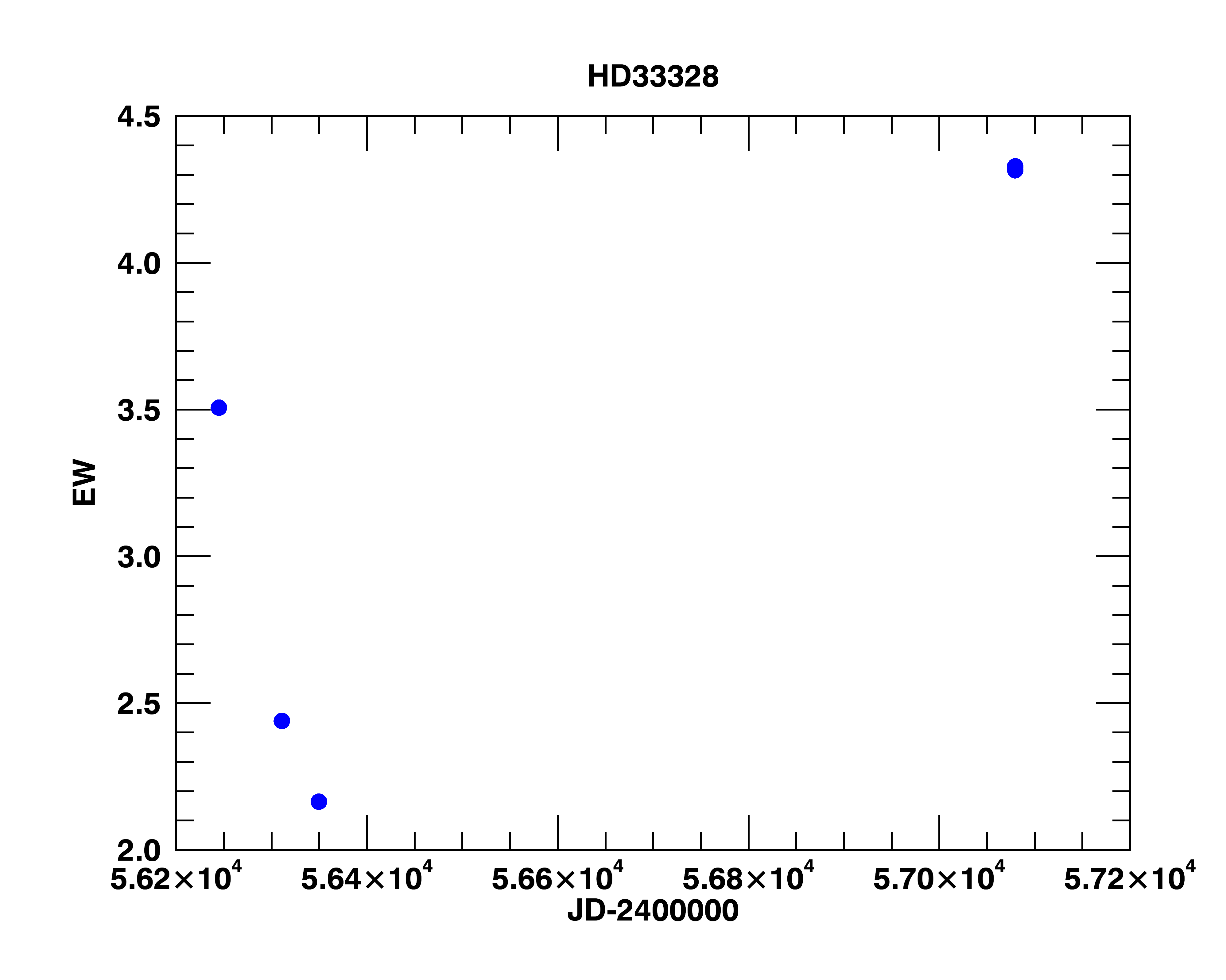
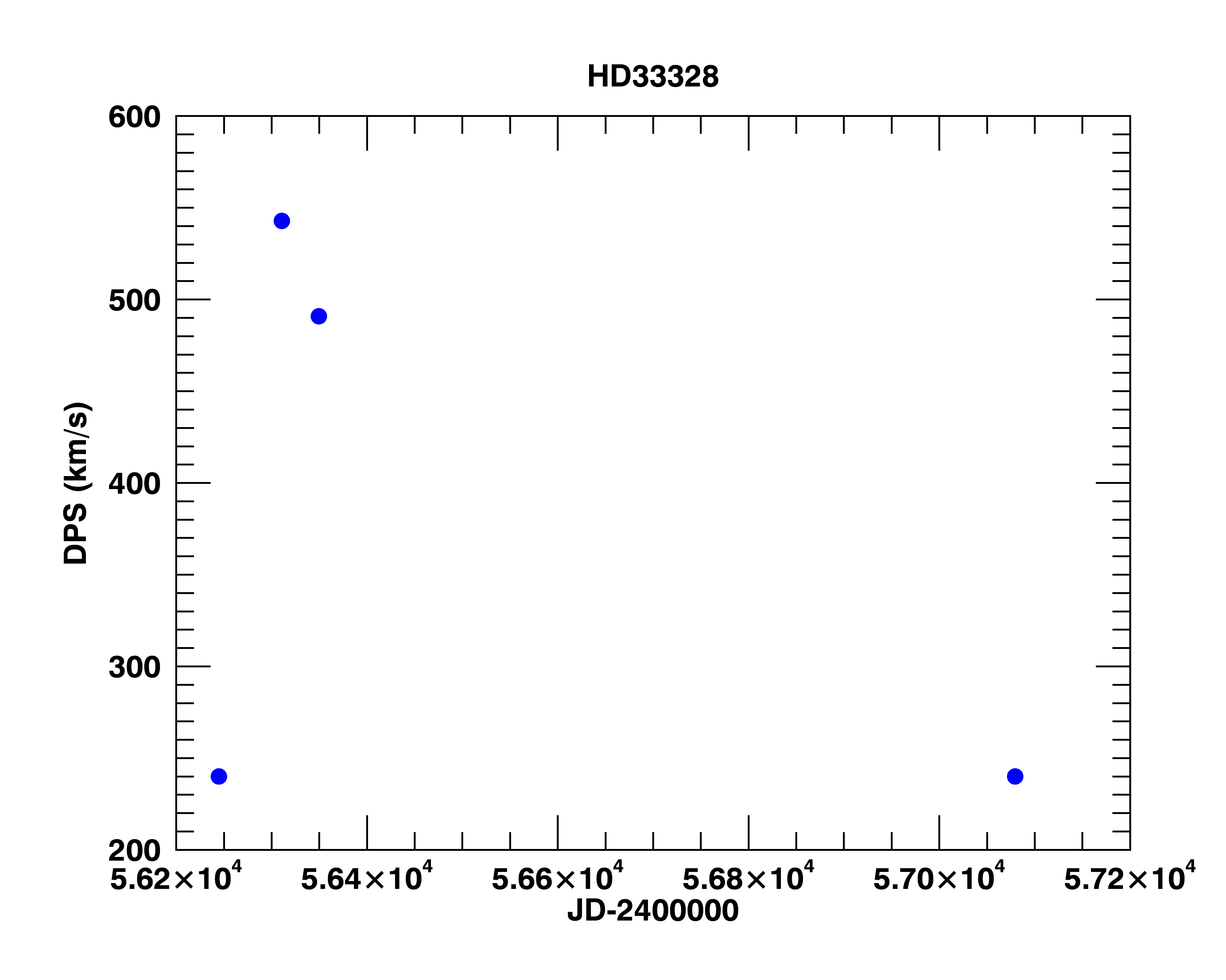
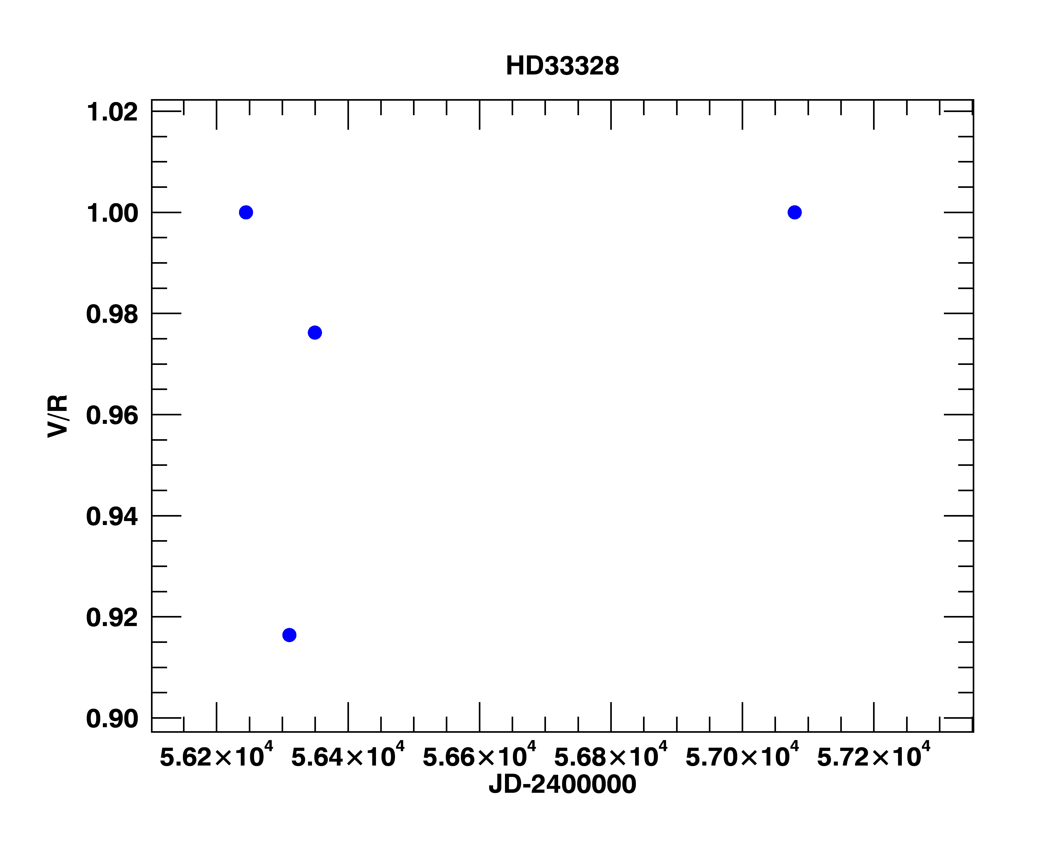
The DPS and V/R are obtained by an interactive IDL program developed for this purpose (MUFIN : MUlti-FitINg). For each spectrum of a target the code searches for the V and R peaks, then the user must decide by visual inspection if the selected point corresponds to the V and R peak, respectively. If not, the user can move freely the interactive bars to fix the point. If the spectrum doesn’t show a double peak line profile, then the user can click on either, “1 peak profile” or “absorption profile”. For the option “1 peak profile” the DPS value is zero and for “absorption profile” the DPS value is set to the width of the H wings of that spectrum. When going through all spectra available for the target, an ASCII file is generated for the DPS and V/R values versus Julian days, as well as their corresponding plots (see Fig. 4).
The accuracy on the measurement of radial velocities depends on a correct wavelength calibration, as well as the correction of the heliocentric velocity. Also it depends on the method used for obtaining the RV values. The methods are:
- •
Cross-correlation method: based on correlating the observed spectrum with a known RVs spectrum, which can be a synthetic, standard or an observed spectrum.
- •
Fitting of line profiles: by fitting the broadened line profile by a Gauss, Voigt or Lorentz distribution. The fitted line center is compared with the observed one.
- •
Mirroring method: comparing the line profile of the observed spectrum with the same line flipped around the laboratory wavelength, and then moving it up to adjust the wings (or core) of the line profile.
There are advantages and disadvantages for each of these different methods. For example, the first two work well on symmetric line profiles, while the mirroring method is efficient for asymmetric profiles but is strongly subjective. Since Be stars usually present asymmetric line profiles, we used the mirroring method to derive RV values. An example of the implementation in MUFIN of this method is shown in Figure 5 for the Be star HD 33328 in the H line profile. The observed and flipped line profiles are represented in red and blue, respectively (left plot). The user can interact with the program to select the continuum section denoted by the green zone in order to derive the error for the calculation. In the right plot of Figure 5, the flipped line profile (blue) is moved to fit the wings of the observed line profile (red). The resulting shift must be divided by 2 taking into account that we only move the flipped line profile. Therefore, the radial velocity value is RV 18.40 km s-1, with a 2.79 and a continuum average of 0.97 0.02. The residual of the fit is shown below each plot. We note that the radial velocity measured changes depending on the region to fix (e.g. the core or the wings), since the origin of this movement is attributed to non-radial pulsations of the central star or the presence of a companion. We obtained values for both regions, core and wings. In the example (see Fig. 6), radial velocities for the Be star HD 33328 from core and wings are change in the opposite way. Further analysis should be made in order to derive the period of this variation and the origin (applying the method used by Aerts et al. (2010)). More data are needed as well as measurements in Helium and metallic lines, since emission and absorption lines of the Balmer series have different values of the radial velocity. Merrill & Sanford (1944) studied the Be shell star 48 Librae and they noted that the radial velocity of the Balmer lines in the shell-phase of the star, became more negative with higher series members. This behavior is known as “Balmer progression”.


Results for all Be stars in the BeSOS website are displayed in the Table 4 (appendix B). Targets are sorted by HD number. Spectral types (Sp.T) and distances (D), taken from the literature, are displayed in the second and third column, respectively. The parameters obtained by the BeSOS’s team are , g, and . The reddening values were also taken from the literature.
Summarizing, relevant information can be obtained analyzing the changes of the H line profile. The global intensity variation as well as the DPS variation are a signature of dissipation/formation of a disk. The V/R variation is a signature of an asymmetry and the RV variation will allow us to detect a possible companion for these objects. More variation aspects will be added in the future such as the superposition of the DPS and intensity in order to find correlations (see Kanaan et al. 2008).
3.3 Late B and early A-type stars
As mentioned before, we constrained the stellar parameters by fitting Tlusty models to the spectroscopic and photometric data where we derive , g, and . For cases with lower temperatures 15000 K, we only give the best SED fit found by fitting Kurucz models. This concerns 16 stars and they are indicated with the superscript letters “LT” in the result Table 4 (Appendix B). For all these targets, values of the DPS, V/R and radial velocity for H emission line are available on the website.
3.4 Getting errors on the measurements
Every parameter given here was found applying an algorithm that minimizes the chi-square value. Once the parameters for each star were fixed, we calculated the confidence intervals using Monte Carlo simulations. The algorithm starts the minimization with a default value for each free parameter, and then once it converges to a minimal Chi-square reduced value, uses a random value to start again the minimization. The random value is chosen from a fixed range previously defined and to converge the algorithm moves between values within 68 (1 standard deviation). The user can set the number of times that the algorithm runs, we set the iteration number to 30. From these 30 iterations, the algorithm chooses the lowest and largest Chi-square reduced values and calculates the standard deviation from the central value, i.e, (Value-Value)/2. As this takes a lot of CPU time, we performed this analysis for one random star of each spectral type. Errors are in general very low, in all cases the percentage deviation does not exceed 1.0 of the original value for and g, and 2.0 for and . The errors are displayed in the results Table (see Table 4). It is important to note that our method does not represent an absolute error for the best fit parameters of each target. In any case the interactive interface (MUFIN) is available for BeSOS users by email request. With this, users can obtain a more realistic error value, either by applying the same method or doing it by “hand”.
4 Results
4.1 Stellar parameters and distribution
Stellar parameters obtained by fitting the spectral energy distribution as well as the HeI and MgII line profiles of each Be star in BeSOS are shown in the Appendix in Table B. Spectral types and distance values from the literature are reported (from the Simbad database), as well as the stellar parameters, , , and derived by the BeSOS team. We noted that spectral types derived here are, in general, hotter than those taken from the literature and with luminosity class V (main sequence stars). As a first result, we explored the projected rotational velocity distribution of our sample and we found a peak between 250 and 300 km s-1 (see left plot of Fig. 7). A secondary peak is seen between 100 and 150 km s-1. Obviously, to search for correlations, we need to deconvolve to compare how the stellar rotation changes with other stellar parameters, e.g., effective temperature. For the moment, we compared our values with the literature (see Frémat et al. (2005) and BeSOS website for sources). The result is shown in the right plot of Figure 7 with a diagonal line as reference. A strong correlation is seen between the values, although in general the values of from the literature are slightly larger than ours.


4.2 New emission line stars
The BeSOS survey is dedicated to the study of the variability of Be stars, but also to discover/confirm new Be stars. To date, we have found one classical Be star and one star showing emission in the H line profile (see Fig. 8).
These stars are poorly studied and there is no information available in the literature about an existing disk, except for HD 42167 where previous work was done deriving the disk parameters in Arcos et al. (2017). The spectral type is taken from the literature and is compared with that obtained in this work.
HD 121492 (HIP67988) is a star with a K0 spectral type and with a visual magnitude of 7.88. We have one spectrum taken in Jan 31, 2014 showing a double peaked H line profile. This object is still not classified, but the SED shows an IR excess in the Far-IR and due to the spectral type the most probable classification is a “Young Stellar Object” (YSO) of Class III. The different dust distributions among the YSO classes result in different SEDs. The classification between classes I to III, depend on the IR-excess slope (from 2 up to 20m), where Class I is for the stronger and Class III is for the weakest IR-excess, respectively (Andre et al., 1993). The SED is shown in the right plot of Figure 9. The best Kurucz model is for = 4736 47 K and g = 2.00 0.02 cm s-2, with = 18.65 0.37 and a distance of 300 12 pc, which corresponds to a K2III spectral type.
HD 42167 ( Col, HR2177, HIP29034) has a B9IV spectral type with a visual magnitude of 4.99. Using our interactive program to fit the photometric data, the best Kurucz model is for = 11430 114 K and g = 3.00 0.03 cm s-2, with = 6.75 0.14 and a distance of 221 9 pc, which corresponds to a B7III spectral type. We have observations from the dates 2014-01-30, 2015-02-25 and 2015-05-06 where the spectra do not show variability during this time. Royer et al. (2002) derived a value of 250 km s-1. The SED is shown in the left plot of the Figure 9.
| Literature/BeSOS | H | H | |||||||
| HD | Sp.T | Date | EW | V/R | DPS | EW | V/R | DPS | |
| (km s-1) | (Å) | (km s-1) | (Å) | (km s-1) | |||||
| 121492 | K0/K2III | – | Jan 31, 2014 | 1.34 | 1.10 | 464.6 | 4.91 | 0.99 | 510.7 |
| 42167 | B9IV/B7III | 250 | Jan 30, 2014 | 2.50 | 0.96 | 229.4 | 4.37 | 1.01 | 305.9 |
| Feb 25, 2015 | 1.97 | 0.95 | 230.6 | 4.26 | 1.02 | 369.6 | |||
| May 06, 2015 | 2.05 | 0.99 | 228.4 | 4.25 | 0.99 | 338.7 | |||

For both objects we calculated V/R, EW and DPS from H and H line profiles, the results are shown in the Table 2.


4.3 Physical models fitted on H emission lines.
Previous work was carried out by Arcos et al. (2017) to study the observed H emission lines of 42 Be stars in the BeSOS survey using radiative transfer codes. In that work, the authors used the non-LTE code BEDISK (Sigut & Jones, 2007) and the auxiliary code BERAY (Sigut, 2011) to solve the transfer equation along a series of rays ( 105) to produce theoretical H line profiles. They took all spectra of each Be star as an independent model to make a statistical study of mass, angular momentum and size of the disk. In total 61 H emission lines were modeled. The parameters of the best fits are displayed in Table 2 of Arcos et al. (2017). Moreover, statistical results were based on a percentage of the representative models (best range of models) for each H emission line, where they found that the disk mass and angular momentum distributions are different between early (B0-B3) and late (B4-B9) subspectral types. Also, they found values of the power-law density distribution (see eq.1 on Arcos et al. (2017)) of -10.4 to -10.2, and 2.0 to 2.5 and disk masses of 3.410-9 and 9.510-10 M⋆ for early and late spectral types, respectively. For the disk size, they calculated the emitting region containing 90 of the total H flux given a range of values concentrated between 10 and 15 stellar radius.
4.4 Complementing other databases
BeSOS is not only a survey of southern Be stars, the main goal is to offer to the user complete information about the targets in the survey. In the literature, a database containing a large number of observed Be stars in the whole sky is the “Be Star Spectra” (BeSS, http://basebe.obspm.fr/basebe/). BeSS is an open database containing spectra from different instruments and telescopes. The majority of southern Be stars with in BeSS have less than 3 spectra in the optical (177 out of 281 Be stars). Moreover 49, 59, and 40 Be stars have respectively 0, 1 and 2 spectra. In the BeSOS survey 23 of these Be stars are already observed. BeSOS, in these cases, completes the data from BeSS, in order, for example, to find variation or observe for the first time the target in the optical range. As an example, we show the star HD 35165 that exhibits a V/R cycle by combining our data with the BeSS data (see Figure 10). We also show three of BeSOS stars containing only one low resolution optical spectrum in BeSS (HD 110335, HD 120324 and HD 127972). In these examples, BeSOS was used to complete BeSS by adding high resolution spectra (see Figure 10). HD 110335 has three different observation epochs, where spectra from BeSOS do not show intensity variation. The flux is almost the same (see EW in the Table 3), but the H double-peak is clearly absent from the BeSS spectrum due to the low resolution (e.g. R=1000). HD 120324 shows a double peaked emission line with intensity and V/R variations. In the case of HD 127972, BeSOS allowed us to find evidence for its shell status with a decrease in its intensity pointing to a dissipating disk phase. Information about these objects: date, observatory site, instrument and resolution are displayed in Table 3, as well as the EW, V/R and DPS, calculated for the H emission line.
| HD | Sp.T | Date | Observatory | Instrument | Resolution | EW | V/R | DPS | |
| (km s-1) | Site | (Å) | (km s-1) | ||||||
| 35165 | B2Vnpe | 350.0 | Oct 19, 2011 | Melbourne | Shelyak eShel | 10000 | -9.4 | 0.98 | 217.0 |
| Dec 01, 2013 | Mirranook | LISA | 1000 | -11.7 | 1.16 | 240.0 | |||
| B4V | 240.0 | Mar 20, 2014 | OUC | PUCHEROS | 17000 | -11.4 | 1.46 | 294.0 | |
| B4V | 240.0 | Nov 14, 2015 | OUC | PUCHEROS | 17000 | -12.5 | 0.56 | 308.0 | |
| Dec 10, 2015 | Shenton Park | LhiresIII | 18000 | -12.6 | 0.54 | 274.0 | |||
| 110335 | B8IV | Jan 30, 2014 | OUC | PUCHEROS | 17000 | -16.2 | 1.0 | 105.0 | |
| B5III | 208.0 | Jun 22, 2014 | Mirranook | LISA | 1000 | -19.8 | – | – | |
| B8IV | May 07, 2015 | OUC | PUCHEROS | 17000 | -16.9 | 1.0 | 112.0 | ||
| 120324 | B2Vnpe | 166 | Apr 23, 2013 | Castanet | ALPY | 600 | -12.3 | – | – |
| B1V | 110.0 | Jan 31, 2014 | OUC | PUCHEROS | 17000 | -12.6 | 1.0 | 97.5 | |
| B1V | 110.0 | Feb 25, 2015 | OUC | PUCHEROS | 17000 | -15.3 | 1.0 | 65.7 | |
| B1V | 110.0 | May 06, 2015 | OUC | PUCHEROS | 17000 | -12.0 | 1.0 | 79.9 | |
| 127972 | B2Ve | 326.0 | Apr 24, 2013 | Castanet | ALPY | 600 | -1.8 | – | – |
| B1V | 240.0 | Jan 31, 2014 | OUC | PUCHEROS | 17000 | -1.8 | 1.0 | 308.4 | |
| B1V | 240.0 | Feb 25, 2015 | OUC | PUCHEROS | 17000 | -0.1 | 1.0 | 319.8 | |
| B1V | 240.0 | May 06, 2015 | OUC | PUCHEROS | 17000 | 0.9 | 0.9 | 376.7 | |
| B1V | 240.0 | Jul 15, 2015 | OUC | PUCHEROS | 17000 | -1.0 | 1.0 | 354.9 |


In the case of HD 35165 observations from various epochs show a clear V/R variation. This kind of variation is associated to a precessing one-armed over density in the disk, and can be modeled using a radiative transfer code (Carciofi et al., 2009). Spectra from BeSS and BeSOS allowed us to estimate the period of this variation. The maximum intensity of the R peak in the available spectra occurred on Dec, 2015 at I 3.3 (V/R = 0.54). If we consider that date as the maximum intensity for the red peak, then by symmetry the violet peak should be at the same maximum intensity, when the red peak is at its minimum. We took the spectrum on Dec, 2015 (BeSS database) and we created a mirrored spectrum. Then, we lowered the spectral resolution of this mirrored spectrum (R=18000) to an instrumental resolution of 1000, and we compared it with the spectrum on Dec, 2013 of the BeSS database. The result is shown in Figure 11, where the dashed blue line corresponds to the mirrored spectrum convoluted with R=1000 and the red line corresponds to the spectrum from BeSS. Based on the similarities of both spectra, we can deduce that the maximum of the violet peak (V/R 1.85) occurred around Dec, 2013.

We do not have enough data to determine a precise period of the V/R cycle variation. By simply fitting a coarse sinusoidal function (assuming V/R 1.85 on Dec, 2013) we estimated a V/R period of 1 year and 4 months ( 480 d). Missing points during the 2012 year and future points could give a better period estimation than the derived period here. The period plot is shown in the Figure 12.

5 Future work
5.1 Interferometry
We have 13 Be stars in BeSOS observed with the instrument AMBER (Petrov et al., 2007), a near-infrared spectro-interferometric instrument of the VLT interferometer. These observations were carried out during October, 2014 in high-resolution mode (HR = 12000) and centered on the Br 2.16 m line to enable the study of the circumstellar gas kinematics through the Doppler effect. To constrain the geometry and kinematics of the disk, we use a model based on the model proposed by Delaa et al. (2011). Further explanation and details can be found in that work. The parameters of this model can be classified as follows:
- •
Global geometric parameters: stellar radius (), distance (), inclination of the system () and disk major-axis position angle in the sky (PA).
- •
Global kinematic parameters: rotational velocity () at the disk inner radius, expansion velocity at the photosphere (), terminal velocity () and exponents of the expansion () and rotation () velocity power laws.
- •
K-band continuum disk geometry: contribution of the continuum () in terms of the Full Width at Half Maximum (FWHM) and the ratio between the flux of the central star and the flux of the envelope ().
- •
Br disk geometry: extension of the Br line-emission region in terms of the FWHM and the EW.
The disk is assumed to be in a Keplerian rotation, therefore the expansion velocity can be negligible and the exponent of the rotation velocity power law takes the value -0.5 (Meilland et al., 2012). Then, the projected rotational velocity is defined as:
| (2) |
where is considered proportional to the critical velocity:
| (3) |
with the polar radius and the distance to the center of the star.
We are working on constraining the stellar and disk parameters of these 13 Be stars by using the optical and infrared spectra, as well as the interferometric observables: differential visibility (V), differential phase () and closure phase (CP). As an example of the model described above, we show the best fit found for the Be star HD 41335. In this case we have one interferometric measurement with AMBER (3 baselines), where the double-peaked line profile, visibility and phase variations present small asymmetries. We set the stellar radius, the distance and the projected rotational velocity to those obtained in the photometric and spectroscopic fit modelling (see Table 4). The EW and the were measured from the Br emission line and the SED, respectively. The values are = 71 and EW(Br) = -12.11 Å. The best fit was found for an inclination angle of i = 70 2 ∘ (giving a rotational velocity 350 5 km s-1) and a PA = 57∘. The fit is relatively good with a value of 3.30. The result is shown in the Figure 13, where the upper panel shows the fit on the emission line (observation in black and model in blue). The lower panel shows the fit of the differential visibility and phase for each baseline (the observation in black and the model in blue). The baselines and position angles are shown above each column plot.


5.2 Supergiant stars
The BeSOS website contains 17 OBA supergiant stars, which were observed to be included as a part of a PhD thesis work on stellar winds (Haucke et al., 2012; Arcos et al., 2014; Haucke et al., 2015, See e.g.,). These stars are observed with the same conditions as the Be stars. The spectra are available for the user, in addition to information from the literature. Measurements on H line profiles will be given over time as these stars show variability in the line because they are losing mass through their strong stellar winds (Castor et al., 1975).
6 Conclusions
BeSOS is a tool that offers to the Be and massive star community a consistent survey of spectra that the user can interactively explore and download. BeSOS contains stellar parameters compiled from the literature, as well as stellar and circumstellar parameters calculated by us based on the spectra, photometric and interferometric data. While BeSOS is an ongoing work, mainly on the analysis part, the user already has access to the data and available analysis at http://besos.ifa.uv.cl.
BeSOS will also allow us to increase the number of Be stars observed and the number of spectra, as well as confirm and discover new Be stars, allowing us to increase the sample for a statistical study. It is important to note that a full study of is being carried out by our team based on the BeSOS survey using the Tlusty code (Hubeny &
Lanz, 1995) and our interferometric observations, in order to derive the inclination angle. This study will be published in BeSOS.
The survey allowed us to discover two new emission lines of which one is a classical Be star (e.g. HD 42167 ).
Finally, we would appreciate if our names (S. Kanaan, C. Arcos L. Vanzi) are considered as co-authors in any work published that makes use of BeSOS data.
Acknowledgements
The authors would like to thank the anonymous referee for suggestions and comments that helped improve this paper, and also to Graeme Candlish for correcting the spelling of this work. S.K. and C.A. acknowledge partial support from FONDECYT Iniciacion throught grant 11130702, CONICYT Capital Humano Avanzado project N 7912010046, Gemini-CONICYT 32120033, PUC observatory for the telescope time used to obtain the spectra and the Centro de Astrofísica de Valparaíso. C.A and I.A acknowledge Fondo Institucional de Becas FIB-UV. C.A thanks to BECAS DE DOCTORADO NACIONAL CONICYT 2016-2017. L.V. acknowledges support from FONDECYT N 1171364. We also acknowledge Patricio Ramirez and Felipe Sobarzo from the Universidad Técnica Federico Santa María, Valparaíso, Chile for developing the BeSOS website. This work has made use of: the BeSS database, operated at LESIA, Observatoire de Meudon, France: http://basebe.obspm.fr, the SIMBAD database, operated at CDS, Strasbourg, France and of the VizieR catalogue access tool, CDS, Strasbourg, France.
References
- Aerts et al. (2010) Aerts C., et al., 2010, A&A, 513, L11
- Andre et al. (1993) Andre P., Ward-Thompson D., Barsony M., 1993, ApJ, 406, 122
- Arcos et al. (2014) Arcos C., Curé M., Kanaan S., Cidale L. S., Haucke M., 2014, in Revista Mexicana de Astronomia y Astrofisica Conference Series. pp 147–147
- Arcos et al. (2017) Arcos C., Jones C. E., Sigut T. A. A., Kanaan S., Curé M., 2017, ApJ, 842, 48
- Brahm et al. (2017) Brahm R., Jordán A., Espinoza N., 2017, PASP, 129, 034002
- Carciofi (2001) Carciofi A. C., 2001, PhD thesis, Instituto de Astronomia, Geofísica e Ciências Atmosféricas, Universidade de São Paulo, Brazil
- Carciofi et al. (2009) Carciofi A. C., Okazaki A. T., Le Bouquin J.-B., Štefl S., Rivinius T., Baade D., Bjorkman J. E., Hummel C. A., 2009, A&A, 504, 915
- Castor et al. (1975) Castor J. I., Abbott D. C., Klein R. I., 1975, ApJ, 195, 157
- Collins (1974) Collins II G. W., 1974, ApJ, 191, 157
- Dachs et al. (1990) Dachs J., Rohe D., Loose A. S., 1990, A&A, 238, 227
- Delaa et al. (2011) Delaa O., et al., 2011, A&A, 529, A87
- Domiciano de Souza et al. (2014) Domiciano de Souza A., et al., 2014, A&A, 569, A10
- Frémat et al. (2005) Frémat Y., Zorec J., Hubert A.-M., Floquet M., 2005, A&A, 440, 305
- Hanuschik (1996) Hanuschik R. W., 1996, A&A, 308, 170
- Haucke et al. (2012) Haucke M., Cidale L. S., Venero R. O. J., Cochetti Y., Torres A., Arcos C., Curé M., 2012, Boletin de la Asociacion Argentina de Astronomia La Plata Argentina, 55, 95
- Haucke et al. (2015) Haucke M., Araya I., Arcos C., Curé M., Cidale L., Kanaan S., Venero R., Kraus M., 2015, in Meynet G., Georgy C., Groh J., Stee P., eds, IAU Symposium Vol. 307, New Windows on Massive Stars. pp 104–105, doi:10.1017/S1743921314006401
- Hubeny & Lanz (1995) Hubeny I., Lanz T., 1995, ApJ, 439, 875
- Infante et al. (2010) Infante L., Guesalaga A., Vanzi L., Jordán A., Padilla N., Guzmán D., 2010, in 25th Texas Symposium on Relativistic Astrophysics. p. 250
- Kanaan et al. (2008) Kanaan S., Meilland A., Stee P., Zorec J., Domiciano de Souza A., Frémat Y., Briot D., 2008, A&A, 486, 785
- Kurucz (1979) Kurucz R. L., 1979, ApJS, 40, 1
- Lee et al. (1991) Lee U., Osaki Y., Saio H., 1991, MNRAS, 250, 432
- Meilland et al. (2007) Meilland A., et al., 2007, A&A, 464, 59
- Meilland et al. (2012) Meilland A., Millour F., Kanaan S., Stee P., Petrov R., Hofmann K.-H., Natta A., Perraut K., 2012, A&A, 538, A110
- Merrill & Sanford (1944) Merrill P. W., Sanford R. F., 1944, ApJ, 100, 14
- Neiner et al. (2011) Neiner C., de Batz B., Cochard F., Floquet M., Mekkas A., Desnoux V., 2011, AJ, 142, 149
- Ochsenbein et al. (2000) Ochsenbein F., Bauer P., Marcout J., 2000, A&AS, 143, 23
- Petrov et al. (2007) Petrov R. G., et al., 2007, A&A, 464, 1
- Porter & Rivinius (2003) Porter J. M., Rivinius T., 2003, PASP, 115, 1153
- Rivinius et al. (2013) Rivinius T., Carciofi A. C., Martayan C., 2013, A&ARv, 21, 69
- Royer et al. (2002) Royer F., Grenier S., Baylac M.-O., Gomez A. E., Zorec J., 2002, VizieR Online Data Catalog, 339, 30897
- Schultz & Wiemer (1975) Schultz G. V., Wiemer W., 1975, A&A, 43, 133
- Sigut (2011) Sigut T. A. A., 2011, in Neiner C., Wade G., Meynet G., Peters G., eds, IAU Symposium Vol. 272, Active OB Stars: Structure, Evolution, Mass Loss, and Critical Limits. pp 426–427, doi:10.1017/S1743921311011045
- Sigut & Jones (2007) Sigut T. A. A., Jones C. E., 2007, ApJ, 668, 481
- Silaj et al. (2016) Silaj J., et al., 2016, ApJ, 826, 81
- Tody (1993) Tody D., 1993, in Hanisch R. J., Brissenden R. J. V., Barnes J., eds, Astronomical Society of the Pacific Conference Series Vol. 52, Astronomical Data Analysis Software and Systems II. San Francisco, Calif. : Astronomical Society of the Pacific, p. 173
- Vanzi et al. (2012) Vanzi L., et al., 2012, MNRAS, 424, 2770
- Vogt et al. (1990) Vogt N., Barrera L. H., Navarro M., 1990, Ap&SS, 173, 145
- Waters et al. (1987) Waters L. B. F. M., Cote J., Lamers H. J. G. L. M., 1987, A&A, 185, 206
- Wenger et al. (2000) Wenger M., et al., 2000, A&AS, 143, 9
- Zorec & Briot (1997) Zorec J., Briot D., 1997, A&A, 318, 443
Appendix A BeSOS’s handbook (online material)
Appendix B Table of the derived stellar parameters
Stellar parameters derived by fitting rotationally convolved stellar model atmospheres (Tlusty) on the lines: HeI 4471 and MgII 4481, and stellar model atmospheres (Kurucz) on photometric data, are presented here. In total we analyzed 69 Be stars, where 16 are considered as Low Temperatures ( 15000K) stars and the results for these stars is based only on the best fit on photometric data (for that reason no value is given). We note that the deviation percentage can be considered as 1.0 for the original value for the and g, and 2.0 for and (see Subsection 3.4).
| Literature | BeSOS | |||||||||
|---|---|---|---|---|---|---|---|---|---|---|
| Target | Sp.T | D | Sp.T | g | E(B-V) | Av | ||||
| (pc) | (K) | (cm s-2) | () | (km s-1) | ||||||
| HD 33328 | B2IVne | 248 11 | B2V | 19526 195 | 3.30 0.03 | 7.31 0.15 | 0.04 | 0.124 | 287 6 | 4.74 |
| HD 35165 | B2Vnpe | 440 106 | B4V | 17000 170 | 4.00 0.04 | 5.90 0.12 | -0.04 | -0.124 | 240 5 | 3.64 |
| HD 35411 | B1V+B2 | 299 95 | B0V | 25900 259 | 4.50 0.04 | 7.70 0.15 | 0.02 | 0.062 | 53 1 | 36.80 |
| HD 35439 | B1Vpe | 318 84 | B1V | 25300 253 | 3.50 0.04 | 4.79 0.10 | 0.04 | 0.124 | 260 5 | 14.28 |
| HD 37041 | O9.5IV | 473 92 | B0V | 27500 275 | 3.72 0.04 | 6.51 0.13 | 0.02 | 0.062 | 140 3 | 40.40 |
| HD 37795LT | B9IVe | 80 2 | B7III | 12200 122 | 3.50 0.04 | 7.00 0.14 | 0.010 | 0.031 | – | 5.10 |
| HD 41335 | B3/5Vne | 403 121 | B1V | 22500 225 | 3.35 0.03 | 7.06 0.14 | 0.14 | 0.434 | 330 7 | 14.17 |
| HD 42167LT | B9IV | 221 8 | B7III | 11430 114 | 3.00 0.03 | 6.75 0.14 | 0.01 | 0.031 | – | 3.40 |
| HD 45725 | B4Veshell | 207 48 | B2V | 19600 196 | 3.40 0.03 | 7.00 0.14 | 0.04 | 0.124 | 280 6 | 1000 |
| HD 45910 | B2IIIe | 752 158 | B1V | 21300 213 | 3.94 0.04 | 9.33 0.19 | 0.409 | 1.268 | 100 2 | 69.17 |
| HD 48917 | B2Ve | 1111 567 | B1V | 22130 221 | 3.30 0.03 | 8.00 0.16 | 0.06 | 0.186 | 200 4 | 14.80 |
| HD 50013 | B1.5Ve | 202 4 | B0V | 26000 260 | 3.90 0.04 | 4.50 0.09 | 0.02 | 0.062 | 290 6 | 22.10 |
| HD 52918 | B1V | 373 30 | B1V | 25450 255 | 4.50 0.04 | 6.50 0.13 | 0.05 | 0.155 | 242 5 | 3.68 |
| HD 56014 | B3IIIe | 531 90 | B2III | 19300 193 | 3.80 0.04 | 10.80 0.22 | 0.00 | 0.00 | 200 4 | 12.5 |
| HD 56139 | B2IV-Ve | 279 13 | B3III | 17170 172 | 3.89 0.04 | 10.50 0.21 | 0.06 | 0.186 | 100 2 | 8.80 |
| HD 57150 | B2V+B3IVne | 246 10 | B1V | 22000 220 | 3.50 0.04 | 6.90 0.14 | 0.14 | 0.434 | 180 4 | 13.40 |
| HD 57219 | B3Vne | 232 12 | B2V | 19300 193 | 3.99 0.04 | 4.69 0.09 | 0.08 | 0.248 | 50 1 | 4.60 |
| HD 57682 | O9.2IV | 1234 0 | B0V | 30000 300 | 4.00 0.04 | 10.30 0.21 | 0.11 | 0.341 | 10 0.2 | 9.30 |
| HD 58343 | B2Vne | 287 47 | B2V | 20000 200 | 3.56 0.04 | 5.39 0.11 | 0.17 | 0.527 | 10 0.2 | 8.37 |
| HD 58715LT | B8Ve | 49 | B7V | 11820 118 | 3.20 0.03 | 3.78 0.08 | 0.02 | 0.062 | – | 5.00 |
| HD 60606 | B2Vne | 363 31 | B3V | 18000 180 | 3.53 0.04 | 6.23 0.12 | 0.02 | 0.062 | 250 5 | 46.00 |
| HD 63462 | B1IVe | 434 43 | B0III | 26000 260 | 2.90 0.03 | 13.50 0.27 | 0.21 | 0.651 | 300 6 | 11.50 |
| HD 68423LT | B6Ve | 250 14 | B7V | 12100 121 | 4.00 0.04 | 4.11 0.08 | 0.02 | 0.062 | – | 3.04 |
| HD 68980 | B2ne | 284 12 | B1V | 23668 237 | 3.32 0.03 | 6.66 0.13 | 0.14 | 0.434 | 110 2 | 10.14 |
| HD 71510 | B2Ve | 213 10 | B3V | 17643 176 | 4.10 0.04 | 4.70 0.09 | 0.08 | 0.248 | 150 3 | 4.80 |
| HD 75311 | B3Vne | 185 4 | B1V | 23895 239 | 4.00 0.04 | 3.00 0.06 | 0.02 | 0.062 | 250 5 | 13.60 |
| HD 78764 | B2IVne | 296 33 | B3III | 19000 190 | 3.80 0.04 | 8.70 0.17 | 0.09 | 0.279 | 140 3 | 5.70 |
| HD 83953 | B5V | 155 4 | B5V | 15000 150 | 2.54 0.03 | 4.00 0.08 | 0.02 | 0.062 | 250 5 | 10.80 |
| HD 89080LT | B8IIIe | 104 | B7III | 11600 116 | 3.50 0.04 | 7.20 0.14 | 0.033 | 0.102 | – | 14.00 |
| HD 89890 | B3IIIe | 352 34 | B5IV | 15000 150 | 3.00 0.03 | 10.07 0.20 | 0.02 | 0.062 | 26.8 0.5 | 21.66 |
| HD 91465 | B4Vne | 148 8 | B3III | 17410 174 | 2.96 0.03 | 7.95 0.16 | 0.09 | 0.279 | 280 6 | 14.60 |
| HD 92938 | B3/5V | 139 3 | B3V | 19000 190 | 3.48 0.03 | 3.30 0.07 | 0.02 | 0.062 | 110 2 | 14.15 |
| HD 93563 | B8/9III | 161 4 | B5III | 15000 150 | 2.30 0.02 | 6.00 0.12 | 0.23 | 0.713 | 280 6 | 15.60 |
| HD 98058LT | A5V | 56 | A4V | 8200 82 | 3.00 0.03 | 3.20 0.06 | 0.02 | 0.124 | – | 12.60 |
| HD 102776 | B3Vne | 182 19 | B2V | 20000 200 | 3.20 0.03 | 5.00 0.10 | 0.02 | 0.062 | 200 4 | 25.70 |
| HD 103192 | ApSi | 94 5 | B8V | 10980 110 | 2.52 0.03 | 3.89 0.08 | 0.00 | 0.00 | – | 3.94 |
| HD 105382 | B3/5IIIe | 134 11 | B5V | 15000 150 | 3.40 0.03 | 4.18 0.08 | 0.02 | 0.062 | 67.5 1.4 | 12.80 |
| HD 105435 | B2Vne | 127 7 | B1V | 22150 222 | 3.43 0.03 | 8.18 0.16 | 0.15 | 0.465 | 250 5 | 15.50 |
| HD 107348LT | B8V | 127 3 | B6V | 12830 128 | 2.26 0.02 | 4.57 0.09 | 0.04 | 0.124 | – | 2.70 |
| HD 110335LT | B5IIIe | 293 21 | B8IV | 10600 106 | 2.90 0.03 | 11.20 0.22 | 0.02 | 0.062 | – | 30.00 |
| HD 110432 | B0.5IVpe | 373 41 | B1V | 22000 220 | 3.00 0.03 | 6.00 0.12 | 0.02 | 0.062 | 400 8 | 70.9 |
| HD 112078 | B3Vne | 117 2 | B4V | 16500 165 | 3.01 0.03 | 3.00 0.06 | 0.03 | 0.093 | 290 6 | 4.46 |
| HD 120324 | B2Vnpe | 155 3 | B1V | 23950 240 | 4.00 0.04 | 5.37 0.11 | 0.02 | 0.062 | 110 2 | 20.20 |
| HD 121492LT | K0 | 505 262 | K2III | 4736 47 | 2.00 0.02 | 18.65 0.37 | 0.40 | 1.244 | – | 20.75 |
| HD 124195 | B5V | 315 35 | B5V | 15000 150 | 4.00 0.04 | 3.80 0.08 | 0.02 | 0.062 | 150 3 | 36.80 |
| HD 124367 | B4Vne | 147 5 | B2V | 19650 197 | 3.00 0.03 | 3.10 0.06 | 0.02 | 0.062 | 260 5 | 51.60 |
| HD 124771 | B4V | 197 8 | B4V | 17100 171 | 3.50 0.04 | 4.30 0.09 | 0.07 | 0.217 | 150 3 | 9.60 |
| HD 127972 | B2Ve | 93 1 | B1V | 21000 210 | 3.95 0.04 | 6.10 0.12 | 0.02 | 0.062 | 240 | 25.40 |
| HD 131492 | B2IV/Ve | 462 62 | B2III | 20000 200 | 4.00 0.04 | 10.80 0.22 | 0.18 | 0.558 | 100 2 | 11.70 |
| HD 135734LT | B8Ve | 102 7 | B6V | 13500 135 | 3.80 0.04 | 3.80 0.08 | 0.03 | 0.093 | – | 26.70 |
| HD 138769 | B3IVp | 131 7 | B3V | 18400 184 | 3.50 0.04 | 3.00 0.06 | 0.02 | 0.062 | 30 0.6 | 58.50 |
| HD 142184 | B2V | 130 7 | B3V | 17375 174 | 4.25 0.04 | 3.03 0.06 | 0.18 | 0.558 | 300 6 | 4.48 |
| HD 142983 | B8Ia/Iab | 143 4 | B3V | 18000 180 | 3.71 0.04 | 3.11 0.06 | 0.08 | 0.257 | 370 7 | 12.90 |
| HD 143275 | B0.3IV | 150 20 | O9V | 30900 309 | 3.50 0.04 | 7.34 0.15 | 0.17 | 0.527 | 257 5 | 13.80 |
| HD 148184 | B2Vne | 161 5 | B0V | 30000 300 | 3.53 0.04 | 4.44 0.09 | 0.40 | 1.240 | 150 3 | 64.00 |
| HD 157042 | B2Vnne | 286 21 | B1V | 22000 220 | 3.90 0.04 | 5.17 0.10 | 0.12 | 0.372 | 280 6 | 11.80 |
| HD 157246 | B1Ib | 341 18 | B1III | 21240 212 | 3.50 0.04 | 14.20 0.28 | 0.08 | 0.248 | 230 5 | 4.70 |
| HD 158427 | B2Vne | 81 5 | B3V | 18110 181 | 3.80 0.04 | 5.07 0.10 | 0.07 | 0.217 | 285 6 | 15.70 |
| HD 167128 | B3II/III | 233 14 | B2V | 20000 200 | 3.80 0.04 | 3.90 0.08 | 0.14 | 0.434 | 50 1 | 10.00 |
| HD 181615LT | F2p | 546 69 | ||||||||
| HD 205637 | B3V | 323 18 | B2V | 20000 200 | 4.10 0.04 | 7.00 0.14 | 0.02 | 0.062 | 230 5 | 24.00 |
| HD 209014LT | B8/9V+B8/9 | 250 30 | B7III | 12200 122 | 3.30 0.03 | 6.00 0.12 | 0.03 | 0.093 | – | 6.10 |
| HD 209409 | B7IVe | 133 4 | B5V | 15000 150 | 3.00 0.03 | 2.90 0.06 | 0.03 | 0.093 | 350 7 | 15.60 |
| HD 212076 | B2IV-Ve | 497 69 | B3III | 18000 180 | 4.00 0.04 | 11.60 0.23 | 0.02 | 0.062 | 100 2 | 20.35 |
- LT
means Low Temperature stars, where the best fit was found only for photometric data.
-
is the reduced Chi-square value obtained for the best fit on photometric data.
-
Information from literature, Sp.T and D, are taken from Simbad database.
| Literature | BeSOS | |||||||||
|---|---|---|---|---|---|---|---|---|---|---|
| Target | Sp.T | D | Sp.T | g | E(B-V) | Av | ||||
| (pc) | (K) | (cm s-2) | () | (km s-1) | ||||||
| HD 212571 | B1III-IVe | 239 16 | B1V | 24500 245 | 3.40 0.03 | 5.90 0.12 | 0.22 | 0.682 | 215 4 | 15.62 |
| HD 214748LT | B8Ve | 149 14 | B7III | 11500 115 | 3.90 0.04 | 6.70 0.13 | 0.01 | 0.031 | – | 3.90 |
| HD 217891 | B6Ve | 125 3 | B4V | 16000 160 | 3.00 0.03 | 3.70 0.07 | 0.04 | 0.124 | 90 2 | 22.60 |
| HD 219688LT | B7/B8V | 123 5 | B5V | 14200 142 | 3.86 0.04 | 3.88 0.08 | 0.00 | 0.00 | – | 3.70 |
| HD 221507LT | B9.5IIIpHgMgSi | 53 | B8V | 11000 110 | 4.40 0.04 | 2.00 0.04 | -0.03 | 0.093 | – | 2.80 |
| HD 224686LT | B8V | 114 2 | B9V | 10500 105 | 3.35 0.03 | 4.30 0.09 | 0.02 | 0.062 | – | 4.58 |
- LT
means Low Temperature stars, where the best fit was found only for photometric data.
-
is the reduced Chi-square value obtained for the best fit on photometric data.
-
Information from literature, Sp.T and D, are taken from Simbad database.