Structural and electronic transformation in low-angle twisted bilayer graphene
Abstract
Experiments on bilayer graphene unveiled a fascinating realization of stacking disorder where triangular domains with well-defined Bernal stacking are delimited by a hexagonal network of strain solitons. Here we show by means of numerical simulations that this is a consequence of a structural transformation of the moiré pattern inherent of twisted bilayer graphene taking place at twist angles below a crossover angle . The transformation is governed by the interplay between the interlayer van der Waals interaction and the in-plane strain field, and is revealed by a change in the functional form of the twist energy density. This transformation unveils an electronic regime characteristic of vanishing twist angles in which the charge density converges, though not uniformly, to that of ideal bilayer graphene with Bernal stacking. On the other hand, the stacking domain boundaries form a distinct charge density pattern that provides the STM signature of the hexagonal solitonic network.
Bilayer graphene (BLG) shares many of the properties of monolayer graphene while also showing a number of pronounced differences. For instance, its equilibrium structural configuration reveals the massive nature of its charge carriers [1], the possibility of inducing a tunable band gap by applying a transverse electric field [2, 3, 4] and quantum Hall valley ferromagnetism [5]. These properties are a result of the coupling between the two layers.
In order to describe the atomic structure of bilayer graphene the relative position of the two layers has to be defined. In many situations it is sufficient to specify a unique interlayer displacement vector that defines the stacking configuration. As a general property of graphitic structures, the low-energy configuration is represented by the Bernal stacking [6, 7]. However, the stacking configuration is not immune to disorder which can manifest, for example, in boundaries that connect two domains with energetically degenerate yet topologically inequivalent stacking configurations, AB and BA [8, 9, 10, 11]. Such stacking domain boundaries are realized by strain solitons, which are segments with a characteristic width where the strain that arises from interfacing two inequivalent stacking domains is confined. Recent studies have shown that strain solitons can be displaced by the action of a scanning tunneling microscope tip, but do not vanish due to their topological nature [12, 8]. From the theoretical point of view, the two-dimensional extension of the Frenkel-Kontorova model predicts the emergence of strain solitons with a typical width of a few nanometers [13] while their density is defined by the twist angle.
In other situations the stacking configuration cannot be uniquely defined on the whole surface of the sample since the two layers cannot be superimposed by a rigid in-plane shift. This is the case of twisted bilayer graphene where one layer is rotated relative to another, a system that has been widely reported in samples grown epitaxially or by chemical vapor deposition [14, 15, 16, 17, 18, 19, 20]. The two rotated layers form a typical moiré superlattice that has been imaged by means of transmission electron microscopy (TEM) and scanning tunneling microscopy (STM). Importantly, strain solitons in bilayer graphene can form a hexagonal network that delimits triangular domains with inequivalent AB and BA Bernal stacking [21, 8, 22]. Remarkably, as pointed out in Ref. [21], such structures are topologically equivalent to twisted BLG.
In this work, we have investigated by means of numerical simulations twisted BLG and show that for twist angles above a crossover angle the equilibrium structures do not differ substantially from a rigid twist of the two layers, while for below a crossover into a different regime takes place. In this regime, the equilibrium configuration consists of a triangular lattice of alternating AB and BA stacking domains separated by shear strain solitons that form a hexagonal network. The electronic structure is profoundly affected by the emergence of this structural phase and exhibits characteristic features determined by the local stacking order. In contrast to the picture valid for low-angle rigidly twisted BLG that predicts low-energy states localized in AA regions [23, 24, 25], we find that the charge density in AB and BA domains resembles that of ideal Bernal-stacked bilayer graphene. On the other hand, the stacking domain boundaries form a distinct charge density pattern that provides the scanning tunneling microscopy signature of the hexagonal solitonic network.
I Results
I.1 Structural transformation in low-angle twisted bilayer graphene
The underlying physical mechanism responsible for the structural transformation occurring in twisted BLG in the limit of small twist angle is the interplay between van der Waals forces, responsible for the interaction between the two graphene layers, and in-plane elasticity forces. As shown in Fig. 1(a), along the diagonal of a moiré supercell of twisted BLG the local stacking evolves through the high-symmetry configurations AA, AB, SP, BA, and AA (see Fig. 1(b) for naming conventions). The binding energy is minimal for AB/BA stacking configuration, whereas AA configuration corresponds to the maximum of the potential energy surface, see Fig. 1(b). The local energy maximum in the middle of the path connecting AB and BA corresponds to an additional high-symmetry stacking configuration commonly referred to as SP. This potential energy landscape leads to in-plane forces that displace atoms in order to maximize the area of AB/BA stacking domains. On the other hand, the in-plane atomic rearrangement is hindered by the strain caused by the atomic displacement itself. The ultimate equilibrium structures result from the competition between the minimization of the interlayer energy and the reaction of the strain field [26].
In our simulations, we investigate the equilibrium structure of twisted bilayer graphene by treating atomic interactions using a classical potential. Previous DFT studies of twisted BLG have been performed within LDA or GGA functionals that disregard dynamical charge correlations responsible for the van der Waals (vdW) interaction [14, 23, 25]. As we aim to treat models with up to atoms, ab initio calculations become prohibitive. Currently available implementations of classical potentials for carbon do not reproduce correctly the interlayer energy of layered structures based on -hybridized carbon atoms [27, 28, 29, 30, 31]. In order to describe correctly the interlayer interaction, we define a new potential formed by a short range contribution, , inherited from the LCBOP potential [28] and a long-range registry-dependent contribution, , described by a reparametrized version of the Kolmogorov-Crespi potential [32]. The parameters of have been fitted in order to reproduce several observables calculated within DFT+vdW (see Section Methods and Supplementary Materials).
Notably, our DFT+vdW calculations reproduce well the equilibrium interlayer distance of graphite and the in-plane bond length . For bilayer graphene, we have found the atomic bond-length and the equilibrium interlayer distances of AB, AA, and SP stacking configurations, respectively, , , and . We have found that the interlayer energies for AA and SP stacking configurations calculated at are, respectively, and relative to AB configuration.

Supercells of twisted bilayer graphene have been built according to the rules derived by imposing commensurability conditions [33, 34]. In particular, one class of supercells is defined by an integer that determines the supercell periodicity vectors and , with and () being the crystal vectors of the graphene honeycomb lattice, and the corresponding twist angle is defined by [33]. Vectors and form a angle and the moiré pattern has symmetry, see Fig. 1(a). Notably, in the limit the twist angle and the supercell linear size are inversely proportional: . We have performed atomic structure relaxation of models with index up to corresponding to , , and total number of atoms .

Figs. 2(a,b) show a model of rigidly twisted BLG with and the corresponding equilibrium structure resulting from relaxation. Upon relaxation, AB(BA) regions have extended and transformed in approximately triangular domains with side, while AA regions reduce to much smaller, nanometer-scale patches in order to minimize the energy penalty payed with respect to Bernal stacking, see Fig. 1(b). The segments separating AB/BA domains form a hexagonal lattice with vertices corresponding to the AA regions. The modulus of the atomic in-plane displacement upon relaxation, , along a high-symmetry path is shown in Fig. 2(d). Along the line connecting point or with point , carbon atoms increasingly displace to restore AB/BA stacking. Because of the opposite value of along segments and , strain concentrates in the vicinity of . When the energy gained by restoring AB or BA stacking order is compensated by the local strain energy, reaches a maximum before abruptly vanishing. The distance between the two symmetric maxima converges to a constant value upon increasing the moiré periodicity . This illustrates the emergence of a shear strain soliton separating two stacking domains. As shown in Fig. 2(f), the modulus of shear strain vector, , corresponds to one carbon-carbon bond length, . A similar reasoning is valid for the path . Additionally, atoms displace in the out-of-plane direction as shown in Fig. 2(c). Out-of-plane relaxation of twisted BLG has been investigated within DFT/LDA for finding out-of-plane corrugation at low twist angles [25]. A work based on a classical potential investigated twisted BLG in the regime [35]. Similarly to what was reported in Ref. [35], we find that approaches the value in AB/BA stacking domains giving rise to the plateaus seen in Fig. 2(c). Moreover, adapts to and , respectively, at and , consistent with the local stacking configurations [36]. Therefore, this leads to a small corrugation (tilt angle of the normal vectors ) at the location of shear solitons as well as their junctions [26, 36].
To obtain a deeper insight into the equilibrium configurations of twisted BLG, we have studied the stacking vector field , defined as the in-plane component of the minimal shift that has to be applied to one layer in order to make it coincide locally with the opposite layer, see Fig. 3(a).

Fig. 3(b) shows the presence of triangular domains with almost constant stacking (white regions). By inspecting the local stacking field around and (side panels in Fig. 3(b)) one can see the confluence of three orientations of differing by . This discontinuity is trivial as the vector for AB(BA) stacking has three degenerate representations forming angles with each other, see Fig. 3(a). However, when following a path connecting one stacking domain with another across a shear soliton, (e.g. from point to point ), rotates by , that is, the stacking configuration changes from AB to BA or vice versa. The variation () is parallel to the strain soliton and coincides with its shear vector. These stacking domain boundaries are topological defects and is assigned as their topological invariant. In the following, the denominations “shear soliton” and “stacking domain boundary” will be used interchangeably.
As shown in Fig. 2(c), along the path has a minimum at , corresponding to SP stacking (). Upon increasing , the full width at half maximum of this dip, , saturates to , a value close to . We choose to use to define the width of the stacking domain boundaries since its determination does not require reference to the corresponding rigidly twisted structure. The calculated widths of the solitons are in good accordance with the experiments [21, 9, 10]. The vertices of the hexagonal network () where six stacking domain boundaries merge are topological point defects with and a non-zero winding number, that is, rotates by along a closed path encompassing [37]. Noteworthy, that in the vicinity of these vertices, due to energetically unfavorable stacking of the latter close to AA, the width of the solitons is smaller than .
Intuitively, we expect that a transformation involving the creation of strain solitons takes place when the twisted BLG supercell is larger than such that the strain field can be efficiently accommodated. The dependence of several observables on (or, equivalently, ) reveals further details of the evolution. As shown in Fig. 4(a), for the distribution of the interlayer distance, , has a minimal spread . Upon reduction of , and increasingly differ and at saturate to = and =, consistent with the data shown in Fig. 2(c). Out-of-plane relaxation competes with the bending rigidity of graphene, estimated as [38]. For lower values of in-plane atomic displacements become non-negligible. Note that the maximum in-plane displacement of individual atoms, , is bounded from above by a half bond length since two inequivalent stacking vectors are connected by and the displacement is equally distributed over the atoms in the two layers. The crossover is underpinned by the change in functional dependence of the density of twist energy on the moiré periodicity: , where is the total energy for a supercell of periodicity , and is the energy of a AB bilayer graphene supercell having the same surface area , see Fig. 4(c). For small values of , atomic in-plane displacements due to relaxation are negligible and the energy required to introduce a twist arises from those regions whose stacking configuration is not AB/BA, which represent a constant fraction of the supercell surface. Thus, the difference is proportional to the surface of the system and the twist energy density equals a constant: . This has been confirmed by DFT calculations, see Fig. S1(c) of Supplementary Informations. On the other hand, for large supercells most of whose area is composed of AB and BA stacking domains, only the soliton network contributes to . As the width of the solitons asymptotically approaches the constant value , the twist energy density is given by , where is the energy per soliton unit length and the factor counts the number of solitons in the moiré supercell. We estimate . The crossover length , corresponding to the crossover angle , is defined as the intersection of the constant line and the curve fitting the two distinct regimes, as shown in Fig. 4(c). Finally, we can rigorously answer why the transformation takes place at large moiré periodicities. Regardless the values of and , the constant “rigid” regime is favorable for , whereas the “solitonic” regime is favorable for .
I.2 Electronic structure of twisted bilayer graphene
The low-energy states of twisted BLG with large to intermediate twist angles can be described by a model that introduces the coupling between graphene layers perturbatively [33, 39, 40]. This model predicts the existence of low-energy massless Dirac fermions with -dependent Fermi velocity and a pair of Van Hove singularities slightly asymmetric with respect to the Dirac point. These predictions have been confirmed experimentally [15, 41, 42, 43]. For smaller twist angles , twisted BLG has been predicted to develop a flat band responsible for a zero-energy peak in the density of states (DOS) [23, 25]. This peak is due to states localized in AA regions as a result of the super-periodic potential induced by the moiré pattern. However, these results cannot be extrapolated to lower values of , as we expect that the structural relaxation suppressing AA-stacked regions strongly affects the electronic structure.
We investigate the low-energy electronic properties of the equilibrium structure of twisted bilayer graphene in the limit by means of a tight-binding model taking into account orbitals with hopping parameters depending on the distance between orbital centers as well as the relative orientation of the orbitals. The latter is achieved by means of the Slater-Koster theory [44], see Supplementary Information for details.
In Fig. 5(a), the band structure for a model with twist angle shows two degenerate Dirac cones projected onto the point of the supercell Brillouin zone, in contrast to the parabolic dispersion of AB graphene [33, 34, 14]. A finite coupling between the states in the two Dirac cones is responsible for low-dispersion bands around the M point, whence the appearance of two low-energy Van Hove singularities in the DOS [33]. We find that the relaxation has negligible effects on the Dirac fermions, except for lifting the degeneracy of the low-energy bands. As the twist angle decreases, the positions of each Van Hove singularity approaches the Dirac energy, eventually merging at . In this regime, the Fermi velocity is zero and the low-energy states are localized in the AA regions. As shown in Fig. 5(b), at the crossover angle the DOS for rigidly twisted BLG shows a triplet of peaks at energies , , and that correspond to the flat low-energy bands observable in the band structure. We have found that the relaxation is responsible for lifting the degeneracy of the central band and shifting the side peaks further away from the Fermi level, however, without introducing qualitative modifications of the electronic structure.

Fig. 6(a) shows the density of states plot for a model characterized by , that is, well below the crossover angle . The DOS of rigidly twisted BLG still exhibits a zero-energy peak with two satellite shoulders. The nature of the low-energy states is revealed by the inspection of local density of states (LDOS) integrated in the energy regions around each of the three peaks, see Fig. 6(b). In all cases the charge density is localized in AA regions and extends on a fraction of surface for the central peak and for satellites, that we found to be largely independent of the moiré periodicity .
The picture changes drastically upon in-plane relaxation responsible for the discussed structural transformation. The DOS of relaxed twisted BLG is overall closer to AB bilayer graphene and, in particular, the zero-energy peak due to the localized states in the AA region is strongly suppressed (Fig. 6(a), inset). We note that the localized states are still present and confined to nanometer-size AA regions, as can be seen in the corresponding LDOS maps (compare Figs. 6(b) and 6(c), central map). The suppression can be explained as follows. In the solitonic regime, for twist angles , relaxation leads to AA regions of constant area. Therefore, upon decreasing twist angle , or equivalently, increasing moiré periodicity , the weight of these states in the total DOS decreases as . This overall decrease of the zero-energy peak weight is expected to be accompanied by its narrowing as suggested previously [45]. However, our numerical calculations performed on large-scale models do not allow to address adequately this effect. The effect of structural relaxation is even more dramatic in the energy ranges corresponding to the side peaks (Fig. 6(c), maps L and R). Indeed, the charge density is partially depleted in AA regions and AB/BA domains show an overall homogeneous distribution, whereas solitons exhibit a slightly larger charge density. Upon closer investigation of the center of an AB domain (point in Fig. 6(d)) one can observe an alternation of atoms with high and low charge density. This is typical of graphene layers with AB stacking configuration as demonstrated by STM images of highly ordered pyrolytic graphite [46]. The reason is the nonequivalence of the two sublattices of AB stacked graphene that reflects different out-of-plane matrix elements for atoms in complementary sublattices. Charge densities in the soliton regions and at the vertices of the network do not show local variations on the atomic scale (Fig. 6(d), points and ). This is consistent with the fact that the stacking configurations SP and AA found in the solitons and in the vertices, respectively, preserve the sublattice equivalence.
II Conclusions
We investigated the equilibrium low-energy structure of twisted bilayer graphene in the limit of vanishing twist angle (down to ) by means of simulations based on a classical potential, which is capable of describing the dependence of the interlayer binding energy on the relative position of the two layers. Carbon atoms displace in order to maximize the area of energetically favorable AB/BA stacking domains that assume a triangular shape. The in-plane strain field, thus, appear confined in a hexagonal network of shear solitons of width , that delimit alternating AB and BA stacking domains. This structural transformation is continuous and takes place at twist angles below the crossover value , at which the moiré superlattice period exceeds the soliton width . In the limit , the equilibrium structure of twisted BLG converges to that of ideal AB-stacked BLG (). However, the convergence is not uniform in the sense that the relative abundance of the AB-stacking regions approaches , but the soliton network due to its topological nature vanishes only at . On the other hand, twisted BLG as such is not stable with respect to AB-stacked BLG () and its existence is governed by kinetic bottlenecks.
This fact has major consequences on the low-energy electronic states of the moiré superlattice. Differently from the range where the DOS of twisted BLG hosts three low-energy peaks due to flat bands of states localized on AA regions, equilibrium structures of twisted BLG with show a DOS resembling that of AB bilayer graphene with a low-energy charge density distribution that can be directly inferred from the local stacking. The charge density is uniform overall in AB/BA-stacked domains, but shows a strong imbalance between the two inequivalent sublattices in each layer. Conversely, the solitons and the network vertices show no breaking of sublattice symmetry. This distinctive pattern enables the identification of the stacking domain boundaries by means of STM experiments. Analogously to the stacking, the relative extent of the regions where the charge distribution differs from that of AB bilayer graphene asymptotically vanishes for .
III Methods
DFT calculations. We have employed the rVV10 functional that treats exchange-correlation energy within the GGA and includes a non-local van der
Waals (vdW) contribution [47, 48] implemented in QUANTUM ESPRESSO [49]. The ion-electron
interaction has been described by means of ultra-soft pseudopotentials [50]. Energy
cutoff for wavefunctions and charge density have been set, respectively,
to and and the
Brillouin zone has been sampled with a Monkhorst-Pack
kpoint grid. All computational parameters and technical details are
listed and discussed in Supplementary Information.
Classical potential simulations. We have employed the long-range
carbon bond order potential (LCBOP) replacing the original long-range
contribution by a reparametrized version of Kolmogorov-Crespi registry-dependent
potential [32] fitted to match
the DFT/rVV10 values of the interlayer binding energy as a function of
interlayer distance and relative shift. The fit has been performed with
the non-linear minimizer provided by DAKOTA code [51].
Additional details about the fit procedure and the resulting parameters can be found in Supplementary
Information. The optimized potential has been implemented in LAMMPS to perform
energy minimizations [52, 53].
Electronic structure calculations. We have considered a Slater-Koster [44] tight-binding model taking into account
orbitals for carbon atoms with hopping parameters depending on the distance between orbital centers
as well as the relative orientation of the orbitals.
This is particularly important in order to describe correctly the interactions
in the soliton region where the relative position of carbon atoms in opposite
layers changes continuously. Since the equilibrium structures show only weak
corrugation, in-plane orbital interactions are predominantly
of the type. For pairs of atoms in opposite layers that are
stacked on top of each other, such as those appearing in AA stacking,
the orbital interaction is purely of character. However, when atoms
are misaligned such as in SP or AB stacking configurations, the interaction is a
mixture of and types. Tight-binding Hamiltonians have been diagonalized using the massively parallel linear algebra library ELPA [54] that allowed us to treat matrices
of order up to . Details on Hamiltonian matrix elements and observable calculations are discussed in Supplementary Information.
IV Acknowledgments
We thank Bastien F. Grosso and Gabriel Autès for collaboration, Riccardo Sabatini, Marco Gibertini and Tommaso Grioni for useful discussions. Anton Kozhevnikov and Luca Marsella assisted us with compiling ELPA libraries. This research was supported by the Swiss NSF grant No. PP00P2_133552 and Graphene Flagship. This work took advantage of the computational facilities of the Swiss National Computing Centre (project s675).
SUPPLEMENTARY INFORMATION
S1 DFT study of interlayer interaction in bilayer graphene
All our DFT calculations are based on the non-local rVV10 functional implemented in QUANTUM ESPRESSO [49]. This functional is composed of the revised-PW86 exchange-correlation functional plus a non-local contribution to account for the van der Waals interaction [55, 50, 47, 48]. Ion-electron interactions have been treated by means of an ultrasoft pseudopotential generated with the revised-PW86 functional [50]. In fact, non-local contributions are not expected to alter the effective potential generated by nuclei and core electrons. As already found for graphite by the authors of the rVV10 functional, relatively high values of wavefunction and charge-density cutoffs, respectively, and , are required to describe accurately -carbon systems. We have used and together with a Monkhorst-Pack k-point grid to obtain converged structural observables. Periodic replicas of the system are separated by of vacuum to guarantee negligible interaction. The interlayer binding energy has been calculated from the total energy, , the energy of one isolated graphene layer, , and the number of atoms in the unit cell, , as follows
| (S1) |
As reported in Ref. [48] and confirmed by our calculations, the atomic bond length of graphite is and the interlayer distance is in accordance with established values [7]. Table S1 reports the interlayer distance and the binding energy for AA and AB bilayer graphene calculated at fixed bond length .
|
Bilayer graphene - AB | Bilayer graphene - AA | |||
|---|---|---|---|---|---|
We have found for AB bilayer graphene the interlayer distance , about larger than for graphite, consistently with previous reports [56]. For AA stacking configuration the equilibrium distance . The dependencies of on and on the interlayer shift, (see Fig. 1(b) of the main text for definition), are shown in Fig. S1(a,b).
S2 Determination of the classical carbon-carbon potential
The classical pair potential for carbon atoms that we have employed in structural relaxations consists in the sum of a short-range contribution and a long-range contribution describing, respectively, covalent bonds and van der Waals interactions between -hybridized carbon atoms. is the short-range term of the LCBOP potential defined in Ref. [28], adopted with no modifications.
The long-range term is a reparametrized version of the registry-dependent potential proposed in Ref. [32]. For a pair of atoms at positions and , with () being the normal vector to the hybridization plane at position (), is defined as
| (S2) | |||
We have made the approximation that normal vectors are directed along the axis. Consequently, . This assumption is justified by the inspection of the corrugation of the equilibrium structures. For all relaxed models we have found that the normal vectors form an angle with the axis. Although the original paper of Kolmogorov and Crespi provides a set of parameters for the potential, we have reparametrized it by fitting Eq. (S2) to three data sets calculated within DFT+vdW. The first two datasets are the binding energy as a function of for AB- and AA-stacked bilayer graphene (see dot data series in Fig. S1) and the third dataset is as a function of at fixed interlayer distance (red symbols in Fig. S1(b)). The fit has been performed employing the non-linear optimizer DAKOTA [51]. Table S2 compares the parameters reported in the original reference and those resulting from our fit.
|
|
|
|
|
|
|
|
| |||||||||||||||||
|---|---|---|---|---|---|---|---|---|---|---|---|---|---|---|---|---|---|---|---|---|---|---|---|---|
|
||||||||||||||||||||||||
| This work |
Fig. S1 shows a remarkable accordance between observables calculated within DFT (symbols data series) and KC potential (continuous curves). In particular, the equilibrium distances calculated by means of the reparametrized KC potential are and , and the respective binding energies for AA and SP stacking configurations calculated at are and relative to AB stacking configuration. Finally, the in-plane carbon-carbon bond length is .
As a test of the transferability of the classical potential resulting from our fit, in Fig. S1(c) we show a comparison of the density of twist energy calculated within DFT and LCBOP/KC for several bilayer graphene models. In particular, we focus on systems with small moiré periodicity (i.e. large twist angles ) in their equilibrium configuration obtained by atomic relaxation. Treating the interlayer interaction classically introduces a discrepancy that is smaller than 10% in most of the cases.
S3 Structural relaxation
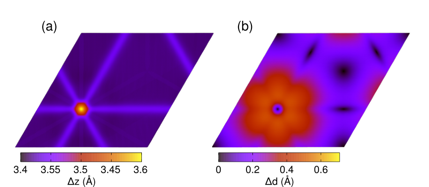
The full potential has been implemented in LAMMPS [52, 53]. Twisted BLG structures have been initially relaxed by means of conjugate gradient plus quadratic line search method [57] and fine minimization was obtained using fast inertia relaxation method [58]. The supercell vectors have been kept fixed and the initial interlayer distance has been set to . At the end of the relaxation the largest force component acting on any atom was below . In Fig. S2, the full maps of the interlayer distance and in-plane atomic displacement are shown. With respect to Fig. 3(c,d) of the main text, the full maps allow to appreciate the whole set of symmetries. is almost constantly equal to along the soliton lines and to in AB/BA domains.
S4 Electronic structure calculations
In this section, we present the details of our electronic structure calculations. The tight-binding model Hamiltonian for bilayer graphene has been taken from Ref. [23] (see also Ref. [24] for thorough electronic structure calculations of rigidly twisted bilayer graphene). In such a model, only -orbitals for carbon atoms are considered. The Hamiltonian is defined as
| (S3) |
where the operators and , respectively, create and annihilate an electron in the -orbital of the atom at position . The matrix elements, , are obtained by combining - and -type Slater-Koster parameters and in the approximation that the axes of -orbitals are parallel, akin to the assumption that the normal vectors of the two graphene layers are parallel. One has
| (S4) |
where is the angle between the orbital axes and the vector connects the two orbital centers [44]. For a pair of atoms in the same layer and . Conversely, for a pair of atoms placed on top of each other in opposite layers, namely forming a dimer, and . and depend exponentially on the distance between the two orbital centers as
| (S5) |
Following Ref. [23] we assume , , , . Differently from Ref. [23], in order to be consistent with the interlayer distance for AB stacking configuration calculated in the present work, we have taken and . The long distance cut-offs for and have been fixed, respectively, at and . We have verified that further increasing these cut-offs does not affect the calculated observables. In all our calculations the charge neutrality point, corresponding to the Fermi energy for undoped systems, is .
Density of states are calculated as follows
| (S6) |
with running over all the eigenvalues at position in reciprocal space. For computational needs the -function appearing in eq. S6 has been replaced by a Lorentzian function:
| (S7) |
The local density of states on the -th atom at position , integrated in the energy range , has been calculated as follows
| (S8) |
where represents the orbital of the -th atom. Spin has not been explicitly considered in our calculations.
Integration over the Brillouin zone have been performed introducing a discrete grid. The band structures shown in panels (a) and (b) of Fig. 5 of the main text have been calculated with a Monkhorst-Pack grid of and k-points, respectively. The density of states of the model shown in Fig. 6 of the main text has been calculated using the high-symmetry points and of the hexagonal Brillouin zone, taking advantage of the fact that the Hamiltonian represented in reciprocal space is a real matrix.
Matrix diagonalizations have been performed employing the Eigenvalue Solvers for Petaflop Applications library (ELPA) [54]. This allowed us to diagonalize a real matrix with in about hours using CPU cores.
References
- [1] A. H. Castro Neto, F. Guinea, N. M. R. Peres, K. S. Novoselov, and A. K. Geim, Rev. Mod. Phys. 81, 109 (2009).
- [2] T. Ohta, A. Bostwick, T. Seyller, K. Horn, and E. Rotenberg, Science 313, 951 (2006).
- [3] J. B. Oostinga, H. B. Heersche, X. Liu, A. F. Morpurgo, and L. M. K. Vandersypen, Nat. Mater. 7, 151 (2008).
- [4] Y. Zhang, T.-T. Tang, C. Girit, Z. Hao, M. C. Martin, A. Zettl, M. F. Crommie, Y. R. Shen, and F. Wang, Nature 459, 820 (2009).
- [5] K. Lee, B. Fallahazad, J. Xue, D. Dillen, K. Kim, T. Taniguchi, K. Watanabe, and E. Tutuc, Science 345, 58 (2014).
- [6] J. D. Bernal, Proceedings of the Royal Society of London A: Mathematical, Physical and Engineering Sciences 106, 749 (1924).
- [7] G. E. Bacon, Acta Crystallog. 4, 558 (1951).
- [8] B. Lalmi, J. C. Girard, E. Pallecchi, M. Silly, C. David, S. Latil, F. Sirotti, and A. Ouerghi, Sci. Rep. 4, 4066 (2014).
- [9] J. Lin, W. Fang, W. Zhou, A. R. Lupini, J. C. Idrobo, J. Kong, S. J. Pennycook, and S. T. Pantelides, Nano Lett. 13, 3262 (2013).
- [10] B. Butz, C. Dolle, F. Niekiel, K. Weber, D. Waldmann, H. B. Weber, B. Meyer, and E. Spiecker, Nature 505, 533 (2014).
- [11] L. Gong, R. J. Young, I. A. Kinloch, S. J. Haigh, J. H. Warner, J. A. Hinks, Z. Xu, L. Li, F. Ding, I. Riaz, R. Jalil, and K. S. Novoselov, ACS Nano 7, 7287 (2013).
- [12] M. Yankowitz, J. I.-J. Wang, A. G. Birdwell, Y.-A. Chen, K. Watanabe, T. Taniguchi, P. Jacquod, P. San-Jose, P. Jarillo-Herrero, and B. J. LeRoy, Nat. Mater. 13, 786 (2014).
- [13] A. M. Popov, I. V. Lebedeva, A. A. Knizhnik, Y. E. Lozovik, and B. V. Potapkin, Phys. Rev. B 84, 045404 (2011).
- [14] J. Hass, F. Varchon, J. E. Millán-Otoya, M. Sprinkle, N. Sharma, W. A. de Heer, C. Berger, P. N. First, L. Magaud, and E. H. Conrad, Phys. Rev. Lett. 100, 125504 (2008).
- [15] G. Li, A. Luican, J. M. B. Lopes dos Santos, A. H. Castro Neto, A. Reina, J. Kong, and E. Y. Andrei, Nat. Phys. 6, 109 (2010).
- [16] L. Brown, R. Hovden, P. Huang, M. Wojcik, D. A. Muller, and J. Park, Nano Lett. 12, 1609 (2012).
- [17] C.-C. Lu, Y.-C. Lin, Z. Liu, C.-H. Yeh, K. Suenaga, and P.-W. Chiu, ACS Nano 7, 2587 (2013).
- [18] K. S. Kim, A. L. Walter, L. Moreschini, T. Seyller, K. Horn, E. Rotenberg, and A. Bostwick, Nat. Mater. 12, 887 (2013).
- [19] T. E. Beechem, T. Ohta, B. Diaconescu, and J. T. Robinson, ACS Nano 8, 1655 (2014).
- [20] I. Razado-Colambo, J. Avila, J.-P. Nys, C. Chen, X. Wallart, M.-C. Asensio, and D. Vignaud, Sci. Rep. 6, 27261 (2016).
- [21] J. S. Alden, A. W. Tsen, P. Y. Huang, R. Hovden, L. Brown, J. Park, D. A. Muller, and P. L. McEuen, Proc. Natl. Acad. Sci. USA 110, 11256 (2013).
- [22] L. Jiang, Z. Shi, B. Zeng, S. Wang, J.-H. Kang, T. Joshi, C. Jin, L. Ju, J. Kim, T. Lyu, Y.-R. Shen, M. Crommie, H.-J. Gao, and F. Wang, Nat. Mater. 15, 840 (2016).
- [23] G. Trambly de Laissardière, D. Mayou, and L. Magaud, Nano Lett. 10, 804 (2010).
- [24] G. Trambly de Laissardière, D. Mayou, and L. Magaud, Phys. Rev. B 86, 125413 (2012).
- [25] K. Uchida, S. Furuya, J.-I. Iwata, and A. Oshiyama, Phys. Rev. B 90, 155451 (2014).
- [26] S. Dai, Y. Xiang, and D. J. Srolovitz, Nano Letters 16, 5923 (2016).
- [27] D. W. Brenner, O. A. Shenderova, J. A. Harrison, S. J. Stuart, B. Ni, and S. B. Sinnott, J. Phys. Condens. Matter 14, 783 (2002).
- [28] J. H. Los and A. Fasolino, Phys. Rev. B 68, 024107 (2003).
- [29] L. Spanu, S. Sorella, and G. Galli, Phys. Rev. Lett. 103, 196401 (2009).
- [30] S. Lebègue, J. Harl, T. Gould, J. G. Ángyán, G. Kresse, and J. F. Dobson, Phys. Rev. Lett. 105, 196401 (2010).
- [31] M. Reguzzoni, A. Fasolino, E. Molinari, and M. C. Righi, Phys. Rev. B 86, 245434 (2012).
- [32] A. N. Kolmogorov and V. H. Crespi, Phys. Rev. B 71, 235415 (2005).
- [33] N. M. R. Lopes dos Santos, J. M. B.and Peres and A. H. Castro Neto, Phys. Rev. Lett. 99, 256802 (2007).
- [34] S. Shallcross, S. Sharma, and O. A. Pankratov, Phys. Rev. Lett. 101, 056803 (2008).
- [35] M. M. v. Wijk, A. Schuring, M. I. Katsnelson, and A. Fasolino, 2D Mater. 2, 034010 (2015).
- [36] S. K. Jain, V. Juričić, and G. T. Barkema, 2D Materials 4, 015018 (2017).
- [37] N. D. Mermin, Rev. Mod. Phys. 51, 591 (1979).
- [38] Y. Wei, B. Wang, J. Wu, R. Yang, and M. L. Dunn, Nano Lett. 13, 26 (2013).
- [39] R. Bistritzer and A. H. MacDonald, Proc. Natl. Acad. Sci. USA 108, 12233 (2011).
- [40] M. Koshino, Phys. Rev. B 88, 115409 (2013).
- [41] A. Luican, G. Li, A. Reina, J. Kong, R. R. Nair, K. S. Novoselov, A. K. Geim, and E. Y. Andrei, Phys. Rev. Lett. 106, 126802 (2011).
- [42] J. Jung, A. M. DaSilva, A. H. MacDonald, and S. Adam, Nat. Commun. 6, 6308 (2015).
- [43] D. Wong, Y. Wang, J. Jung, S. Pezzini, A. M. DaSilva, H.-Z. Tsai, H. S. Jung, R. Khajeh, Y. Kim, J. Lee, S. Kahn, S. Tollabimazraehno, H. Rasool, K. Watanabe, T. Taniguchi, A. Zettl, S. Adam, A. H. MacDonald, and M. F. Crommie, Phys. Rev. B 92, 155409 (2015).
- [44] J. C. Slater and G. F. Koster, Phys. Rev. 94, 1498 (1954).
- [45] P. San-Jose and E. Prada, Phys. Rev. B 88, 121408 (2013).
- [46] W.-T. Pong and C. Durkan, J. Phys. D: Appl. Phys. 38, R329 (2005).
- [47] O. A. Vydrov and T. V. Voorhis, J. Chem. Phys 133, 244103 (2010).
- [48] R. Sabatini, T. Gorni, and S. de Gironcoli, Phys. Rev. B 87, 041108 (2013).
- [49] P. Giannozzi, S. Baroni, N. Bonini, M. Calandra, R. Car, C. Cavazzoni, D. Ceresoli, G. L. Chiarotti, M. Cococcioni, I. Dabo, A. Dal Corso, S. De Gironcoli, S. Fabris, G. Fratesi, R. Gebauer, U. Gerstmann, C. Gougoussis, A. Kokalj, M. Lazzeri, L. Martin-Samos, N. Marzari, F. Mauri, R. Mazzarello, S. Paolini, A. Pasquarello, L. Paulatto, C. Sbraccia, S. Scandolo, G. Sclauzero, A. P. Seitsonen, A. Smogunov, P. Umari, and R. M. Wentzcovitch, J. Phys. Condens. Matter 21, 395502 (2009).
- [50] E. D. Murray, K. Lee, and D. C. Langreth, J. Chem. Theory Comput. 5, 2754 (2009).
- [51] B. Adams, L. Bauman, W. Bohnhoff, K. Dalbey, M. Ebeida, J. Eddy, M. Eldred, P. Hough, K. Hu, J. Jakeman, Swiler, L.P., and D. Vigil, DAKOTA, A Multilevel Parallel Object-Oriented Framework for Design Optimization, Parameter Estimation, Uncertainty Quantification, and Sensitivity Analysis: Version 5.4 User’s Manual (Sandia National Laboratories, 2009).
- [52] S. Plimpton, J. Comput. Phys. 117, 1 (1995).
- [53] “LAMMPS molecular dynamics simulator.” http://lammps.sandia.gov/.
- [54] A. Marek, V. Blum, R. Johanni, V. Havu, B. Lang, T. Auckenthaler, A. Heinecke, H.-J. Bungartz, and H. Lederer, J. Phys. Condens. Matt. 26, 213201 (2014).
- [55] J. P. Perdew and W. Yue, Phys. Rev. B 33, 8800 (1986).
- [56] E. Mostaani, N. Drummond, and V. Fal’ko, Phys. Rev. Lett. 115, 115501 (2015).
- [57] R. Fletcher, Practical Methods of Optimization (John Wiley & Sons, 2013).
- [58] E. Bitzek, P. Koskinen, F. Gähler, M. Moseler, and P. Gumbsch, Phys. Rev. Lett. 97, 170201 (2006).