Randomized Benchmarking Using Unitary $t$-Design for Average Fidelity Estimation of Practical Quantum Circuit

To implement fault-tolerant quantum computation [1] is to design highly reliable quantum circuits. However, there always exists errors for various noise. To remove or decrease the error, we must characterize the errors of quantum circuits first. Use of quantum process tomography (QPT) [2, 3, 4] for error characterization is feasible. In QPT, a known quantum state is used to probe an unknown quantum process to obtain a description of the circuit. These methods can be divided into two types: direct and indirect [5].

In indirect method [6, 7, 8, 9, 10], the QPT is derived from quantum state tomography [11]. Generally, the known input state and the corresponding output results are used to estimate the transfer matrix. However, the indirect QPT approach to noise estimation suffers from several practical deficiencies. Firstly, it is sensitive to state preparation and measurement (SPAM). Secondly, the number of experiments grows exponentially in accordance with increasing the number of qubits and dimensions. Finally, in each experiment, we must calculate an approximated result iteratively; the accuracy of this result is limited by the high computational complexity.

On the other hand, in the direct method, experimental results rather than the transfer matrix directly provide the required information. There has been growing interest in the development of direct QPT for diagnosing noise in quantum circuits, through methods such as direct fidelity estimation [12, 13], gate set tomography [14, 15, 16], and randomized benchmarking [17, 18, 19, 20, 21, 22, 23, 24, 25, 26]. Direct fidelity estimation is a simple method for providing an estimate of the fidelity between a desired quantum process $\Lambda$ and the actual result obtained in the laboratory, up to a constant additive error. However, direct fidelity estimation, which gives an unconditional estimate of the average gate fidelity, is susceptible to SPAM. Gate set tomography provides a full and accurate tomographic description of every gate with confidence bounds. However, although it eliminates the impact of SPAM, considerable resources are required. Randomized benchmarking measures an average error rate that closely estimates the average process infidelity. It is also insensitive to SPAM; thus, it is an efficient method for estimation of the coherence of channel noise [27, 28]. However, it is insensitive to unitary errors [29, 14] and, therefore, cannot measure diamond norm error [30] precisely.

In randomized benchmarking, the average survival probability [31] over all randomized benchmarking sequences $C_{s_{i}}$ of length $r$ is

where $E$ is the measurement operator, $\rho$ is the input state and $C_{s^{-1}}$ is the Clifford gate, which satisfies $C_{s^{-1}}C_{s_{r}}\cdots C_{s_{1}}=|\mathcal{C}|^{r}\mathbb{I}$. The motivation is that the unitary invariance of the Fubini-Study measure make us to turn any Fubini-Study integral into an integral over the Haar measure on $\mathcal{U}(d^{n})$. The average fidelity $\mathbb{E}(F(\psi,U))$ with an input state $|\psi\text{\textrangle}$ and set of unitary operators can be defined as

where the integration of F-S is with respect to the Fubini-Study measure, $\mu_{Haar}(dU)$ denotes the Haar measure, and $|\psi_{0}\text{\textrangle}$ denotes an arbitrary input state. Because the uniform distribution over the Clifford group is an exact unitary $2$-design [32], the average survival probability $P_{r}$ of a sequence of Clifford gates can be efficiently estimated [23].

However, how to construct a multi-qubit Clifford group is currently unknown. For the number of qubit $n=1$, we generally use Clifford gates (i.e. CNOT gates, Hadamard gates and $\pi/4$ phase gates) to construct a Clifford group in randomized benchmarking. For $n\geq 2$, it is not efficient to construct a Clifford group on $n$ qubits for unitary 2-design. Hence, we consider the randomized benchmarking sequences $C_{s_{i}}$ as a polynomial $t$-design (defined in Definition 1). It is equal to the definition of a unitary $t$-design. The advantage of this method is to efficiently construct a random circuit for multi-qubit system.

In this paper, we extend the unitary $t$-design concept,a scheme by which the unitary group is distributed to imitate the characterization of the Haar measure for polynomials of degree up to $t$ [33], for error estimation of a large-scale quantum circuit. It can also be represented in the tensor power $U^{\otimes t}\otimes(U^{\dagger})^{\otimes t}$ of the representation $U$ and its conjugate. There are also many applications of the unitary $t$-design. For example, $t=1$ corresponds to the case of a private quantum channel [34], whereas $t=4$ corresponds to the conditions of the state-distinction problem [35, 36]. Following the extension of the unitary $t$-design, we use local random unitary operator to construct an $\epsilon$-approximate unitary $t$-design, which can be used to analyze the diamond norm error between the arbitrary and uniform distributions of the unitary group. By applying this method, we convert unitary error analysis in practice into an investigation of the pseudo-randomness of the unitary group distribution, which can performed through the analysis of the random walk.

We show below that an exact unitary $t$-design can be constructed using local random unitary operators over a Clifford group on a Markovian noise channel for average fidelity estimation. It is an efficient way to construct the randomized benchmarking sequences for multi-qubit system. We extend the proof of Dankert $et$ $al.$ [32], i.e., that the uniform distribution over the Clifford group is a unitary $2$-design, to a general $t$ by applying a specific decomposition of the local random unitary operators. We then extend the bound of BHH [33] and prove the connection of the spectral gap with a random walk of $n$ steps. We give a bound on the number of sequences required, when performing a unitary $t$-design on $n$-qubit $d$-dimensional system, to obtain an $\epsilon$-approximate unitary $t$-design for arbitrary distribution of a set of unitary operators. Finally, we apply an $\epsilon$-approximate unitary $t$-design to a kind of linear large-scale quantum circuit to estimate the average fidelity and errors caused by practical implementation.

We derive a definition of a polynomial $t$-design as follows, based on Refs. [37, 32].

The above definition gives a method in which the average polynomial over a finite set of unitary operators is rated to an integral with a kind of distribution over $\mathcal{U}(d^{n})$. In randomized benchmarking, a sequence of monomials over a set of unitary operators is generally used to estimate the average infidelity. Meanwhile, a unitary $t$-design is a distribution of a set of unitary operators which mimic properties of the Haar measure for polynomial $t$-design in the tensor power $U^{\otimes t,t}$ of the fundamental representation $U$ and its conjugate. Therefore, a unitary $t$-design can be expressed in terms of quantum operations as follows.

From the above definitions, we derive a strong definition of the $\epsilon$-approximate unitary $t$-design from Ref. [33]. If $\mathcal{N}_{1}$, $\mathcal{N}_{2}$ are superoperators on $n$-qubit $d$-dimensional systems and $|\Phi_{d^{n}}\text{\textrangle}=d^{-n/2}\sum_{i=1}^{d^{n}}|i,i\text{\textrangle}$ is the maximally entangled state, we can define a symbol $\preceq$ as the usual semidefinite ordering such that $\mathcal{N}_{1}\preceq\mathcal{N}_{2}$ satisfies

To simplify the definition, we define an $\epsilon$-approximate unitary $t$-design in terms of the diamond norm i.e.,

where the diamond norm of a superoperator $\Delta$ is defined as in Ref. [38]:

Here, the $p\rightarrow q$ induced Schatten norm is $\textnormal{\textbardbl}\Delta(X)\textnormal{\textbardbl}_{1\rightarrow 1}=\sup_{X\neq 0}\frac{\textnormal{\textbardbl}\Delta(X)\textnormal{\textbardbl}_{p}}{\textnormal{\textbardbl}X\textnormal{\textbardbl}_{q}}$. The diamond norm is generally used as the quantity to prove the fault-tolerance thresholds [39]. Moreover, the diamond norm can be used to indicate the worst-case error rate, where

There is no specific experimental process corresponding to the diamond norm. Therefore, we must scale the bound of the results. However, the complexity of a fidelity estimation increases with the number of qubits $n$. Therefore, it is difficult to find a general solution to directly scale the bound. Here, we follow the approach of Brandao and Horodecki in Ref. [38], using a local random circuit to construct a unitary $t$-design combined with the properties of the random walk to scale the bound.

The properties of local random unitary operators are as follows [38, 40]:

• •

  (Periodic boundary conditions) The (n+1)-th subsystems is identified with the first.

• •

  (Zero ground-state energy) $\lambda_{min}(H_{n,t})=0$, with $\lambda_{min}(H_{n,t})$ being the minimum eigenvalue of $H_{n,t}$.

• •

  (Frustration-freeness) Every state $|\psi\text{\textrangle}$ in the groundstate manifold, composed of all eigenvectors with eigenvalue zero, is such that $H_{i,i+1}|\psi\text{\textrangle}=0$, for all $i\in\{1,\cdots,n\}$.

Our first contribution is to extend the results of Refs. [41, 32].

It is difficult to provide a representation of a large complex multi-qubit system. Therefore, we use the model of local random unitary operators to consider the interaction between two ordering qubits only. Through this approach, the complexity of fidelity estimation is reduced to a great extent. Although this method limits the construction of the practical implementation, it is efficient for obtaining a result to estimate the average fidelity of a quantum process.

Our second contribution is to extend the proof of the results in Ref. [33] rigorously, considering $n$ steps of a random walk.

Because of the normalized local random unitary operator, the diamond norm satisfies

Inserting inequality (12) into inequality 14, we obtain

From FIG. 1, we note that the size of a unitary $t$-design for an arbitrary distribution exhibits exponential growth with increasing $n$. If we take a unitary $t$-design with size larger than $r$ in randomized benchmarking, we can estimate the error caused by pseudo-randomness. In other words, an $\epsilon$-approximate unitary $t$-design with an arbitrary distribution can be used to estimate the unitary error, when its size is larger than $r$. Compared with the factor $n$, the change of $t$ has little effect on $r$.

We can further improve the bound of the diamond norm by relating it to the spectral gap of the local random unitary operator. The aim is to reduce the influence of $n$. Although the error is increased, this approach greatly improves the estimation efficiency.

Our third contribution is to extend the bound of Ref. [33].

From FIG. 2, arbitrary distribution $\nu$ yields an error approaching 1. However, we can use the scheme in Ref. [42] to construct the unitary $t$-design in an experiment. Then, we can estimate the error obtained for a real distribution by applying this method. Hence, we convert the unitary error to an investigation of the pseudo-randomness of a set of unitary operator distributions. The error caused by the experimental pseudo-randomness has a considerable influence on the estimation of the result.

In theory, we establish a boundary for the range of the diamond norm of a given $\epsilon$-approximate unitary $t$-design. In practice, we can recognize the diamond as a quality factor by applying a unitary $t$-design. We can evaluate the randomness by varying the number of unitary selections, which is dependent on only three factors $n$, $r$ and $t$. From FIG. 2, it is apparent that use of small $t$ and large $r$ for estimation of the average fidelity is preferable. However, increased $r$ creates greater complexity with regard to constructing a quantum circuit. Decreased $t$ makes greater needs of unique unitary operators to construct a random circuit in practical randomized benchmarking. Further, from FIG. 1, the change of $t$ has little effect on $r$. Therefore, it is preferable to use the smallest $r$ and largest $t$ to fit the experimental requirements.

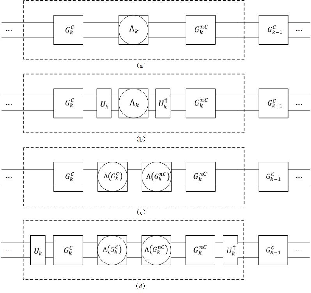
Following the noise circuit in Ref. [25], we construct a quantum circuit that consists of $K$ rounds of subsystems. using a model of a single-qubit unitary 1-design to tailor the gates, Wallman and Emerson separated the circuit into easy and hard gates. However, in the fragment considered here, which is presented in FIG. 3, we use local random unitary operators to construct a unitary $t$-design that can be applied in a kind of large-scale quantum circuit. We separate the circuit into gates constructed using non-trivial Clifford gates and non-Clifford gates. (Note that we add gate $\mathbb{I}$ to the group of non-Clifford gates and use non-Clifford gates as a general designation.) We also denote the noise channel in the circuit as a trace-preserving channel to neglect certain attenuation parameters.

We first consider a Markovian noise channel independent of the gates in the circuit shown in FIG. 3 (a). The circuit consists of only $K$-rounds of subsystems, including a Clifford gate $G_{k}^{C}$, a non-Clifford gate $G_{k}^{nC}$, and a gate-independent channel $\Lambda_{k}$. The fidelity for the input state $|\psi\text{\textrangle}$ and a group of quantum algorithms $\{U_{j}\}$ follows

Our fourth contribution is a fidelity estimation application, performed using an $\epsilon$-approximate unitary $t$-design.

Because it is difficult to find a way to prove that a non-Clifford gate can constitute a unitary $t$-design, we cannot directly estimate the fidelity of the gate-dependent noise channel circuit in FIG. 3 (c). Instead of analyzing the specific noise channel model, however, we can calculate the difference between the gate-dependent and gate-independent noise channel to estimate the approximate range of the results.

Our fifth contribution is the following theorem:

References

• [1] D. Gottesman, Quantum Information Science and Its Contribution to Mathematics 91,13-58 (2009)
• [2] G. M. D’Ariano, M. G. A. Paris, M. F. Sacchi, Advances in Imaging and Electron Physics 128, 205-308 (2003)
• [3] R. Gill, M. Guta, Journal of the Royal Statistical Society 67, 109-134 (2005)
• [4] J. F. Poyatos, J. I. Cirac, P. Zoller, Phys. Rev. Lett. 78, 390-393 (1997)
• [5] M. Mohseni, A. T. Rezakhani, D. A. Lidar, Phys. Rev. A 77, 032322 (2008)
• [6] M. A. Nielsen, I. L. Chuang, Quantum Computation and Quantum Information, 10th ed. (Cambridge Univ. Press, Cambridge [u.a.], 2010)
• [7] D. W. Leung, J. Math. Phys 528-533 (2002)
• [8] G. M. D’Ariano, P. L. Presti, Phys. Rev. Lett. 86, 4195 (2001)
• [9] J. B. Altepeter, D. Branning, E. Jeffrey et al., Phys. Rev. Lett. 90, 193601 (2003)
• [10] G. M. D’Ariano, P. L. Presti, Phys. Rev. Lett. 91, 047902 (2003)
• [11] J. B. Altepeter, D. F. V. James, P. G. Kwiat, in Quantum state estimation, Lecture Notes in Phys. 649, 113-145 (2004)
• [12] M. P. da Silva, O. Landon-Cardinal, D. Poulin, Phys. Rev. Lett. 107, 210404 (2011)
• [13] S. T. Flammia, Y. -K. Liu, Phys. Rev. Lett. 106, 230501 (2011)
• [14] R. Blume-Kohout, J. K. Gamble, E. Nielsen, et al., Nat. Commun. 8 (2017)
• [15] R. Blume-Kohout, J. K. Gamble, E. Nielsen, et al., Nature Physics (2013)
• [16] S. T. Merkel, J. M. Gambetta, J. A. Smolin, et al., Phys. Rev. A 87, 062119 (2013)
• [17] J. Emerson, R. Alicki, K. Zyczkowski, J. Opt. B: Quantum Semiclass. Opt. 7, 347-352 (2005)
• [18] E. Knill, D. Leibfried, R. Reichle, et al., Phys. Rev. A 77, 012307 (2007)
• [19] E. Magesan, J. M. Gambetta, J. Emerson, Phys. Rev. Lett. 106, 180504 (2011)
• [20] E. Magesan, J. M. Gambetta, J. Emerson, Phys. Rev. A 85, 042311 (2012)
• [21] J. P. Gaebler, A. M. Meier, T. R. Tan, et al., Phys. Rev. Lett. 108, 260503 (2012)
• [22] E. Magesan, J. M. Gambetta, B. R. Johnson, et al., Phys. Rev. Lett. 109, 080505 (2012)
• [23] J. J. Wallman, S. T. Flammia, New J. Phys. 16, 103032 (2014)
• [24] J. J. Wallman, M. Barnhill, J. Emerson, New J. Phys. 18, 043021 (2016)
• [25] J. J. Wallman, J. Emerson, Phys. Rev. A 94, 052325 (2016)
• [26] J. Helsen, J. J. Wallman, S. T. Flammia, et al., 1701. 04299v1 (2017)
• [27] J. J. Wallman, C. Granade, R. Harper, et al., New J. Phys. 17,113020 (2015)
• [28] J. J. Wallman, M. Barnhill, J. Emerson, Phys. Rev. Lett. 115, 060501 (2015)
• [29] Y. R. Sanders, J. J. Wallman, B. C. Sanders, New J. Phys. 18, 012002 (2016)
• [30] R. Kueng, D. M. Long, A. C. Doherty, et al., Phys. Rev. Lett. 117, 170502 (2016)
• [31] T. Proctor, K. Rudingfer, K. Young, et al., Phys. Rev. Lett. 118, 130502 (2017)
• [32] C. Dankert, R. Cleve, J. Emerson, et al., Phys. Rev. A 80, 012304 (2009)
• [33] F. G. S. L. Brandao, A. W. Harrow, M. Horodecki, Commun. Math Phys. 346, 397-434 (2016)
• [34] A. Ambainis, M. Mosca, A. Tapp, et al., in 41st Annual Symposium on Foundations of Computer 547-553 (2000)
• [35] P. Sen, arXiv: 0512085v1 (2005)
• [36] A. Ambainis, J. Emerson, arXiv: 0701126v2 (2007)
• [37] J. Emerson, E. Livine, S. Lloyd, Phys. Rev. A 72, 060302 (2005)
• [38] F. G. S. L. Brandao, M. Horodecki, Q. Inf. Comp 13, 0901 (2013)
• [39] D. Aharonov, M. Ben-Or, 29th Acm Symposium on Theory of Computing 38, 176-188 (1997)
• [40] W. G. Brown, L. Viola, Phys. Rev. Lett. 104, 250501 (2009)
• [41] D. P. DiVincenzo, D. W. Leung, B. M. Terhal, IEEE Trans. Inf. Theory 48, 580-599 (2002)
• [42] P. S. Turner, D. Markham, Phys. Rev. Lett. 116, 200501 (2016)
• [43] H. F. Chau, IEEE Trans. Inf. Theory 51, 1451-1468 (2005)
• [44] R. Goodman, N. R¿ Wallach, Symmetry, representations, and invariants Graduate texts in mathematics (2009)
• [45] V. Guruswami, arXiv: 1603.01512 (2016)
• [46] R. Bubley, M. E. Dyer, in 38th Annual Symposium on Foundatins of Computer Science 223 (1997)
• [47] R. I. Oliverira, Annals of Applied Probability 19, 1200-1231 (2009)
• [48] B. Nachtergaele, Commun, Math. Phys. 175, 565-605 (1996)
• [49] B. Schumacher, Physics 54, 3614-2628 (1996)
• [50] C. Ferrie, R. Blume-Kohout, Phys. Rev. Lett. 116, 090407 (2016)
• [51] M. Christandl, R. Renner, Phys. Rev. Lett. 109, 120403 (2012)
• [52] P. Faist, R. Renner, Phys. Rev. Lett. 117, 010404 (2016)
• [53] A. Abeyesinghe, I. Devetak Hayden, et al., Proc. R. Soc. A 465, 2537-2563 (2009)
Appendix A Two steps of random walk acting on three qubit systems
Now we will prove two steps of random walk acting on three qubit systems. Let R1R_{1} and R2R_{2} be two unitaries acting on three qubit dd-dimensional systems. Consider two steps of the walk. Then we have four possibilities, each occurring with probability 1/41/4,
R1→{U~12​U12​R1,U~23​U12​R1,U~12​U23​R1,U~23​U23​R1},R_{1}\rightarrow\{\tilde{U}_{12}U_{12}R_{1},\tilde{U}_{23}U_{12}R_{1},\tilde{U}_{12}U_{23}R_{1},\tilde{U}_{23}U_{23}R_{1}\}, (94)
for independent Haar distributed unitaries U12,U23,U~12,U~23U_{12},U_{23},\tilde{U}_{12},\tilde{U}_{23}, and likewise for R2R_{2}. Here the different indices of the unitaries label in which different subsystems they act non-trivially.
In trivial coupling, the two unitaries R1R_{1} and R2R_{2} must be the same transformation. Then we should consider the nontrivial coupling. We modify the transformation with the unitary V23V_{23} and V12V_{12}, so that U~23​V23\tilde{U}_{23}V_{23} and U~12​V12\tilde{U}_{12}V_{12} are Haar distributed for U~23\tilde{U}_{23} and U~12\tilde{U}_{12}, respectively. We have
R1→R1′={U~12​U12​R1,U~23​V23​U12​R1,U~12​V12​U23​R1,U~23​U23​R1}\begin{split}R_{1}\rightarrow&R_{1}^{\prime}\\ =&\{\tilde{U}_{12}U_{12}R_{1},\tilde{U}_{23}V_{23}U_{12}R_{1},\tilde{U}_{12}V_{12}U_{23}R_{1},\tilde{U}_{23}U_{23}R_{1}\}\end{split} (95)
where the unitary V23V_{23} and V12V_{12} depend on U12U_{12} and U23U_{23}, respectively. And the unitary R2R_{2} undergoes the same transformation as before
R2→R2′={U~12​U12​R2,U~23​U12​R2,U~12​U23​R2,U~23​U23​R2}.R_{2}\rightarrow R_{2}^{\prime}=\{\tilde{U}_{12}U_{12}R_{2},\tilde{U}_{23}U_{12}R_{2},\tilde{U}_{12}U_{23}R_{2},\tilde{U}_{23}U_{23}R_{2}\}. (96)
Then we will show the average of the distance between two unitaries R1R_{1} and R2R_{2} becomes closer after random walk transformation.
𝔼⁡(‖​R1′−R2′​‖2)=14​(𝔼⁡(‖​U~12​U12​R1−U~12​U12​R2​‖22)CLOSE+𝔼⁡(‖​U~23​V23​U12​R1−U~23​U12​R2​‖22)+𝔼⁡(‖​U~12​V12​U23​R1−U~12​U23​R2​‖22)+OPEN𝔼⁡(‖​U~23​U23​R1−U~23​U23​R2​‖22)),\begin{split}&\mathbb{E}(\textnormal{\textbardbl}R_{1}^{\prime}-R_{2}^{\prime}\textnormal{\textbardbl}^{2})\\ =&\frac{1}{4}(\mathbb{E}(\textnormal{\textbardbl}\tilde{U}_{12}U_{12}R_{1}-\tilde{U}_{12}U_{12}R_{2}\textnormal{\textbardbl}_{2}^{2})\\ +&\mathbb{E}(\textnormal{\textbardbl}\tilde{U}_{23}V_{23}U_{12}R_{1}-\tilde{U}_{23}U_{12}R_{2}\textnormal{\textbardbl}_{2}^{2})\\ +&\mathbb{E}(\textnormal{\textbardbl}\tilde{U}_{12}V_{12}U_{23}R_{1}-\tilde{U}_{12}U_{23}R_{2}\textnormal{\textbardbl}_{2}^{2})\\ +&\mathbb{E}(\textnormal{\textbardbl}\tilde{U}_{23}U_{23}R_{1}-\tilde{U}_{23}U_{23}R_{2}\textnormal{\textbardbl}_{2}^{2})),\end{split} (97)
with the expectation taken over Haar distributed U12~,U12,U23~,U23\tilde{U_{12}},U_{12},\tilde{U_{23}},U_{23}. We can rewrite the equation as
𝔼⁡(‖​R1′−R2′​‖)=14​(2​‖​R1−R2​‖22CLOSE+OPEN𝔼⁡(‖​V23​U12​R1−U12​R2​‖22)+𝔼⁡(‖​V12​U23​R1−U23​R2​‖22)).\begin{split}&\mathbb{E}(\textnormal{\textbardbl}R_{1}^{\prime}-R_{2}^{\prime}\textnormal{\textbardbl})=\frac{1}{4}(2\textnormal{\textbardbl}R_{1}-R_{2}\textnormal{\textbardbl}_{2}^{2}\\ +&\mathbb{E}(\textnormal{\textbardbl}V_{23}U_{12}R_{1}-U_{12}R_{2}\textnormal{\textbardbl}_{2}^{2})+\mathbb{E}(\textnormal{\textbardbl}V_{12}U_{23}R_{1}-U_{23}R_{2}\textnormal{\textbardbl}_{2}^{2})).\end{split} (98)
Since V12V_{12} and V23V_{23} can depend in arbitrary way on U23U_{23} and U12U_{12}, respectively, we can take the minimum over V12V_{12} and V23V_{23} to get
𝔼⁡(‖​R1′−R2′​‖2)=14​(2​‖​R1−R2​‖22CLOSE+𝔼⁡(minV23⁡‖​V23​U12​R1−U12​R2​‖22)+OPEN𝔼⁡(minV12⁡‖​V12​U23​R1−U23​R2​‖)).\begin{split}&\mathbb{E}(\textnormal{\textbardbl}R_{1}^{\prime}-R_{2}^{\prime}\textnormal{\textbardbl}^{2})\\ =&\frac{1}{4}(2\textnormal{\textbardbl}R_{1}-R_{2}\textnormal{\textbardbl}_{2}^{2}\\ +&\mathbb{E}(\min_{V_{23}}\textnormal{\textbardbl}V_{23}U_{12}R_{1}-U_{12}R_{2}\textnormal{\textbardbl}_{2}^{2})\\ +&\mathbb{E}(\min_{V_{12}}\textnormal{\textbardbl}V_{12}U_{23}R_{1}-U_{23}R_{2}\textnormal{\textbardbl})).\end{split} (99)
Then, for any two unitaries R1R_{1} and R2R_{2} we have
‖​R1−R2​‖22=2​(t​r​(𝕀)−R​e​(t​r​(R1​R2†))).\textnormal{\textbardbl}R_{1}-R_{2}\textnormal{\textbardbl}_{2}^{2}=2(tr(\mathbb{I})-Re(tr(R_{1}R_{2}^{\dagger}))). (100)
Since R1R_{1} and R2R_{2} are infinitesimally close we can write
R=R1​R2†=ei​ϵ​H=𝕀+i​ϵ​H−ϵ22​H2+O⁡(ϵ3)R=R_{1}R_{2}^{\dagger}=e^{i\epsilon H}=\mathbb{I}+i\epsilon H-\frac{\epsilon^{2}}{2}H^{2}+O(\epsilon^{3}) (101)
for a Hermitian matrix HH with ‖​H​‖2≤1\textnormal{\textbardbl}H\textnormal{\textbardbl}_{2}\leq 1. Then we get
‖​R1−R2​‖22=2​(t​r​(𝕀)−R​e​(t​r​(R1​R2†)))=2​(t​r​(𝕀)−R​e​(t​r​(𝕀+i​ϵ​H−ϵ22​H2−i​ϵ36​H3+O⁡(ϵ4))))=ϵ2​t​r​(H2)+O⁡(ϵ4)\begin{split}&\textnormal{\textbardbl}R_{1}-R_{2}\textnormal{\textbardbl}_{2}^{2}=2(tr(\mathbb{I})-Re(tr(R_{1}R_{2}^{\dagger})))\\ =&2(tr(\mathbb{I})-Re(tr(\mathbb{I}+i\epsilon H-\frac{\epsilon^{2}}{2}H^{2}-i\frac{\epsilon^{3}}{6}H^{3}+O(\epsilon^{4}))))\\ =&\epsilon^{2}tr(H^{2})+O(\epsilon^{4})\end{split} (102)
Consider the term 𝔼⁡(minV12⁡‖​V12​U23​R1−U23​R2​‖22)\mathbb{E}(\min_{V_{12}}\textnormal{\textbardbl}V_{12}U_{23}R_{1}-U_{23}R_{2}\textnormal{\textbardbl}_{2}^{2}) in the right side of the above equation. (The other terms have the similar results.) We have
𝔼⁡(minV12⁡‖​V12​U23​R1−U23​R2​‖22)=2​(t​r​(𝕀)−𝔼⁡(maxV12⁡|R​e​(t​r​(V12​U23​R1​R2†​U23†))|))=2​(t​r​(𝕀)−𝔼​‖​t​r3​(U23​R​U23†)​‖1),\begin{split}&\mathbb{E}(\min_{V_{12}}\textnormal{\textbardbl}V_{12}U_{23}R_{1}-U_{23}R_{2}\textnormal{\textbardbl}_{2}^{2})\\ =&2(tr(\mathbb{I})-\mathbb{E}(\max_{V_{12}}|Re(tr(V_{12}U_{23}R_{1}R_{2}^{\dagger}U_{23}^{\dagger}))|))\\ =&2(tr(\mathbb{I})-\mathbb{E}\textnormal{\textbardbl}tr_{3}(U_{23}RU_{23}^{\dagger})\textnormal{\textbardbl}_{1}),\end{split} (103)
where, ‖​X​‖1=maxU∈𝕌⁡|t​r​(U​X)|\textnormal{\textbardbl}X\textnormal{\textbardbl}_{1}=\max_{U\in\mathbb{U}}|tr(UX)|. Then, we get
‖​t​r3​(U23​R​U23†)​‖1=‖​t​r3​(𝕀+i​ϵ​U23​H​U23†−ϵ22​U23​H2​U23†+O⁡(ϵ3))​‖1=‖​t​r3​(𝕀+i​ϵ​U23​H​U23†)−ϵ22​t​r3​(U23​H2​U23†)+O⁡(ϵ3)​‖1=‖​t​r3​(ei​ϵ​U23​H​U23†+ϵ22​(U23​H​U23†)2)−ϵ22​t​r3​(U23​H2​U23†)+O⁡(ϵ3)​‖1=t​r​(𝕀)+ϵ22​1d​t​r​((t​r3​(U23​H​U23†))2)−ϵ22​t​r​(H2)+O⁡(ϵ3),\begin{split}&\textnormal{\textbardbl}tr_{3}(U_{23}RU_{23}^{\dagger})\textnormal{\textbardbl}_{1}\\ =&\textnormal{\textbardbl}tr_{3}(\mathbb{I}+i\epsilon U_{23}HU_{23}^{\dagger}-\frac{\epsilon^{2}}{2}U_{23}H^{2}U_{23}^{\dagger}+O(\epsilon^{3}))\textnormal{\textbardbl}_{1}\\ =&\textnormal{\textbardbl}tr_{3}(\mathbb{I}+i\epsilon U_{23}HU_{23}^{\dagger})-\frac{\epsilon^{2}}{2}tr_{3}(U_{23}H^{2}U_{23}^{\dagger})+O(\epsilon^{3})\textnormal{\textbardbl}_{1}\\ =&\textnormal{\textbardbl}tr_{3}(e^{i\epsilon U_{23}HU_{23}^{\dagger}}+\frac{\epsilon^{2}}{2}(U_{23}HU_{23}^{\dagger})^{2})-\frac{\epsilon^{2}}{2}tr_{3}(U_{23}H^{2}U_{23}^{\dagger})+O(\epsilon^{3})\textnormal{\textbardbl}_{1}\\ =&tr(\mathbb{I})+\frac{\epsilon^{2}}{2}\frac{1}{d}tr((tr_{3}(U_{23}HU_{23}^{\dagger}))^{2})-\frac{\epsilon^{2}}{2}tr(H^{2})+O(\epsilon^{3}),\end{split} (104)
so that we get
𝔼​infV12‖​V12​U23​R1−U23​R2​‖22=ϵ2​[t​r​(H2)−1d​𝔼​(t​r​((t​r3​(U23​H​U23†))2))]+O⁡(ϵ3).\begin{split}&\mathbb{E}\inf_{V_{12}}\textnormal{\textbardbl}V_{12}U_{23}R_{1}-U_{23}R_{2}\textnormal{\textbardbl}_{2}^{2}\\ =&\epsilon^{2}[tr(H^{2})-\frac{1}{d}\mathbb{E}(tr((tr_{3}(U_{23}HU_{23}^{\dagger}))^{2}))]+O(\epsilon^{3}).\end{split} (105)
Now our goal is to compute the average 𝔼⁡(t​r​((t​r3​(U23​H​U23†))2))\mathbb{E}(tr((tr_{3}(U_{23}HU_{23}^{\dagger}))^{2})). We note that for any operator C123C_{123} we have [53]
tr(C122)=tr((C123⊗C123¯)(𝔽12:12¯⊗𝕀3:3¯))tr(C_{12}^{2})=tr((C_{123}\otimes C_{\overline{123}})(\mathbb{F}_{12:\overline{12}}\otimes\mathbb{I}_{3:\overline{3}})) (106)
where systems with bars are copies of original systems, and 𝔽\mathbb{F} is the operator which swaps systems 12 with 12¯\overline{12}. Therefore
𝔼⁡(t​r​((t​r3​(U23​H​U23†))2))=𝔼(tr((H123⊗H123¯)(U23†⊗U23¯†)(𝔽12:12¯⊗𝕀3:3¯)(U23⊗U23¯))).\begin{split}&\mathbb{E}(tr((tr_{3}(U_{23}HU_{23}^{\dagger}))^{2}))\\ =&\mathbb{E}(tr((H_{123}\otimes H_{\overline{123}})(U_{23}^{\dagger}\otimes U_{\overline{23}}^{\dagger})(\mathbb{F}_{12:\overline{12}}\otimes\mathbb{I}_{3:\overline{3}})(U_{23}\otimes U_{\overline{23}}))).\end{split} (107)
We now compute
𝔼((U23†⊗U23¯†)(𝔽2:2¯⊗𝕀3:3¯)(U23⊗U23¯))=dd2+1(𝕀23:23¯+𝔽23:23¯).\mathbb{E}((U_{23}^{\dagger}\otimes U_{\overline{23}}^{\dagger})(\mathbb{F}_{2:\overline{2}}\otimes\mathbb{I}_{3:\overline{3}})(U_{23}\otimes U_{\overline{23}}))=\frac{d}{d^{2}+1}(\mathbb{I}_{23:\overline{23}}+\mathbb{F}_{23:\overline{23}}). (108)
Using the fact that the tensor product of swap operators is again a swap operator(e.g. 𝔽12:12¯=𝔽1:1¯⊗𝔽2:2¯\mathbb{F}_{12:\overline{12}}=\mathbb{F}_{1:\overline{1}}\otimes\mathbb{F}_{2:\overline{2}}), we obtain
𝔼⁡(t​r​((t​r3​(U23​H​U23†))2))=dd2+1(tr((H123⊗H123¯)𝔽123:123¯+(H123⊗H123¯)𝔽1:1¯⊗𝕀23:23¯))=dd2+1​(t​r​(H2)+t​r​(H12))≥dd2+1​t​r​(H2).\begin{split}&\mathbb{E}(tr((tr_{3}(U_{23}HU_{23}^{\dagger}))^{2}))\\ =&\frac{d}{d^{2}+1}(tr((H_{123}\otimes H_{\overline{123}})\mathbb{F}_{123:\overline{123}}\\ +&(H_{123}\otimes H_{\overline{123}})\mathbb{F}_{1:\overline{1}}\otimes\mathbb{I}_{23:\overline{23}}))\\ =&\frac{d}{d^{2}+1}(tr(H^{2})+tr(H_{1}^{2}))\\ \geq&\frac{d}{d^{2}+1}tr(H^{2}).\end{split} (109)
Hence we obtain
infV12𝔼⁡(‖​V12​U23​R1−U23​R2​‖22)≤ϵ2​(1−1d2+1)​t​r​(H2)+O⁡(ϵ3).\inf_{V_{12}}\mathbb{E}(\textnormal{\textbardbl}V_{12}U_{23}R_{1}-U_{23}R_{2}\textnormal{\textbardbl}_{2}^{2})\leq\epsilon^{2}(1-\frac{1}{d^{2}+1})tr(H^{2})+O(\epsilon^{3}). (110)
Finally, we get
𝔼⁡(‖​R1′−R2′​‖2)≤ϵ2​(1−12​1d2+1)​t​r​(H2)+O⁡(ϵ3).\mathbb{E}(\textnormal{\textbardbl}R_{1}^{\prime}-R_{2}^{\prime}\textnormal{\textbardbl}^{2})\leq\epsilon^{2}(1-\frac{1}{2}\frac{1}{d^{2}+1})tr(H^{2})+O(\epsilon^{3}). (111)
The fact that ∫𝒰⁡(dn)U⊗t,t​ν​(𝑑U)\int_{\mathcal{U}(d^{n})}U^{\otimes t,t}\nu(dU) is a projector that
g⁡(ν∗k,t)=g​(ν,t)k.g(\nu^{\ast k},t)=g(\nu,t)^{k}. (112)
Then, applying Lemma 1
lim supε→0supU1,U2∈𝕌⁡(d3){W2​((ν3,d)∗2​νU1,(ν3,d)∗2​νU2)‖​U1−U2​‖2:‖U1−U2‖2≤ε}≤C:=(1−241d2+1)12.\begin{split}\limsup_{\varepsilon\rightarrow 0}\sup_{U_{1},U_{2}\in\mathbb{U}(d^{3})}\{&\frac{W_{2}((\nu_{3,d})^{\ast 2}\nu_{U_{1}},(\nu_{3,d})^{\ast 2}\nu_{U_{2}})}{\textnormal{\textbardbl}U_{1}-U_{2}\textnormal{\textbardbl}_{2}}:\\ &\textnormal{\textbardbl}U_{1}-U_{2}\textnormal{\textbardbl}_{2}\leq\varepsilon\}\leq C:=(1-\frac{2}{4}\frac{1}{d^{2}+1})^{\frac{1}{2}}.\end{split} (113)
Since maxU1,U2⁡‖​U1−U2​‖2≤2​d3/2\max_{U_{1},U_{2}}\textnormal{\textbardbl}U_{1}-U_{2}\textnormal{\textbardbl}_{2}\leq\sqrt{2}d^{3/2} with U1,U2∈𝒰⁡(d3)U_{1},U_{2}\in\mathcal{U}(d^{3}), we get
W⁡(ν,μH​a​a​r)≤W2​((ν3,d)∗2​νU1,(ν3,d)∗2​νU2)≤(1−12​1d2+1)12​2​d32.\begin{split}W(\nu,\mu_{Haar})\leq&W_{2}((\nu_{3,d})^{\ast 2}\nu_{U_{1}},(\nu_{3,d})^{\ast 2}\nu_{U_{2}})\\ \leq&(1-\frac{1}{2}\frac{1}{d^{2}+1})^{\frac{1}{2}}\sqrt{2}d^{\frac{3}{2}}.\end{split} (114)
Appendix B Haar measure of Monomials
We followed the generalization of Haar average of state-component monomials in Ref. [36].
∑π∈𝒮t|⟨​ψσ,d​|ψπ,d​⟩|n=1dt​n​∑π∈𝒮tt​r​(Vdn​(π)​Vdn​(σ)T)=1dt​n​∑π∈𝒮tt​r​(Vdn​(π​σ−1))=1dt​n​∑π∈𝒮tt​r​(Vdn​(π))=t!dt​n​t​r​(Ps​y​m,t,dn),\begin{split}\sum_{\pi\in\mathcal{S}_{t}}|\text{\textlangle}\psi_{\sigma,d}|\psi_{\pi,d}\text{\textrangle}|^{n}&=\frac{1}{d^{tn}}\sum_{\pi\in\mathcal{S}_{t}}tr(V_{d^{n}}(\pi)V_{d^{n}}(\sigma)^{T})\\ &=\frac{1}{d^{tn}}\sum_{\pi\in\mathcal{S}_{t}}tr(V_{d^{n}}(\pi\sigma^{-1}))\\ &=\frac{1}{d^{tn}}\sum_{\pi\in\mathcal{S}_{t}}tr(V_{d^{n}}(\pi))\\ &=\frac{t!}{d^{tn}}tr(P_{sym,t,d^{n}}),\end{split} (115)
with Ps​y​m,t,dnP_{sym,t,d^{n}} the projector onto the symmetric subspace of (ℂdn)⊗t(\mathbb{C}^{d^{n}})^{\otimes t}:
Ps​y​m,t,dn=1t!​∑π∈𝒮tVdn​(π).P_{sym,t,d^{n}}=\frac{1}{t!}\sum_{\pi\in\mathcal{S}_{t}}V_{d^{n}}(\pi). (116)
Consider a set of unitary operators in dnd^{n}-dimensional Hilbert space, ℋ=ℂdn\mathcal{H}=\mathbb{C}^{d^{n}} consisting of the set of normalized pure states. These states correspond to the points of a unit sphere 𝕊2​dn−1\mathbb{S}^{2d^{n}-1} which is the ”surface” of a ball in 2​dn2d^{n} real dimensions. There exists a unique natural measure that is induced by the invariant (Haar) measure on the unitary group 𝒰⁡(dn)\mathcal{U}(d^{n}): a uniformly random pure state can be defined by the action of a uniformly random unitary matrix on an arbitrary reference state. The measure on pure states is distinguished by the rotational invariance of the Haar measure, which we will denote as μH​a​a​r(U|ψ⟩)\mu_{Haar}(U_{|\psi\text{\textrangle}}). Choosing a fixed representation, U|ψ⟩=|ψ⟩⟨ψ|=∑ici2U|i⟩U_{|\psi\text{\textrangle}}=|\psi\text{\textrangle\textlangle}\psi|=\sum_{i}c_{i}^{2}U_{|i\text{\textrangle}} where |ψ⟩=∑ici|i⟩|\psi\text{\textrangle}=\sum_{i}c_{i}|i\text{\textrangle}. The uniform measure for normalized vectors in ℋ\mathcal{H} can be expressed using the Euclidean parametrization,
μH​a​a​r(dU|ψ⟩:ψ∈𝕊dn)=(∏i=1dnd2ci)δ(∑l=1dn|cl|2−1)\mu_{Haar}(dU_{|\psi\text{\textrangle}}:\psi\in\mathbb{S}^{d^{n}})=(\prod_{i=1}^{d^{n}}d^{2}c_{i})\delta(\sum_{l=1}^{d^{n}}|c_{l}|^{2}-1) (117)
where δ\delta is the Dirac delta function.
The average value of any function f:ℋ→ℂf:\mathcal{H}\rightarrow\mathbb{C} takes the explicit form,
⟨f(U)⟩ψ=1V𝕊2​dn−1f(U)μH​a​a​r(dU⟨​ψ​⟩:ψ∈𝕊2​dn−1).\text{\textlangle}f(U)\text{\textrangle}_{\psi}=\frac{1}{V_{\mathbb{S}^{2d^{n}-1}}}f(U)\mu_{Haar}(dU_{\text{\textlangle}\psi\text{\textrangle}}:\psi\in\mathbb{S}^{2d^{n}-1}). (118)
Consider first calculating the volume of the unitary operators. We have
V𝕊2​dn−1=∫𝕊2​dn−1μH​a​a​r​(𝑑U)\displaystyle V_{\mathbb{S}^{2d^{n}-1}}=\int_{\mathbb{S}^{2d^{n}-1}}\mu_{Haar}(dU) (119)
=\displaystyle= ∫𝕊2​dn−1(∏i=1dnd2​uir)​(∑l=1dn|ul|2r2−1)\displaystyle\int_{\mathbb{S}^{2d^{n}-1}}(\prod_{i=1}^{d^{n}}d^{2}\frac{u_{i}}{r})(\frac{\sum_{l=1}^{d^{n}}|u_{l}|^{2}}{r^{2}}-1) (120)
=\displaystyle= ∫𝕊2​dn−1(∏i=1dnd2​ui)​r−2​dn​(∑l=1dn|ul|2r−1)\displaystyle\int_{\mathbb{S}^{2d^{n}-1}}(\prod_{i=1}^{d^{n}}d^{2}u_{i})r^{-2d^{n}}(\frac{\sqrt{\sum_{l=1}^{d^{n}}|u_{l}|^{2}}}{r}-1) (121)
=\displaystyle= ∫𝕊2​dn−1(∏i=1dnd2​ui)​r−2​dn+1​(∑l=1dn|ul|2−r),\displaystyle\int_{\mathbb{S}^{2d^{n}-1}}(\prod_{i=1}^{d^{n}}d^{2}u_{i})r^{-2d^{n}+1}(\sqrt{\sum_{l=1}^{d^{n}}|u_{l}|^{2}}-r), (122)
where we have made the change of variables ci=uirc_{i}=\frac{u_{i}}{r} in equality (120). And in the equality (121) we use δ⁡(∑l=1dn|ul|2−r)\delta(\sqrt{\sum_{l=1}^{d^{n}}|u_{l}|^{2}}-r) instead of δ⁡(∑l=1dn|ul|2−r2)\delta(\sum_{l=1}^{d^{n}}|u_{l}|^{2}-r^{2}) for the variable radius r2=∑l=1dn|cl|2r^{2}=\sum_{l=1}^{d^{n}}|c_{l}|^{2}. We used the identity δ⁡(ab−1)=b​δ​(a−b)\delta(\frac{a}{b}-1)=b\delta(a-b) to get the equality (122). Collecting factors of rr on the left hand side, we can use the characteristics of Γ⁡(z)=∫0∞e−t​tz−1​𝑑t,R​e​z>0\Gamma(z)=\int_{0}^{\infty}e^{-t}t^{z-1}dt,Rez>0 to solve the problem.
V𝕊2​dn−1​∫0∞d​r​r2​dn−1​e−r2\displaystyle V_{\mathbb{S}^{2d^{n}-1}}\int_{0}^{\infty}drr^{2d^{n}-1}e^{-r^{2}} =∫∏i=1d2uie−∑l=1dn|ul|2\displaystyle=\int\prod_{i=1}d^{2}u_{i}e^{-\sum_{l=1}^{d^{n}}|u_{l}|^{2}} (123)
V𝕊2​dn−1​Γ⁡(N)2\displaystyle V_{\mathbb{S}^{2d^{n}-1}}\frac{\Gamma(N)}{2} =[Γ⁡(12)]2​dn=πdn\displaystyle=[\Gamma(\frac{1}{2})]^{2d^{n}}=\pi^{d^{n}} (124)
V𝕊2​dn−1\displaystyle V_{\mathbb{S}^{2d^{n}-1}} =2​πdn(dn−1)!\displaystyle=\frac{2\pi^{d^{n}}}{(d^{n}-1)!} (125)
where we have used Γ⁡(n)=(n−1)!,Γ⁡(12)=π\Gamma(n)=(n-1)!,\Gamma(\frac{1}{2})=\sqrt{\pi} and ∫0∞r2​q​e−r2​𝑑r=Γ⁡(q+1/2)2\int_{0}^{\infty}r^{2q}e^{-r^{2}}dr=\frac{\Gamma(q+1/2)}{2}.
Now we can calculate the correlation function for a k-body product of distinct unitary operators.
I⁡(k,t)≡⟨|c1|2​t1|c2|2​t2⋯|ck|2​tk⟩=1V𝕊2​dn−1∫𝕊2​dn−1μH​a​a​r(dU)|c1|2​t1|c2|2​t2⋯|ck|2​tk,\begin{split}I(k,t)&\equiv\text{\textlangle}|c_{1}|^{2t_{1}}|c_{2}|^{2t_{2}}\cdots|c_{k}|^{2t_{k}}\text{\textrangle}\\ &=\frac{1}{V_{\mathbb{S}^{2d^{n}-1}}}\int_{\mathbb{S}^{2d^{n}-1}}\mu_{Haar}(dU)|c_{1}|^{2t_{1}}|c_{2}|^{2t_{2}}\cdots|c_{k}|^{2t_{k}},\end{split} (126)
which corresponds to the expectation of a homogeneous monomial of degree t, where t=∑j=1ktjt=\sum_{j=1}^{k}t_{j}. Here we use U|i⟩U_{|i\text{\textrangle}} instead of U|ψ⟩U_{|\psi\text{\textrangle}}. Similarity, we have
I⁡(k,t)​V𝕊2​dn−1​∫0∞d​r​r2​dn−1+2​∑j=1ktj​e−r2=∫∏i=1dnd2uie−∑l=1dn|ul|2∏j=1k|uj|2​tj.\begin{split}&I(k,t)V_{\mathbb{S}^{2d^{n}-1}}\int_{0}^{\infty}drr^{2d^{n}-1+2\sum_{j=1}^{k}t_{j}}e^{-r^{2}}\\ =&\int\prod_{i=1}^{d^{n}}d^{2}u_{i}e^{-\sum_{l=1}^{d^{n}}|u_{l}|^{2}}\prod_{j=1}^{k}|u_{j}|^{2t_{j}}.\end{split} (127)
Inserting the equality (124) and (125), we have
I⁡(k,t)​2​π(dn−1)!​Γ⁡(dn+∑j=1ktj)2=[∫d2​u​e−|u|2]dn−k​∏j=1k∫d2​uj​e−|uj|2​|uj|2​tj.\begin{split}&I(k,t)\frac{2\pi}{(d^{n}-1)!}\frac{\Gamma(d^{n}+\sum_{j=1}^{k}t_{j})}{2}\\ =&[\int d^{2}ue^{-|u|^{2}}]^{d^{n}-k}\prod_{j=1}^{k}\int d^{2}u_{j}e^{-|u_{j}|^{2}}|u_{j}|^{2t_{j}}.\end{split} (128)
We used ∫d2​u​e−|u|2=π\int d^{2}ue^{-|u|^{2}}=\pi to get
I⁡(k,t)=(dn−1)!πk​(dn+t=1)!​∏j=1k∫d2​uj​e−|uj|2​|uj|2​tj.I(k,t)=\frac{(d^{n}-1)!}{\pi^{k}(d^{n}+t=1)!}\prod_{j=1}^{k}\int d^{2}u_{j}e^{-|u_{j}|^{2}}|u_{j}|^{2t_{j}}. (129)
In order to evaluate the remaining factor we change to polar coordinates, with uj=x+i​yu_{j}=x+iy, and d​x​d​y=r​d​r​d​θdxdy=rdrd\theta, giving for each uju_{j} the factor,
∫d2​uj​e−|uj|2​|uj|2​tj=2​π​∫0∞d​r​e−r2​r2​tj=2​π​Γ⁡(tj+1)2=π​tj!\begin{split}\int d^{2}u_{j}e^{-|u_{j}|^{2}}|u_{j}|^{2t_{j}}&=2\pi\int_{0}^{\infty}dre^{-r^{2}}r^{2t_{j}}\\ &=2\pi\frac{\Gamma(t_{j}+1)}{2}\\ &=\pi t_{j}!\end{split} (130)
Hence,
I⁡(k,t)≡⟨|c1|2​t1|c2|2​t2⋯|ck|2​tk⟩=t1!t2!⋯tk!(dn+t−1)(dn+t−2)⋯dn.\begin{split}I(k,t)&\equiv\text{\textlangle}|c_{1}|^{2t_{1}}|c_{2}|^{2t_{2}}\cdots|c_{k}|^{2t_{k}}\text{\textrangle}\\ &=\frac{t_{1}!t_{2}!\cdots t_{k}!}{(d^{n}+t-1)(d^{n}+t-2)\cdots d^{n}}.\end{split} (131)
Following the definition of Ps​y​m,t,dnP_{sym,t,d^{n}}, we get t​r​(Ps​y​m,t,dn)=I​(1,t)−1tr(P_{sym,t,d^{n}})=I(1,t)^{-1}. Then, we have
∑π∈𝒮t|⟨​ψσ,d​|ψπ,d​⟩|n=(dn+t−1)⋯(dn+1)dndt​n.\sum_{\pi\in\mathcal{S}_{t}}|\text{\textlangle}\psi_{\sigma,d}|\psi_{\pi,d}\text{\textrangle}|^{n}=\frac{(d^{n}+t-1)\cdots(d^{n}+1)d^{n}}{d^{tn}}. (132)