Modeling and emulation of nonstationary Gaussian fields.
Abstract
Geophysical and other natural processes often exhibit non-stationary covariances and this feature is important to take into account for statistical models that attempt to emulate the physical process. A convolution-based model is used to represent non-stationary Gaussian processes that allows for variation in the correlation range and variance of the process across space. Application of this model has two steps: windowed estimates of the covariance function under the assumption of local stationary and encoding the local estimates into a single spatial process model that allows for efficient simulation. Specifically we give evidence to show that non-stationary covariance functions based on the Matèrn family can be reproduced by the LatticeKrig model, a flexible, multi-resolution representation of Gaussian processes. We propose to fit locally stationary models based on the Matèrn covariance and then assemble these estimates into a single, global LatticeKrig model. One advantage of the LatticeKrig model is that it is efficient for simulating non-stationary fields even at locations. This work is motivated by the interest in emulating spatial fields derived from numerical model simulations such as Earth system models. We successfully apply these ideas to emulate fields that describe the uncertainty in the pattern scaling of mean summer (JJA) surface temperature from a series of climate model experiments. This example is significant because it emulates tens of thousands of locations, typical in geophysical model fields, and leverages embarrassing parallel computation to speed up the local covariance fitting.
bf Keywords: Nonstationary Gaussian Process Markov Random Field Fixed Rank Kriging NCAR Large Ensemble Experiment
1 Introduction
In many areas of the geosciences it is natural to expect spatial fields to be nonstationary. Not accounting for how the covariance function may vary over space can result in misinterpreting the amount of spatial correlations and also lead to unrealistic emulation of the spatial fields. As spatial datasets grow in size and often have global extent, it is more likely that one would expect nonstationary fields simply because the spatial domain covers a heterogenous region. This is often the case for surface climate fields where distinct land and ocean regions might be expected to exhibit different spatial structure.
Although large spatial data sets have the advantage of making it easier to identify nonstationary covariances, they pose computational challenges when one attempts to apply standard statistical models. This feature is due to the well-known increase in computational burden that grows as where is the number of spatial locations. Currently this feature effectively prohibits fitting and simulating from Gaussian spatial process models when the number of locations exceeds several thousand. Moreover, even for sample sizes where computation is still feasible, interactive spatial data analysis will always benefits from faster computation.
Given the spatial variation of a nonstationary covariance function it is natural to focus on local modeling of the spatial field. Besides reducing bias in the estimated covariance parameters, this strategy also finesses some computational problems by converting a single large problem into many smaller ones. A local approach does have the disadvantage that it may not lead to a global model for the covariance function or may imply a covariance model that is not readily computed. This work combines efficient local covariance estimates with a global model, LatticeKrig (LK, [21]), that can incorporate the local information. The LK model is designed for statistical computations for large data sets, and in particular it is possible to simulate realizations from this model and make spatial predictions with only modest computational resources. Although local covariance estimates in aggregate require the same order of computation, the memory demands are smaller and the computations can be easily done in parallel. As a practical matter we exploit a large computing resource (the NCAR supercomputer Cheyenne) for these computations and find that the computation time scales almost linearly up 1000 processors (cores).
This work is motivated by a substantial example from impact assessment modeling and Earth System science. We have 30 derived fields from the NCAR Large Ensemble Project (NCAR-LENS) [18] that indicate the variation in local surface temperature increase due to an increase in the global average. The mean global pattern is illustrated in Figure 1 and has the interpretation that a one degree change in global mean summer temperature will result in a change in local temperature according the values in this field. Such fields form the basis of the pattern scaling technique in climate science. One surprise from these different realizations in the NCAR-LENS is that there is significant variability about the mean scaling pattern in Figure 1 (e.g. see bottom row Figure 8). The data science goal then is to quantify this variability. This is a large spatial problem; the model grid is at approximately one degree resolution and so there are more than 55,000 spatial locations ( grid). Since these data cover the entire globe, even subdomains exhibit non-stationary behavior. Due the nature of climate model ensemble simulations, one can assume that the 30 fields are independent replicates from the same climate distribution. The goal is to model these fields accurately and simulate additional realizations. A larger set of realizations will be useful for quantifying the uncertainty of impact assessment modeling of climate change. Earth system models are large computer codes that can take months to run at dedicated supercomputing centers. Strategies for extending the results using fast statistical emulators is an important application to save additional computing resources. Moreover, detailed statistical models often reveal features of the simulations not obvious from basic data analysis. The specific spatial application in this paper is part of a larger statistical emulation of surface temperature fields for extending model results to other conditions [1]. This application is typical of climate model ensemble experiments and the availability of replicated fields facilitates estimating non-stationary covariance functions.
The next section provides some background to this problem and presents the convolution process model as a basis for considering non-stationary covariances. Section 3 outlines the LK statistical model that is useful for large spatial data sets and Section 4 gives evidence to show that this model can approximate more standard covariance families such as the Matérn. The application to the pattern scaling ensemble is covered in Section 5 and we end with a discussion section.
2 Background
We assume that the field of interest can be approximated as a Gaussian spatial process, , with and for convenience to be a rectangle. Furthermore, assume that this field follows the additive model
| (1) |
where is a vector of covariates at each location, a vector of linear parameters, is a mean zero, smooth Gaussian process, and a Gaussian white noise process independent of . The parameters represent fixed effects in this model while are are stochastic.
There are two features of the observational model which are appropriate for our climate model application. Let index replicate fields that are independent realizations of the additive model (1). Given spatial locations , the observations are , independent fields observed at locations. We also assume that the observations are complete – every replicate field is observed at all locations, which is typical for climate model output. Thus can be represented as an matrix. Besides assuming replicate fields, we also assume that there is no measurement error in the observations and the white noise process, , is an approximation to a fine scale process that is uncorrelated when sampled on the scale of the observation locations. In many applications this is not the case and the underlying stochastic process is the main component of interest.
2.1 Gaussian convolution process models
Under the Gaussian process assumption, the distribution of is determined by the covariance function for and the variance function for . In particular we set
Our main concern is to model without assuming stationary of the process and to this end we use a convolution representation.
Let be a continuous and square integrable function in and normalized so that
Define the spatially varying kernel function for two dimensions as
and
| (2) |
where we assume that is at least piecewise continuous and is interpreted as a range parameter varying over space. Also note that if then is a correlation function. Based on this form we see that will always be a valid covariance function as it can be formally derived from the process
with a two dimensional standard, white noise process.
The Matérn family is a popular choice for representing a covariance function and can also be interpreted with respect to process convolution. Let
with a parameter controlling the smoothness of the process, a modified Bessel function of the second kind, and a constant depending on . Assume that and let . Using the spectral representation of the Matérn it has been shown [28] that will also be a member of the Matérn family with scale parameter still . If is the smoothness for , then must have have smoothness . For example, when and , is obtained by convolution using the exponential covariance (). When the scale parameter is not constant, however, the derived covariance is not strictly Matérn and will not have a form that is readily computed.
A convolution model to represent nonstationarity of a Gaussian process has been addressed by many authors. In particular we highlight early work in this area as applied to ocean temperature data [14], [13] and subsequent development [8]. Although not explicit, the more recent models based on stochastic partial differential equations can also be tied to this kind of form [20],[19]. If is the Green’s function for a partial differential operator, , then can also be identified with the solution: . An alternative to the convolution model is an explicit nonstationary covariance first proposed by Paciorek [23] and extended to include smoothness parameters [24]. Our understanding is that this model is derived as a scale mixture of Gaussian covariance convolutions and so will not be the same as the direct convolution model sketched above.
Some more recent work has addressed the computation for large datasets [28] and using a low dimensional function for the covariance parameters [9]. Recent work by [7] also is amenable to large data sets but focuses on the Paciorek form of covariance. A common thread in this past work is an emphasis on spatial prediction and not simulation of the unconditional, nonstationary process. Thus much of this work is not directly transferable to our application of statistical emulation.
To explain the algorithms for large data sets we review the relevant statistical computations associated with Gaussian process inference. Although this work considers maximum likelihood for inference, we note that the extension to approximate Bayesian inference may also benefit from the computational shortcuts that we highlight. Let
and a diagonal matrix with elements . This gives the covariance matrix for as . Also let be a matrix with rows and each row being the covariate vector . In vector/matrix form the likelihood for the complete data set, , is given by
| (3) |
with the covariance matrices implicitly depending on the functions , and .
To simulate a realization from this model one uses: where and a vector of i.i.d. random variables. Typically one uses the Cholesky factorization to obtain , although we mention some benefits of using the symmetric square root for an approximate simulation algorithm below.
For large data sets evaluating the likelihood poses the well-known computational hurdles of storing , solving the linear system associated with , evaluating the determinant of and also finding a square root for simulation. In addition, for a non-stationary model, evaluating the covariance as a convolution may also involve significant computation if the integral does not have a closed form.
These features make it difficult to estimate non-stationary models. Here we take a local approach by assuming that the covariance function is approximately stationary in a small spatial neighborhood and we take the stationary parameter estimates for , and as representing the values of these parameter surfaces in the center of the neighborhood. This is not a new idea and has roots dating back to the early work on moving window Kriging [11], [10], [15] and is also similar to local likelihood ideas [25] [2].
2.2 Local unconditional simulation
This local strategy can also be extended to a simple algorithm for simulating a non-stationary process and outline this algorithm for comparison with a global approach given later. Suppose one seeks to simulate a realization of the process for a set of locations. Generate i.i.d. random variables for these locations and combine them in a vector . Now for a grid point, evaluate the stationary covariance matrix using , , and for all locations in a neighborhood of . Denote this covariance matrix as and let be its symmetric square root. Let be the subset of that corresponds to the neighborhood of and let be the row of that corresponds to (or the neighborhood of ). The simulated value for the field at is . Repeat these steps for all other locations using the same realization of the white noise vector. Keeping the white noise vector the same creates the spatial dependence in the field. Moreover, if the points are on a fine grid one can make a heuristic argument that this is a local and discrete approximation to the convolution process. We base this connection on the idea that the symmetric square root of a covariance matrix will be an approximation to the kernel . Finally we note that the use of a symmetric square root seems appropriate over using an upper triangular decomposition. A moving window based on an lower triangular weighting of neighboring locations will depend on the ordering of locations and may produce artifacts. For example, if the center grid point happens to be the first row in this matrix it will depend on just a single component of .
In contrast to local simulation described above, what is new in this current work is a global covariance model that assembles the local estimates into a single process description. It is possible to simulate from this model exactly for a large number of spatial locations and without making local restrictions. Also new is the use of a highly parallel computing strategy to find the local maximum likelihood estimates of covariance parameters.
3 LatticeKrig model
The process convolution model (2) is a useful nonstationary model but difficult to implement for large spatial data. Here we present an alternative, the LK model that is a good approximation to standard covariance families but is much more amenable to fast computation.
The LK model is one of several recent approaches to handle large spatial data in a consistent global way. The recent review [12] compares many of these methods with an emphasis on spatial prediction for a data set of locations. An important consideration is that fields such as the climate model example can have small nugget variances () and so the representation needs to have adequate degrees of freedom to represent the process at fine resolution. Some methods based on low-rank basis functions may not have this feature. Another consideration is that the method must admit a global process representation and be able to simulate a Gaussian process efficiently. The multi-resolution approximation [16], hierarchical nearest neighbor methods [5] and stochastic partial differential equation models [19] might all be alternatives to using LK for the global simulation.
The basic idea of LK is to adopt fixed rank Kriging (FRK, see [4], [17]) but model the precision matrix of the coefficients as a sparse matrix. Ironically FRK was first developed as a low dimensional approach to large data sets. The LK model, on the other hand by exploiting sparse matrix methods, can handle a large number of basis functions comparable to the number of spatial locations. This model draws on the work of FRK and stochastic PDEs but also adds a multi-resolution elaboration that greatly improves its flexibility. Moreover, the non-stationary LK model can be interpreted as a superposition of convolution-type processes at different spatial scales.
We assume that the process, , is the sum of independent latent processes
| (4) |
Here has mean zero and marginal variance . Thus, the marginal variance for is
3.1 Multi-resolution basis
Each component, is defined through a basis function expansion as
| (5) |
where , , is a sequence of fixed basis functions and is a vector of coefficients distributed multivariate normal with mean zero and covariance matrix, . Coefficients are assumed to be independent between the different levels.
We now rewrite the observational additive model under the LK process. Stack the coefficient vectors for the different levels, . Let , be a matrix where rows index the observation locations, columns index the basis functions at the level and combine these matrices into a single matrix . With these aggregations, the additive model for an observed field is
| (6) |
where denotes the replicate.
To achieve a multi-resolution, the basis functions are formed from translations and scalings of a single radial function. Let be a unimodal, symmetric function in one dimension, and for this work we assume that it is compactly supported on the interval . The basis functions depend on a sequence of nested rectangular grids, , and where . The grid spacing is kept at the same distance in both dimensions and decreases by a factor of 2 from to . Thus, in two dimensions increases approximately as the exponential function .
Consistent with radial basis function terminology, we will refer to the grid points as node points. We adopt a scale parameter to set the overlap of the basis functions and the basis functions are then defined as
| (7) |
Note that the power of 2 scaling means the basis functions at each level have the same overlap. Indeed, except for scaling and translation they all have the same shape. Here the ∗ indicates that these are not exactly the final versions of the basis functions but will be normalized as described in the Appendix. Although an important detail for implementation, the normalization is not crucial for understanding the main features of this model.
Spatial Autoregression
In this application the spatial covariance for is modeled as a non-stationary Markov random field. The coefficient vector at a single level follows a spatial autoregression (SAR) and is organized by the node points. That is, each coefficient, , is associated with a node point and and will have up to four nearest neighbors. Denote this set . We assume that for a sequence of parameters and i.i.d N(0,1) random variables
| (8) |
where for the process to be stable. Let be the SAR matrix that is square with the same dimension as . The diagonal elements of are . In the isotropic case, the off diagonal elements are at the positions of the nearest neighbors and the remaining entries are zero. With this construction , and simple linearity implies that the precision matrix for is . are also the weights one associates with as a Gaussian Markov random field (GMRF). If the GMRF is specified directly then must be constrained to be positive definite. By constructing via the SAR, however, one is guaranteed this condition will hold. For constant parameter this GMRF has been studied in [19] and approximates a Matérn covariance with smoothness and range parameter given by .
3.2 An approximate convolution process
We can also conjecture how this model behaves as a discretized convolution process. A realization of at the observations has the representation
| (9) |
where the matrix multiplications in this expression are sums over the lattice points. Given that the lattice is equally spaced and the support of the basis functions is calibrated to overlap several lattice points, this expression may approximate integrals over the spatial domain. From the discussion in [28] (see Table 1) can be associated with a Matérn kernel with smoothness and is denoted as in [28]. We conjecture that that a limiting argument should associate as proportional to
Although has a singularity at , convolution with the Wendland basis functions used in this work are smooth at zero and will result in a bounded kernel .
Computational efficiency
To simulate from the LK model it is enough to simulate a realization of the coefficients since the basis is fixed. We use the assumption that levels are assumed to be independent and let be a realization of the coefficients at the level.
| (10) |
where are iid N(0,1) random variables. is now evaluated using 5 and the components are added. is a sparse matrix with at most 5 nonzero entries per row. Thus will also be sparse with at most 13 nonzero entries. Evaluating is efficient because one can solve the linear system in (10) using a sparse Cholesky decomposition of . Moreover, will also be a sparse matrix due to the compact support of the basis functions and so evaluating is also efficient.
The log likelihood for the LK model is also based on (3) where . Using the Sherman-Morrison-Woodbury formula the quadratic form in the likelihood can be computed efficiently based on the sparsity of the matrices , and . Exploiting Sylvester’s identity, the determinant can be evaluated efficiently as well. Finally, we note the concentration of the likelihood by substituting in the estimates for the , which is equivalent to finding a generalized least squares (GLS) estimate with covariance . This GLS estimate can also be found easily using the same techniques for evaluating the quadratic form in the likelihood.
Properites of the LK covariance
The convolution covariance can be understood as a locally stationary process and so it is also useful to interpret the LK model from a stationary perspective. The stationary version just omits the subscripts and dependence on . That is and . Figure 2 is an example of correlation functions for a four level LK model with a Wendland radial basis function (see Appendix) and an overlap of 2.5 in grid spacing units. The plot illustrates the effect of the and parameters. The spatial domain is taken to be and the initial grid spacing is . The covariance is nearly stationary and so the correlation function is plotted as a function of the distance between locations in the domain and the center, . The slight spread in the points from a fixed curve is the result of the slight departures of the LK model from being exactly isotropic. The black points (a) represent a covariance with = 5 and only weights at the coarsest level, . The black “x” points (c) indicate a covariance that also has = 5 but sets proportional to the weights . The red covariance (d) also uses = 5 and the weight sequence , eliminating a contribution from the coarsest level. Finally the covariance (b) uses this sequence but sets = 4.1 to give a much longer correlation range. The curves (b) and (c) are derived from different levels of resolution but still have very similar behavior. This indicates one pitfall of the LK model in that the parameters across multiple levels may not be well identified for a given covariance function.
The theory in [22] proves an asymptotic result that indicates the LK model can approximate the smoothness of members of the Matérn family as the number of levels becomes infinite. The main finding is that should be chosen to decay as to approximate a Matérn process with smoothness . To build the best approximation over a limited number of resolution levels, however, it is more accurate to optimize the LK parameters numerically. In this work we use three levels and target the climate model application. Following the local simulation of the field described in Section 2 we think it is appropriate to optimize the mean squared error for the weights () used to simulate the central field value. We find that for in the interval and for a smoothness of the LK model can approximate the Matérn to within a few percent of relative root mean squared error. We obtain approximations with less than 6 percent relative root mean squared error for the case over the interval . We expect the approximation to improve if additional levels are added.
3.3 Non-stationary version of the LK model
The LK model can be made nonstationary in two ways: spatial variation in the weighting across scales, and also spatial variation in the parameter . The overall correlation range is controlled by and can select among the scales of the basis functions. The parameters control the dependence of the GMRF and adjust the correlation range of within a level. It is possible to fit the LK model directly, however, fully unconstrained parameters may not be identifiable. This property is apparent in Figure 2 where covariance functions using two distinct levels (b and c) are quite similar. In this work we take a parsimonious approach of estimating a local Matérn model and then encoding the LK parameters to approximate that model. This strategy has a secondary benefit that a standard covariance model is faster to estimate locally for small numbers of spatial locations. We use two informative test cases to explore the properties of the LK approximation. The spatial domain is taken to be . For the first case and we divide the region vertically into two different correlation ranges:
while fixing and .
Figures 3 and 4 summarize the success of this kind of encoding. The non-stationary field was defined by this range parameter and convolving exponential kernels according to (2). Based on the properties of the Matérn we expect a stationary Matérn covariance function with smoothness when is constant. (The discrete set of points used for plotting was to limit the size of the computation.) Figure 3 illustrates the correlation function of the field at two locations along the the Y-coordinate at 0. Restricting to a horizontal transect was done to limit the amount of computation. For reference, superimposed are the Matérn covariance functions assuming local stationarity. Note that these tend to track the non-stationary curves except at the boundary where changes. Also the note surprising lack of montonicity in the correlation function for . Figure 4 reproduces these true non-stationary correlation functions and superimposes the correlation functions from the LK approximation. Here the LK model is encoded to be a locally stationary Matérn approximation with a spatially varying parameter. The precise value of is found by interpolating to the node points and then converting to using the stationary approxmation. Overall the LK model appears to capture the general features of the non-stationarity and the transition from to at . The LK model makes a smoother transition, however, across this boundary tending to over estimate correlations for locations closer to the discontinuity. The LK non-stationary model also misses the departure from monotonicity in the correlation function. The second non-stationary test case is setup similar to the first except that is taken to vary as a linear function in decreasing from at the left boundary to at the right. Figure 4 compares the true correlation functions to those approximated by the LK model. In this case the agreement is good and we attribute this to the smoothly varying choice for the field.
The final figure is a realization of the LK approximation for the first test case and gives a qualitative impression of the variation in the correlation scale across the discontinuity in (grey vertical line). The two previous plots only depict the correlation along the transect and this is indicated by the black line in this figure. To simulate the true field in this first case would not be difficult because is piecewise constant. In general the simulation would be computationally intensive, requiring a separate convolution kernel computation for each location in the field. Even if the non-stationary matrix could be assembled there is still the standard challenge to find the Cholesky factor for a large and dense covariance matrix. In contrast, the LK realization is on a grid and took under 20 seconds to compute on a MacBook Air laptop (Intel Core i7, 2.2 GHz, 8 GB memory) using serial code in R.
4 Simulating variation in pattern scaling fields
As outlined in the introduction our application is to model the spatial variation among the patterns derived from the NCAR-LENS project. We will focus on a North and South America sub-domain to streamline presentation comprising grid boxes. We found that a Matérn with was a reasonable choice for smoothness across the domain and an isotropic Matérn covariance was fit locally using several sizes of moving square windows. Here we report estimates based on pixel windows with the maximum likelihood estimates registered to the center grid box.
4.1 Local covariance estimates
Even with 30 replicate fields, estimating the and parameters was not robust and we often obtained very large values over the ocean. This sensitivity is expected from large correlation ranges but we note that is still adequately estimated and is small over the ocean reflecting a smooth spatial field. Let be the sample standard deviation for the replicates and for each grid box. A simple adjustment to for these cases is for a threshold of and we take take . For we set . Admittedly these are crude adjustments but they respect the basic assumptions of more spatial coherence over the ocean and also the fact that correlation ranges beyond degrees ( km at the equator) are not likely or will not influence the simulation of the fields. Previous work (e.g. [28], [7]) has considered the local covariance estimates as under-smoothed and applied a second smoothing step to the estimated parameter. We applied an approximate thin plate spline (the function fastTps from the fields package [6]) with the smoothing parameter found by maximum likelihood to the log of the estimated field. Here the tapering radius was set to 10 degrees so a moderate number of locations were included in the smoothing. The smoothing parameter indicated little additional smoothing. Given 13056 observations the effective degrees of freedom for the spline was over 3500 and a surface plot confirms this impression. We also fit a thin plate spline model with the land/ocean mask added as a linear covariate and this did not change the results. Given this data analysis we concluded that there was little benefit in adding a second modeling step in representing the range parameter field.
4.2 Simulation of the pattern scaling uncertainty
Figure 7 reports the Matérn estimates based on the above discussion. Perhaps the most important aspect of these data is the striking non-stationarity in all three parameter fields and the clear land/ocean demarcations along much of the coast line. We believe that this clear signal on land/ocean in the parameters suggests that our choice of window size is appropriate and overall the parameters are being estimated in a robust way. The higher variability () in the spatial process () in the center of North America and over the land area near Argentina is reasonable, along with a larger white noise component () over land. Although not shown, the ratio of white noise to smooth process variance () tends to be larger over land.
The implementation of the LK model is available in the R LatticeKrig package [22]. These parameters were encoded into a LK model with three levels of resolution where the coarse grid spacing is 2.5 degrees. The fields were simulated on the grid of the model, roughly 13K locations, although the LK algorithm does not require locations on a grid and simulation took under 60 seconds on a MacBook Air system. Almost all of that time was in setting up the matrices and the Cholesky decompositions of and there is little overhead for generating more than one realization. The reader should reconcile this timing with the method of local simulation that requires an eigen decomposition at each grid point. In this case the simulation algorithm will take on the order of hundreds of minutes as a serial computation for a window. Of course this can be parallelized in the same way as the local parameter estimation, however, the simulations will be local with the simulated process being independent when windows/weights do not overlap.
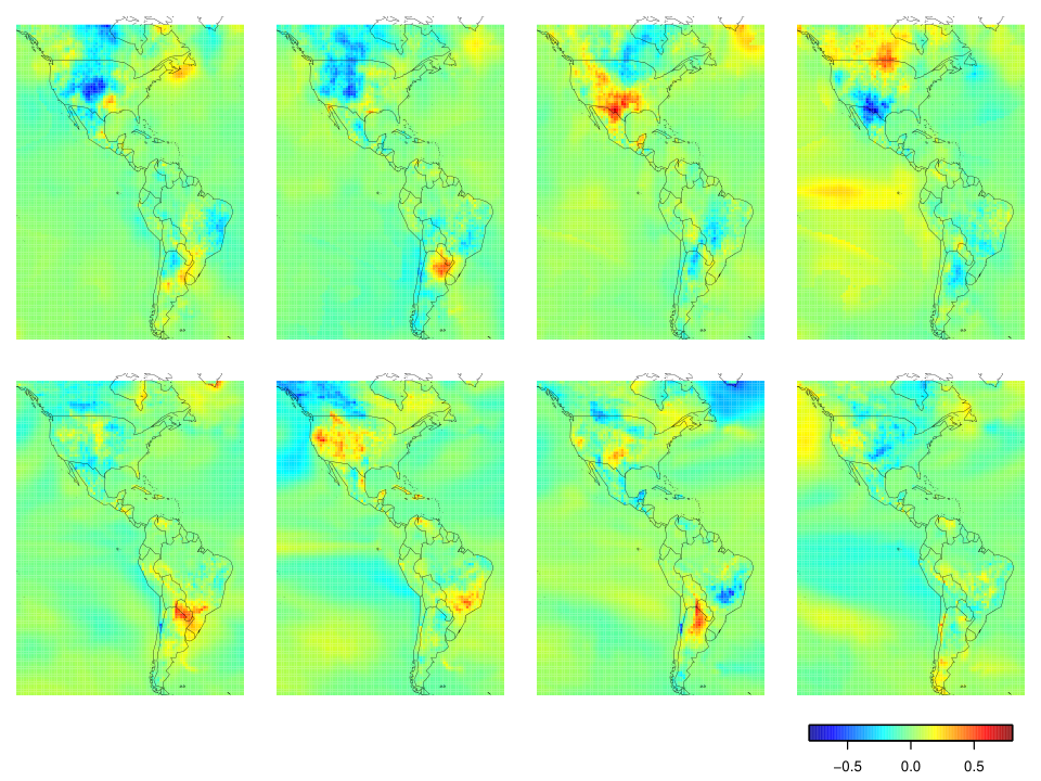
Figure 8 shows four realizations of the LK process on the top row, and for reference the first four ensemble members from the spatial data set are given on the bottom row. Qualitatively the spatial coherence and variability matches between these simulated and true cases. We note the emulation does have some modest deficiencies. For example, the anisotropy over the Equitorial Pacific is not well represented. In the model appears to be longer correlation scales in the East-West direction as compared to the North-South. Of course, this is not a failing of the LK approximation but rather the use of an isotropic covariance function. As a contrast to the non-stationary model we also generated stationary realizations. The top row of Figure 9 gives four realizations of a stationary field using the median of the parameter estimates over land. The bottom row is the same except the medians over the ocean are used. The similarity between top and bottom plot is deliberate; to aid in this comparison we use the white noise vectors for generating the land and ocean field in each column. The differences between these two choices of stationary models are striking and it is clear that neither would provide an accurate emulation of the model output.
4.3 Parallel implementation
This example was computed using a parallel strategy and the R language [26]. Fitting the spatial model for each window is an embarrassingly parallel operation and moreover the ensemble data set fields are relatively small (about 12Mb). We took the approach of using a supervisor R session and then spawning many R worker sessions. The supervisor session assigns tasks (i.e. specific local windows) to each worker based on balancing the work load. When a worker is done with a specific task the information from the fitting is passed back the supervisor. The complete set of results are assembled as an output list in the supervisor session and in our case this output list has as many components as grid boxes in the spatial domain and each contains the results of the local fitting. Creating the workers, broadcasting the spatial data set, and assigning the tasks is all done in R through the Rmpi package [27]. In using R we have leveaged the stable and rich set of spatial analysis tools that are available to the community. In particular the maximum likelihood estimates are found using the spatialProcess function from the fields package and is called in exactly the same way as on a laptop. We have used this approach on the NCAR supercomputer Cheyenne [3] and found it exhibits excellent (strong) scaling. An example of timing is given below in Figure 10. In this test case a one level LK model limited to a 1000 grid boxes is fit directly to the data rather than the Matérn covariance. Here we see linear scaling in the time with up to 1000 parallel R worker sessions. As expected the time to spawn workers shows a linear increase (orange points) but is an order of magnitude smaller that the time spent in computation (blue points). Note that this scaling has attractive practical implications. Using 1000 cores will result in nearly a factor of 1000 speedup in the analysis and can potentially convert a lengthly batch analysis into one that is almost interactive.
5 Discussion
Combining local covariance estimation with a global model provides a practical route for modeling and simulating large spatial data sets. We have shown that the LK model can reproduce abrupt non-stationarity in a process where the range parameter has a discontinuity and as expected does well when the range parameter varies smoothly across a spatial domain. Moreover, in places where the process is locally stationary we see that there is close agreement between the Matèrn correlation function and the approximate one from the LK representation. The advantage of the LK representation is the ability to generate unconditional realization of the process at large number of locations. One can also use the LK model for spatial prediction and inference [12] although that role is not needed for climate model emulation.
Most data analysis represents a compromise between model complexity and realism and the need to estimate the model accurately from data. In this work we focused on data that has spatial replicates and this makes parameter estimation much more stable. In addition we do not believe this data set to be an isolated example as ensemble climate experiments are now the norm in climate science. The local covariance models could be improved by adding anisotropy and also covariates for the land/ocean regions. Because the LK likelihood can be evaluated for the complete data set, there is the opportunity to fit parameters that have a global extent, such as land/ocean effects, along with local covariance parameters. Some parameters such as anisotropy could also have larger spatial extent in order to provide stable estimate. The estimation strategy in this case would have the flavor of back-fitting in additive models where one would alternate between fitting different components of the model until convergence is obtained.
Local covariance fitting has the advantage that it leverages standard spatial tools and diagnostics. A more comprehensive approach would be to fit the fields of parameter maximizing the complete likelihood. To this end the local estimates could be used as the initial values in a LK model and subsequent optimization can refine these parameters. Recent work in deep learning has benefited from the use of stochastic gradient descent for fitting many parameters in an artificial neural network and this technique may also be useful for optimizing the parameters here.
From an analytical perspective it would be useful to determine the differences between the explicit non-stationary models following Paciorek’s construction and those derived via process convolution. Preliminary results, not reported here, suggest that these models are substantially different for the case of a discontinuity in the range parameter. In general we have found a process based description to be more fruitful for arriving at covariance models. For example, we build connection weights in a SAR model rather than the more general MRF framework. There is an additional benefit from process models that they can admit physical interpretation and be more useful to domain scientists.
The use of embarrassingly parallel steps, such as local covariance fitting or local simulation, is a computational strategy that merits more attention. Here we have developed code mainly in R to manage this process and so this framework is accessible to any accomplished R user. Indeed, the framework we use on the supercomputing system is the same that we use on a laptop except for several lines of batch scripting and changing directory pathnames. We also believe that this style of computation may drive alternative models and algorithms as the number of processors/cores available for routine spatial data analysis grows.
Acknowledgements
This work was supported in part by the National Center for Atmospheric Research (NCAR) and also the National Science Foundation Award 1406536. NCAR is sponsored by the National Science Foundation and managed by the University Corporation for Atmospheric Research. We also acknowledge high-performance computing support from Cheyenne (doi:10.5065/D6RX99HX) provided by NCAR’s Computational and Information Systems Laboratory, sponsored by the National Science Foundation.
Appendix A Wendland radial basis kernel
The Wendland functions are compacted supported on and are also positive definite. Below is the version of the Wendland valid up to 3 dimensions and belonging to :
Appendix B Normalization to approximate stationarity
Because of the discrete nature of the SAR the marginal variance of the LatticeKrig process will not be constant in the spatial domain. This can cause artifacts in the estimated surface and compromised its ability to approximate stationary covariance functions. To adjust the marginal variances we compute the unnormalized variance and divide by this quantity to give a constant variance at any location.
Based on the model and notation from Section 3, let and at multi-resolution level ,
Accordingly, let and normalize the basis functions as
These are the actual basis functions used in the spatial analysis.
References
- [1] Stacey E Alexeeff, Doug Nychka, Stephan R Sain, and Claudia Tebaldi. Emulating mean patterns and variability of temperature across and within scenarios in anthropogenic climate change experiments. Climatic Change, pages 1–15, 2016.
- [2] Ethan Anderes and Michael Stein. Local likelihood estimation for nonstationary random fields. Journal of Multivariate Analysis, 2011.
- [3] Computational and Information Systems Laboratory. Cheyenne: SGI ICE XA System (Climate Simulation Laboratory). National Center for Atmospheric Research, Boulder, Colorado, USA, 2017.
- [4] Noel Cressie and Gardar Johannesson. Fixed rank kriging for very large spatial data sets. Journal of the Royal Statistical Society: Series B (Statistical Methodology), 70(1):209–226, 2008.
- [5] Abhirup Datta, Sudipto Banerjee, Andrew O Finley, and Alan E Gelfand. Hierarchical nearest-neighbor gaussian process models for large geostatistical datasets. Journal of the American Statistical Association, 111(514):800–812, 2016.
- [6] Douglas Nychka, Reinhard Furrer, John Paige, and Stephan Sain. fields: Tools for spatial data, 2017. R package version 9.3.
- [7] Francky Fouedjio, Nicolas Desassis, and Jacques Rivoirard. A generalized convolution model and estimation for non-stationary random functions. Spatial Statistics, 16:35–52, 2016.
- [8] Montserrat Fuentes. Spectral methods for nonstationary spatial processes. Biometrika, 89(1):197–210, 2002.
- [9] Geir-Arne Fuglstad, Daniel Simpson, Finn Lindgren, and Håvard Rue. Exploring a new class of non-stationary spatial gaussian random fields with varying local anisotropy. Statistica Sinica, 25(1):115–133, 2015.
- [10] Timothy C Haas. Kriging and automated variogram modeling within a moving window. Atmospheric Environment. Part A. General Topics, 24(7):1759–1769, 1990.
- [11] Timothy C. Haas. Lognormal and moving window methods of estimating acid deposition. Journal of the American Statistical Association, 85(412):950–963, 1990.
- [12] Matthew J Heaton, Abhirup Datta, Andrew Finley, Reinhard Furrer, Rajarshi Guhaniyogi, Florian Gerber, Robert B Gramacy, Dorit Hammerling, Matthias Katzfuss, Finn Lindgren, et al. Methods for analyzing large spatial data: A review and comparison. arXiv preprint arXiv:1710.05013, 2017.
- [13] Dave Higdon et al. Space and space-time modeling using process convolutions. Quantitative methods for current environmental issues, 3754:37–56, 2002.
- [14] David Higdon. A process-convolution approach to modelling temperatures in the north atlantic ocean. Environmental and Ecological Statistics, 5(2):173–190, 1998.
- [15] Jay M. Ver Hoef, Noel Cressie, and Ronald Paul Barry. Flexible spatial models for kriging and cokriging using moving averages and the fast fourier transform (fft). Journal of Computational and Graphical Statistics, 13(2):265–282, 2004.
- [16] Matthias Katzfuss. A multi-resolution approximation for massive spatial datasets. Journal of the American Statistical Association, 112(517):201–214, 2017.
- [17] Matthias Katzfuss and Noel Cressie. Spatio-temporal smoothing and em estimation for massive remote-sensing data sets. Journal of Time Series Analysis, 32(4):430–446, 2011.
- [18] JE Kay, C Deser, A Phillips, A Mai, C Hannay, G Strand, JM Arblaster, SC Bates, G Danabasoglu, J Edwards, et al. The community earth system model (cesm) large ensemble project: A community resource for studying climate change in the presence of internal climate variability. Bulletin of the American Meteorological Society, 96(8):1333–1349, 2015.
- [19] Finn Lindgren, Håvard Rue, and Johan Lindström. An explicit link between gaussian fields and gaussian markov random fields: the stochastic partial differential equation approach. Journal of the Royal Statistical Society: Series B (Statistical Methodology), 73(4):423–498, 2011.
- [20] Finn Lindgren and Håvard Rue. Explicit construction of gmrf approximations to generalised matérn fields on irregular grids. Technical report, [Publisher information missing], 2007.
- [21] Douglas Nychka, Soutir Bandyopadhyay, Dorit Hammerling, Finn Lindgren, and Stephan Sain. A multiresolution gaussian process model for the analysis of large spatial datasets. Journal of Computational and Graphical Statistics, 24(2):579–599, 2015.
- [22] Douglas Nychka, Dorit Hammerling, Stephan Sain, and Nathan Lenssen. Latticekrig: Multiresolution kriging based on markov random fields, 2016. R package version 6.6.
- [23] Christopher J Paciorek and Mark J Schervish. Spatial modelling using a new class of nonstationary covariance functions. Environmetrics, 17(5):483–506, 2006.
- [24] Michael L Stein. Nonstationary spatial covariance functions. Unpublished technical report, 2005.
- [25] Michael L Stein, Zhiyi Chi, and Leah J Welty. Approximating likelihoods for large spatial data sets. Journal of the Royal Statistical Society: Series B (Statistical Methodology), 66(2):275–296, 2004.
- [26] R Core Team. R language definition. Vienna, Austria: R foundation for statistical computing, 2000.
- [27] Hao Yu. Rmpi: Parallel statistical computing in r. R News, 2(2):10–14, 2002.
- [28] Zhengyuan Zhu and Yichao Wu. Estimation and prediction of a class of convolution-based spatial nonstationary models for large spatial data. Journal of Computational and Graphical Statistics, 19(1):74–95, 2010.
Figures