High Order Finite Difference Schemes for the Heat Equation Whose Convergence Rates are Higher Than Their Truncation Errors^1,2

Consider the differential problem:

	$\displaystyle\frac{\partial\,u}{\partial t}$	$\displaystyle=$	$\displaystyle P\left(\frac{\partial\,}{\partial x}\right)u\;\;,\;\;\;\;\;x\in\Omega\subset{\mathbb{R}}^{d}\;,t\geq 0$
	$\displaystyle u(t=0)$	$\displaystyle=$	$\displaystyle f(x)\;.$

where $u=(u_{1},\ldots,u_{m})^{T}$ and $P\left({\partial\,}/{\partial x}\right)$ is a linear differential operator with appropriate boundary conditions. It is assumed that this problem is well posed, i.e. $\exists K(t)<\infty$ such that $||u(t)||\leq K(t)||f||$, where typically $K(t)=Ke^{\alpha t}$.

Let $Q$ be the discretization of $P\left(\partial\,/\partial x\right)$ where we assume:

Assumption 1:

The discrete operator $Q$ is based on grid points $\{x_{j}\}$, $j=1,\ldots,N$.

Assumption 2:

$Q$ is semi–bounded in some equivalent scalar product $\left(\cdot,\cdot\right)_{H}=\left(\cdot,H\cdot\right)$, i.e

$$\left({{\bf w}},Q{{\bf w}}\right)_{H}\,\leq\,\alpha\left({{\bf w}},{{\bf w}}\right)_{H}\,=\,\alpha\left\|{{\bf w}}\right\|_{H}^{2}\;.$$

(2)

Assumption 3:

The local truncation error vector of $Q$ is ${{\bf T}}_{e}$ which is defined, at each entry $j$ by

$$\left({{\bf T}}_{e}\right)_{j}\,=\,\left(Pw(x_{j})\right)\,-\,\left(Q{{\bf w}}\right)_{j},$$

(3)

where $w(x)$ is a smooth function and ${{\bf w}}$ is the projection of $w(x)$ onto the grid. It is assumed that $\left\|{{\bf T}}_{e}\right\|\xrightarrow{N\rightarrow\infty}0$.

Consider the semi–discrete approximation:

	$\displaystyle\frac{\partial\,{{\bf v}}}{\partial t}$	$\displaystyle=$	$\displaystyle Q{{\bf v}}\;\;,\;\;\;\;\;t\geq 0$		(4)
	$\displaystyle{{\bf v}}(t=0)$	$\displaystyle=$	$\displaystyle{{\bf f}}\;.$

Proposition: Under Assumptions 1–3 The semi–discrete approximation converges.
Proof: Let ${{\bf u}}$ is the projection of $u(x,t)$ onto the grid. Then, from assumption 3,

$$\frac{\partial\,{{\bf u}}}{\partial t}\,=\,P{{\bf u}}\,=\,Q{{\bf u}}+{{\bf T}}_{e}\;.$$

(5)

Let ${{\bf E}}={{\bf u}}-{{\bf v}}$ then by subtracting (4) from (5) one obtains the equation for ${{\bf E}}$, namely

$$\frac{\partial\,{{\bf E}}}{\partial t}\,=\,Q{{\bf E}}+{{\bf T}}_{e}\;.$$

(6)

Next, by taking the $H$ scalar product with ${{\bf E}}$, using assumption 2 and the Schwartz inequality the following estimate can be derived

$$\left({{\bf E}},\frac{\partial\,{{\bf E}}}{\partial t}\right)_{H}\;=\;\frac{1}{2}\frac{\partial\,}{\partial t}\left({{\bf E}},{{\bf E}}\right)_{H}\;=\;\left\|{{\bf E}}\right\|_{H}\frac{\partial\,}{\partial t}\left||{{\bf E}}\right\|_{H}\;=\;\left({{\bf E}},Q{{\bf E}}\right)_{H}+\left({{\bf E}},{{\bf T}}_{e}\right)_{H}\;\\ \;\leq\;\alpha\left({{\bf E}},{{\bf E}}\right)_{H}\,+\,\left\|{{\bf E}}\right\|_{H}\left\|{{\bf T}}_{e}\right\|_{H}\;.$$

Thus

$$\frac{\partial}{\partial t}\left\|{{\bf E}}\right\|_{H}\,\leq\,\alpha\left\|{{\bf E}}\right\|_{H}+\left\|{{\bf T}}_{e}\right\|_{H}\;.$$

(7)

Therefore:

$$\left\|{{\bf E}}\right\|_{H}(t)\,\leq\,\left\|{{\bf E}}\right\|_{H}(t=0){\rm e}^{\alpha t}+\frac{{\rm e}^{\alpha t}-1}{\alpha}\max_{0\leq\tau\leq t}\left\|{{\bf T}}_{e}\right\|_{H}\;\xrightarrow{N\rightarrow\infty}\;0\;.$$

(8)

Here we assumed that $\left\|{{\bf E}}\right\|_{H}(t=0)$ is either 0, or at least of the order of machine accuracy. Equation (8) establishes the fact that if the scheme is stable and consistent, the numerical solution ${{\bf v}}$ converges to the projection of the exact solution onto the grid, ${{\bf u}}$. Furthermore, it assures that the error will be at most in the truncation error $\left\|{{\bf T}}_{e}\right\|_{H}$. This is one part of the landmark Lax–Richtmyer equivalence theorem for semi–discrete approximation. See e.g. [6].

Due to this and similar results the common way for constructing finite difference schemes is to derive a semi–bounded $Q$ with proper truncation error. Typically the error $\left\|{{\bf E}}\right\|_{H}$ is indeed of the order of $\left\|{{\bf T}}_{e}\right\|_{H}$.

It should be noted, however, that (6) is the exact equation for the error dynamics, while (8) is an estimate. In this paper we present finite difference schemes in which the errors are smaller than their truncation errors. It is well known that boundary conditions can be of one order lower accuracy without destroying the convergence rate expected from the approximation at inner points, see e.g. [4], [5], [1] and [10]. In [5] and [10] it was shown that for parabolic, incompletely parabolic and 2nd-order hyperbolic equations the boundary conditions can be of two order less. Here, however, we consider low order truncation errors in most or all of the grid points.

This paper is constructed as follows; in Section 2 we present a preliminary example and illustrate the mechanism which reduces the error. In Section 3 we present a two–point block scheme which has a first order truncation error but has a second or third order error. In Section 4 two three–point block schemes are presented. Discussion and remarks are presented in Section 5.

Consider the heat equation

	$\displaystyle\frac{\partial\,u}{\partial t}$	$\displaystyle=$	$\displaystyle\frac{\partial^{2}\,u}{\partial x^{2}}+F(x,t)\;\;,\;\;\;\;\;x\in[0,2\pi)\;,t\geq 0$
	$\displaystyle u(t=0)$	$\displaystyle=$	$\displaystyle f(x)$		(9)

with periodic boundary conditions.
Let the scheme be:

	$\displaystyle\frac{\partial\,v_{j}}{\partial t}$	$\displaystyle=$	$\displaystyle D_{+}D_{-}v_{j}\,+\,(-1)^{j}\,c\,v_{j}\,+\,F_{j}(t)\;\;;\;\;\;\;\;x_{j}=jh,\;\;h=2\pi/N\;,\;\;N\;{\rm is\;even}$
	$\displaystyle v_{j}(t=0)$	$\displaystyle=$	$\displaystyle f_{j}$		(10)

where $F_{j}(t)$ is the projection of $F(x,t)$ onto the spatial grid. The truncation error is

$$\left(T_{e}\right)_{j}=\frac{h^{2}}{12}\left(u_{j}\right)_{xxxx}+O(h^{2})-(-1)^{j}\,c\,v_{j}=O(1)\;.$$

(11)

Formally, this scheme is not consistent. The scheme (10) was run with the initial condition $f(x)\,=\,\cos(x)$, $F=0$ and $N=32,64,\ldots,1024$ with forward–Euler time propagator. The plots of $\log_{10}\|{{\bf E}}\|$ vs. $\log_{10}N$, at $t_{\rm final}=2\pi$, for $c=0,0.5,1$ are presented in Figure 1a. It can be seen that this is a second order scheme.

In order to understand this phenomenon let us consider one high frequency mode of the error³³ 3 This scheme was presented for demonstrating the phenomenon that the error, due to high frequency modes, is lower than the truncation error. As this is not a practical scheme, full analysis of the error is not presented, only a demonstration of the dynamics of high frequency error modes is presented. Full analysis is given for the scheme presented in the next section. Denote $\left(T_{c}\right)_{j}=(-1)^{j}\,c\,v_{j}$. This term can also be written as:

$$\left(T_{c}\right)_{j}\,=\,(-1)^{j}\,c\,h^{\alpha}\,=\,ch^{\alpha}\,{\rm e}^{iNx_{j}/2}$$

(12)

For the scheme (10) $\alpha=0$. The equation for the error term caused by $T_{c}$ is

$$\frac{\partial\,{{\bf E}}_{c}}{\partial t}\,=\,D_{+}D_{-}{{\bf E}}_{c}+{{\bf T}}_{c}$$

(13)

Since $\left({{\bf E}}_{c}\right)_{j}=\hat{{{\bf E}}}_{c}\,{\rm e}^{iNx_{j}/2}\sqrt{2\pi}$, $\hat{{{\bf E}}}_{c}\in\mathbb{C}$, then the equation for $\hat{{{\bf E}}}_{c}$ is

$$\frac{\partial\,\hat{{{\bf E}}}_{c}}{\partial t}\,=\,-\left(\frac{N}{2}\right)^{2}\widehat{{{\bf E}}}_{c}+c^{\prime}h^{\alpha}$$

(14)

Therefore,

	$\displaystyle\left\|{{{\bf E}}}_{c}\right\|(t)\,=\,\left|\hat{{{\bf E}}}_{c}\right|(t)$	$\displaystyle=$	$\displaystyle\left|\hat{{{\bf E}}}_{c}\right|(0){\rm e}^{-\left(\frac{N}{2}\right)^{2}t}+\left(\frac{2}{N}\right)^{2}\left(1-{\rm e}^{-\left(\frac{N}{2}\right)^{2}t}\right)c^{\prime}h^{\alpha}$		(15)
		$\displaystyle\leq$	$\displaystyle\left|\hat{{{\bf E}}}_{c}\right|(0){\rm e}^{-\left(\frac{N}{2}\right)^{2}t}+O\left({h^{\alpha+2}}\right)$

Note that the actual error, $\left\|{{{\bf E}}}_{c}\right\|(t)$, is two orders lower that the truncation error, $\|T_{c}\|$. In the next sections we present practical schemes which utilize this idea.

Let the grid be: $x_{j}=j\,h$, $h=2\pi/(N+1)$ and $x_{j+1/2}=x_{j}+h/2$, $j=0,\ldots N$. Altogether there are $2(N+1)$ points with spacing of $h/2$. For simplicity, we assume that $N$ is even.

Consider the approximation:

	$\displaystyle\frac{d^{2}}{dx^{2}}u_{j}$	$\displaystyle\approx$	$\displaystyle\frac{1}{(h/2)^{2}}\left[\left(u_{j-1/2}-2u_{j}+u_{j+1/2}\right)\,+\,c\left(-u_{j-1/2}+3u_{j}-3u_{j+1/2}+u_{j+1}\right)\right]$
	$\displaystyle\frac{d^{2}}{dx^{2}}u_{{j+1/2}}$	$\displaystyle\approx$	$\displaystyle\frac{1}{(h/2)^{2}}\left[\left(u_{j}-2u_{j+1/2}+u_{j+1}\right)\,+\,c\left(u_{j-1/2}-3u_{j}+3u_{j+1/2}-u_{j+1}\right)\right]$

The truncation errors are:

	$\displaystyle\left(T_{e}\right)_{j}\hskip-5.69046pt$	$\displaystyle\;=\;$	$\displaystyle\hskip-5.69046pt\frac{1}{12}\left(\frac{h}{2}\right)^{2}\left(u_{j}\right)_{xxxx}+c\left[\left(\frac{h}{2}\right)\left(u_{j}\right)_{xxx}+\frac{1}{2}\left(\frac{h}{2}\right)^{2}\left(u_{j}\right)_{xxxx}\right]+O(h^{3})=O(h)$
	$\displaystyle\left(T_{e}\right)_{j+\frac{1}{2}}\hskip-5.69046pt$	$\displaystyle\;=\;$	$\displaystyle\hskip-5.69046pt\frac{1}{12}\left(\frac{h}{2}\right)^{2}\left(u_{j+\frac{1}{2}}\right)_{xxxx}+c\left[-\left(\frac{h}{2}\right)\left(u_{j+\frac{1}{2}}\right)_{xxx}+\frac{1}{2}\left(\frac{h}{2}\right)^{2}\left(u_{j+\frac{1}{2}}\right)_{xxxx}\right]+O(h^{3})=O(h)$

The motivation leading to this scheme is that the highly oscillating $O(h)$ error terms will be dissipated, as in the previous example, while the $O(h^{2})$ terms will be canceled, for the proper value of $c$.

In this section we briefly present two schemes which are based on three–point block. Here we use the grid, $x_{j}=j\,h$, $h=2\pi/(N+1)$ with the internal block nodes $x_{j+1/3}=x_{j}+h/3$ and $x_{j+2/3}=x_{j}+2h/3$, $j=0,\ldots N$. Altogether there are $3(N+1)$ points with spacing of $h/3$.

three–point block, 3rd order scheme

Consider the approximation:

	$\displaystyle\frac{d^{2}}{dx^{2}}u_{j}$	$\displaystyle=$	$\displaystyle\frac{1}{4(h/3)^{2}}\left[\left(4u_{j-1/3}-8u_{j}+4u_{j+1/3}\right)\,+\,c\left(-u_{j-1/3}+3u_{j}-3u_{j+1/3}+u_{j+2/3}\right)\right]\,+\,O(h)$
	$\displaystyle\frac{d^{2}}{dx^{2}}u_{j+1/3}$	$\displaystyle=$	$\displaystyle\frac{1}{4(h/3)^{2}}\left[\left(4u_{j}-8u_{j+1/3}+4u_{j+2/3}\right)\right]\,+\,O(h^{2})$		(33)
	$\displaystyle\frac{d^{2}}{dx^{2}}u_{{j+2/3}}$	$\displaystyle=$	$\displaystyle\frac{1}{4(h/3)^{2}}\left[\left(4u_{j+1/3}-8u_{j+2/3}+4u_{j+1}\right)\,+\,c\left(u_{j}-3u_{j+1/3}+3u_{j+2/3}-u_{j+1}\right)\right]\,+\,O(h)$

This scheme was run under the same conditions as the example in Section 3. As in the previous example the truncation error is of $O(h)$, however this is a 2nd order scheme and 3rd order for $c=1.340$. The convergence results are presented in Figure 2a.

three–point block, 5th order scheme

	$\displaystyle\frac{d^{2}}{dx^{2}}u_{j}$	$\displaystyle=$	$\displaystyle\frac{1}{12(h/3)^{2}}\left[\left(-u_{j-2/3}+16u_{j-1/3}-30u_{j}+16u_{j+1/3}-u_{j+2/3}\right)\,+\,\right.$
			$\displaystyle\left.c\left(u_{j-2/3}-5u_{j-1/3}+10u_{j}-10u_{j+1/3}+5u_{j+2/3}-u_{j}\right)\right]\,+\,O(h^{3})$
	$\displaystyle\frac{d^{2}}{dx^{2}}u_{j+1/3}$	$\displaystyle=$	$\displaystyle\frac{1}{12(h/3)^{2}}\left[\left(-u_{j-1/3}+16u_{j}-30u_{j+1/3}+16u_{j+2/3}-u_{j}\right)\right]\,+\,O(h^{4})$		(34)
	$\displaystyle\frac{d^{2}}{dx^{2}}u_{{j+2/3}}$	$\displaystyle=$	$\displaystyle\frac{1}{12(h/3)^{2}}\left[\left(-u_{j}+16u_{j+1/3}-30u_{j+2/3}+16u_{j+1}-u_{j+4/3}\right)\,+\,\right.$
			$\displaystyle\left.c\left(-u_{j-1/3}+5u_{j}-10u_{j+1/3}+10u_{j+2/3}-5u_{j+1}+u_{j+4/3}\right)\right]\,+\,O(h^{3})$

This scheme was run under the same conditions as the previous examples, with the exception that now a 6th order Runge–Kutta scheme was used for time integration. Here the truncation error is of $O(h^{3})$, however this is a 4th order scheme and 5th order for $c=-0.385$. The convergence results are presented in Figure 2b.

It should be noted that by taking $c=1$ the coefficients of $u_{j-2/3}$ and $u_{j+4/3}$ are 0. Therefore the scheme is more ’compact’ than standard explicit 4th order scheme in the sense that the scheme depends only on one term, on each side, out of the three–point block $u_{j},u_{j+1/3},u_{j+2/3}$. Potentially, this thinner stencil helps in the derivation of boundary schemes for initial–boundary value problems.

In this paper we presented a few block–finite–difference schemes in which the actual errors are much smaller than their truncation errors. This reduction of error was achieved by constructing the truncation errors to be oscillatory and using the dissipative property of the scheme.

A comparison between standard and block finite difference schemes in terms of the number of points out of the cell and operation count is presented in Table 1. As can be seen, in terms of accuracy and computational cost the 3rd and 5th order schemes are between the standards 2nd and 4th order and 4th and 6th order schemes respectively.

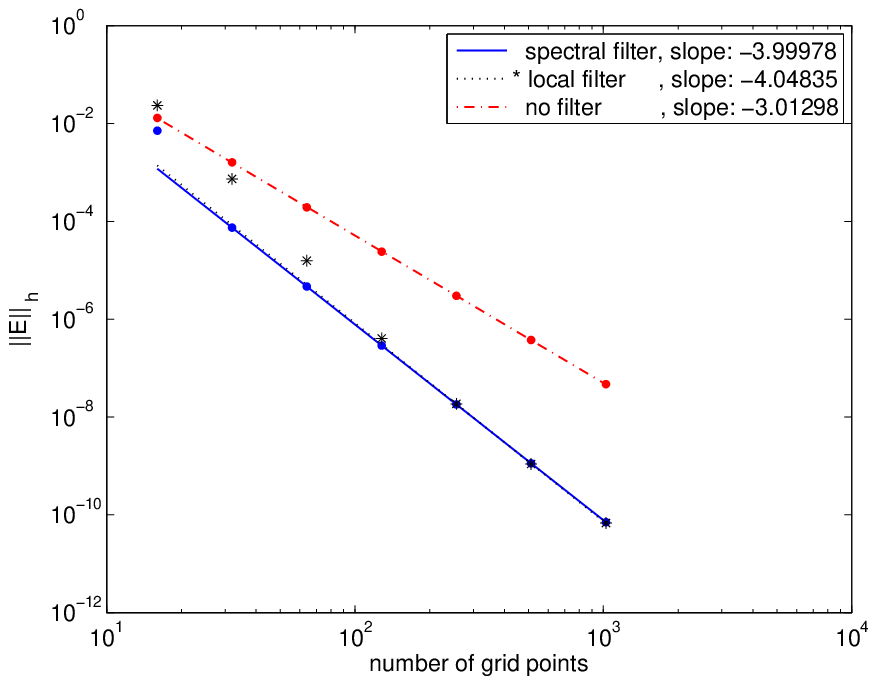
If $c=-1/4$ in the two–point block, 3rd order scheme (3), the leading term in the error is highly oscillatory, see (32). It was suggested by Jennifer K. Ryan [8] that this term can be filtered by post–processing. In this technique the high frequency error terms are filtered using convolution with a proper kernel. This method was successfully applied to the discontinuous Galerkin method. As this filtering is done only once, after the final time step, the cost is minimal, see e.g. [9], [2], [3]. Here we used a global spectral filter and the local filter suggested in [3]. As can be seen in figure 3, the filtered scheme is 4th order accurate. The difference between both kernels is that the global filter is more computationally expensive, $O(N\,\log N)$ for proper values of $N$, but is accurate for small values of $N$ while the local filter requires only $O(N)$ operation but is accurate only for large values of $N$. The investigation of which is the optimal filter for these schemes is a topic for future research.

It should be noted that that finite difference representations of discontinuous Galerkin schemes for the heat equation have a similar form to the schemes presented above. They may also present similar enhancing of accuracy. See [11]. This manuscript was the inspiration to the current work. As was also pointed out in [11] the increasing of accuracy may be related to a phenomenon called Supra–Convergence [7].

Further research of the properties and implementations of these schemes as well as the existence of these kinds of schemes for hyperbolic problems are topics for future research.

Acknowledgments
The author would like to thank Jennifer K. Ryan, Chi–Wang Shu and Sigal Gottlieb for the fruitful discussions and their help. The author would also like to thank the anonymous reviewers for their useful remarks.

References

• (1) Saul Abarbanel, Adi Ditkowski, and Bertil Gustafsson, On error bounds of finite difference approximations to partial differential equations—temporal behavior and rate of convergence, Journal of Scientific Computing 15 (2000), no. 1, 79–116.
• (2) Bernardo Cockburn, Mitchell Luskin, Chi-Wang Shu, and Endre Suli, Post-processing of galerkin methods for hyperbolic problems, Springer, 2000.
• (3)   , Enhanced accuracy by post-processing for finite element methods for hyperbolic equations, Mathematics of Computation 72 (2003), no. 242, 577–606.
• (4) Bertil Gustafsson, The convergence rate for difference approximations to mixed initial boundary value problems, Mathematics of Computation 29 (1975), no. 130, 396–406.
• (5)   , The convergence rate for difference approximations to general mixed initial-boundary value problems, SIAM Journal on Numerical Analysis 18 (1981), no. 2, 179–190.
• (6) Bertil Gustafsson, Heinz-Otto Kreiss, and Joseph Oliger, Time-dependent problems and difference methods, John Wiley & Sons, 1995.
• (7) H-O Kreiss, Thomas A Manteuffel, B Swartz, B Wendroff, and AB White, Supra-convergent schemes on irregular grids, Mathematics of Computation 47 (1986), no. 176, 537–554.
• (8) Jennifer Ryan, Privet communucation.
• (9) Jennifer Ryan, Chi-Wang Shu, and Harold Atkins, Extension of a post processing technique for the discontinuous galerkin method for hyperbolic equations with application to an aeroacoustic problem, SIAM Journal on Scientific Computing 26 (2005), no. 3, 821–843.
• (10) Magnus Svärd and Jan Nordström, On the order of accuracy for difference approximations of initial-boundary value problems, Journal of Computational Physics 218 (2006), no. 1, 333–352.
• (11) Mengping Zhang and Chi-Wang Shu, An analysis of three different formulations of the discontinuous galerkin method for diffusion equations, Mathematical Models and Methods in Applied Sciences 13 (2003), no. 03, 395–413.