Residual Parameter Transfer for Deep Domain Adaptation

Artem Rozantsev Mathieu Salzmann Pascal Fua Affiliation: Computer Vision Laboratory, École Polytechnique Fédérale de Lausanne Affiliation: Lausanne, Switzerland Email: {firstname.lastname}@epfl.ch

Abstract

The goal of Deep Domain Adaptation is to make it possible to use Deep Nets trained in one domain where there is enough annotated training data in another where there is little or none. Most current approaches have focused on learning feature representations that are invariant to the changes that occur when going from one domain to the other, which means using the same network parameters in both domains. While some recent algorithms explicitly model the changes by adapting the network parameters, they either severely restrict the possible domain changes, or significantly increase the number of model parameters.

By contrast, we introduce a network architecture that includes auxiliary residual networks, which we train to predict the parameters in the domain with little annotated data from those in the other one. This architecture enables us to flexibly preserve the similarities between domains where they exist and model the differences when necessary. We demonstrate that our approach yields higher accuracy than state-of-the-art methods without undue complexity.

1 Introduction

Given enough training data, Deep Neural Networks [1, 2] have proven extremely powerful. However, there are many situations where sufficiently large training databases are difficult or even impossible to obtain. In such cases, Domain Adaptation [3] can be used to leverage annotated data from a source domain in which it is plentiful to help learn the network parameters in a target domain in which there is little, or even no, annotated data.

The simplest approach to Domain Adaptation is to use the available annotated data in the target domain to fine-tune a Convolutional Neural Network (CNN) pre-trained on the source data [4, 5]. However this can result in overfitting when too little labeled target data is available and is not applicable at all in the absence of any such labeled target data.

One way to overcome this problem is to design features that are invariant to the domain shift, that is, the differences between the statistics in the two domains. This is usually done by introducing loss terms that force the statistics of the features extracted from both domains to be similar [6, 7, 8, 9]. While effective when the domain shift is due to lighting or environmental changes, enforcing this kind of statistical invariance may discard information and negatively impact performance.

Refer to caption — Figure 1: Our two-stream architecture. One stream operates on the source data and the other on the target one. Their parameters are not shared. Instead, we introduce a residual transformation network that relates the parameters of the streams with each other.

To overcome this, it has been proposed to explicitly model the domain shift [10, 11]. In particular, the method in [10] involves learning private and shared encoders for each of the domains, which increases the number of parameters to be learned by a factor of $4$ . By contrast, the approach in [11] relies on a two-stream architecture with related but non-shared parameters to model the shift. This only require a $2$ -fold increase in the number of parameters to be learned but at the cost of restricting corresponding parameters in the two domains to approximately be scaled and shifted versions of each other. Furthermore, it requires selecting the layers that have non-shared parameters using a validation procedure that does not scale up to modern very deep architectures such as those of [12, 13].

In this paper, we also explicitly model the domain shift between the two domains using a two-stream architecture with non-shared parameters. However, we allow for a much broader range of transformations between the parameters in both streams and automatically determine during training how strongly related corresponding layers should be. As a result, our approach can be used in conjunction with very deep architectures.

Specifically, we start from a network trained on the source data and fine-tune it while learning additional auxiliary, residual networks that adapt the layer parameters to make the final target feature distribution as close as possible to the final distribution of the source features. Furthermore, we regularize the capacity of these auxiliary networks by finding an optimal rank for their parameter matrices, and thus learn the relationship between corresponding layers in the two streams. Our contribution therefore is twofold:

•

We model the domain shift by learning meta parameters that transform the weights and biases of each layer of the network. They are depicted by the horizontal branches in Fig. 1.
•

We propose an automated scheme to adapt the complexity of these transformations during learning.

This results in a performance increase compared to the approaches of [10] and [11], along with a reduction in the number of parameters to be learned by a factor $2.5$ and $1.5$ compared to the first and second, respectively. As demonstrated by our experiments, we also outperform the state-of-the-art methods that attempt to learn shift invariant features [8, 14].

2 Related Work

Most approaches to domain adaptation (DA) that operate on deep networks focus on learning features that are invariant to the domain shift [6, 7, 8, 9, 15, 16]. This is usually achieved by adding to the loss function used for training a term that forces the distributions of the features extracted from the source and target domains to be close to each other.

In [6], the additional loss term is the Maximum Mean Discrepancy (MMD) measure [17]. This was extended in [7] by using multiple MMD kernels to better model differences between the two domains. In [16], this was further extended by computing the loss function of [7] at multiple levels, including on the raw classifier output. The MMD measure [17] that underpins these approaches is based on first order statistics. This was later generalized to second-order statistics [18, 19] and to even higher-order ones [20].

In [8, 9, 21] a different approach was followed, involving training an additional classifier to predict from which domain a sample comes. These methods then aim to learn a feature representation that fools this classifier, or, in other words, that carries no information about the domain a sample belongs to. This adversarial approach eliminates the need to manually model the distance measure between the final source and target feature distributions and enables the network to learn it automatically.

While effective, all these methods aim to learn domain invariant features, with a single network shared by the source and target data. By contrast, in [22], a network pre-trained on the source domain was refined on the target data by minimizing the adversarial loss of [9] between the fixed source features and the trainable target representation. Furthermore, in [10], differences and similarities between the two domains are modeled separately using private and shared encoders that generate feature representations, which are then given to a reconstruction network. The intuition is that, by separating domain similarities and differences, the network preserves some information from the source data and learns the important properties of the target data. While effective, this quadruples the total number of model parameters, thus restricting the applicability of this approach to relatively small architectures. In the same spirit, the approach of [11] relies on a two-stream architecture, one devoted to each domain. Some layers do not share their parameters, which are instead encouraged to be scaled and shifted versions of each other. While effective, this severely restricts the potential transformations from one domain to the other. Furthermore, the subsets of layers that are shared or stream-specific are found using a validation procedure, which scales poorly to the very deep architectures that achieve state-of-the-art performance in many applications.

In this paper, we introduce a two-stream architecture that suffers from none of these limitations.

3 Approach

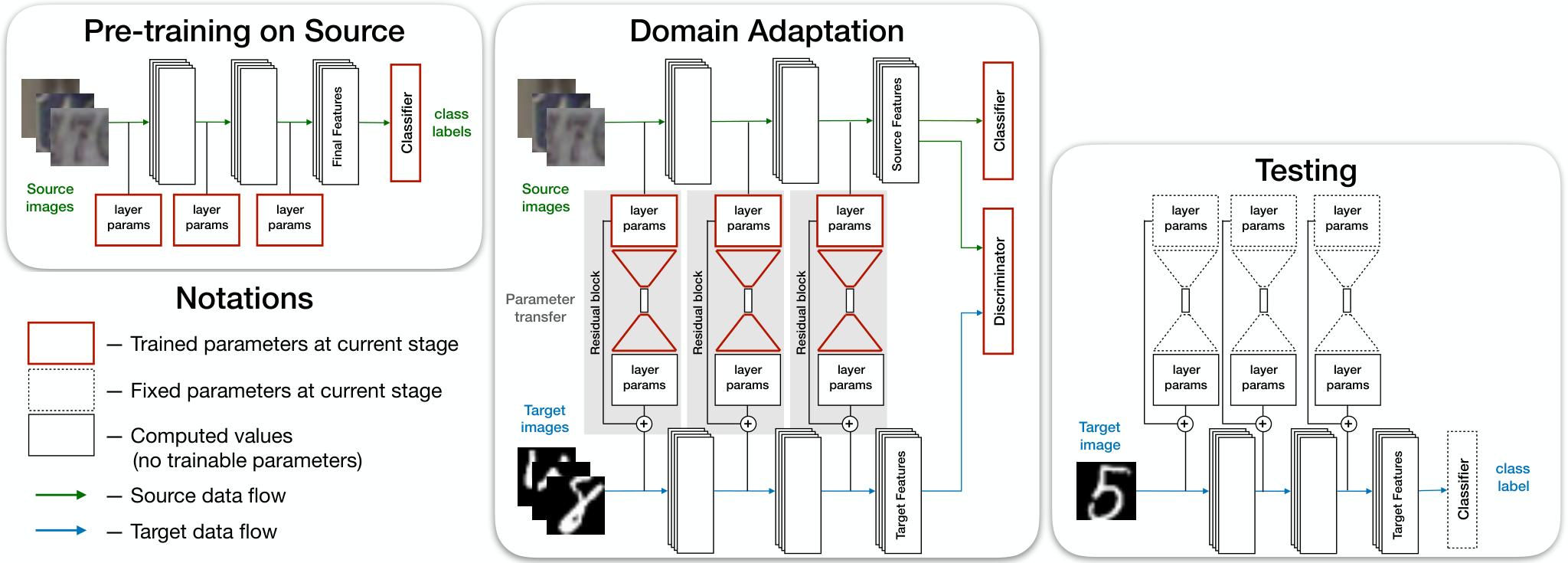
We start from an arbitrary network that has been trained on the source domain, which we refer to as source stream. We then introduce auxiliary networks that transform the source stream parameters to generate a target stream, as depicted by Fig. 1. We jointly train the auxiliary networks and refine the original source stream using annotated source data and either a small amount of annotated samples from the target domain or unlabeled target images only. We refer to the former as the supervised case and to the latter as the unsupervised one.

Fig. 2 summarizes our approach. Its Domain Adaptation component appears in the center, and we now describe it in detail. To this end, we first introduce our auxiliary networks and then show that we can control the rank of their weight matrices to limit the number of parameters that need to be learned. In effect, during training, our network automatically learns which layers should be different from each other and which ones can have similar or equal parameters.

3.1 Adapting the Parameters of Corresponding Layers

Let $\Omega$ be the set of all layers in a single stream of the Deep Network architecture illustrated in Fig. 1. For each layer $i\in\Omega$ , let us first consider a vector representation of the source and target stream parameters as $\theta_{i}^{s}$ and $\theta_{i}^{t}$ , respectively.

A natural way to transform the source parameters into the target ones is to write

\theta_{i}^{t}=\mathbf{B}_{i}\sigma(\mathbf{A}_{i}^{\intercal}\theta_{i}^{s}+\mathbf{d}_{i})+\theta_{i}^{s},\quad\forall i\in\Omega\;,

(1)

for which the notation is given in Table 1. Note that $k_{i}$ , the second dimension of the $\mathbf{A}_{i}$ and $\mathbf{B}_{i}$ matrices, controls the complexity of the transformation by limiting the rank of the matrices. $k_{i}=0$ corresponds to the degenerate case where the parameters of the source and target streams are identical, that is, shared between the two streams.

$\sigma(\cdot)$	$\in\{\tanh,\texttt{ReLU}\}$	nonlinear activation
$\mathbf{A}_{i},\mathbf{B}_{i}$	$\in\mathbb{R}^{M_{i}\times k_{i}}$	transformation matrices
$k_{i}$	$k_{i}\geq 0$	transformation rank
$\mathbf{d}_{i}$	$\in\mathbb{R}^{k_{i}}$	bias term
$M_{i}$	the number of parameters in the $i^{th}$ layer
$\Omega$	the set of all network layers

Table 1: Notation for Eq. 1.

In theory, we could learn all the coefficients of these matrices for all layers, along with their rank, by minimizing a loss function such as the one defined in Section 3.2. Unfortunately, the formulation of Eq. 1 results in a memory intensive implementation because each increase of the transformation rank $k_{i}$ by $1$ in any layer creates $(2M_{i}+1)$ additional parameters, which quickly becomes impractically large, especially when dealing with fully-connected layers.

To address this issue, we propose to rewrite the layer parameters in matrix form. Our strategy for different layer types is as follows:

•

Fully connected layer. Such a layer performs a transformation of the form $\mathbf{y}=\sigma(\mathbf{A}\mathbf{x}+\mathbf{b})$ , where $\mathbf{A}$ is a matrix and $\mathbf{b}$ a vector whose size is the number of rows of $\mathbf{A}$ . In this case, we simply concatenate $\mathbf{A}$ and $\mathbf{b}$ into a single matrix.
•

Convolutional layer. Such a layer is parametrized by a tensor $\mathbf{W}\in\mathbb{R}^{N_{out}\times N_{in}\times f_{x}\times f_{y}}$ , where the convolutional kernel is of size $f_{x}\times f_{y}$ , and a bias term $\mathbf{b}\in\mathbb{R}^{N_{out}}$ . We therefore represent all these parameters as a single matrix by reshaping the kernel weights as an $N_{out}\times N_{in}f_{x}f_{y}$ matrix and again concatenating the bias with it.

Following these operations, the parameters of each layer $i$ in the source and target streams are represented by matrices $\Theta_{i}^{s}$ and $\Theta_{i}^{t}$ , respectively. We then propose to write the transformation from the source to the target parameters as

\Theta_{i}^{t}=\mathbf{\mathcal{B}}_{i}^{1}\sigma\hskip-2.84544pt\left(\left(\mathbf{\mathcal{A}}_{i}^{1}\right)^{\intercal}\Theta_{i}^{s}\mathbf{\mathcal{A}}_{i}^{2}+\mathbf{\mathcal{D}}_{i}\right)\left(\mathbf{\mathcal{B}}_{i}^{2}\right)^{\intercal}+\Theta_{i}^{s}\;,

(2)

for which the notation is defined in Table 2. This formulation is preferable to the one of Eq. 1 because $\mathbf{\mathcal{A}}_{i}^{1}$ , $\mathbf{\mathcal{A}}_{i}^{2}$ , $\mathbf{\mathcal{B}}_{i}^{1}$ , and $\mathbf{\mathcal{B}}_{i}^{2}$ are small compared to $\mathbf{A}_{i}$ and $\mathbf{B}_{i}$ . This can be best seen when formally computing the number of additional parameters for every layer $i\in\Omega$ . When using Eq. 1, this number is $(2N_{i}C_{i}+1)k_{i}$ . In the case of Eq. 2, it becomes $2(N_{i}r_{i}+C_{i}l_{i})+r_{i}l_{i}$ . Provided that $\{l_{i},r_{i},k_{i}\}$ are of the same magnitude, and typically much smaller than $\{N_{i},C_{i}\}$ , Eq. 2 results in significantly fewer parameters than Eq. 1.

In practice, to further reduce the number of parameters, we limit the $\mathbf{\mathcal{A}}$ and $\mathbf{\mathcal{B}}$ matrices to being block diagonal so that, for each pair of corresponding layers, the weights are linear combinations of weights and the biases of biases. Note that, now, the complexity of the source-target transformation depends on the values $l_{i}$ and $r_{i}$ .

$\Theta^{s}_{i}$	$\in\mathbb{R}^{C_{i}\times N_{i}}$	source stream parameters
$\Theta^{t}_{i}$	$\in\mathbb{R}^{C_{i}\times N_{i}}$	target stream parameters
$\mathbf{\mathcal{A}}_{i}^{1},\mathbf{\mathcal{B}}_{i}^{1}$	$\in\mathbb{R}^{C_{i}\times l_{i}}$	transformation parameters
$\mathbf{\mathcal{A}}_{i}^{2},\mathbf{\mathcal{B}}_{i}^{2}$	$\in\mathbb{R}^{N_{i}\times r_{i}}$
$\mathbf{\mathcal{D}}_{i}$	$\in\mathbb{R}^{l_{i}\times r_{i}}$
$N_{i}$	$i\in\Omega$	number of inputs in $\Theta_{i}$
$C_{i}$	$i\in\Omega$	number of outputs in $\Theta_{i}$
$l_{i}$	$i\in\Omega$	left transformation rank for $\Theta_{i}$
$r_{i}$	$i\in\Omega$	right transformation rank for $\Theta_{i}$
$\Omega$	–	set of network layers

Table 2: Notation for Eq. 2.

3.2 Fixed Transformation Complexity

Let us assume that the $\Theta_{i}^{s}$ parameters of the source network have been trained using a standard approach. To achieve our goal of finding the best possible $\Theta_{i}^{t}$ s, we use Eq. 2 to express them as functions of the $\Theta_{i}^{s}$ s, and define a loss function $\mathcal{L}(\{\Theta_{i}^{s}\},\{\Theta_{i}^{t}\})$ that we minimize with respect to both the source stream parameters $\{\Theta_{i}^{s}\}$ and the parameters that define the mapping from the source to the target weights

\mathbf{\Gamma}=\{\{\mathbf{\mathcal{A}}_{i}^{1}\},\{\mathbf{\mathcal{A}}_{i}^{2}\},\{\mathbf{\mathcal{B}}_{i}^{1}\},\{\mathbf{\mathcal{B}}_{i}^{2}\},\{\mathbf{\mathcal{D}}_{i}\}\}\;.

(3)

Let us further assume that the potential complexity of the transformation between the source and target domains is known a priori, that is, the values $l_{i}$ and $r_{i}$ are given, an assumption that we will relax in Section 3.3. Under these assumptions, we write our loss function as

\mathcal{L}_{\texttt{fixed}}=\mathcal{L}_{\texttt{class}}+\mathcal{L}_{\texttt{disc}}+\mathcal{L}_{\texttt{stream}}\;,

(4)

and describe its three terms below.

Classification Loss:

$\mathcal{L}_{\texttt{class}}$ . The first term in Eq. 4 is the sum of standard cross-entropy classification losses, computed on the annotated samples from the source and target domains. If there is no annotated data in the target domain, we use the classification loss from the source domain only.

Discrepancy Loss:

$\mathcal{L}_{\texttt{disc}}$ . This term aims to measure how statistically dissimilar the feature vectors computed from the source and target domains are. Minimizing this discrepancy is important because the feature vectors produced by both streams are fed to the same classifier, as shown in Fig. 1. Ideally, the final representations of the samples from both domains should be statistically indistinguishable from each other. To this end, we take $\mathcal{L}_{\texttt{disc}}$ to be the adversarial domain confusion loss of [8], which is easy to implement and has shown state-of-the-art performance on a wide range of domain adaptation benchmarks.

Briefly, this procedure relies on an auxiliary classifier $\phi$ that aims to recognize from which domain a sample comes, based on the feature representation learned by the network. $\mathcal{L}_{\texttt{disc}}$ then favors learning features that fool this classifier. In a typical adversarial fashion, the parameters of the classifier and of the network are learned in an alternating manner. More formally, given the feature representation f, the parameters $\theta^{DC}$ of the classifier are found by minimizing the cross-entropy loss

\small\mathcal{L}_{DC}(y_{n})=-\frac{1}{N}\sum_{n=1}^{N}[y_{n}\log(\hat{y}_{n})+(1-y_{n})\log(1-\hat{y}_{n})]\;,

(5)

where $N$ is the number of source and target samples, $y_{n}\in[0,1]$ is the domain label, and $\hat{y}_{n}=\phi(\theta^{DC},\textbf{f}_{n})$ . We then take the domain confusion term of our loss function to be

\mathcal{L}_{\texttt{disc}}=\mathcal{L}_{DC}(1-y_{n})\;.

(6)

Stream Loss:

$\mathcal{L}_{\texttt{stream}}$ . The third term in Eq. 4 serves as a regularizer to the residual part of the transformation defined in Eq. 2. We write it as

\mathcal{L}_{\texttt{stream}}=\lambda_{s}\left(\mathcal{L}_{\omega}-\mathcal{Z}\left(\mathcal{L}_{\omega}\right)\right),

(7)

where

\mathcal{L}_{\omega}=\sum_{i\in\Omega}\left\lVert\mathbf{\mathcal{B}}_{i}^{1}\sigma\hskip-2.84544pt\left(\left(\mathbf{\mathcal{A}}_{i}^{1}\right)^{\intercal}\Theta_{i}^{s}\mathbf{\mathcal{A}}_{i}^{2}+\mathbf{\mathcal{D}}_{i}\right)\left(\mathbf{\mathcal{B}}_{i}^{2}\right)^{\intercal}\right\rVert_{Fro}^{2}\;.

(8)

$\lambda_{s}$ controls the influence of this term and $\mathcal{Z}$ is a barrier function [23], which we take to be $\log(\cdot)$ in practice. Since $\mathcal{L}_{\texttt{stream}}$ is smallest when $\mathcal{L}_{\omega}=1$ and goes to infinity when $\mathcal{L}_{\omega}$ becomes either very small or very large, it serves a dual purpose. First, it prevents the network from learning the trivial transformation $\mathcal{L}_{\omega}\equiv 0$ . Second, it prevents the source and target weights to become too different from each other and thus regularizes the optimization. As will be shown in Section 4, we have experimented with different values of $\lambda_{s}$ and found the results to be insensitive to its exact magnitude. However, setting it to zero quickly leads to divergence and failure to learn the correct parameter transformations. In practice, we therefore set $\lambda_{s}$ to 1.

3.3 Automated Complexity Selection

In the previous section, we assumed that the values $l_{i}$ and $r_{i}$ defining the shape of the transformation matrices were given. These parameters are task dependent and even though it is possible to manually tune them for every layer of the network, it is typically suboptimal, and even impractical for truly deep architectures. Therefore, we now introduce additional loss terms that enable us to find the $l_{i}$ s and $r_{i}$ s automatically while optimizing the network parameters. As discussed below, these terms aim to penalize high-rank matrices. To this end, let

\mathcal{T}_{i}=\left(\mathbf{\mathcal{A}}_{i}^{1}\right)^{\intercal}\Theta^{s}_{i}\mathbf{\mathcal{A}}_{i}^{2}+\mathbf{\mathcal{D}}_{i}\;\;\in\mathbb{R}^{l_{i}\times r_{i}}\;,

(9)

which corresponds to the inner part of the transformation in Eq. 2. To minimize the complexity of this transformation, we would like to find matrices $\mathbf{\mathcal{A}}_{i}^{1}$ and $\mathbf{\mathcal{A}}_{i}^{2}$ such that the number of effective rows and columns in the transformation matrix $\mathcal{T}_{i}$ is minimized. By effective, we mean rows and columns whose $L_{2}$ norm is greater than a small $\epsilon$ , and therefore have a real impact on the final transformation. Given this definition, the non-effective rows and columns can be safely removed without negatively affecting the performance. In fact, their removal improves performance by enabling the optimizer to focus on relevant parameters and ignore the others. In effect, this amounts to reducing the $(l_{i},r_{i})$ values.

To achieve our goal, we define a regularizer of the form

R_{c}(\{\mathcal{T}_{i}\})=\sum_{i\in\Omega}\left(\sqrt{N_{i}}\sum_{c}\left\lVert(\mathcal{T}_{i})_{\bullet c}\right\rVert_{2}\right),

(10)

which follows the group Lasso formalism [24, 25], where the groups for the $i^{th}$ layer, represented by $(\mathcal{T}_{i})_{\bullet c}$ , correspond to the columns of the transformation matrix $\mathcal{T}_{i}$ .

In essence, this regularizer encourages zeroing-out entire columns of $\mathcal{T}_{i}$ , and thus automatically determines $r_{i}$ , provided that we start with a sufficiently large value. We can define a similar regularizer $R_{r}(\{\mathcal{T}_{i}\})$ acting on the rows of $\mathcal{T}_{i}$ , which thus lets us automatically find $l_{i}$ .

We then incorporate these two regularizers in our loss function, which yields the complete loss

\mathcal{L}=\mathcal{L}_{\texttt{fixed}}+\lambda_{r}\left(R_{c}+R_{r}\right)\;,

(11)

where $\lambda_{r}$ is a weighting coefficient and $\mathcal{L}_{\texttt{fixed}}$ is defined in Eq. 4. As will be shown in Section 4, we have experimented with various values of $\lambda_{r}$ and found our approach to be insensitive to it within a wide range. However, setting $\lambda_{r}$ too small or too big will result in preservation of the starting transformation ranks or their complete reduction to zero, respectively. In practice we set $\lambda_{r}$ to $1$ .

3.3.1 Proximal Gradient Descent

In principle, given the objective function of Eq. 11, we could directly use backpropagation to jointly learn all the transformation parameters. In practice, however, we observed that doing so results in slow convergence and ends up removing very few columns or rows. Therefore, following [25], we rely on a proximal gradient descent approach to minimizing our loss function.

In essence, we use Adam [26] for a pre-defined number of iterations to minimize $\mathcal{L}_{\texttt{fixed}}$ without the rank minimizing terms, which gives us an estimate of $\hat{\mathbf{\Gamma}}$ , and thus of the transformation matrices $\hat{\mathcal{T}}_{i}$ . We then update these matrices using the proximal operator defined as

\small\mathcal{T}_{i}^{*}=\operatornamewithlimits{argmin}_{\mathcal{T}_{i}}\frac{1}{2t}\left\lVert\mathcal{T}_{i}-\hat{\mathcal{T}_{i}}\right\rVert^{2}_{2}+\lambda_{r}\left(R_{c}(\mathcal{T}_{i})+R_{r}(\mathcal{T}_{i})\right)\;,

(12)

where $t$ is the learning rate. In contrast to [25], here, we have two regularizers that share parameters of $\mathcal{T}_{i}$ . To handle this, we solve Eq. 12 in two steps, as

	$\displaystyle\bar{\mathcal{T}_{i}}$	$\displaystyle=\operatornamewithlimits{argmin}_{\mathcal{T}_{i}}\frac{1}{4t}\left\lVert\mathcal{T}_{i}-\hat{\mathcal{T}_{i}}\right\rVert^{2}_{2}+\lambda_{r}R_{c}(\mathcal{T}_{i})\;,$		(13)
	$\displaystyle\mathcal{T}_{i}^{*}$	$\displaystyle=\operatornamewithlimits{argmin}_{\mathcal{T}_{i}}\frac{1}{4t}\left\lVert\mathcal{T}_{i}-\bar{\mathcal{T}_{i}}\right\rVert^{2}_{2}+\lambda_{r}R_{r}(\mathcal{T}_{i})\;.$		(13)

for each layer $i$ of the network. As shown in [24], these two subproblems have a closed-form solution.

Given the resulting $\mathcal{T}=\{\mathcal{T}_{i}\}_{i\in\Omega}$ , we need to compute the corresponding matrices $\mathbf{\mathcal{A}}_{i}^{1}$ , $\mathbf{\mathcal{A}}_{i}^{2}$ and $\mathbf{\mathcal{D}}_{i}$ for every layer, such that Eq. 14 holds. This is an under-constrained problem, since $l_{i}$ and $r_{i}$ are typically much smaller than $N_{i}$ and $C_{i}$ . Therefore, we set $\mathbf{\mathcal{D}}_{i}$ to the value obtained after the Adam iterations, and we compute $\mathbf{\mathcal{A}}_{i}^{1}$ and $\mathbf{\mathcal{A}}_{i}^{2}$ such that they remain close to the Adam estimates and satisfy Eq. 14 in the least-squares sense. We observed empirically that this procedure stabilizes the learning process. More details are provided in the Supplementary Appendix A. Algorithm 1 gives an overview of our complete optimization procedure.

0: Input:

1.

The two-stream architecture depicted by Fig. 1
2.

Randomly initialized transformation parameters $\mathbf{\Gamma}^{0}$

0: Output:

1.

$\{\Theta^{s}_{i}\}$ – the parameters of the source stream
2.

$\mathbf{\Gamma}^{\texttt{res}}$ – parameters of the auxiliary networks

1: for

\texttt{epoch}<N_{\texttt{epochs}}

\{\Theta^{s}_{i}\},\hat{\mathbf{\Gamma}}\leftarrow N

steps of Adam to minimize

\mathcal{L}_{\texttt{fixed}}

\{\hat{\mathcal{T}}_{i}\}\leftarrow\begin{cases}\{\{\hat{\mathbf{\mathcal{A}}}_{i}^{1}\},\{\hat{\mathbf{\mathcal{A}}}_{i}^{2}\},\{\hat{\mathbf{\mathcal{D}}}_{i}\}\}\subset\hat{\mathbf{\Gamma}}\\ \{\Theta^{s}_{i}\}\\ \end{cases}

(Eq. 14)

\{\mathcal{T}_{i}\}\leftarrow

group sparse projection of

\{\hat{\mathcal{T}}_{i}\}

(Eq. 12)

\{(\mathbf{\mathcal{A}}_{i}^{1},\mathbf{\mathcal{A}}_{i}^{2})\}\leftarrow

LS estimate from

\{\mathcal{T}_{i}\}

\mathbf{\Gamma}^{\texttt{epoch}}\leftarrow\{\{\mathbf{\mathcal{A}}_{i}^{1}\},\{\mathbf{\mathcal{A}}_{i}^{2}\},\{\hat{\mathbf{\mathcal{B}}}_{i}^{1}\},\{\hat{\mathbf{\mathcal{B}}}_{i}^{2}\},\{\hat{\mathbf{\mathcal{D}}}_{i}\}\}

7: end for

\mathbf{\Gamma}^{\texttt{res}}\leftarrow\mathbf{\Gamma}^{N_{\texttt{epochs}}}

Algorithm 1 Optimization Procedure

4 Experiments

In this section, we first discuss the baseline methods that we used in our experiments. We then compare our approach to them in three very different contexts, hand-written character recognition, drone detection, and office object recognition, further demonstrating that our approach applies to very deep architectures such as ResNets [13].

4.1 Baseline Methods

As discussed in Section 2, deep domain adaptation techniques can be roughly classified into those that attempt to learn features that are invariant to the domain change and those that modify the weights of the network that operates on the target data to take into account the domain change.

The approach of [8] is an excellent representative of the first class. Furthermore, since we incorporate its adversarial domain confusion term $\mathcal{L}_{\texttt{disc}}$ into our own loss function, it makes sense to use it as a baseline to gauge the increase in performance our complete framework brings about.

Our own method belongs to the second class of which the works of [10, 11, 22] are the most recent representatives. We therefore also use them as baselines.

4.2 SVHN to MNIST: Unsupervised Adaptation

In this section, we analyze our method’s unsupervised behavior on the popular SVHN $\rightarrow$ MNIST domain adaptation benchmark for character recognition. As depicted by Fig. 3, SVHN contains images of printed digits while MNIST features hand-written ones. Following standard practice [8, 22], we take SVHN to be the source domain and MNIST the target one.

4.2.1 Evaluation

To show that our approach is not tied to a specific network architecture, we tested two different ones, SvhNet [27] and LeNeT [28], which are the architectures also used by our baselines [8, 22]. Not only do these architectures have different numbers of convolutional filters and neurons in the fully connected layers, they also work with different image sizes, $32\times 32$ for SvhNet and $28\times 28$ for LeNeT.

In both cases, to test the unsupervised behavior of our algorithm, we used the whole annotated training set of SVHN to train the network in the source domain. We then used all the training images of MNIST without annotations to perform domain adaptation in an unsupervised manner. Table 3 summarizes the results in terms of mean accuracy value and its variance over $5$ runs of the algorithm. From one run to the next, the only difference is the order in which the training samples are considered. Our method clearly outperforms the others independently of the architecture we tested it on.

We also report the results of our approach without the complexity reduction of Section 3.3, that is, by mininizing the loss $\mathcal{L}_{\texttt{fixed}}$ of Eq. 4 instead of the full loss function $\mathcal{L}$ of Eq. 11. Note that reducing the complexity helps improve performance by reducing the number of parameters that must be learned. In Table 4, we provide the transformation ranks for each feature-extracting layer of the LeNeT architecture before and after complexity reduction. In this case, the first layer retains its high rank while the others are sharply reduced. This suggests a need to strongly adapt the parameters of the first layer to the new domain, whereas those of the other layers can remain more strongly related to the source stream.

		SVHN $\rightarrow$ MNIST
model		Accuracy: Mean [Std]
SvhNet	Trained on Source data	54.9
	DC [6]	68.1 [0.03]
	DANN [8]	73.9 [0.79]
	Ours*: $\mathcal{L}_{\texttt{fixed}}$ , no layers shared	77.8 [0.09]
	Ours	78.7 [0.12]
LeNeT	Trained on Source data	60.1 [1.10]
	DANN [8]	80.7 [1.58]
	ADDA [22]	76.0 [0.18]
	Two-stream [11]	82.8 [0.20]
	Ours	84.7 [0.17]
custom	Domain Separation [10]	82.78

Table 3: Comparison to the baseline DA techniques on the SVHN to MNIST benchmark. The accuracy numbers for the baseline methods are taken from the respective papers.

	Transformation ranks: [l, r]
	before	after
conv1	[32, 32]	[31, 31]
conv2	[32, 32]	[9, 7]
full3	[32, 32]	[7, 7]
full4	[32, 32]	[16, 16]

Table 4: Automated complexity selection. [Left] Reduction of the transformation ranks in each LeNeT layer. The layers are shown on the

x

-axis and the corresponding ranks before and after optimization on the

y

-axis. [Right] The same information expressed in terms of the

l_{i}

and

r_{i}

parameters before and after complexity reduction.

4.2.2 Hyperparameters

In Section 3, we introduced two hyper-parameters that control the relative influence of the different terms in the loss function of Eq. 11. They are $\lambda_{s}$ , the weight that determines the influence of the regularization term in Eq. 7, and $\lambda_{r}$ , the weight of Eq. 11, which controls how much the optimizer tries to reduce the complexity of the final network.

In Fig. 4, we plot the accuracy as a function of $\lambda_{s}$ and $\lambda_{r}$ . It is largely unaffected over a large range of values, meaning that the precise setting of these two hyper-parameters is not critical. Only when $\lambda_{r}$ becomes very large do we observe a significant degradation because the optimizer then has a tendency to reduce all transformation ranks to $0$ , which means that the source and target stream parameters are then completely shared. In all other experiments reported in this paper, we set $\lambda_{r}$ and $\lambda_{s}$ to 1.

4.3 Drone Detection: Supervised Adaptation

We now evaluate our approach on the UAV-200 dataset of [11]. It comprises $200$ labeled real UAV images and approximately $33\text{k}$ synthetic ones, which are used as positive examples at training time. It also includes about $190\text{k}$ real images without UAVs, which serve as negative samples. To better reflect a detection scenario, at test time, the quality of the models is evaluated in terms of Average Precision (AP) [29] on a set of $3\text{k}$ real positive UAV images and $135\text{k}$ negative examples. The training and testing images are of course kept completely separate.

We treat the synthetic data as the source domain and the real images as the target one. Our goal is therefore to leverage what can be learned from the synthetic images to instantiate the best possible network for real images even though we have very few to train it. In other words, we tackle a need in tasks where synthesizing images is becoming increasingly easy but acquiring real ones in sufficient quantity remains difficult.

We compare our method against several baselines. In Table 5(right), we report the results in terms of mean and standard deviation of the Average Prevision metric across $5$ runs for each method. Ours clearly outperforms the others. It is followed by the two-stream architecture of [11] that requires approximately $1.5$ times as many parameters at training time to perform domain adaptation. Table 5(left) depicts the reduction in transformation ranks that we achieve by automatically learning the complexity of our residual auxiliary networks.

Synth $\rightarrow$ Real
	AP: Mean [Std]
Trained on Source data	.377
DANN [8]	.715 [.004]
ADDA [22]	.731 [.005]
Two-stream [11]	.732 [.003]
Ours	.743 [.006]

Table 5: UAV detection. [Left] Reduction of the transformation ranks as in Table 4. [Right] Comparison to baseline domain adaptation techniques.

4.4 Adaptation with Very Deep Networks

To demonstrate that our method can work with very deep architectures, we apply it to the ResNet-50 [13] model and analyze its performance on the Office benchmark [30] for unsupervised domain adaptation. Fig. 6 depicts this dataset. As in [14], we regularize the final feature representation by adding a ‘bottleneck’ layer to the original ResNet architecture right before the classification layer. The domain classifier is then connected to the output of this ‘bottleneck’ layer. Since the DANN [8] baseline does not use a ResNet, we reimplemented a version of it that does. It relies on the domain confusion network used in [8] for the AlexNet model [31].

Since the ResNet is very deep, the method of [11] that needs to validate all shared/non-shared combinations of layers becomes impractical. Furthermore, the method of [10] relies on a custom architecture, which requires increasing the number of parameters by at least a factor of $4$ at training time, thus making it impossible to integrate with ResNet and train on a conventional GPU. Finally, we were unable to make ADDA [22] converge in this case, presumably because when using the ResNet architecture, fine-tuning the target stream with only the domain confusion loss becomes too unconstrained.

In short, our method successfully handles a very difficult domain adaptation task, which creates significant difficulties for all the baselines except for DANN [8], which can also deliver results. Nevertheless, as can be seen in Table 6, our approach consistently does better. As before, Fig. 7 illustrates the reduction in complexity that we obtain by automatically adapting the ranks of the residual parameter transformation networks.

Domain pair			DANN [8]	Ours
A	$\rightarrow$	D	79.1	82.7 [0.3]
D	$\rightarrow$	A	63.6	64.7 [0.2]
A	$\rightarrow$	W	78.9	81.5 [0.7]
W	$\rightarrow$	A	62.8	63.6 [0.2]
D	$\rightarrow$	W	97.5	98.0 [0.1]
W	$\rightarrow$	D	99.2	99.4 [0.1]

Table 6: Evaluation on the Office dataset using the fully-transductive evaluation protocol of [30].

Figure 7: Transformation ranks reduction on the Office dataset for the A

\rightarrow

W domain adaptation task. The ranks significantly shrink for all layers of the ResNet-50 model.

5 Conclusion

We have shown that allowing deep architectures to adapt to the specific properties of the source and target domains improves the accuracy of the final model. To this end, we have introduced a set of auxiliary residual networks that transform the source stream parameters to generate the target stream ones. This, in conjunction with an automatic determination of the complexity of these transformations, has allowed us to outperform the state of the art on several standard benchmark datasets. Furthermore, we have demonstrated that this approach was directly applicable to any network architecture, including the modern very deep ones. In the future, we plan to investigate if adapting the number of layers and of neurons in each layer can further benefit adaptation under more severe domain shifts.

References

[1] G. Hinton, S. Osindero, and Y. Teh, “A Fast Learning Algorithm for Deep Belief Nets,” Neural Computation, vol. 18, pp. 1391–1415, 2006.
[2] Y. LeCun, L. Bottou, G. Orr, and K. Müller, Neural Networks: Tricks of the Trade. Springer, 1998, ch. Efficient Backprop.
[3] J. Jiang, “A Literature Survey on Domain Adaptation of Statistical Classifiers,” University of Illinois at Urbana-Champaign, Tech. Rep., 2008.
[4] R. Girshick, J. Donahue, T. Darrell, and J. Malik, “Rich Feature Hierarchies for Accurate Object Detection and Semantic Segmentation,” in Conference on Computer Vision and Pattern Recognition, 2014, pp. 580–587.
[5] M. Oquab, L. Bottou, I. Laptev, and J. Sivic, “Learning and Transferring Mid-Level Image Representations Using Convolutional Neural Networks,” in Conference on Computer Vision and Pattern Recognition, 2014, pp. 1717–1724.
[6] E. Tzeng, J. Hoffman, N. Zhang, K. Saenko, and T. Darrell, “Deep Domain Confusion: Maximizing for Domain Invariance,” arXiv Preprint, 2014.
[7] M. Long, Y. Cao, J. Wang, and M. I. Jordan, “Learning Transferable Features with Deep Adaptation Networks,” in International Conference on Machine Learning, 2015, pp. 97–105.
[8] Y. Ganin, E. Ustinova, H. Ajakan, P. Germain, H. Larochelle, F. Laviolette, M. Marchand, and V. S. Lempitsky, “Domain-Adversarial Training of Neural Networks,” Journal of Machine Learning Research, vol. 17, pp. 59:1–59:35, 2016.
[9] E. Tzeng, J. Hoffman, T. Darrell, and K. Saenko, “Simultaneous Deep Transfer Across Domains and Tasks,” in International Conference on Computer Vision, 2015, pp. 4068–4076.
[10] K. Bousmalis, G. Trigeorgis, N. Silberman, D. Krishnan, and D. Erhan, “Domain Separation Networks,” in Advances in Neural Information Processing Systems, 2016, pp. 343–351.
[11] A. Rozantsev, M. Salzmann, and P. Fua, “Beyond Sharing Weights for Deep Domain Adaptation,” arXiv Preprint, 2017.
[12] K. Simonyan and A. Zisserman, “Very Deep Convolutional Networks for Large-Scale Image Recognition,” in International Conference for Learning Representations, 2015.
[13] K. He, X. Zhang, S. Ren, and J. Sun, “Deep residual learning for image recognition,” in Conference on Computer Vision and Pattern Recognition, 2016, pp. 770–778.
[14] M. Long, Z. Cao, J. Wang, and M. I. Jordan, “Domain Adaptation with Randomized Multilinear Adversarial Networks,” arXiv Preprint, vol. abs/1705.10667, 2017.
[15] M. Long, H. Zhu, J. Wang, and M. I. Jordan, “Unsupervised Domain Adaptation with Residual Transfer Networks,” in Advances in Neural Information Processing Systems, 2016, pp. 136–144.
[16] M. Long, J. Wang, and M. I. Jordan, “Deep Transfer Learning with Joint Adaptation Networks,” in International Conference on Machine Learning, 2017.
[17] A. Gretton, K. Borgwardt, M. Rasch, B. Schölkopf, and A. Smola, “A Kernel Method for the Two-Sample Problem,” arXiv Preprint, 2008.
[18] B. Sun, J. Feng, and K. Saenko, “Correlation Alignment for Unsupervised Domain Adaptation,” arXiv Preprint, vol. abs/1612.01939, 2016.
[19] B. Sun and K. Saenko, “Deep CORAL: Correlation Alignment for Deep Domain Adaptation,” in European Conference on Computer Vision Workshops, 2016, pp. 443–450.
[20] P. Koniusz, Y. Tas, and F. Porikli, “Domain Adaptation by Mixture of Alignments of Second- or Higher-Order Scatter Tensors,” in Conference on Computer Vision and Pattern Recognition, 2017.
[21] Y. Ganin, E. Ustinova, H. Ajakan, P. Germain, H. Larochelle, F. Laviolette, M. Marchand, and V. S. Lempitsky, “Domain-Adversarial Training of Neural Networks,” in Domain Adaptation in Computer Vision Applications., 2017, pp. 189–209.
[22] E. Tzeng, J. Hoffman, K. Saenko, and T. Darrell, “Adversarial Discriminative Domain Adaptation,” in Conference on Computer Vision and Pattern Recognition, 2017, pp. 7167–7176.
[23] J. Nocedal and S. Wright, Numerical Optimization, second edition. World Scientific, 2006.
[24] M. Yuan and Y. Lin, “Model selection and estimation in regression with grouped variables,” Journal of the Royal Statistical Society, Series B, vol. 68, pp. 49–67, 2006.
[25] J. Alvarez and M. Salzmann, “Learning the Number of Neurons in Deep Networks,” Advances in Neural Information Processing Systems, 2016.
[26] D. Kingma and J. Ba, “Adam: A Method for Stochastic Optimisation,” in International Conference for Learning Representations, 2015.
[27] N. Srivastava, G. Hinton, A. Krizhevsky, I. Sutskever, and R. Salakhutdinov, “Dropout: A Simple Way to Prevent Neural Networks from Overfitting,” Journal of Machine Learning Research, vol. 15, pp. 1929–1958, 2014.
[28] Y. LeCun, L. Bottou, Y. Bengio, and P. Haffner, “Gradient-Based Learning Applied to Document Recognition,” in Proceedings of the IEEE, 1998, pp. 2278–2324.
[29] W. Su, Y. Yuan, and M. Zhu, “A Relationship Between the Average Precision and the Area Under the ROC Curve,” in International Conference on The Theory of Information Retrieval, 2015, pp. 349–352.
[30] K. Saenko, B. Kulis, M. Fritz, and T. Darrell, “Adapting Visual Category Models to New Domains,” in European Conference on Computer Vision, 2010, pp. 213–226.
[31] A. Krizhevsky, I. Sutskever, and G. Hinton, “ImageNet Classification with Deep Convolutional Neural Networks,” in Advances in Neural Information Processing Systems, 2012, pp. 1106–1114.

Supplementary Appendix

Appendix A Least-Squares Solution

In Section 3.3.1 we show how to analytically compute $\{\mathcal{T}_{i}\}$ , that is, the approximation of the solution to Eq. 12. Here we discuss in more detail, how to estimate the transformation matrices $\{\mathbf{\mathcal{A}}^{1}_{i}\},\{\mathbf{\mathcal{A}}^{2}_{i}\}$ from the resulting $\{\mathcal{T}_{i}\}$ . Recall that, for each layer $i\in\Omega$ , the inner part of the residual parameter transformation $\mathcal{T}_{i}$ is defined as

\mathcal{T}_{i}=\left(\mathbf{\mathcal{A}}_{i}^{1}\right)^{\intercal}\Theta^{s}_{i}\mathbf{\mathcal{A}}_{i}^{2}+\mathbf{\mathcal{D}}_{i}\;,\quad\mathcal{T}_{i}\in\mathbb{R}^{l_{i}\times r_{i}}\;.

(14)

As discussed in Section 3.3.1, we can estimate $\mathbf{\mathcal{A}}^{1}_{i}\in\mathbb{R}^{C_{i}\times l_{i}}$ and $\mathbf{\mathcal{A}}^{2}_{i}\in\mathbb{R}^{N_{i}\times r_{i}}$ by fixing $\mathbf{\mathcal{D}}_{i}$ , which in turn allows us to rewrite Eq. 14 as

\left(\mathbf{\mathcal{A}}^{1}_{i}\right)^{\intercal}\mathbf{\Theta}^{s}_{i}\mathbf{\mathcal{A}}^{2}_{i}=\mathcal{T}_{i}-\mathbf{\mathcal{D}}_{i}\;,

(15)

and solve it in the least-squares sense. Eq. 15, however, is under-constrained, which leaves us with a wide range of pairs $\{\{\mathbf{\mathcal{A}}^{1}_{i}\},\{\mathbf{\mathcal{A}}^{2}_{i}\}\}$ that satisfy it. Therefore, in order to make the learning process stable, we suggest finding the optimal $\{\mathbf{\mathcal{A}}^{1}_{i}\}$ and $\{\mathbf{\mathcal{A}}^{2}_{i}\}$ that are the closest to the Adam [26] estimates $\{\hat{\mathbf{\mathcal{A}}}^{1}_{i}\},\{\hat{\mathbf{\mathcal{A}}}^{2}_{i}\}$ , as discussed in Section 3.3.1. To do so, for every layer $i\in\Omega$ , we first find the least-squares solution to

\small\mathbf{\mathcal{A}}^{1}_{i}=\operatornamewithlimits{argmin}_{\tilde{\mathbf{\mathcal{A}}}^{1}_{i}}\left\lVert\tilde{\mathbf{\mathcal{A}}}^{1}_{i}-\hat{\mathbf{\mathcal{A}}}^{1}_{i}\right\rVert^{2}_{2}+\left\lVert\left(\tilde{\mathbf{\mathcal{A}}}^{1}_{i}\right)^{\intercal}\mathbf{\Theta}^{s}_{i}\hat{\mathbf{\mathcal{A}}}^{2}_{i}-\mathcal{T}_{i}+\mathbf{\mathcal{D}}_{i}\right\rVert^{2}_{2}\;,

(16)

and then substitute the resulting $\mathbf{\mathcal{A}}^{1}_{i}$ into

\small\mathbf{\mathcal{A}}^{2}_{i}=\operatornamewithlimits{argmin}_{\tilde{\mathbf{\mathcal{A}}}^{2}_{i}}\left\lVert\tilde{\mathbf{\mathcal{A}}}^{2}_{i}-\hat{\mathbf{\mathcal{A}}}^{2}_{i}\right\rVert^{2}_{2}+\left\lVert\left(\mathbf{\mathcal{A}}^{1}_{i}\right)^{\intercal}\mathbf{\Theta}^{s}_{i}\tilde{\mathbf{\mathcal{A}}}^{2}_{i}-\mathcal{T}_{i}+\mathbf{\mathcal{D}}_{i}\right\rVert^{2}_{2}\;,

(17)

which we then solve in the least-squares sense. As both of these problems are no longer under-constrained, this procedure results in a solution $\{\mathbf{\mathcal{A}}^{1}_{i}\},\{\mathbf{\mathcal{A}}^{2}_{i}\}$ that will both be close to the Adam estimates $\{\{\hat{\mathbf{\mathcal{A}}}^{1}_{i}\},\{\hat{\mathbf{\mathcal{A}}}^{2}_{i}\}\}$ and approximately satisfy Eq. 14. We can then remove the rows of matrix $\mathbf{\mathcal{A}}^{1}_{i}$ and columns of $\mathbf{\mathcal{A}}^{2}_{i}$ that correspond to the rows and columns of $\mathcal{T}_{i}$ with an $L_{2}$ norm less than a small $\epsilon$ , as they will make no contribution on the final transformation.

Appendix B Additional Experiments

To show that our method does not depend on the specific form of the domain discrepancy loss term $\mathcal{L}_{\texttt{disc}}$ , we have replaced the domain classifier from DANN [8] with the one from RMAN [14] that was recently introduced and showed state-of-the-art performance on many Domain Adaptation tasks. In short, this approach builds upon the methods of [8] and [16] by combining the outputs from multiple layers of the feature extracting architecture using random multilinear fusion.

More formally, in RMAN [14], the outputs $\{\textbf{f}_{j}\}$ of a predefined set of layers $\Lambda$ are projected into $D$ -dimensional vectors $\{\textbf{p}_{j}\}$ via a set of random projection matrices $\{\textbf{R}_{j}\}$ . Table 7 describes the notation in more detail. The resulting feature representation f is then formed as

\textbf{f}=\frac{1}{\sqrt{D}}\left(\odot_{j}^{\left|\Lambda\right|}\textbf{p}_{j}\right)\;,\;\;j\in\Lambda

(18)

where $\odot$ is the element-wise (Hadamard) product. Finally, f is passed to the domain classifier $\phi$ , which tries to predict from which domain the sample comes, in the same way as done in [8]. We then construct $\mathcal{L}_{\texttt{disc}}$ in the same manner as in Section 3.2. In short, the major difference between DANN [8] and RMAN [14] is the input to the domain classifier, which allows for an easy integration of this method with our approach.

$\textbf{f}_{j}$	$\in\mathbb{R}^{N_{j}}$	layer outputs
$\textbf{p}_{j}$	$\in\mathbb{R}^{D}$	layer output projections
$\textbf{R}_{j}$	$\in\mathbb{R}^{N_{j}\times D}$	random projection matrices
f	$\in\mathbb{R}^{D}$	resulting feature representation
$N_{j}$	number of output neurons of layer $j\in\Lambda$
$\Lambda$	predefined set of layers
$D$	predefined projection dimensionality

Table 7: Notation

Figure 8: Automated complexity selection. Reduction of the transformation ranks in each SvhNet layer. The layers are shown on the

x

-axis and the corresponding ranks before and after optimization on the

y

-axis.

	SVHN $\rightarrow$ MNIST
	Accuracy: mean [std]
RMAN [14]	81.0 [0.77]
Ours	84.6 [1.26]

Table 8: Comparison of our method that uses the RMAN-based domain discrepancy term with the original RMAN algorithm on the SVHN

\rightarrow

MNIST domain adaptation task.

As the code for RMAN is not currently available, we reimplemented it and report the results on the SVHN $\rightarrow$ MNIST domain adaptation task. To this end, we used the SvhNet [27] architecture that was discussed in more detail in Section 4.2.1. To fuse the output of the final fully-connected layer and the raw classifier output into the $128$ -dimensional representation f, we used projection matrices $\{\textbf{R}_{j}\}$ , the elements of which were sampled from the a Gaussian distribution $\mathcal{N}(0,1)$ . The domain classifier that operates on f has exactly the same architecture as the one used in DANN [8] for the SVHN $\rightarrow$ MNIST domain adaptation task.

In Table 8 we compare the results of our approach that uses the RMAN-based domain discrepancy term with the original RMAN method, which can be seen as a version of ours with all the parameters in the corresponding layers shared between the source and target streams. Note that our approach, which allows to transform the source weights to target ones, significantly outperforms RMAN. Fig. 8 illustrates the reduction in the complexity of the parameter transfer for every layer of the SvhNet architecture. As in our experiments in Section 4, the ranks of the transformation matrices are significantly reduced during the optimization process.

Synthetic


Real

Amazon (A)

DSLR (D)

Webcam (W)