Evolution of the optimal trial wave function with interactions in fractional Chern insulators

A large number of flat Chern band models of various lattice configurations had been proposed in literatures. These include models with a checkerboard lattice [10, 11, 12, 14], a kagome lattice [13], and a honeycomb lattice [14], all of which possess a flat band with a Chern number $C=\pm 1$. Models with a higher Chern number had also been proposed in such as pyrochlore slabs [24, 25, 26], dice lattice [27], and triangle lattice [28, 29, 30]. In this paper, for simplicity, we choose the checkerboard lattice model as our system for demonstrating the interaction dependence of the optimal trial wave function of FCIs.

The lattice configuration of the checkerboard model is shown in the left panel of Fig. 1. The tight-binding Hamiltonian of the model with nearest-neighbor (NN) and next-nearest-neighbor (NNN) hopping terms can be expressed, in the reciprocal space, as [12]:

where $\psi_{\bm{k}}\equiv(\alpha_{\bm{k}A},\alpha_{\bm{k}B})^{T}$ with $\alpha_{\bm{k}\tau}$ being the annihilate operator for a state with a wave vector $\bm{k}$ and at the sub-lattice $\tau=A,\,B$, and $\bm{\sigma}\equiv(\sigma_{1},\sigma_{2},\sigma_{3})$ with $\sigma_{i},\,i=1,2,3$ being the Pauli matrices. $T_{1}(\bm{k})$ and $T_{2}(\bm{k})$ correspond to the NN term between A site and B site, while $T_{3}(\bm{k})$ is the NNN hopping term in the same sub-lattice, and $t_{1}$ and $t_{2}$ are respective hopping constants. When $t_{1}=\sqrt{2}t_{2}$, the bands become flattest [12]. The right panel of Fig. 1 shows the band structure under this condition.

One can diagonalize the Hamiltonian, and obtains two eigenvalues $\epsilon_{1,2}(\bm{k})=\mp|\bm{T}(\bm{k})|$ as well as eigenvectors $u_{1,2}(\bm{k})$:

where tan$\gamma_{\bm{k}}=T_{2}(\bm{k})/T_{1}(\bm{k})$ and cos$\varphi_{\bm{k}}=T_{3}(\bm{k})/|\bm{T}(\bm{k})|$. The Chern number of a band can be calculated by integrating the Berry curvature $\Omega_{i}(\bm{k}),\,i=1,2$ over the Brillouin zone (BZ) $C_{i}=(1/2\pi)\int_{\text{B}Z}\Omega_{i}(\bm{k})dk_{x}dk_{y}$, with $\Omega_{i}(\bm{k})=\left[\bm{\nabla}_{\bm{k}}\times\bm{A}_{i}(\bm{k})\right]_{z}$, and $\bm{A}_{i}(\bm{k})=i\langle u_{i}(\bm{k})|\nabla_{\bm{k}}|u_{i}(\bm{k})\rangle$ is the Berry connection of the band. For the checkerboard lattice model, the Chern number is found to be $C_{1,2}=\pm 1$. With a partially filled topological flat band and in the presence of an electron-electron interaction, the system would become a FCI, as demonstrated in Ref. [12].

While a flat Chern band provides a playground for electrons, it is the electron-electron interaction that drives the system to a FCI state. The interaction is usually assumed to have the form of the density-density coupling, which in general can be written as $\hat{h}_{\text{int}}=\sum_{\bm{i},\bm{j},\tau_{1},\tau_{2}}V^{\tau_{1}\tau_{2}}(\bm{R}_{i}-\bm{R}_{j})\hat{n}_{\bm{i}\tau_{1}}\hat{n}_{\bm{j}\tau_{2}}$ , where $\hat{n}_{\bm{i}\tau}$ is the particle number operator at the $\tau$ sub-lattice of the unit cell $\bm{i}$. Since only the partially filled flat band is relevant to the FCI, one can project the interaction to the band and obtain $\hat{h}_{\text{int}}^{p}=1/N\sum_{\bm{k}_{1},\bm{k}_{2},\bm{q}}M(\bm{k}_{1},\bm{k}_{2};\bm{q})\hat{\rho}_{\bm{k}_{1},\bm{q}}\hat{\rho}_{\bm{k}_{2},-\bm{q}}$, where $\hat{\rho}_{\bm{k},\bm{q}}=\hat{d}_{\bm{k+q}}^{\dagger}\hat{d}_{\bm{k}}$, $\hat{d}_{\bm{k}}$ ($\hat{d}_{\bm{k}}^{\dagger}$) is the annihilation (creation) operator for a Bloch state in the topological flat band, and $N$ is the total number of unit cells. The interaction matrix element $M(\bm{k}_{1},\bm{k}_{2};\bm{q})$ can be written as:

where $u_{1,\tau}$ is the $\tau$-component of the eigenvector Eq. (3), $V_{\bm{q}}^{\tau_{1}\tau_{2}}=\sum_{\bm{R}}V^{\tau_{1}\tau_{2}}(\bm{R})\exp(-i\bm{q}\cdot\bm{R})$, and we have assumed that the band $1$ is partially filled.

In literatures, the interaction is usually assumed to be of a short-range one which only couples between NNs. It has the form:

In the checkerboard lattice model, it corresponds to:

where $U_{1}(\bm{q})=U_{1}(1+e^{-iq_{1}}+e^{-iq_{2}}+e^{-i(q_{1}+q_{2})/2})$.

While the short-range interaction is convenient for numerical simulations, it is nevertheless very different from interactions in real systems. In real materials, the interaction between two electrons that are spatially far apart should be the Coulomb interaction:

where $\bm{r}_{\bm{i}}^{\tau_{1}}$ represents the real-space position of the given lattice site. The interacting potential corresponds to:

where $U_{2}(\bm{q})=2\text{$\pi$}U_{2}\sum_{\bm{G}}|\bm{q}+\bm{G}|^{-1}$, $U_{2}^{\prime}(\bm{q})=2\text{$\pi$}U_{2}\textrm{exp}(-i\bm{q}\cdot\bm{\tau})\sum_{\bm{G}}(-1)^{m+n}|\bm{q}+\bm{G}|^{-1}$, $\bm{\tau}=(\frac{1}{2},\frac{1}{2})$ is a vector from A site to B site, and the summation is over the reciprocal lattice vectors $\bm{G}=2\pi(m,n)$.

Moreover, one expects that the electron-electron interaction should deviate from the Coulomb interaction at short distances. This is because an electron in a lattice site of the tight-binding model is actually corresponded to a finite size electron cloud with a spatial distribution instead of an ideal point charge. To take account of the deviation, we introduce an interaction which mixes the short-range interaction and the Coulomb interaction. It reads,

The interaction is an interpolation between the short-range interaction and the Coulomb interaction, and the ratio $U_{2}/U_{1}$ controls the relative strengths of the two components. The interaction becomes the pure Coulomb interaction when $U_{2}/U_{1}=1/\sqrt{2}$, while the short-range component becomes more prominent when $U_{2}/U_{1}$ deviates from the ratio.

The interactions introduced in Eq. (5), Eq. (7) and Eq. (9) are three representative forms which we will survey in this paper. We will determine optimal gauges corresponding to them and demonstrate how the form of interaction affects the construction of the trial ground state wave function.

We determine the optimal gauge by using the variational principle of interaction energy proposed by Zhang et al. [23]. The gauge is represented by a function $\theta(\bm{k})$, which assigns a $U(1)$ phase to each of the Bloch states in the BZ. The gauge determines the spatial distributions of the 2D localized Wannier functions which facilitate the mapping from Landau levels to a FCI lattice model, and acts as variational parameters for the trial ground state wave function. Accordingly, $\theta(\bm{k})$ are determined by the variational principle of ground state energy, which is equivalent to minimizing the interaction energy functional [23]:

where $\Pi(\bm{k}_{1}-\bm{k}_{2};\bm{q})$ is the two-particle correlation function of the FQH state to be mapped, and can be determined by [23]:

where $\nu$ is the filling factor, $\bm{R}$ denotes a lattice vector, $\bm{A}_{\bm{k}}^{L}=(-C_{1}k_{2}/2\pi,0)$, $l_{M}=1/\sqrt{2\pi}$, $L_{n}(x)$ is the Laguerre function, and the coefficients $c_{2k+1}$ for $\nu=1/3$ and $1/5$ can be found in Ref. [31].

We define the correlation energy $E_{\text{corr}}=E_{\text{int}}-E_{\text{HF}}$, where $E_{\text{HF}}$ is the mean-field interacting energy determined by the Hartree-Fock approximation, and can be written as:

which is independent of the choice of the gauge. Different choices of the gauge affect how electrons are correlated locally, and give rise to different correlation energies. We adopt the correlation energy as an indicator for the quality of a trial ground state wave function.

The function $\theta(\bm{k})$ can be used to construct the projected Wannier functions [23]:

where $\varphi_{1\bm{k}}(\bm{r})$ is a magnetic Bloch wave function of the LLL with the same Chern number $C_{1}$ as the partially filled flat Chern band. The gauge of $\varphi_{1\bm{k}}(\bm{r})$ and $u_{1}(\bm{k})$ should be regularized to satisfy the same quasi-periodic conditions for $\psi_{\bm{k}}\equiv\varphi_{1\bm{k}}\,\mathrm{or}\,u_{1}(\bm{k})$:

where $\bm{K}_{1}=2\pi(1,0)$, $\bm{K}_{2}=2\pi(0,1)$. The Wannier functions are spatially localized and can be employed to map a Landau level to the partially filled flat Chern band.

The mapping facilitated by the Wannier functions is equivalent to mapping the magnetic Bloch wave functions $\varphi_{1\bm{k}}$ to the lattice Bloch wave functions $u_{1}(\bm{k})e^{i\theta(\bm{k})}$, through which $\{\theta(\bm{k})\}$ become variational parameters of the trial ground state wave function. While mappings with different $\{\theta(\bm{k})\}$ lead to the same kinetic part of a FCI hamiltonian, their interaction energies will be different due to different density distributions of the Wannier functions. A direct application of the variational principle of ground state energy immediately leads to the variational principle dictated by the interaction energy functional Eq. (10).

We implement our numerical calculation in a discretize BZ with a $21\times 21$ mesh of $\bm{k}$ points. In the real space, it corresponds to a finite size lattice with $21\times 21$ unit cells and periodic boundary conditions. The size is much larger than the coherence length beyond which $\Pi^{\prime}(\bm{R},\bm{q})$ approaches a constant (See Fig. 3 of Ref. [23]). We focus on the case of a $\nu=1/3$ filled band which is a counterpart of the FQH state with the filling factor $\nu=1/3$.

The regularized Bloch wave functions consistent with the quasi-periodic conditions Eq. (16) can be explicitly chosen. For the magnetic Bloch wave functions, we adopt the form:

The lattice Bloch wave function $u_{1}(\bm{k})$ can be regularized in the discretize BZ. Starting from $u_{1}(\bm{k}=0)$, the phases for the wave functions along the $k_{2}$ axis are chosen to satisfy the condition:

for $n=0\dots M-2$, where $u_{m,n}$ denotes the lattice Bloch wave function $u_{1}(\bm{k})$ at the mesh point $(m,n)$ of the discretized BZ, and $M=21$ is the size of the mesh. Then, the phases of other Bloch wave functions are chosen to satisfy the condition:

for $m=0\dots M-2,\,n=0\dots M-1$. Finally, we make a global gauge transformation:

where $\delta_{0}=\arg\langle u_{0,0}|u_{0,M-1}\rangle$, and $\delta_{n}=\langle u_{0,n}|u_{M-1,n}\rangle$. These regularized wave functions define our initial gauge, which corresponds to $\theta(\bm{k})=0$ in the energy functional Eq. (10). It turns out that the initial gauge is exactly the gauge adopted in Qi’s approach [19, 23].

To determine $\theta(\bm{k})$ that minimizes the energy functional, we employ the steepest descent algorithm. We run multiple iterations starting from different initial values, and check whether they converge to the same result. In this way, convergences to global minimums are guaranteed.

We determine the optimal gauge for the short-range interaction defined in Eq. (5). The distribution of $\theta(\bm{k})$ in the BZ and the spatial distribution of corresponding projected Wannier functions at the A-site are shown in the left panel and right panel of Fig. 2(a), respectively. For comparison, we also show results for Wu et al.’s gauge [20], the maximally localized gauge that gives rise to a projected Wannier function maximally localized in the real space, as well as a symmetric gauge which give rises to a $C_{4}$ symmetric Wannier function. The last two gauges are defined in Ref. [23]. We find that $\theta(\bm{k})$ of the optimal gauge has an amplitude $\sim\pi/4$. It shows a significant deviation from the original gauge proposed by Qi, i.e. $\theta(\bm{k})=0$. In comparison, $\theta(\bm{k})$ of Wu et al.’s gauge has a smaller amplitude $\sim\pi/10$, with a distribution in the BZ qualitatively similar to that of the optimal gauge, i.e., both of them have a peak and a valley located in the same regions of the BZ. It indicates that Wu et al.’s gauge, while not optimal, is nevertheless better than Qi’s gauge. On the other hand, the maximally localized gauge yields $\theta(\bm{k})$ with an amplitude $10^{-2}$. It is not identical but very close to Qi’s gauge. Reference [23] proves that the maximally localized gauge is the optimal gauge for a soft and isotropic interaction. Hence, Qi’s gauge should be good for the case, but is not a good choice for the short-range interaction. Finally, the symmetric gauge has a distribution of $\theta(\bm{k})$ distinct from the optimal gauge.

We also show the spatial distributions of the corresponding Wannier functions at the A-site for different gauges in the right panel of Fig. 2. The Wannier function of the B-site can be obtained by a reflection with respect to the diagonal $y=x$. We observe that both the Wannier functions for the optimal gauge and Wu et al.’s gauge have the mirror symmetry with respect to the $y$-axis, while the one for Qi’s gauge (or the maximally localize gauge) has the mirror symmetry with respect to the diagonal $y=-x$. It indicates that Qi’s gauge is qualitatively different from the optimal one. Comparing Wu et al.’s gauge and the optimal gauge, we find that the former is more localized spatially, and the latter is elongated along the $y$-direction.

Table 1 shows the comparison of the interaction energies and correlation energies for different gauges in the short-range interaction. Compared to the optimal gauge, the other three gauges show significantly higher ($>10\%$) correlation energies. Among them, Wu et al.’s gauge is closest to the optimal one. The symmetric gauge turns out to be the worst since it is based on an ad hoc requirement that the Wannier function should have the same point group symmetry as its hosting lattice.

We also determine the optimal gauge for the Coulomb interaction, shown in Fig. 3. Compared to the optimal gauge for the short-range interaction, the Wannier function becomes more localized spatially and shorten along the $y$ direction. The observation is a clear indication that the optimal gauge depends on the form of interaction.

In Table 1, we also show that the interaction energy and correlation energy per electron for the Coulomb interaction. We observe that the difference in the energy between different gauges becomes much smaller. This is not surprising because different gauges only change the density distribution of the Wannier function. The local change can only affects the short-range correlations of electrons, and has a relatively minor effect when the interaction is of a long-range one.

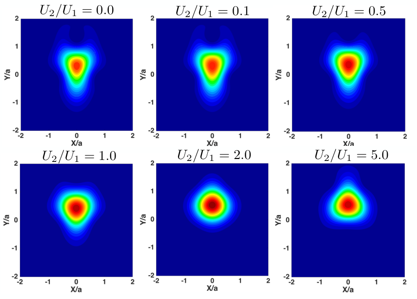
After establishing the dependence of the optimal gauge on the form of interaction, we proceed to see how the optimal gauge evolves with different forms of interactions. We adopt the mixed form of the interaction Eq. (9), and determine optimal gauges for different values of $U_{2}/U_{1}$. Figure 4 shows the evolution of corresponding Wannier functions. We observe that the overall shapes of the Wannier functions undergo clearly visible changes, from a elongated triangle pointing downward for the short-range interaction ($U_{2}/U_{1}=0$), to a nearly equilateral triangle pointing downward when $U_{2}/U_{1}=1$, and to triangles pointing upward when $U_{2}/U_{1}$ is further increased. Actually, the Wannier function for the interaction ($U_{2}/U_{1}\sim 1)$ is very close to that in Wu et al.’s gauge shown in Fig. 2(b).

In Fig. 5, we show the correlation energy corresponding to Qi’s gauge and Wu et al.’s gauge relative to that of the optimal gauge versus the ratio $U_{2}/U_{1}$. We see that the correlation energies of both the gauges can be close to that of the optimal gauge when the strengths of the short-range interaction and the Coulomb interaction are approximately equal ($U_{2}/U_{1}\sim 1$), but deviate significantly when the short-range component of the interaction becomes more prominent ($U_{2}/U_{1}\ll 1$ or $\gg 1$). This is not surprising because our variational degrees of freedom $\theta(\bm{k})$ affects mainly short-range correlations in the trial ground state wave function by modifying the spatial distribution of the Wannier functions. Its effect to a system with a long-range interaction like the Coulomb interaction would be minimal. We also observe that while Wu et al.’s gauge can be very close to the optimal gauge when $U_{2}/U_{1}\approx 1$, it actually becomes worse than Qi’s gauge when $U_{2}/U_{1}\gg 1$ . This is because in the regime, both the gauges are qualitatively different from the optimal gauge, and Qi’s gauge is actually relatively closer to the optimal one, as evident from Fig. 4 and Fig. 2(b, c).

References

- [1] D. C. Tsui, H. L. Stormer and A. C. Gossard, Phys. Rev. Lett. 48, 1559 (1982).
- [2] K. v. Klitzing, G. Dorda and M. Pepper, Phys. Rev. Lett. 45, 494 (1980).
- [3] D. J. Thouless, M. Kohmoto, M. P. Nightingale and M. den Nijs, 49, 405 (1982).
- [4] R. B. Laughlin, Phys. Rev. Lett. 50, 1395 (1983).
- [5] J. K. Jain, Phys. Rev. Lett. 63, 199 (1989).
- [6] J. K. Jain, Composite Fermions (Cambridge University Press, Cambridge, England, 2007).
- [7] F. D. M. Haldane, Phys. Rev. Lett. 51, 605 (1983).
- [8] G. Moore and N. Read, Nucl. Phys. B 360, 362(1991) See also N. Read and G. Moore, Prog. Theor. Phys. Suppl. 107, 157 (1992).
- [9] C. Nayak, S. H. Simon, A. Stern, M. Freedman and S. Das Sarma, Rev. Mod. Phys. 80, 1083 (2008).
- [10] D. N. Sheng, Z. Gu, K. Sun, and L. Sheng, Nature Commun. 2, 389 (2011).
- [11] K. Sun, Z. Gu, H. Katsura, and S. Das Sarma, Phys. Rev. Lett. 106, 236803 (2011).
- [12] T. Neupert, L. Santos, C. Chamon, and C. Mudry, Phys. Rev. Lett. 106, 236804 (2011).
- [13] E. Tang, J.-W. Mei, and X.-G. Wen, Phys. Rev. Lett. 106, 236802 (2011).
- [14] Y.-F.Wang, Z.-C. Gu, C.-D. Gong, and D. N. Sheng, Phys. Rev. Lett. 107, 146803 (2011).
- [15] N. Regnault and B. A. Bernevig, Phys. Rev. X 1, 021014 (2011).
- [16] S. A. Parameswaran, R. Roy and S. L. Sondhi, C. R. Physique 14, 816 (2013).
- [17] E. J. Bergholtz and Z. Liu, Int. J. Mod. Phys. B 27, 1330017 (2013).
- [18] T. Neupert, C. Chamon, T. Iadecola, L. H. Santos and C. Mudry4, Phys. Scr. T164 (2015) 014005 (9pp).
- [19] X. L. Qi, Phys. Rev. Lett, 107,126803 (2011).
- [20] Y. L. Wu, N. Regnault and B. A. Bernevig, Phys. Rev. B 86, 085129 (2012).
- [21] Y. L. Wu, N. Regnault and B. A. Bernevig, Phys. Rev. Lett. 110, 106802 (2013).
- [22] Y. L. Wu, N. Regnault and B. A. Bernevig, Phys. Rev. B 89, 155113 (2014).
- [23] Y. H. Zhang and J. R. Shi, Phys. Rev. B 93, 165129 (2016).
- [24] Z. Liu, E. J. Bergholtz, H. Fan, and A. M. Lauchli, Phys. Rev. Lett. 109, 186805 (2012).
- [25] A. Sterdyniak, C. Repellin, B. Andrei Bernevig, and N. Regnault, Phys. Rev. B 87, 205137 (2013).
- [26] M. Trescher and E. J. Bergholtz, Phys. Rev. B 86, 241111 (2012).
- [27] F. Wang and Y. Ran, Phys. Rev. B 84, 241103 (R) (2011).
- [28] Y.-F. Wang, H. Yao, C.-D. Gong, and D. N. Sheng, Phys. Rev. B 86, 201101 (2012).
- [29] S. Yang, Z. C. Gu, K. Sun and S. Das Sarma, Phys. Rev. B 86, 241112 (2012).
- [30] N. R. Cooper and R. Moessner, Phys. Rev. Lett. 109, 215302 (2012).
- [31] S. M. Girvin, A. H. MacDonald, P. M. Platzman, Phys. Rev. B 33, 2481 (1986).