Self-Similarity Based Time Warping
Abstract
In this work, we explore the problem of aligning two time-ordered point clouds which are spatially transformed and re-parameterized versions of each other. This has a diverse array of applications such as cross modal time series synchronization (e.g. MOCAP to video) and alignment of discretized curves in images. Most other works that address this problem attempt to jointly uncover a spatial alignment and correspondences between the two point clouds, or to derive local invariants to spatial transformations such as curvature before computing correspondences. By contrast, we sidestep spatial alignment completely by using self-similarity matrices (SSMs) as a proxy to the time-ordered point clouds, since self-similarity matrices are blind to isometries and respect global geometry. Our algorithm, dubbed “Isometry Blind Dynamic Time Warping” (IBDTW), is simple and general, and we show that its associated dissimilarity measure lower bounds the L1 Gromov-Hausdorff distance between the two point sets when restricted to warping paths. We also present a local, partial alignment extension of IBDTW based on the Smith Waterman algorithm. This eliminates the need for tedious manual cropping of time series, which is ordinarily necessary for global alignment algorithms to function properly.
1 Introduction / Background

In this work, we address the problem of synchronizing sampled curves, which we refer to as “time-ordered point clouds” (TOPCs). The problem of synchronizing TOPCs which trace similar trajectories but which may be parameterized differently is usually approached with the Dynamic Time Warping (DTW) algorithm [31, 32]. Since sequential data can often be translated into a sequence of vectors in some feature space, this algorithm has found widespread use in applications such as spoken word synchronization [31, 32], gesture recognition [37], touch screen authentication [12], video contour shape sequence alignment [26], and general time series alignment [5], to name a few of the thousands of works that use it. The problem becomes substantially more difficult, however, when the point clouds undergo spatial transformations or dimensionality shifts in addition to re-parameterizations, which is more common across modalities. For instance, one may want to synchronize a motion capture sequence expressed with quaternions of joints with a video of a similar motion in some feature space (see Section 5.4). There is no apparent correspondence between these spaces a priori. This problem even arises within modalities, such as aligning gestures from different people who reside in different spatial locations. Thus, when synchronizing sampled curves, it is important to address not only re-parameterizations, but also spatial transformations such as maps between spaces or rotations/translations/flips within the same space.
In our work, we avoid explicitly solving for spatial maps by using self-similarity matrices (SSMs). Figure 1 shows a sketch of the technique. Even if the curves have been rotated/translated/flipped and re-parameterized, rows of the SSMs which are in correspondence are re-parameterized versions of each other. Our technique is simple both conceptually and in implementation, it is fully unsupervised, and it is parameter free. There are also theoretical connections between our algorithm and metric geometry, as shown in Section 2.2. We also show an extension of our basic technique to partially align time series across modalities (Section 3), and this is the first known solution to that problem. Finally, with proper normalization (Section 4), these techniques can address cross-modal alignment. We show favorable results on a number of benchmark datasets (Section 5).
1.1 Self-Similarity Matrices (SSMs)
The main data structure we rely on in this work is the self-similarity matrix. Given a space curve parameterized by the unit interval , a Self-Similarity Image (SSI) is a function so that
| (1) |
The discretized version of an SSI corresponding to a sampled version of a curve is a self-similarity matrix (SSM). SSIs and SSMs are naturally blind to isometries of the underlying space curve and time-ordered point cloud, respectively; these structures remain the same if the curve/point cloud is rotated/translated/flipped.
Time-ordered SSMs have been applied to the problem of human activity recognition in video [20], periodicity and symmetry detection in video motion [11], musical audio note boundary detection [14], music structure understanding and segmentation [4, 23, 35, 28], cover song identification [39], and dynamical systems [29], to name a few areas. In this work, we study more general properties of time-ordered SSMs that make them useful for alignment.
1.2 Warping Paths / Dynamic Time Warping
The warping path is the basic primitive object we seek to synchronize two time-ordered point clouds. It is a discrete version of an orientation preserving homeomorphism of the unit interval used to re-parameterize curves. In layman’s terms, it provides a way to step forward along both point clouds jointly in a continuous way without backtracking, so that they are optimally aligned over all steps. More precisely, given two sets and , a correspondence between the two sets is such that and s.t. and s.t. . In other words, a correspondence is a matching between two sets and so that each element in is matched to at least one element in , and each element of is matched to at least one element in . Let and be two sets whose elements are adorned with a time order: and . A warping path, between and is a correspondence which can be put into the sequence satisfying the following properties
- •
Monotonicity: If , then for ,
- •
Boundary Conditions:
- •
Continuity:
Now suppose there are two time-ordered point clouds and which both live in the same metric space . The Dynamic Time Warping (DTW) Dissimilarity[31, 32]11 1 Note that DTW is not a metric, as it fails to satisfy the triangle inequality. For an example, see [30] section 4.1 between and is
where is the set of all valid warping paths between and . DTW satisfies the following subsequence relation
| (2) |
where is the DTW dissimilarity between and . This makes it possible to solve DTW with a dynamic programming algorithm which takes time. This algorithm computes the cost of the shortest path from the upper left to the lower right of the “cross-similarity matrix” (CSM), or the matrix holding all distances between and . A (not necessarily unique) shortest path realizing this distance is a warping path which can be used to align the two time series.
1.3 DTW After Spatial Transformations
In addition to synchronizing curves in the same ambient space which are approximately re-parameterizations of each other, there has also been some recent work on the more difficult problem of matching curves which live in different ambient spaces or which live in the same space but which may differ by a spatial transformation in addition to re-parameterization. One objective for spatial alignment is the optimal rigid transformation taking one set of points to another. More precisely, given two Euclidean point clouds , each with points which are assumed to be in correspondence, the Procrustes distance [46, 22] is
| (3) |
One issue with Procrustes is that not only do and have to have the same number of points, but the correspondences must be known a priori. Often in practice, neither of these assumptions are true. To deal with this, one can use the “Iterative Closest Points” (ICP) algorithm [6, 8], which switches back and forth between finding correspondences with nearest neighbors and solving the Procrustes problem. The authors of [49] use a modified version of ICP, replacing the nearest neighbor correspondence step with DTW. This ensures that the time order will be respected, which is not guaranteed with nearest neighbors only22 2 This analogous to the difference between the Fréchet Distance [2] and the Hausdorff Distance between curves..
There are also techniques which use canonical correlation analysis (CCA) instead of Procrustes analysis. Given two point clouds with points represented by matrices and , assumed to be in correspondence, CCA is defined as
| (4) |
for some chosen constant , s.t. . This is better suited to cross modal applications where scaling is involved. Like Procrustes, this assumes that the correspondences are known a priori. To find the correspondences, the authors in [53] take the same iterative approach as that authors in [49] did with ICP, but they alternate back and forth between DTW and CCA instead of DTW and Procrustes. An updated version of this algorithm known as “generalized time warping” (GTW) [51, 52] was developed which aligns multiple sequences using a single optimization objective where the spatial alignment and time warping are coupled. Finally, a recent work in [40, 41] takes a similar approach, but it replaces CCA by learning features in the projection stage with a deep neural network. Like all supervised learning approaches, however, this method requires training data with known correspondences. Furthermore, all of the techniques we have mentioned so far require a good initial guess to converge to a globally optimal solution.
As an alternative to solving for a spatial alignment explicitly, many works perform time warping on a surrogate function which is invariant to isometries of the input. A popular choice is to numerically estimate curvature [24, 33, 15]. Some works use the triangle area between triples of points as an invariant [1], and some use the turning angle of the curve [9], which is related to curvature. These techniques can suffer from numerical difficulties when estimating the invariants. Also, most of the invariants are local, so small differences can cause the curves “drift” over time (e.g. a U is similar to a 6 with local curvature [33]), though using integrated curvature [10] can ameliorate this.
Beyond spatial alignment and invariants, the authors of [47] address more general case of cross-domain object matching (CDOM) with general correspondences and address warping paths as a special case. However, their problem reduces to the quadratic assignment problem, which is NP-hard, and their iterative approximation requires a good initial guess. The authors of [42] address a special case where curves form closed loops, using cohomology to find maps from point clouds to the circle, where they are synchronized, but this only works for periodic time series. The authors of [16] jointly align curves on manifolds, which is effective but requires learning the manifolds. Perhaps the most similar to our approach is the action recognition work of [21], from which we drew much inspiration, which applies DTW to small patches of SSMs to align time warped actions from different camera views. However, they only use elements near the diagonal of SSMs, and their scheme does not extend across modalities.
2 Isometry Blind Dynamic Time Warping

Most of the approaches we reviewed to align time series which have undergone linear transformations try to explicitly factor out those transformations before doing an alignment, but this is not necessary if we build our algorithm on top a self-similarity matrix between two point clouds, which is already blind to isometries. To set the stage for our algorithms, we first study the maps that are induced between self-similarity images by re-parameterization functions, which will help in the algorithm design. For example, take the figure 8 curve,. The bottom left of Figure 2 shows the SSM of a linearly parameterized sampled version of this curve, while the bottom right of Figure 2 shows the SSM corresponding to a re-parameterized sampled version. Maps between the domains of the SSMs shown are always rectangles, and they are independent of underlying curve being parameterized (they only depend on the relationship between two parameterizations). To see this, start with a space curve and its resulting self-similarity image . Given a homeomorphism , which yields a space curve and a corresponding self-similarity image , there is an induced homeomorphism, from the square to itself between the two domains of and ; that is, . If we fix a correspondence , then this shows that row of is a 1D re-parameterization of row of , making rigorous the observation in Figure 1. Note that for a discrete version of these maps between time-ordered point clouds, one can replace the homeomorphism with a warping path , and the relationships are otherwise the same.
2.1 IBDTW Algorithm
We now have the prerequisites necessary to define our main algorithm. The idea is quite simple. Based on our observations and Figure 1 and Figure 2, if we know that point in a time-ordered point cloud (TOPC) is in correspondence with a point in TOPC Y, then we should match the row of X’s SSM to the row of Y’s SSM under the distance, enforcing the constraint that . However, since it is unknown a priori which rows should be in correspondence, we try every row of SSM A against every row in SSM B, and we create a cross-similarity time warping matrix (CSWM) so that contains DTW between row of SSMA and row of SSMB, constrained to warping paths which include . To enforce that be in the optimal warping path, we exploit the boundary condition property of DTW by running the original DTW algorithm twice: once between and once between and , summing the costs. After doing this , apply the ordinary DTW algorithm to . Algorithm 1 summarizes this process. Note that a serial implementation of this algorithm takes time, since a 1D DTW is computed for every row pair. To mitigate this, we implement a linear systolic array[50] version of DTW in CUDA. With unlimited parallel processors, this reduces computation to . In practice, we witness a 30x speedup between point clouds with hundreds of samples.
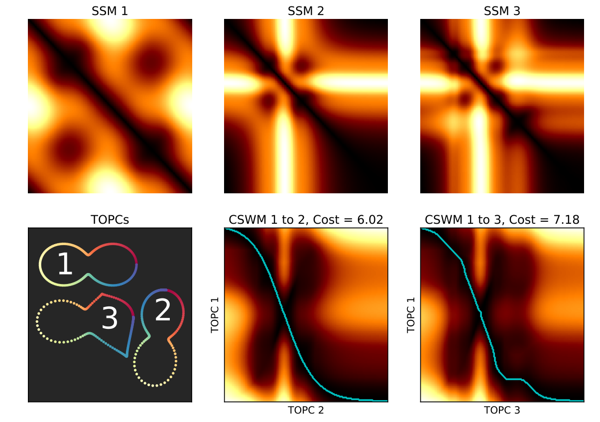
Figure 3 shows an example of this algorithm on two rotated/translated/re-parameterized time-ordered point clouds in (point clouds 1 and 2). As the colors show, IBDTW puts the points into correspondence correctly even without first spatially aligning them. We also show alignment to a third time-ordered point cloud, which is metrically distorted in addition to being rotated/translated/re-parameterized. The returned warping degrades gracefully. We will explore this more rigorously in Section 5.1.
2.2 Analysis: Lower Bounding L1 Metric Stress
IBDTW can be put into the Gromov-Hausdorff Distance framework, which describes how to “embed” one metric space into another. More formally, given two discrete metric spaces and , and a correspondence between and , the -stress is defined as
| (5) |
Intuitively, the -stress measures how much one has to stretch one metric space when moving it to another. The Gromov-Hausdorff Distance uses specifically:
| (6) |
where is the set of all correspondences between and . In other words, the Gromov-Hausdorff Distance measures the smallest possible distortion between a pair of points over all possible embeddings of one metric space into another. Unfortunately, the Gromov-Hausdorff Distance is NP-complete, but we can still connect Algorithm 1 to the Gromov-Hausdorff Distance via the following lemma:
Lemma 1.
The cost returned by Algorithm 1 lower bounds , or the 1-stress restricted to warping paths.
Proof: Note that the optimal IBDTW warping path has the following cost
| (7) |
which can be rewritten as
| (8) |
since if then the cost is zero, all other terms counted twice. Now fix an and . Then the sum of the terms of the form is simply the warping distance between 1D time series which are the row of , and the row of , under the warping . Also, the DTW Distance between and is at most the warping distance under , and is potentially lower since we are computing them greedily only between and , ignoring all other constraints. Hence, the sum of the terms is lower bounded by Line 11 in Algorithm 1.
For a more direct analogy with DTW, Algorithm 1 was designed to lower bound the 1-stress restricted to warping paths. We note that a similar technique could be used to lower bound the Gromov-Hausdorff Distance restricted to warping paths by replacing constrained DTW in the inner loop in Line 11 with a constrained version of the discrete Fréchet Distance [13] to find the maximum distortion induced by putting two points in correspondence. In this work, however, we stick to the 1-stress, since it gives a more informative overall picture of the full metric space.
3 Isometry Blind Partial Time Warping
One of the drawbacks of IBDTW is that it requires a global alignment. However, if the sequences only partially overlap, forcing a global alignment leads to poor result, unless manual cropping is done to ensure that sequences start and end at the same place [53]. To automate cropping, we design an isometry blind time warping algorithm that can do partial alignment. This algorithm is like IBDTW, except DTW is replaced with the “Smith Waterman” algorithm [36, 45], which seeks the best contiguous subsequences in each time series which match each other 33 3 This algorithm was originally developed for gene sequence alignment, but it has been adapted to multimedia problems such as music alignment [34] and video copyright infringement detection [7].. Unlike dynamic time warping, Smith Waterman seeks to maximize an alignment score, and the alignment does not have to start on the first element of each sequence or end on the last element on each sequence. To solve this, the exact same dynamic programming algorithm is used, except there is one extra “restart” condition if a local alignment has become sufficiently poor. The recurrence is
| (9) |
where is a matching score between points and , which is positive for a match and negative for a mismatch, and is a gap penalty.

Like DTW, we may modify Smith Waterman to return the best subsequence constrained to match the point in the first sequence to the point in the second sequence by runing Smith Waterman between and , and then again between the reversed sequences and . Then, the Isometry Blind Partial Time Warping (IBPTW) algorithm is exactly like Algorithm 1, except we replace Line 11 with constrained Smith Waterman, and we replace Line 15 with unconstrained Smith Waterman. We refer to the matrix (Line 4) as the “partial cross-similarity warp matrix (PCSWM).” In practice, we define for Line 11. If is the L1 distance between elements of two histogram normalized SSM rows, then it ranges between and . Thus, there is a positive matching score of up to 0.4 for the most similar SSM values and a negative matching score of -0.6 between the most dissimilar values. We also choose a gap penalty of -0.4 to promote diagonal matches. Otherwise, the warping path maximizing the alignment score contains longer horizontal and vertical lines, leading to undesirable pauses of one time series with respect to the other. For the outer loop (Line 15), we use
where md is the median operation. This will give a high score up to to row pairs which have a high subsequence score in common, and a low score to rows which do not have a good subsequence. Figure 4 shows an example of this algorithm on two jigsaw puzzle pieces which should fit together with and defined as above, , and . The longest subsequence is indeed along the cutouts where they match together. It is also possible to backtrace from anywhere in the PCSWM to find other subsequences which match in common, so Figure 4 also shows an example of suboptimal but good local alignment.
4 Cross-Modal Histogram Normalization

The schemes we have presented work well for point clouds sampled from isometric curves, but the isometry assumption does not usually hold in cross-modal applications. Not only can the scales be drastically different between modalities, but it is unlikely that a uniform re-scaling will fix the problem. For instance, consider a 1D oscillating bar of length oscillating sinusoidally over the interval with a period of . Its center position is measured as . This type of measurement, which follows the object in question, is in Lagrangian coordinates. By contrast, suppose we take a 1D video of the bar with pixels, where each pixel in each frame measures occupancy by the bar at that frame in the video. Then pixel in video is parameterized by time as
| (10) |
These pixel by pixel measurements at fixed positions are referred to as Eulerian coordinates. Let the Lagrangian SSM be the 1D metric between two different centers, , and let the Eulerian SSM be the Euclidean metric between each frame of the video. Although they are measuring the same process, the SSMs have a locally different character. Rows of are perfect sinusoids, while rows of are more like square waves, since there are sharp transitions from foreground to background in Eulerian coordinates. Figure 5 summarizes all of this visually.
To address this kind of local rescaling between an SSM and an SSM , we first divide each SSM by its respective max, and we quantize each to levels evenly spaced in . We then apply a monotonic, one-to-one map to each pixel in so that the CDF of approximately matches the CDF of (see, e.g., [17] ch. 3.3). Note that this process can be done from to or from to , as shown in Figure 5. Since this process is not necessarily symmetric, we perform both sets of normalizations, and we choose the one which yields a better alignment score.
5 Experimental Results
In this section, we will quantitatively compare the IBDTW algorithm for global alignment with several other techniques in the literature, including ordinary dynamic time warping (DTW), derivative dynamic time warping (DDTW) [24] (a curvature-based version), canonical time warping (CTW)[53], Generalized Time Warping (GTW)[51, 52], and Iterative Motion Warping (IMW)[19] (a simpler version of CTW which is restricted to the same space). We use code from [53] and [51, 52] to compute all of these alignments44 4 http://www.f-zhou.com/ta_code.html. We use the default parameters provided in this code, and, as in [53] and [51, 52], we use the results of DTW to initialize CTW and GTW. In all of our experiments, we show results both from IBDTW and IBDTW after SSM rank normalization, which we refer to as “IBDTWN.” When a ground truth warping path exists, we report the alignment error as in [52] and [40]. Given a warping path and a ground truth path , the alignment error is
| (11) |
which is (roughly) the average number of samples by which is shifted from at any point in time.
5.1 Curve Alignment

We first perform an experiment aligning a series of rotated/translated/flipped and re-parameterized sampled curves. As in [52], we re-parameterize the curves with random convex combinations of polynomial, logarithmic, exponential, and hyperbolic tangent functions. To distort the curves, we move random control points in random directions after spatial transformation and re-parameterization. Let be the TOPC before transformation/re-paramterization/distortion and let be the curve afterwards. The average ratio of , where diam is the “diameter” of (the maximum inter point distance), is 0.18. Figure 6 shows the results. IBDTW performs the best, while doing the normalization for IBDTWN only degrades the results slightly.
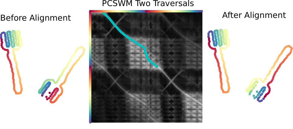
We also showcase our IBPTW algorithm by aligning 2D loops, or curves so that , which is useful in recognizing boundaries of foreground objects in video. Note that a geometrically equivalent loop can be parameterized starting at a different point in the interior of the first loop: . Also, it is possible that this loop is parameterized differently: for some orientation preserving homeomorphism , and may also be transformed spatially. To demonstrate how our algorithm is able to align such curves, we use examples from the MPEG-7 dataset of 2D contours [25]. Given a point cloud and a point cloud , we partially align the concatenated point clouds and . If starts samples later than , then there will be a partial warping path which starts at sample in and sample in . Figure 7 shows an example where two forks are successfully put into correspondence this way. Figure 8 shows a histogram of alignment errors for distorted/circularly shifted/re-parameterized curves over 7 classes from the MPEG-7 dataset, using and , and with a mean . IBPTW returns excellent alignments for most loops, though there are a cluster of outliers that occur due to (near) symmetries of some loops.
5.2 Weizmann Walking Videos
For our first cross modal experiment, we align 4 videos of people walking from the Weizmann dataset [18] cropped to 4 walking cycles each. As in [53], we use different features between each pair of videos we align. On one video, we use the binary mask of the foreground object of the person walking, where every pixel is a dimension, and every frame is a point in the TOPC. On the second video, we use the Euclidean distance transform (EDT) [27]. To assess performance rigorously, we create a more controlled experiment where the second video is the same as the first video after a time warp and applying EDT, so that we have access to the ground truth. Figure 9 shows the results. CTW performs slightly better than IBDTWN, but not appreciably. Furthermore, IBTW without normalization has the worst average alignment error, demonstrating how normalization is needed in cross-modal applications.
5.3 BU4D 2D/3D Facial Expressions
To show a more difficult cross-modal application, we also synchronize expressions drawn from the BU4D face dataset [48], which includes RGB videos of people making different facial expressions and a 3D triangle mesh corresponding to each frame. For our RGB features, we simply take each channel and each pixel to be a dimension, so a video with pixels lives in . For the 3D mesh features, we use shape histograms [3] after mean centering and RMS normalizing each mesh. Our shape histograms have 20 radial shells, each with 66 sectors per shell with centers equally distributed across the sphere. We perform an experiment where we take the 2D features from a face and the 3D features of the same face which has been warped in time. We perform 10 such warpings and alignments for 9 faces from 6 different expression types. Figure 9 shows the aggregated results. The performance is strikingly worse than the Weizmann dataset, though the normalized IBDTW has about half of the alignment error of other techniques.
5.4 Non-Euclidean Examples


One strength of our algorithms is that they run without modification for features in arbitrary metric spaces. For example, Figure 10 shows IBDTW between motion capture data expressed in a product space of quaternions of joints with video data expressed as raw pixels. The product space of quaternions we choose is between two sets of quaternions and . For our second example, Figure 11 shows IBPTW used to align two “cover songs” (two versions of the same song with different instruments / tempos) after fusing note-based and timbral features using similarity network fusion [43, 44] to learn an improved metric for self-similarity (see [38] for more info on this process). Please also refer to supplementary material for video and audio for these examples.
6 Conclusions
In this work, we have shown it is possible to synchronize time-ordered point clouds that are spatially transformed without explicitly uncovering the spatial transformation. As we have shown by our experiments, our algorithms perform excellently when aligning nearly isometric sampled curves, and, with proper normalization, we are competitive with state of the art unsupervised techniques for cross-modal applications. Furthermore, IBDTW requires no parameters, making it approachable “out of the box,” while, in our experience, CTW and GTW require many parameters that make or break performance. Finally, we have opened the door for straightforward non-Euclidean time warping, and we hope to see more such applications (e.g. time series of graphs).
Acknowledgments
Christopher Tralie was partially supported by an NSF Graduate Fellowship NSF under grant DGF-1106401 and an NSF big data grant DKA-1447491. Paul Bendich is thanked for the suggestion to compare the technique to the Gromov-Hausdorff Distance, and for helpful comments on an initial manuscript.
References
- [1] N. Alajlan, I. El Rube, M. S. Kamel, and G. Freeman. Shape retrieval using triangle-area representation and dynamic space warping. Pattern Recognition, 40(7):1911–1920, 2007.
- [2] H. Alt and M. Godau. Computing the fréchet distance between two polygonal curves. International Journal of Computational Geometry & Applications, 5(01n02):75–91, 1995.
- [3] M. Ankerst, G. Kastenmüller, H.-P. Kriegel, and T. Seidl. 3d shape histograms for similarity search and classification in spatial databases. In International Symposium on Spatial Databases, pages 207–226. Springer, 1999.
- [4] J. P. Bello. Grouping recorded music by structural similarity. Int. Conf. Music Inf. Retrieval (ISMIR-09), 2009.
- [5] D. J. Berndt and J. Clifford. Using dynamic time warping to find patterns in time series. In KDD workshop, volume 10, pages 359–370. Seattle, WA, 1994.
- [6] P. J. Besl and N. D. McKay. Method for registration of 3-d shapes. In Robotics-DL tentative, pages 586–606. International Society for Optics and Photonics, 1992.
- [7] A. M. Bronstein, M. M. Bronstein, and R. Kimmel. The video genome. arXiv preprint arXiv:1003.5320, 2010.
- [8] Y. Chen and G. Medioni. Object modelling by registration of multiple range images. Image and vision computing, 10(3):145–155, 1992.
- [9] S. D. Cohen and L. J. Guibas. Partial matching of planar polylines under similarity transformations. In SODA, pages 777–786, 1997.
- [10] M. Cui, J. Femiani, J. Hu, P. Wonka, and A. Razdan. Curve matching for open 2d curves. Pattern Recognition Letters, 30(1):1–10, 2009.
- [11] R. Cutler and L. S. Davis. Robust real-time periodic motion detection, analysis, and applications. IEEE Transactions on Pattern Analysis and Machine Intelligence, 22(8):781–796, 2000.
- [12] A. De Luca, A. Hang, F. Brudy, C. Lindner, and H. Hussmann. Touch me once and i know it’s you!: implicit authentication based on touch screen patterns. In Proceedings of the SIGCHI Conference on Human Factors in Computing Systems, pages 987–996. ACM, 2012.
- [13] T. Eiter and H. Mannila. Computing discrete fréchet distance. Technical report, Citeseer, 1994.
- [14] J. Foote. Automatic audio segmentation using a measure of audio novelty. In Multimedia and Expo, 2000. ICME 2000. 2000 IEEE International Conference on, volume 1, pages 452–455. IEEE, 2000.
- [15] M. Frenkel and R. Basri. Curve matching using the fast marching method. In EMMCVPR, pages 35–51. Springer, 2003.
- [16] D. Gong and G. Medioni. Dynamic manifold warping for view invariant action recognition. In Computer Vision (ICCV), 2011 IEEE International Conference on, pages 571–578. IEEE, 2011.
- [17] R. Gonzalez and R. Woods. Digital Image Processing. Addison-Wesley world student series. Addison-Wesley, 1992.
- [18] L. Gorelick, M. Blank, E. Shechtman, M. Irani, and R. Basri. Actions as space-time shapes. Transactions on Pattern Analysis and Machine Intelligence, 29(12):2247–2253, December 2007.
- [19] E. Hsu, K. Pulli, and J. Popović. Style translation for human motion. In ACM Transactions on Graphics (TOG), volume 24, pages 1082–1089. ACM, 2005.
- [20] I. N. Junejo, E. Dexter, I. Laptev, and P. Pérez. Cross-view action recognition from temporal self-similarities. In Proceedings of the 10th European Conference on Computer Vision: Part II, pages 293–306. Springer-Verlag, 2008.
- [21] I. N. Junejo, E. Dexter, I. Laptev, and P. Perez. View-independent action recognition from temporal self-similarities. IEEE transactions on pattern analysis and machine intelligence, 33(1):172–185, 2011.
- [22] W. Kabsch. A solution for the best rotation to relate two sets of vectors. Acta Crystallographica Section A: Crystal Physics, Diffraction, Theoretical and General Crystallography, 32(5):922–923, 1976.
- [23] F. Kaiser and T. Sikora. Music structure discovery in popular music using non-negative matrix factorization. In ISMIR, pages 429–434, 2010.
- [24] E. J. Keogh and M. J. Pazzani. Derivative dynamic time warping. In Proceedings of the 2001 SIAM International Conference on Data Mining, pages 1–11. SIAM, 2001.
- [25] L. Latecki. Shape data for the mpeg-7 core experiment ce-shape-1. Web Page: http://www. cis. temple. edu/˜ latecki/TestData/mpeg7shapeB. tar. g z, 2002.
- [26] P. Maurel and G. Sapiro. Dynamic shapes average. 2003.
- [27] C. R. Maurer, R. Qi, and V. Raghavan. A linear time algorithm for computing exact euclidean distance transforms of binary images in arbitrary dimensions. IEEE Transactions on Pattern Analysis and Machine Intelligence, 25(2):265–270, 2003.
- [28] B. McFee and D. P. Ellis. Analyzing song structure with spectral clustering. In 15th International Society for Music Information Retrieval (ISMIR) Conference, 2014.
- [29] G. McGuire, N. B. Azar, and M. Shelhamer. Recurrence matrices and the preservation of dynamical properties. Physics Letters A, 237(1-2):43–47, 1997.
- [30] M. Müller. Information retrieval for music and motion, volume 2. Springer, 2007.
- [31] H. Sakoe and S. Chiba. A similarity evaluation of speech patterns by dynamic programming. In Nat. Meeting of Institute of Electronic Communications Engineers of Japan, page 136, 1970.
- [32] H. Sakoe and S. Chiba. Dynamic programming algorithm optimization for spoken word recognition. IEEE transactions on acoustics, speech, and signal processing, 26(1):43–49, 1978.
- [33] T. B. Sebastian, P. N. Klein, and B. B. Kimia. On aligning curves. IEEE transactions on pattern analysis and machine intelligence, 25(1):116–125, 2003.
- [34] J. Serra, E. Gómez, P. Herrera, and X. Serra. Chroma binary similarity and local alignment applied to cover song identification. Audio, Speech, and Language Processing, IEEE Transactions on, 16(6):1138–1151, 2008.
- [35] J. Serra, M. Müller, P. Grosche, and J. L. Arcos. Unsupervised detection of music boundaries by time series structure features. In Twenty-Sixth AAAI Conference on Artificial Intelligence, 2012.
- [36] T. F. Smith and M. S. Waterman. Identification of common molecular subsequences. Journal of molecular biology, 147(1):195–197, 1981.
- [37] G. A. ten Holt, M. J. Reinders, and E. Hendriks. Multi-dimensional dynamic time warping for gesture recognition. In Thirteenth annual conference of the Advanced School for Computing and Imaging, volume 300, 2007.
- [38] C. J. Tralie. Early mfcc and hpcp fusion for robust cover song identification. In 18th International Society for Music Information Retrieval (ISMIR), 2017.
- [39] C. J. Tralie and P. Bendich. Cover song identification with timbral shape. In 16th International Society for Music Information Retrieval (ISMIR) Conference, 2015.
- [40] G. Trigeorgis, M. Nicolaou, S. Zafeiriou, and B. Schuller. Deep canonical time warping for simultaneous alignment and representation learning of sequences. IEEE Transactions on Pattern Analysis and Machine Intelligence, 2017.
- [41] G. Trigeorgis, M. A. Nicolaou, S. Zafeiriou, and B. W. Schuller. Deep canonical time warping. In Proceedings of the IEEE Conference on Computer Vision and Pattern Recognition, pages 5110–5118, 2016.
- [42] M. Vejdemo-Johansson, F. T. Pokorny, P. Skraba, and D. Kragic. Cohomological learning of periodic motion. Applicable Algebra in Engineering, Communication and Computing, 26(1-2):5–26, 2015.
- [43] B. Wang, J. Jiang, W. Wang, Z.-H. Zhou, and Z. Tu. Unsupervised metric fusion by cross diffusion. In Computer Vision and Pattern Recognition (CVPR), 2012 IEEE Conference on, pages 2997–3004. IEEE, 2012.
- [44] B. Wang, A. M. Mezlini, F. Demir, M. Fiume, Z. Tu, M. Brudno, B. Haibe-Kains, and A. Goldenberg. Similarity network fusion for aggregating data types on a genomic scale. Nature methods, 11(3):333–337, 2014.
- [45] M. S. Waterman. Introduction to computational biology: maps, sequences and genomes. CRC Press, 1995.
- [46] G. Whaba. A least squares estimate of spacecraft attitude. SIAM Review, 7(3):409, 1965.
- [47] M. Yamada, L. Sigal, M. Raptis, M. Toyoda, Y. Chang, and M. Sugiyama. Cross-domain matching with squared-loss mutual information. IEEE transactions on pattern analysis and machine intelligence, 37(9):1764–1776, 2015.
- [48] L. Yin, X. Chen, Y. Sun, T. Worm, and M. Reale. A high-resolution 3d dynamic facial expression database. In Automatic Face & Gesture Recognition, 2008. FG’08. 8th IEEE International Conference on, pages 1–6. IEEE, 2008.
- [49] R. Ying, J. Pan, K. Fox, and P. K. Agarwal. A simple efficient approximation algorithm for dynamic time warping. In Proceedings of the 24th ACM SIGSPATIAL International Conference on Advances in Geographic Information Systems, GIS ’16, pages 21:1–21:10, New York, NY, USA, 2016. ACM.
- [50] C. W. Yu, K. Kwong, K.-H. Lee, and P. H. W. Leong. A smith-waterman systolic cell. In New Algorithms, Architectures and Applications for Reconfigurable Computing, pages 291–300. Springer, 2005.
- [51] F. Zhou and F. De la Torre. Generalized time warping for multi-modal alignment of human motion. In Computer Vision and Pattern Recognition (CVPR), 2012 IEEE Conference on, pages 1282–1289. IEEE, 2012.
- [52] F. Zhou and F. De la Torre. Generalized canonical time warping. IEEE transactions on pattern analysis and machine intelligence, 38(2):279–294, 2016.
- [53] F. Zhou and F. Torre. Canonical time warping for alignment of human behavior. In Advances in neural information processing systems, pages 2286–2294, 2009.